message exchange mechanisms and processing techniques

IEEE SIGNAL PROCESSING MAGAZINE [124] JANUARY 2011 1053-5888/11/$26.00©2011IEEE

[Yik-Chung Wu, Qasim Chaudhari,

and Erchin Serpedin]

[Message exchange

mechanisms and

statistical signal

processing techniques]

Clock synchronization is a critical component in theoperation of wireless sensor networks (WSNs), as itprovides a common time frame to different nodes. Itsupports functions such as fusing voice and video datafrom different sensor nodes, time-based channel shar-

ing, and coordinated sleep wake-up node scheduling mechanisms. Earlystudies on clock synchronization for WSNs mainly focused on protocoldesign. However, the clock synchronization problem is inherently relatedto parameter estimation, and, recently, studies on clock synchronizationbegan to emerge by adopting a statistical signal processing framework. Inthis article, a survey on the latest advances in the field of clock synchroniza-tion of WSNs is provided by following a signal processing viewpoint. This arti-cle illustrates that many of the proposed clock synchronization protocols canbe interpreted and their performance assessed using common statistical signalprocessing methods. It is also shown that advanced signal processing techniquesenable the derivation of optimal clock synchronization algorithms under chal-lenging scenarios.

Digital Object Identifier 10.1109/MSP.2010.938757Date of publication: 17 December 2010

© DIGITAL VISION & JOHN FOXX

IEEE SIGNAL PROCESSING MAGAZINE [125] JANUARY 2011

INTRODUCTIONWith the help of recent tech-nological advances in micro-electromechanical systems andwireless communications, low-cost, low-power, and multi-functional wireless sensingdevices have been developed.When these devices are deployed over a wide geographicalregion, they can collect information about the environment andefficiently collaborate to process such information, forming theso-called WSNs. WSNs are a special case of wireless ad hoc net-work and assume a multihop communication without a com-mon infrastructure, where the sensors spontaneously cooperateto deliver information by forwarding packets from a source to adestination. The feasibility of WSNs keeps growing rapidly, andWSNs have been regarded as fundamental infrastructures forfuture ubiquitous communications due to a variety of promisingpotential applications: monitoring the health status of humans,animals, plants, and the environment; control and instrumenta-tion of industrial machines and home appliances; homelandsecurity; and detection of chemical and biological threats [1], [2].

Clock synchronization is a procedure for providing a commonnotion of time across a distributed system. It is crucial for WSNsin performing a number of fundamental operations:

n Data Fusion: Data fusion is a basic operation in all dis-tributed networks for processing and integrating the col-lected data in a meaningful way. It requires some or allnodes in the network to share a common time scale.n Power Management: Energy efficiency is a key design-ing factor for WSNs since sensors are usually left unat-tended without any maintenance and battery replacementservice along their lifetimes. Most energy-saving opera-tions strongly depend on time synchronization. For in-stance, the duty cycling (sleep and wake-up modescontrol) helps the nodes to save huge energy resources byspending minimal power during the sleep mode. There-fore, network-wide synchronization is essential for effi-cient duty cycling, and its performance is proportional tothe synchronization accuracy.n Transmission Scheduling: Many scheduling protocolsrequire clock synchronization. For example, the time divi-sion multiple access scheme, one of the most popular com-munications schemes for distributed networks, is onlyapplicable in a synchronized network.Moreover, many localization, security, and tracking proto-

cols also demand the sensor nodes to timestamp their messagesand sensing events. Therefore, clock synchronization appears asone of the most important research challenges in the design ofenergy-efficient WSNs.

DEFINITION OF CLOCKEvery individual sensor in a network has its own clock. Ideally,the clock of a sensor node should be configured such thatC(t) ¼ t, where t stands for the ideal or reference time. However,

because of the imperfections ofthe clock oscillator, a clock willdrift away from the ideal timeeven if it is initially perfectlytuned. For example, accordingto the data sheet of a typicalcrystal-quartz oscillator com-monly used in sensor net-

works, the frequency of a clock varies up to 40 ppm, whichmeans clocks of different nodes can loose as much as 40 ls in asecond (or 0.144 s in an hour). In general, the clock function ofthe ith node is modeled as

Ci(t) ¼ hþ f � t, (1)

where the parameters h and f are called clock offset (phase differ-ence) and clock skew (frequency difference), respectively. Agraphical representation of the clock model is illustrated inFigure 1.

From (1), the clock relationship between two nodes, Node Aand Node B, can be represented by

CB(t) ¼ hAB þ f AB � CA(t),

where hAB and f AB stand for the relative clock offset and skewbetween Node A and Node B, respectively. Obviously, if twoclocks are perfectly synchronized, hAB ¼ 0 and f AB ¼ 1. Other-wise, suppose Node A is the reference node, the task of clocksynchronization is to estimate hAB and f AB such that Node B canadjust its own clock or translate its timing information to the timescale of Node Awhen it is necessary. If there are L nodes in the net-work, then the global network-wide synchronization requiresCi(t) ¼ Cj(t) for all i, j ¼ 1, � � � , L, or all the relative clock offsetsand skews are estimated with respect to a reference node.

In the long term, clock parameters are subject to changes dueto environmental or other external effects such as temperature,atmospheric pressure, voltage changes, and hardware aging [3].Hence, in general, the relative clock offset keeps changing with

Real Time

Local C

lock T

ime

Ideal Clock

Slope = f

θ

Slope = 1

Node B Clock

Node A Clock

[FIG1] Clock model of sensor nodes.

DATA FUSION IS A BASIC OPERATIONIN ALL DISTRIBUTED NETWORKS

FOR PROCESSING AND INTEGRATINGTHE COLLECTED DATA IN A

MEANINGFULWAY.


time, which means that the network has to perform periodicclock resynchronization to adjust the clock parameters.

THE CHALLENGEAssumeNodeB needs to be synchronized to Node A. Node A sendsits current time to Node B. If there is absolutely no delay in themessage delivery, Node B can immediately know the differencebetween its clock and that of Node A. Unfortunately, in a real wire-less network, various delays affect the message delivery, makingclock synchronization muchmore difficult than it seems to be. Ingeneral, a series of timing message transmissions is required toestimate the relative clock skews and offsets among nodes. Insome sense, clock synchronization in WSNs can be regarded asthe process of removing the effects of random delays from thetimingmessage transmissions sent across wireless channels.

The various delays present in a message delivery include thefollowing components [4], [5]:

n Send Time: The time spent in building the message atthe application layer, including delays introduced by theoperating system when processing the send request.n Access Time: The waiting time for accessing the channelafter reaching the medium access control (MAC) layer.This is the most significant component and highly variabledepending on the specific MAC protocol.n Transmission Time: The time for transmitting a mes-sage at the physical (PHY) layer.n Propagation Time: The actual time for a message to be trans-mitted from the sender to the receiver in a wireless channel.n Reception Time: The time required for receiving a mes-sage at the PHY layer, which is the same as the transmis-sion time.n Receive Time: Time to construct and send the receivedmessage to the application layer at the receiver.The delay components can also be categorized into two

classes: deterministic (fixed portion) and stochastic (variableportion). The variable portion of delays depends on various net-work parameters (e.g., network status and traffic); therefore, nosingle delay model can be found to fit for every case. Probabilitydensity function (pdf) models that have been proposed for mod-eling random delays in wireless networks include Gaussian,exponential, Gamma, Weibull, and log-normal [6]–[8]. In thefirst half of this article, we focus on Gaussian and exponentialdelay models to illustrate the signal processing aspects in clocksynchronization. The Gaussian model is justified if the delaysare thought to be the addition of numerous independent ran-dom processes due to the central limit theorem. This is sup-ported by [9], where the chi-square test showed that the variableportion of delays can be modeled as Gaussian distributed ran-dom variables (RVs) with 99.8% confidence. On the other hand,a single-server M/M/1 queue can fittingly represent the cumula-tive link delay for point-to-point hypothetical reference connec-tions, where the random delays are independently modeled asexponential RVs [10]. The exponential delay model is also sup-ported by experimental measurements [11], [12]. Toward theend of this article, the assumption on the distribution assumed

by the network delays will be relaxed. Arbitrary network delaydistributions will be assumed and the emphasis will be puttoward developing clock offset estimation techniques that arerobust to the distribution of network delays.

Another challenge that clock synchronization in WSNs facesis the limited and generally nonrechargeable power resources.Clock synchronization is one of the critical components contrib-uting to energy consumption due to the highly energy consum-ing radio transmissions for delivering timing information.Pottie and Kaiser showed in [13] that the radio frequency energyrequired to transmit 1 kb more than 100 m (i.e., 3 J) is equiva-lent to the energy required to execute 3 million instructions.Therefore, developing efficient synchronization algorithms rep-resents an ideal mechanism for trading computational energyfor reduced communication overhead.

REMARK 1If the time stamping occurs at the interface between the MAC- andPHY-layer, among the many sources of message delivery delay, thesend, access, and receive times can be eliminated [5]. This proce-dure can dramatically reduce time-stamping errors at both thetransmitter and receiver, and it is a strategy prescribed in most ofthe current standards, see e.g., IEEE 802.15.4.

REMARK 2This article focuses on clock synchronization based on exchang-ing time stamps between sensor nodes. This approach is alsoreferred to as packet coupling. This is in contrast to pulse-coupling techniques [14]–[16], which achieves synchronizationby transmitting and processing PHY layer pulses directly.

FUNDAMENTAL APPROACHES TO CLOCKSYNCHRONIZATIONClock synchronization in WSNs can be achieved by transferringa group of timing messages to the target sensors. The timingmessages contain information about the time stamps measuredby the transmitting sensors. There are three well-known timingmessage signaling approaches for clock synchronization inWSNs. These are the two-way message exchange (or sender–receiver synchronization), the one-way message dissemination,and the receiver–receiver synchronization.

TWO-WAY MESSAGE EXCHANGETwo-way message exchange is a classical mechanism forexchanging timing information between two adjacent nodes.Examples of existing WSN clock synchronization protocols thatemploy this approach include timing-sync protocol for sensornetworks (TPSNs) [17], tiny-sync and mini-sync [18], and light-weight time synchronization (LTS) [19]. Consider Node B as thereference node, where Node A needs to synchronize with NodeB. The clock model for the two-way message exchange isdepicted in Figure 2, where timing messages are assumed to beexchanged N times [17], [20]. In the kth round of messageexchange, Node A sends a synchronization message to Node B atT1, k. Node B records its time T2, k at the reception of that


message and replies to Node A at T3, k. The replied message con-tains both time stamps T2, k and T3, k. Then, Node A records thereception time of Node B’s reply as T4, k. Note that T1, k and T4, kare the time stamps recorded by the clock of Node A, while T2, kand T3, k are the time stamps recorded by the clock of Node B.After N rounds of message exchanges, Node A obtains a set oftime stamps fT1, k, T2, k, T3, k, T4, kgNk¼1. The above procedurecan be mathematically modeled as [21]

T2, k ¼ f (T1, k þ sþ Xk)þ h, (2)T3, k ¼ f (T4, k � s� Yk)þ h, (3)

where f and h denote the relative clock skew and offset of Node Awith respect to Node B, respectively, s is the fixed delay, Xk andYk are the variable delays in the transmissions from Node A toNode B and from Node B to Node A, respectively.

In general, there are three parameters that have to be esti-mated: f , h, and s. Stacking all the time stamps from (2) and (3)in a matrix form, it follows that

T1,1

..

.

T1,N

�T4,1

..

.

�T4,N

266666666666664

377777777777775þs�12N¼

T2,1 �1

..

. ...

T2,N �1

�T3,1 1

..

. ...

�T3,N 1

266666666666664

377777777777775

1=f

h=f

" #�

X1

..

.

XN

Y1

..

.

YN

26666666666664

37777777777775, (4)

where 12N is the all-one column vector of dimension 2N 3 1.Depending on whether the fixed delay s is known or unknown,themaximum likelihood estimator (MLE) and the correspondingCramer-Rao bound (CRB) for joint skew and offset estimationunder Gaussian variable delays were derived in [21] and [22],respectively. Besides optimal MLEs, suboptimal but lower com-plexity algorithms were also reported in [21] and [22].

On the other hand, if there is only clock offset between thetwo nodes, i.e., f ¼ 1, (2) and (3) can be simplified to

Uk ¼ sþ hþ Xk , (5)

Vk ¼ s� hþ Yk , (6)

where Uk :¼ T2, k � T1, k and Vk :¼ T4, k � T3, k. Under theassumption that Xk and Yk are independent and identically dis-tributed zero mean Gaussian RVs, it can be shown that the MLEfor h is given by [21]

h ¼ 1N

XNk¼1

(Uk � Vk) (7)

and the value of s does not affect the estimator. Interestingly, ifonly one round of message exchanges is performed (i.e., N ¼ 1),the MLE of clock offset under the Gaussian delay model coin-cides with the clock offset estimator adopted in TPSN [17].

ONE-WAY MESSAGE DISSEMINATIONIn the one-way message dissemination, a master node P broadcastsits timing information to many nodes, and these nodes record thearrival times of the broadcast message, as shown in Figure 3. Thetiming model of the kth broadcast message is the same as the firstequation in the two-waymessage exchange, and it is given by

T2, k ¼ f (T1, k þ sþ Xk)þ h: (8)

The corresponding equation when there is only clock offset is

T2, k ¼ T1, k þ sþ hþ Xk: (9)

Notice that with only one-way message dissemination, theclock offset h and the delay s cannot be differentiated. However,assuming the fixed delay s is negligible, and since the clock skewf � 1, (8) can be approximated by

T2, k � f � T1, k þ hþ Xk: (10)

Collecting all the time-stamps and putting (10) into matrix form,the least squares (LS) estimate for f and h can be obtained. This is theidea behind the flooding time synchronization protocol (FTSP) [5].Reference [23] also adopts a similar approach, albeit it combines theone-way message dissemination scheme for clock skew estimationand the two-waymessage exchange scheme for offset estimation.

RECEIVER–RECEIVER SYNCHRONIZATIONApart from synchronizing to the master node, two nodes thatreceive the same broadcast timing information can also be

Clock of

Master Node P

Clock

of Node B

…...

T1,1 T1,2

T2,1

T2,2

T2,N

T1,N

Slope = f

θ

[FIG3] One-way message dissemination.

Clock

of Node A

Clock

of Node B

…...

T2,1

T1,1 T4,1 T1,2 T4,2T1,N

T2,NT3,N

T4,N

T3,1

T2,2T3,2

Slope = f

θ

[FIG2] Two-way timingmessage exchange between two nodes.


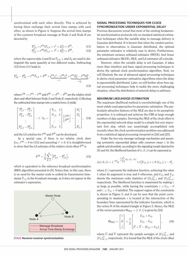
synchronized with each other directly. This is achieved byhaving them exchange their arrival time stamps with eachother, as shown in Figure 4. Suppose the arrival time stampsof the common broadcast message at Node A and Node B aredenoted by

TA2, k ¼ f PA(T1, k þ sA þ XA

k )þ hPA, (11)TB2, k ¼ f PB(T1, k þ sB þ XB

k )þ hPB, (12)

where the superscripts A and B on T2, k, s, and Xk are used to dis-tinguish the same quantity at two different nodes. Subtracting(12) from (11) leads to

TA2;k � TB

2;k ¼ f ABT1, k þ hAB þ f PAsA � f PBsB|fflfflfflfflfflfflfflfflfflffl{zfflfflfflfflfflfflfflfflfflffl}:¼s0

þ f PAXAk � f PBXB

k|fflfflfflfflfflfflfflfflfflfflffl{zfflfflfflfflfflfflfflfflfflfflffl}:¼X0

k

,

(13)

where f AB :¼ f PA � f PB and hAB :¼ hPA � hPB are the relative clockskew and offset betweenNodeA andNodeB, respectively. Collectingthe subtracted time stamps into amatrix form, it yields

TA2, 1 � TB

2, 1

TA2, 2 � TB

2, 2

..

.

TA2,N � TB

2,N

26666664

37777775� s0 � 1N ¼

T1, 1 1

T1, 2 1

..

. ...

T1,N 1

2666664

3777775

f AB

hAB

� ��

X01

X02

..

.

X0N

2666664

3777775, (14)

and the LS solution for f AB and hAB can be developed.As a special case, if there is no relative clock skew

[i.e., f AB ¼ 0 in (13)] and assuming s0 � 0, it is straightforwardto show that the LS estimate of the relative clock offset hAB is

hAB ¼ 1N

XNk¼1

TA2, k � TB

2, k

h i, (15)

which is equivalent to the reference broadcast synchronization(RBS) algorithm presented in [9]. Notice that, in this case, thereis no need for the master node to embed its transmission time-stamp T1, k in the broadcast message, as it does not appear in theestimator’s expression.

SIGNAL PROCESSING TECHNIQUES FOR CLOCKSYNCHRONIZATION UNDER EXPONENTIAL DELAYPrevious discussions reveal that most of the existing fundamen-tal synchronization protocols rely on standard statistical estima-tion techniques when the variable delay in message delivery isGaussian distributed. It is known that when the random pertur-bation in observations is Gaussian distributed, the optimalparameter estimator is relatively easy to derive. Furthermore,the minimum variance unbiased estimator (MVUE), best linearunbiased estimator (BLUE), MLE, and LS estimator all coincide.

However, when the variable delay is not Gaussian, it takesmore than intuition and basic signal processing techniques toderive the optimal clock synchronization algorithm. Next, wewill illustrate the use of advanced signal processing techniquesto derive clock parameter estimation algorithms when the delayis exponentially distributed. Later, we will further show how sig-nal processing techniques help to tackle the more challengingsituation, when the distribution of network delays is arbitrary.

MAXIMUM LIKELIHOOD ESTIMATIONThe maximum likelihood method is overwhelmingly one of themost widely used approaches for parameter estimation. The par-ticularly attractive features of the MLE are due to its asymptoticproperties: it is unbiased and achieves the CRB at large enoughnumbers of data samples. Deriving the MLE of the clock offset inthe exponential network delay model is a simple but very impor-tant first step, which was surprisingly accomplished onlyrecently when the clock synchronization problem was addressedfrom a statistical signal processing viewpoint in [24] and [25].

Under the two-way message exchange mechanism and assum-ing symmetric exponential delays with common mean k in theuplink and downlink, according to the signaling model depicted by(5) and (6), the likelihood function of (s, h, k) can be expressed as

L(s, h, k) ¼ k�2Ne�1a

PNk¼1

(UkþVk�2s)3 I U(1) � sþ h;V(1) � s� h� �

,

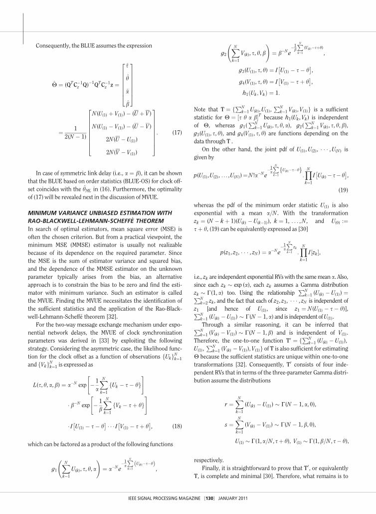
where I½�� represents the indicator function, achieving the value1 when its argument is true and 0 otherwise, and U(1) and V(1)denote the minimum order statistics of fUkgNk¼1 and fVkgNk¼1,respectively. The likelihood function is maximized by making sas large as possible, while having the constraints s � U(1) � hand s � V(1) þ h satisfied. The support region of the constraintsis shown in Figure 5, and it can be seen that the point corre-sponding to maximum s is located at the intersection of theboundary lines represented by the indicator functions, which isthe vertex M of the shaded triangle in Figure 5. Hence, the MLEof the vector parameterHMLE ¼ ½s h k� is given by [24]

HMLE ¼s

h

k

26643775 ¼ 1

2

U(1) þ V(1)

U(1) � V(1)

U þ V � (U(1) þ V(1))

2664

3775, (16)

where U and V represent the sample averages of fUkgNk¼1 andfVkgNk¼1, respectively. It is found that the MLE of the clock offset

Master Node

Node BNode A

Message Broadcast

Arrival Time-Stamp Exchange

[FIG4] Receiver-receiver synchronization.


hML coincides with the minimum round delay estimator previ-ously proposed by [12] through informal arguments. Interest-ingly, in the general case of asymmetric link delays, the MLE ofclock offset h assumes the same expression.

When the clock skew is also taken into account as in (2)and (3), there is no closed-form expression available for thejoint estimates of clock parameters under exponential linkdelays. Instead, the optimization problem is solved by maxi-mizing the likelihood function over nonlinear constraintsthrough iterative methods and it has been addressed in [26] inthe case of symmetric exponentially distributed delays. A moreelegant method to find the MLE of the clock offset and skewwas presented in [27], which utilizes the concept of profilelikelihood whereby not only the five-dimensional optimiza-tion problem is reduced to a one-dimensional problem butalso the general asymmetric delay case can be handled.Another way to get around the high-dimensional maximiza-tion of the likelihood function is to note that adding (2) and(3) eliminates the fixed delay. Then, the MLE for the clock off-set and skew can be easily derived from the resultant equation[28]. On the other hand, under the RBS protocol, [29] derivesthe joint MLE for clock offset and skew under the exponentialdelay model, and the Gibbs sampler is proposed to maximizethe likelihood function.

BEST LINEAR UNBIASED ESTIMATIONUSING ORDER STATISTICSIn many practical applications, it is difficult or impossible to findan optimal estimator due to various reasons. In such scenarios,a commonly applied methodology is to restrict the estimator tobe linear in the data and find an unbiased linear estimator withminimum variance. This results in the BLUE.

It is known that when the observation noise is Gaussian dis-tributed, BLUE provides the optimal solution by virtue of theGauss-Markov theorem. For other distributions, including theexponential distribution, direct application of BLUE cannotguarantee any optimality. However, inspired by the results thatMLE under exponentially distributed delays depends heavily onthe order statistics of the observation data, [30] derived BLUE,which later turned out to possess certain optimality features.

Now assume the two-way message exchange model and thegeneral set-up of exponential network delays for the uplink anddownlink of possibly different means, denoted by a and b,respectively. Define

U 0k :¼

1a(Uk � s� h),

V 0k :¼

1b(Vk � sþ h)

as a set of independent observations on the standardized variate.Hence, their distribution will be parameter free. Furthermore,let fU 0

kgNk¼1 and fV 0kgNk¼1 be the order statistics of fU 0

kgNk¼1 andfV 0

kgNk¼1, respectively. Using standard results for the exponentialdistribution [31, p. 500], the N 3N symmetric positive-definitecovariance matrix C for both ½U 0

ð1Þ U0ð2Þ . . . U

0ðNÞ�T and

½V 0(1) V

0(2) . . . V

0(N)�T takes the common expression

C ¼

1N2

1N2 � � � 1

N2

1N2

1N2 þ 1

(N�1)2� � � 1

N2 þ 1(N�1)2

..

. ... � � � ..

.

1N2

1N2 þ 1

(N�1)2� � � PN

k¼1

1(N�kþ1)2

26666664

37777775,

and the inverse C�1 could also be expressed in closed form.LetH :¼ ½s h a b�T be the 43 1 vector of unknown parame-

ters and z :¼ ½U(1)U(2) . . .U(N)V(1)V(2) � � � V(N)�T . Then, exploitingthe following relations

E U(k)� � ¼ sþ hþ a E U 0

(k)

h i, E V(k)� � ¼ s� hþ bE V 0

(k)

h i,

var U(k)� � ¼ a2var U 0

(k)

h i, var V(k)

� � ¼ b2var V 0(k)

h i,

cov U(k)U(j)� � ¼ a2cov U 0

(k)U0(j)

h i, cov V(k)V(j)

� � ¼ b2cov V 0(k)V

0(j)

h i,

the mean and covariance matrix of the ordered observations z isexpressed in the equation at the bottom of the page.

E z½ � ¼

1 1 � � � 1 1 1 � � � 11 1 � � � 1 �1 �1 � � � �1

1N

1N þ 1

N�1 � � � PNk¼1

1(N�kþ1) 0 0 � � � 0

0 0 � � � 0 1N

1N þ 1

N�1 � � � PNk¼1

1(N�kþ1)

266666664

377777775

T

s

h

a

b

266664

377775

:¼ QH,

E zzH� �

:¼ Cz ¼ a2C 00 b2C

� �:

V(1) + θ

–V(1) U(1)

U(1) – θ

Mτ

θ

[FIG5] Support region for the likelihood function of clockoffset estimation under exponential delays.


Consequently, the BLUE assumes the expression

H ¼ (QTC�1z Q)�1QTC�1

z z ¼

s

h

a

b

26666664

37777775

¼ 12(N � 1)

N(U(1) þ V(1))� (U þ V )

N(U(1) � V(1))� (U � V )

2N(U � U(1))

2N(V � V(1))

266666664

377777775: (17)

In case of symmetric link delay (i.e., a ¼ b), it can be shownthat the BLUE based on order statistics (BLUE-OS) for clock off-set coincides with the hML in (16). Furthermore, the optimalityof (17) will be revealed next in the discussion of MVUE.

MINIMUM VARIANCE UNBIASED ESTIMATION WITHRAO-BLACKWELL-LEHMANN-SCHEFF�E THEOREMIn search of optimal estimators, mean square error (MSE) isoften the chosen criterion. But from a practical viewpoint, theminimum MSE (MMSE) estimator is usually not realizablebecause of its dependence on the required parameter. Sincethe MSE is the sum of estimator variance and squared bias,and the dependence of the MMSE estimator on the unknownparameter typically arises from the bias, an alternativeapproach is to constrain the bias to be zero and find the esti-mator with minimum variance. Such an estimator is calledthe MVUE. Finding the MVUE necessitates the identification ofthe sufficient statistics and the application of the Rao-Black-well-Lehmann-Scheff�e theorem [32].

For the two-way message exchange mechanism under expo-nential network delays, the MVUE of clock synchronizationparameters was derived in [33] by exploiting the followingstrategy. Considering the asymmetric case, the likelihood func-tion for the clock offset as a function of observations fUkgNk¼1

and fVkgNk¼1 is expressed as

L(s, h, a, b) ¼ a�N exp � 1a

XNk¼1

Uk � s� hf g" #

� b�N exp � 1b

XNk¼1

Vk � sþ hf g" #

� I U(1) � s� h� � � � � I V(1) � sþ h

� �, (18)

which can be factored as a product of the following functions

g1XNk¼1

U(k), s, h, a

!¼ a�Ne

�1a

PNk¼1

U(k)�s�hð Þ,

g2XNk¼1

V(k), s, h, b

!¼ b�Ne

�1b

PNk¼1

(V(k)�sþh),

g3(U(1), s, h) ¼ I U(1) � s� h� �

,

g4(V(1), s, h) ¼ I V(1) � sþ h� �

,

h1 Uk;Vkð Þ ¼ 1:

Note that T ¼ fPNk¼1 U(k),U(1),

PNk¼1 V(k), V(1)g is a sufficient

statistic for H ¼ ½s h a b�T because h1(Uk, Vk) is independentof H, whereas g1(

PNk¼1 U(k), s, h, a), g2(

PNk¼1 V(k), s, h, b),

g3(U(1), s, h), and g4(V(1), s, h) are functions depending on thedata through T .

On the other hand, the joint pdf of U(1),U(2), � � � ,U(N) isgiven by

p(U(1),U(2), . . . ,U(N))¼N !a�Ne�1a

PNk¼1

U(k)�s�hf g:YNk¼1

I U(k)� s�h� �

,

(19)

whereas the pdf of the minimum order statistic U(1) is alsoexponential with a mean a=N . With the transformationzk ¼ (N � kþ 1)(U(k) � U(k�1)), k ¼ 1, . . . ,N , and U(0) :¼sþ h, (19) can be equivalently expressed as [30]

p(z1, z2, � � � , zN ) ¼ a�Ne�1a

PNk¼1

zk:YNk¼1

I zk½ �,

i.e., zk are independent exponential RVs with the samemean a. Also,since each zk � exp (a), each zk assumes a Gamma distributionzk � C(1, a) too. Using the relationship

PNk¼1 (U(k) � U(1)) ¼PN

k¼2 zk, and the fact that each of z2, z3, � � � , zN is independent ofz1 [and hence of U(1), since z1 ¼ N(U(1) � s� h)],PN

k¼1 (U(k) � U(1)) � C(N � 1, a) and is independent ofU(1).Through a similar reasoning, it can be inferred thatPNk¼1 (V(k) � V(1)) � C(N � 1, b) and is independent of V(1).

Therefore, the one-to-one function T0 ¼ fPNk¼1 (U(k) � U(1)),

U(1),PN

k¼1 (V(k) � V(1)),V(1)g of T is also sufficient for estimatingH because the sufficient statistics are unique within one-to-onetransformations [32]. Consequently, T0 consists of four inde-pendent RVs that in terms of the three-parameter Gamma distri-bution assume the distributions

r ¼XNk¼1

(U(k) � U(1)) � C(N � 1, a, 0),

s ¼XNk¼1

(V(k) � V(1)) � C(N � 1, b, 0),

U(1) � C(1,a=N , sþ h), V(1) � C(1,b=N , s� h),

respectively.Finally, it is straightforward to prove that T0, or equivalently

T, is complete and minimal [30]. Therefore, what remains is to


find an unbiased estimator for H as a function of T, which isalso the MVUE according to Rao-Blackwell-Lehmann-Scheff�etheorem. Since the BLUE-OS in (17) is such an unbiasedestimator of H as a function of T and for this reason, it is theMVUE too.

MLE VERSUS MVUE IN MSEFrom our previous discussion, it follows that, for asymmetricexponential delays in the uplink and downlink with differentmeans, the MVUE is given by

hMVUE ¼ N(U(1) � V(1))� (�U � �V )2(N � 1)

, (20)

while the MLE is hMLE ¼ (U(1) � V(1))=2. One may wonder whichestimator is better in terms ofMSE? To answer this question,note that the MVUE is notnecessarily the best estimator.It is only the best amongunbiased estimators. If a biasedestimator is devised havingreduced variance relative toMVUE at the price of an insignificant increase in its squared bias,then the biased estimator might outperform the MVUE in theMSE sense.

For the considered modeling setup, the MSEs of the MVUEand MLE can be expressed in closed form, respectively, as

MSE(hMVUE) ¼ 14N(N � 1)

(a2 þ b2),

MSE(hMLE) ¼ 12N2 (a

2 þ b2 � ab):

The MLE performs better than MVUE in the MSE sense whenMSE(hMVUE) > MSE(hMLE), or equivalently

N2� 15

ab

(a� b)2:

From the above equation, it can be seen that the MLE is betterthan the MVUE when the means of the uplink and downlinkdelays are very close to each other. Otherwise, the MVUE is bet-ter. This observation is illustrated in Figure 6, in which N ¼ 15,a ¼ 2, and b is varied across the interval ½a� 2, aþ 2�.

REMARK 3Notice that most of the techniques in this section were proposedin the context of the two-way message exchange mechanism.Since after performing a mild approximation, the system ofequations for the one-way message dissemination becomes lin-ear [see (10)], the analysis of the one-way message disseminationframework under the exponential delay model generates similarresults to those corresponding to the two-way messageexchange mechanism. For receiver–receiver synchronization,

only [29] derives the joint MLE for clock offset and skew. Thederivation of estimators assuming other optimization criteria(e.g., MVUE and BLUE) in the exponential delay environment isan interesting research topic for future studies.

SIGNAL PROCESSING TECHNIQUES FORDELAYS WITH ARBITRARY DISTRIBUTIONIn synchronizing the clocks in a WSN, it might happen thatthe underlying pdf of the network delay model is not knownin advance, and, hence, the performance of estimators spe-cially designed for a particular distribution can vary a lot.Therefore, there is a need for developing statistical signalprocessing estimation techniques that are robust to theunknown network delay distributions or can adapt to dif-ferent delay distributions. In this section, we consider three

such statistical signal pro-cessing techniques.

LINEAR PROGRAMMINGESTIMATIONA linear programming (LP)problem is defined as the prob-lem of maximizing or minimiz-

ing a linear function subject to linear equality or inequalityconstraints. For the one-way message dissemination scheme,note from (10) that if the link delays are coming from a nonnega-tive distribution, estimation of clock skew and offset can be castas a linear program

minimizeXNk¼1

(T2, k � T1, kf � h),

subject to h � T2, k � T1, kf 8 k ¼ 1, 2, . . . ,N :

The above linear program can be solved through many differenttechniques such as the simplex algorithm, ellipsoid method, orinterior point methods. The solution to this linear program givesthe ML estimate if the transmission delays are exponentially

0 0.5 1 1.5 2 2.5 3 3.5 40

0.005

0.01

0.015

0.02

0.025

0.03

β = (α − r/2) : (α + r/2)

MS

E

α = β

MVUEMLE

[FIG6] TheMSE of the MLE andMVUE under different a and b.

TWO-WAYMESSAGE EXCHANGE IS ACLASSICALMECHANISM FOR

EXCHANGING TIMING INFORMATIONBETWEEN TWOADJACENT NODES.


distributed. Even if the delaydistribution is not exponential,it is quite logical to use a linearprogram to estimate the clockparameters, and, hence, thisapproach was elegantly put for-ward in [11]. LP was alsoemployed to solve the clock synchronization problem in the con-text of wireless ad hoc networks based on the one-way messagedisseminationmechanism in [34].

On the other hand, clock synchronization under the two-waymessage exchange mechanism can also be cast into the LP prob-lem [35]. From (2) and (3), we can write

1fT2, k � h

f� (sþ Xk) ¼ T1, k,

1fT3, k � h

fþ (sþ Yk) ¼ T4, k:

Assuming Node B replies Node A immediately (see Figure 2)after receiving the timing message (i.e., T2, k ¼ T3, k), and thedelays s, Xk, and Yk are nonnegative, the above two equationscan be represented in terms of the constraints:T1, k � fT2, k � h0 � T4, k, where f 0 :¼ 1=f and h0 :¼ h=f . It isproposed in [35] that the upper limit of the optimal set-valuedestimate of f 0 is given by the following linear program

maxf 0;h0

½f 0h0� 10

� �,

subject to T1,k � f 0T2,k � h0 � T4,k 8 k ¼ 1, 2, . . . ,N ,

ð21Þ

and a lower limit estimate of f 0 is given by a similar linear pro-gram, but with maximization replaced by minimization. Sup-pose (f 0, h01) is the solution for (21) and (f 0, h02) is the solution forthe same linear program but with minimization, [35] provesthat ½f 0; f 0�3 ½h0; h0� is a consistent set-valued estimate that mini-mizes the product (f 0 � f 0)(h0 � h0) where h0 :¼ max (h01, h

02) and

h0 :¼ min (h01, h02).

BOOTSTRAP BIAS CORRECTIONBootstrap is an approach for statistical inference based on build-ing a sampling distribution for a statistic by resampling fromthe data at hand (see, e.g., [36] and [37]). For small sample sizes,such a method is usually superior to large sample techniques.On the downside, its computational complexity is considerablygreater than the standard techniques described earlier in thisarticle. We now discuss the application of bootstrap bias correc-tion in the context of clock offset estimation.

Bootstrap bias correction typically reduces the bias of an esti-mator at the expense of increased variance but with an overalleffect of reduced MSE. As explained in [38], suppose thatan unknown probability distribution F assumes the datax ¼ (x1, x2, � � � , xN ) by random sampling. We want to estimate areal-valued parameter h. For now, we will assume the estimator

to be any statistic h ¼ s(x). Thebias of h ¼ s(x) is defined to bethe difference between theexpectation of h and the valueof the parameter h, B(h) ¼EF ½s(x)� � h. In practice, wemay not know the distribution

F or the true value of h, so B(h) cannot be computed. However,we can approximate the bias with the bootstrap estimate, whichis defined as

B(h) ¼ EF ½s(x)� � h, (22)

where F is the empirical distribution constructed from x. Tocompute EF ½s(x)�, we generate independent bootstrap samplesx�1, x�2, . . . , x�M from F, evaluate the bootstrap replicationsh�(m) ¼ s(x�m), and approximate the bootstrap expectationEF ½s(x�)� by the average

EF ½s(x)� ¼1M

XMm¼1

s(x�m):

Therefore, the bias-corrected estimator is

hBC ¼ h� B(h) ¼ 2h� 1M

XMm¼1

s(x�m):

In the context of clock synchronization, two sensor nodesexchange timing packets to obtain the data sets fUkgNk¼1 andfVkgNk¼1, as defined in (5) and (6), and suppose the estimatorunder consideration is h ¼ s(fUkgNk¼1, fVkgNk¼1). For the non-parametric bootstrap method, the empirical distributions offUkgNk¼1 and fVkgNk¼1, denoted by F and G, are constructed.From F and G, the samples fU�

1 ,U�2 , � � � ,U�

Ng andfV�

1 , V�2 , � � � , V �

Ng, called the bootstrap resamples, are redrawn.Then, the distribution of h is approximated by the empiricaldistribution of h� ¼ s(fU�

k gNk¼1, fV�k gNk¼1) derived from the boot-

strap resamples.In case when some partial information about the true distri-

butions of fUkgNk¼1 and fVkgNk¼1, denoted by F and G, is avail-able, the parametric bootstrap technique can be applied. Forexample, if F and G are known to obey a particular distributionbut with unknown mean l, we should draw resamples from thatdistribution with mean l, where l is estimated from the samplesfUkgNk¼1 and fVkgNk¼1.

It must be emphasized that not all bootstrap bias-correctedestimators have to be evaluated via resampling methods. It isinteresting to observe that [39] derives a closed-form expres-sion for the bootstrap bias corrected estimator for clock offsetin the two-way message exchange scenario. From (5) and (6),the marginal distributions of Uk and Vk are defined asF(u) :¼ F(u� h� s) and G(v) :¼ G(vþ h� s), respectively,and it is assumed that F(u) and G(v) are nonnegative such thatUk � hþ s and Vk�� hþ s hold. Moreover, their joint distri-bution is H(u, v) ¼ F(u)G(v) due to the independence of the

THEMAXIMUM LIKELIHOODMETHODIS OVERWHELMINGLY ONE OF THEMOSTWIDELY USED APPROACHESFOR PARAMETER ESTIMATION.


transmission delays in bothdirections. The nonparametricestimator of H(u, v) isH(u, v) ¼ F(u)G(v), whereF(u) and G(v) are the empiricalprobability distributions basedon the observations fUkgNk¼1

and fVkgNk¼1, respectively.Assume that the bias of the

MLE hML ¼ (U(1) � V(1))=2when applied to unknown distributions F andG is of interest

B(hML) ¼ 12EH(U(1) � V(1))� h

¼ 12

Z10

1� F(u)½ �Ndu�Z10

1� G(v)½ �Ndv0@

1A� h:

The bootstrap estimate of this bias is

B(hML) ¼ 12

Z10

1� F(u)h iN

du�Z10

1� G(v)h iN

dv

0@

1A� hML:

Now defining U(0) ¼ V(0) ¼ 0 and U(Nþ1) ¼ V(Nþ1) ¼ 1, we canwrite

1� F(u) ¼XNþ1

k¼1

N � kþ 1N

I U(k�1) �u�U(k)� �

,

1� G(v) ¼XNþ1

k¼1

N � kþ 1N

I V(k�1) � v�V(k)� �

:

From the above three equations, it can be shown that

B(hML) ¼ 12

XNk¼1

N � kþ 1N

� �N

� N � kN

� �N( )

3 (U(k) � V(k))� hML:

Finally, a bias-corrected estimator can be expressed as

hBC ¼ hML� B(hML)

¼U(1)�V(1)�12

XNk¼1

N�kþ1N

� �N

� N�kN

� �N( )

(U(k)�V(k)):

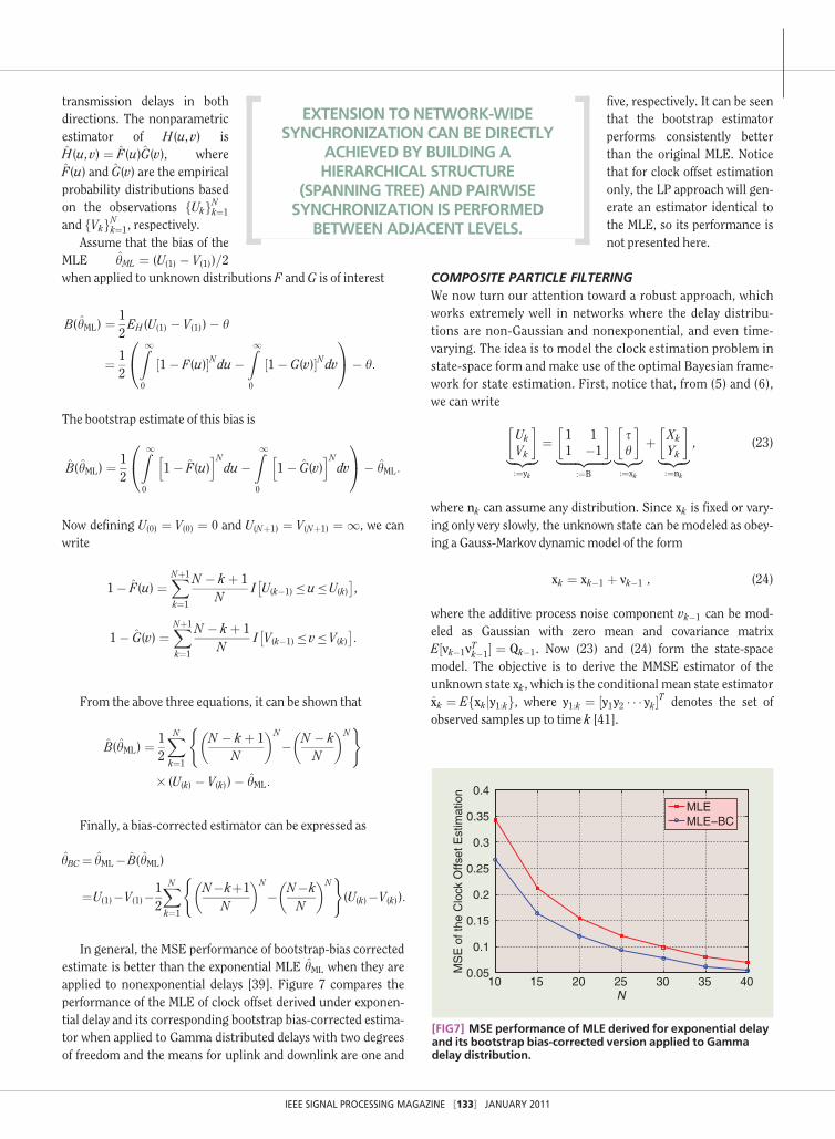
In general, the MSE performance of bootstrap-bias correctedestimate is better than the exponential MLE hML when they areapplied to nonexponential delays [39]. Figure 7 compares theperformance of the MLE of clock offset derived under exponen-tial delay and its corresponding bootstrap bias-corrected estima-tor when applied to Gamma distributed delays with two degreesof freedom and the means for uplink and downlink are one and

five, respectively. It can be seenthat the bootstrap estimatorperforms consistently betterthan the original MLE. Noticethat for clock offset estimationonly, the LP approach will gen-erate an estimator identical tothe MLE, so its performance isnot presented here.

COMPOSITE PARTICLE FILTERINGWe now turn our attention toward a robust approach, whichworks extremely well in networks where the delay distribu-tions are non-Gaussian and nonexponential, and even time-varying. The idea is to model the clock estimation problem instate-space form and make use of the optimal Bayesian frame-work for state estimation. First, notice that, from (5) and (6),we can write

UkVk

� �|fflffl{zfflffl}:¼yk

¼ 1 11 �1

� �|fflfflfflfflfflffl{zfflfflfflfflfflffl}

:¼B

sh

� �|ffl{zffl}:¼xk

þ XkYk

� �|fflffl{zfflffl}:¼nk

, (23)

where nk can assume any distribution. Since xk is fixed or vary-ing only very slowly, the unknown state can be modeled as obey-ing a Gauss-Markov dynamic model of the form

xk ¼ xk�1 þ vk�1 , (24)

where the additive process noise component vk�1 can be mod-eled as Gaussian with zero mean and covariance matrixE½vk�1vTk�1� ¼ Qk�1. Now (23) and (24) form the state-spacemodel. The objective is to derive the MMSE estimator of theunknown state xk, which is the conditional mean state estimatorxk ¼ Efxkjy1:kg, where y1:k ¼ ½y1y2 � � � yk�T denotes the set ofobserved samples up to time k [41].

10 15 20 25 30 35 400.05

0.1

0.15

0.2

0.25

0.3

0.35

0.4

N

MS

E o

f th

e C

lock O

ffset E

stim

ation

MLE

MLE−BC

[FIG7] MSE performance of MLE derived for exponential delayand its bootstrap bias-corrected version applied to Gammadelay distribution.

EXTENSION TO NETWORK-WIDESYNCHRONIZATION CAN BE DIRECTLY

ACHIEVED BY BUILDING AHIERARCHICAL STRUCTURE

(SPANNING TREE) AND PAIRWISESYNCHRONIZATION IS PERFORMED

BETWEEN ADJACENT LEVELS.


The optimal state estimationconsists of two main steps: timeupdate andmeasurement update.Suppose at time k� 1, the poste-rior distribution p(xk�1jy1:k�1) isknown, the time update stepresumes to obtain the predictivedistribution

p(xkjy1:k�1) ¼Z

p(xkjxk�1)p(xk�1jy1:k�1)dxk�1, (25)

where the transition density p(xkjxk�1) is related to the statetransition equation (24). On the other hand, in the measure-ment update step, based on the new observation yk and thepredictive distribution p(xkjy1:k�1), the marginal posteriordistribution of state at time k is obtained as

p(xkjy1:k) ¼ Ckp(xkjy1:k�1)p(ykjxk) , (26)

where

Ck ¼Z

p(xkjy1:k�1)p(ykjxk)dxk� ��1

(27)

is a normalization constant and p(ykjxk) is the likelihood of theobservation yk given xk and is related to the observation equation(23). In general, when the model is linear with Gaussian noiseand the prior knowledge about the initial state x0 is Gaussian, theKalman filter provides the mean and covariance update sequen-tially and is the optimal Bayesian solution. If the noise is notGaussian, there may not be closed-form expression to (25) and(26), and particle filtering [40], in which a set of particles with

weights are used to approximatethe shape of the distribution,becomes an attractive alterna-tive to the closed-form solution.

In the composite particle fil-tering, the predictive and poste-rior distributions are modeledby Gaussian mixture models[40], and each component is

updated using the Kalman filter or particle filter. This solutionpresents a smaller computational complexity than a pure particlefilter solution, as the procedure called resampling is avoided [40].More specifically, let the posterior distribution at time k� 1assume the following decomposition

p(xk�1jy1:k�1) �XGg¼1

w(k�1)gN (xk�1;l(k�1)g,P(k�1)g), (28)

where G is the number of mixing components, w(k�1)g is themixing weight, andN (x;l,P) denotes the Gaussian distributionwith mean l and covariance P. Plugging (28) into the timeupdate step (25), the predictive distribution takes the form

p(xkjy1:k�1) ¼XG

g¼1

w(k�1)g

Zp(xkjxk�1)N (xk�1; l(k�1)g,P(k�1)g)dxk�1: (29)

Since the state transition (24) is linear and the noise vk�1 isGaussian distributed, the predictive distribution can be obtainedby a bank ofGKalman filters and the result is [40]

p(xkjy1:k�1) �XGg¼1

�wkgN (xk; �lkg, �Pkg), (30)

where �wkg ¼ w(k�1)g, �lkg ¼ l(k�1)g and �Pkg ¼ P(k�1)g þ Qk�1.After obtaining the predictive distribution and plugging it

into the measurement update equation (26), it follows that

p(xkjy1:k) ¼ Ck

XGg¼1

�wkgp(ykjxk)N (xk; �lkg, �Pkg): (31)

Sine p(xkjy1:k) is eventually approximated by a mixture ofGaussian pdfs, each term on the right-hand side of (31) given byp(ykjxk)N (xk;�lkg, �Pkg) is approximated with a Gaussian withmean and covariance calculated using samples obtained fromimportance sampling. Suppose the J samples generated fromeach p(ykjxk)N (xk;�lkg, �Pkg) are x(j)kg with the correspondingweighting factors c(j)kg(j ¼ 1, . . . , J). Then, the updated mean andcovariance of each of the G components are given by

lkg ¼XJj¼1

c(j)kgx(j)kg=XJj¼1

c(j)kg , (32)

Pkg ¼XJj¼1

c(j)kg(x(j)kg � lkg)(x

(j)kg � lkg)

T=XJj¼1

c(j)kg: (33)

5 10 15 20 25

101

100

10–1

10–2

10–3

10–4

N

MS

E o

f C

lock O

ffset E

stim

ation

MLE for Symmetric Gaussian Delay

MLE for Symmetric Exponential Delay

Composite Particle Filter

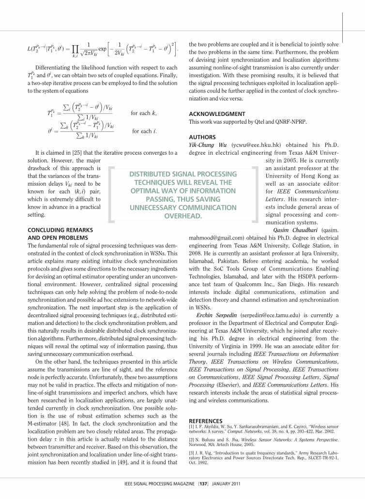
[FIG8] MSE performance of MLEs derived for Gaussian andexponential delays, and the composite particle filter, appliedto Gamma delay distribution.

CENTRALIZED SIGNAL PROCESSINGTECHNIQUES CAN ONLY HELP

SOLVING THE PROBLEMOF NODE-TO-NODE SYNCHRONIZATION AND

POSSIBLE AD HOC EXTENSIONS TONETWORK-WIDE SYNCHRONIZATION.


Then, the posterior distribution is given by

p(xkjy1:k) �XGg¼1

wkgN (xk; lkg,Pkg) , (34)

where wkg ¼ ~wkg=PG

g¼1 ~wkg and ~wkg ¼ �wkgPJ

j¼1 c(j)kg=

(PG

g¼1PJ

j¼1 c(j)kg).

Finally, the conditional mean state estimate and the corre-sponding error covariance are calculated as follows:

xk ¼XGg¼1

wkglkg, Pk ¼XGg¼1

wkg(Pkg þ (xk � lkg)(xk � lkg)T �:

It should be noted that the composite particle filter-ing approach allows tracking of time-varying clock off-set, which represents a more realistic model than aconstant phase.

Figure 8 compares the performance of the MLEs of clock off-set derived under symmetric Gaussian and exponential delaysand the composite particle filter. The message delivery delay isGamma distributed with two degrees of freedom, and the meansfor uplink and downlink are two and one, respectively. For thecomposite particle filter, Q ¼ 10�4I, the number of particles andGaussian mixture model components are 100 and three, respec-tively. It can be seen that the composite particle filter performsmuch better than the MLEs derived under the symmetric Gaus-sian or exponential delay assumption. This comes at the expenseof increased computational complexity and knowledge of theobservation noise.

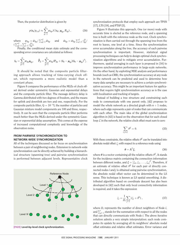
FROM PAIRWISE SYNCHRONIZATION TONETWORK-WIDE SYNCHRONIZATIONAll of the techniques discussed so far focus on synchronizationbetween a pair of neighboring nodes. Extension to network-widesynchronization can be directly achieved by building a hierarch-ical structure (spanning tree) and pairwise synchronizationis performed between adjacent levels. Representative clock

synchronization protocols that employ such approach are TPSN[17], LTS [19], and FTSP [5].

Figure 9 illustrates this approach. One (or more) node withaccurate time is elected as the reference node, and a spanningtree is built with the reference node as the root. Clock synchro-nization is then carried out through the spanning tree from theroot to leaves, one level at a time. Since the synchronizationerror accumulates along the tree, the accuracy of each pairwisesynchronization is important. However, statistical signalprocessing techniques can help to design optimal clock synchro-nization algorithms and to mitigate error accumulation. Fur-thermore, spatial averaging in each layer is proposed in [16] toimprove synchronization performance in large-scale networks.On the other hand, by exploiting MSE analysis and performancebounds (such as CRB), the synchronization accuracy at any nodein the network can be predicted and used to determine howmany data samples are necessary to achieve a certain synchroni-zation accuracy. This might be an important feature for applica-tions that require tight synchronization accuracy as is the casewith localization and tracking of targets.

Instead of building a tree structure and constraining eachnode to communicate with one parent only, [42] proposes tomodel the whole network as a directed graph with nþ 1 nodes,where each edge represents a pair of nodes that can communicatewith each other. The main idea of the global synchronizationalgorithm in [42] is based on the observation that for each closedloopL in the network, the relative clock offset must sum to zero

Xi, j2L

hij ¼ 0: (35)

With these constraints, the relative offsets hij can be translated intoabsolute nodal offset nj with respect to a reference node using

h ¼ ATn, (36)

where h is a vector containing all the relative offsets hij, A standsfor the incidence matrix containing the connection informationbetween different nodes, and n ¼ ½n0, n1, . . . , nn�T . Therefore, ifan estimate of relative offset hij for each pair of directly con-nected nodes i and j is obtained using pairwise synchronization,the absolute nodal offset vector can be determined in the LSsense. This technique is known as LS spatial smoothing. A dis-tributed algorithm based on coordinate descent has also beendeveloped in [42] such that only local connectivity informationis required, and it takes the expression

ni ¼1Di

Xj$i

(nj þ hji) , (37)

where Di represents the number of direct neighbors of Node i,and

Pj$i stands for the summation with respect to all the nodes

that can directly communicate with Node i. The above iterativesolution admits a very simple interpretation: each node com-putes its update by averaging all its neighbors’ absolute nodaloffset estimates and relative offset estimates. Error variance and

Reference Node

Level 1

Level 2

Level N

. . . . .

[FIG9] Level-by-level clock synchronization.


convergence analysis of this approach are reported in [43]. Inci-dentally, this distributed spatial smoothing algorithm coincidesin spirit with the diffusion algorithms proposed in [44]. Recently,a distributed synchronization technique based on coupled phase-locked loops (PLLs) [15] also assumes the interpretation of spatialaveraging. Furthermore, in the terminology of PLLs, the clocksynchronization algorithms proposed herein could be interpretedas the optimal way of deriving the time error detector.

In addition to building a tree and spatial smoothing, morerecently, a new approach called pairwise broadcast synchroniza-tion (PBS) was introduced in [45]. This approach allows a sensorto synchronize itself by overhearing timing messages from aneighboring two-way message exchange without sending outany packet itself. In a one-hop sensor network where every nodeis a neighbor of each other, a single PBS message exchangebetween two nodes would facil-itate all nodes to synchronize,thus significantly reducing thecommunication overhead forachieving clock synchroniza-tion. Further extensions of PBSto multihop scenarios were alsodiscussed in [46] and [47].

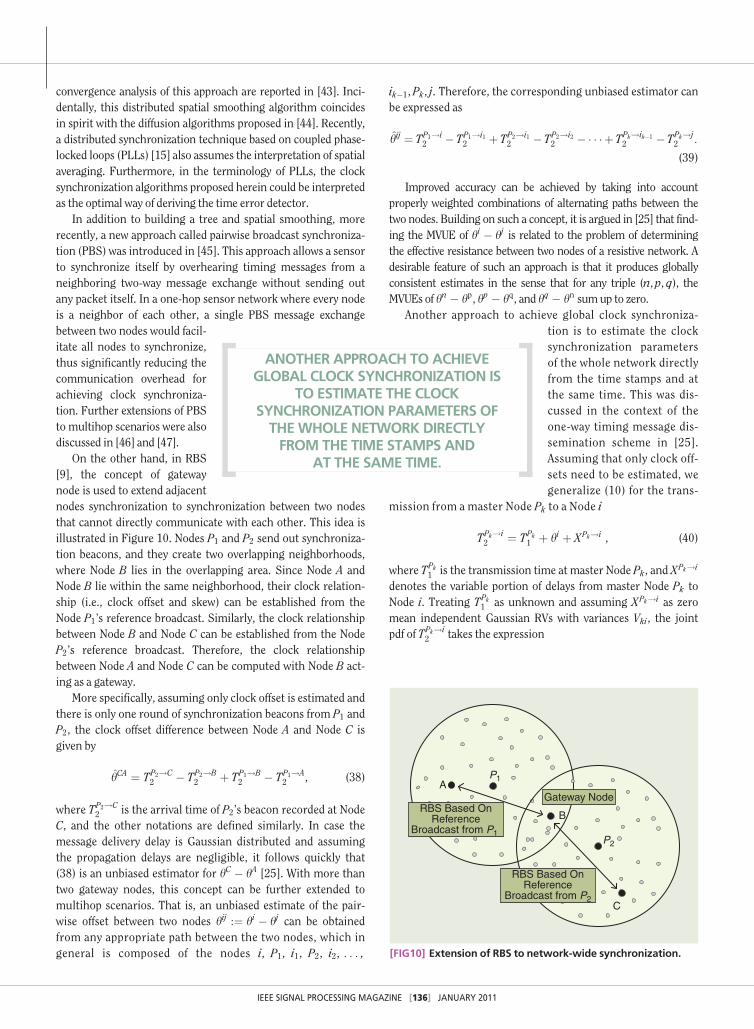
On the other hand, in RBS[9], the concept of gatewaynode is used to extend adjacentnodes synchronization to synchronization between two nodesthat cannot directly communicate with each other. This idea isillustrated in Figure 10. Nodes P1 and P2 send out synchroniza-tion beacons, and they create two overlapping neighborhoods,where Node B lies in the overlapping area. Since Node A andNode B lie within the same neighborhood, their clock relation-ship (i.e., clock offset and skew) can be established from theNode P1’s reference broadcast. Similarly, the clock relationshipbetween Node B and Node C can be established from the NodeP2’s reference broadcast. Therefore, the clock relationshipbetween Node A and Node C can be computed with Node B act-ing as a gateway.

More specifically, assuming only clock offset is estimated andthere is only one round of synchronization beacons from P1 andP2, the clock offset difference between Node A and Node C isgiven by

hCA ¼ TP2!C2 � TP2!B

2 þ TP1!B2 � TP1!A

2 , (38)

where TP2!C2 is the arrival time of P2’s beacon recorded at Node

C, and the other notations are defined similarly. In case themessage delivery delay is Gaussian distributed and assumingthe propagation delays are negligible, it follows quickly that(38) is an unbiased estimator for hC � hA [25]. With more thantwo gateway nodes, this concept can be further extended tomultihop scenarios. That is, an unbiased estimate of the pair-wise offset between two nodes hij :¼ hi � hj can be obtainedfrom any appropriate path between the two nodes, which ingeneral is composed of the nodes i, P1, i1, P2, i2, . . . ,

ik�1, Pk, j. Therefore, the corresponding unbiased estimator canbe expressed as

hij ¼ TP1!i2 � TP1!i1

2 þ TP2!i12 � TP2!i2

2 � � � � þ TPk!ik�12 � TPk!j

2 :

(39)

Improved accuracy can be achieved by taking into accountproperly weighted combinations of alternating paths between thetwo nodes. Building on such a concept, it is argued in [25] that find-ing the MVUE of hi � hj is related to the problem of determiningthe effective resistance between two nodes of a resistive network. Adesirable feature of such an approach is that it produces globallyconsistent estimates in the sense that for any triple (n, p, q), theMVUEs of hn � hp, hp � hq, and hq � hn sumup to zero.

Another approach to achieve global clock synchroniza-tion is to estimate the clocksynchronization parametersof the whole network directlyfrom the time stamps and atthe same time. This was dis-cussed in the context of theone-way timing message dis-semination scheme in [25].Assuming that only clock off-sets need to be estimated, wegeneralize (10) for the trans-

mission from a master Node Pk to a Node i

TPk!i2 ¼ TPk

1 þ hi þ XPk!i , (40)

where TPk1 is the transmission time at master Node Pk, and XPk!i

denotes the variable portion of delays from master Node Pk toNode i. Treating TPk

1 as unknown and assuming XPk!i as zeromean independent Gaussian RVs with variances Vki, the jointpdf of TPk!i

2 takes the expression

ANOTHER APPROACH TO ACHIEVEGLOBAL CLOCK SYNCHRONIZATION IS

TO ESTIMATE THE CLOCKSYNCHRONIZATION PARAMETERS OFTHEWHOLE NETWORK DIRECTLYFROM THE TIME STAMPS AND

AT THE SAME TIME.

P1A

P2

C

B

Gateway NodeRBS Based On

ReferenceBroadcast from P1

RBS Based OnReference

Broadcast from P2

[FIG10] Extension of RBS to network-wide synchronization.


L(TPk!i2 jTPk

1 , hi) ¼Yk, i

1ffiffiffiffiffiffiffiffiffiffiffi2pVki

p exp � 12Vki

TPk!i2 � TPk

1 � hi �2� �

:

Differentiating the likelihood function with respect to eachTPk1 and hi, we can obtain two sets of coupled equations. Finally,

a two-step iterative process can be employed to find the solutionto the system of equations

TPk1 ¼

Pi TPk!i

2 � hi �

=VkiPi 1=Vki

for each k,

hi ¼P

k TPk!i2 � TPk

1

�=VkiP

k 1=Vkifor each i:

It is claimed in [25] that the iterative process converges to asolution. However, the majordrawback of this approach isthat the variances of the trans-mission delays Vki need to beknown for each (k, i) pair,which is extremely difficult toknow in advance in a practicalsetting.

CONCLUDING REMARKSAND OPEN PROBLEMSThe fundamental role of signal processing techniques was dem-onstrated in the context of clock synchronization in WSNs. Thisarticle explains many existing intuitive clock synchronizationprotocols and gives some directions to the necessary ingredientsfor devising an optimal estimator operating under an unconven-tional environment. However, centralized signal processingtechniques can only help solving the problem of node-to-nodesynchronization and possible ad hoc extensions to network-widesynchronization. The next important step is the application ofdecentralized signal processing techniques (e.g., distributed esti-mation and detection) to the clock synchronization problem, andthis naturally results in desirable distributed clock synchroniza-tion algorithms. Furthermore, distributed signal processing tech-niques will reveal the optimal way of information passing, thussaving unnecessary communication overhead.

On the other hand, the techniques presented in this articleassume the transmissions are line of sight, and the referencenode is perfectly accurate. Unfortunately, these two assumptionsmay not be valid in practice. The effects and mitigation of non-line-of-sight transmissions and imperfect anchors, which havebeen researched in localization applications, are largely unat-tended currently in clock synchronization. One possible solu-tion is the use of robust estimation schemes such as theM-estimator [48]. In fact, the clock synchronization and thelocalization problem are two closely related areas. The propaga-tion delay s in this article is actually related to the distancebetween transmitter and receiver. Based on this observation, thejoint synchronization and localization under line-of-sight trans-mission has been recently studied in [49], and it is found that

the two problems are coupled and it is beneficial to jointly solvethe two problems in the same time. Furthermore, the problemof devising joint synchronization and localization algorithmsassuming nonline-of-sight transmission is also currently underinvestigation. With these promising results, it is believed thatthe signal processing techniques exploited in localization appli-cations could be further applied in the context of clock synchro-nization and vice versa.

ACKNOWLEDGMENTThis work was supported by Qtel and QNRF-NPRP.

AUTHORSYik-Chung Wu ([email protected]) obtained his Ph.D.degree in electrical engineering from Texas A&M Univer-

sity in 2005. He is currentlyan assistant professor at theUniversity of Hong Kong aswell as an associate editorfor IEEE CommunicationsLetters. His research inter-ests include general areas ofsignal processing and com-munication systems.

Qasim Chaudhari ([email protected]) obtained his Ph.D. degree in electricalengineering from Texas A&M University, College Station, in2008. He is currently an assistant professor at Iqra University,Islamabad, Pakistan. Before entering academia, he workedwith the SoC Tools Group of Communications EnablingTechnologies, Islamabad, and later with the HSDPA perform-ance test team of Qualcomm Inc., San Diego. His researchinterests include digital communications, estimation anddetection theory and channel estimation and synchronizationin WSNs.

Erchin Serpedin ([email protected]) is currently aprofessor in the Department of Electrical and Computer Engi-neering at Texas A&M University, which he joined after receiv-ing his Ph.D. degree in electrical engineering from theUniversity of Virginia in 1999. He was an associate editor forseveral journals including IEEE Transactions on InformationTheory, IEEE Transactions on Wireless Communications,IEEE Transactions on Signal Processing, IEEE Transactionson Communications, IEEE Signal Processing Letters, SignalProcessing (Elsevier), and IEEE Communications Letters. Hisresearch interests include the areas of statistical signal process-ing and wireless communications.

REFERENCES[1] I. F. Akyildiz, W. Su, Y. Sankarasubramaniam, and E. Cayirci, ‘‘Wireless sensornetworks: A survey,’’ Comput. Networks, vol. 38, no. 4, pp. 393–422, Mar. 2002.

[2] N. Bulusu and S. Jha, Wireless Sensor Networks: A Systems Perspective.Norwood, MA: Artech House, 2005.

[3] J. R. Vig, ‘‘Introduction to quatz frequency standards,’’ Army Research Labo-ratory Electronics and Power Sources Directorate Tech. Rep., SLCET-TR-92-1,Oct. 1992.

DISTRIBUTED SIGNAL PROCESSINGTECHNIQUESWILL REVEAL THE

OPTIMALWAYOF INFORMATIONPASSING, THUS SAVING

UNNECESSARY COMMUNICATIONOVERHEAD.


[4] H. Kopetz and W. Ochsenreiter, ‘‘Clock synchronization in distributedreal-time systems,’’ IEEE Trans. Comput., vol. 36, no. 8, pp. 933–939, Aug.1987.

[5] M. Maroti, B. Kusy, G. Simon, and A. Ledeczi, ‘‘The flooding time synchroni-zation protocol,’’ in Proc. 2nd Int. Conf. Embedded Networked Sensor Systems,ACM Press, Nov. 2004, pp. 39–49.

[6] A. Papoulis, Probability, Random Variables and Stochastic Processes, 3rded. New York: McGraw-Hill, 1991.

[7] A. Leon-Garcia, Probability and Random Processes for Electrical Engineer-ing. 2nd ed. Reading, MA: Addison-Wesley, 1993.

[8] C. Bovy, H. Mertodimedjo, G. Hooghiemstra, H. Uijterwaal, and P. Mie-ghem, ‘‘Analysis of end-to-end delay measurements in Internet,’’ in Proc.Passive and Active Measurements Workshop, Fort Collins, CO, Mar. 2002,pp. 26–33.

[9] J. Elson, L. Girod, and D. Estrin, ‘‘Fine-grained network time synchroniza-tion using reference broadcasts,’’ in Proc. 5th Symp. Operating System Designand Implementation, Dec. 2002, pp. 147–163.

[10] H. S. Abdel-Ghaffar, ‘‘Analysis of synchronization algorithm with time-outcontrol over networks with exponentially symmetric delays,’’ IEEE Trans. Com-mun., vol. 50, pp. 1652–1661, Oct. 2002.

[11] S. Moon, P. Skelley, and D. Towsley, ‘‘Estimation and removal of clockskew from network delay measurements,’’ in Proc. IEEE INFOCOM, New York,Mar. 1999, pp. 227–234.

[12] V. Paxson, ‘‘On calibrating measurements of packet transit times,’’ in Proc.7th ACM Sigmetrics Conf., June 1998, pp. 11–21.

[13] G. J. Pottie and W. J. Kaiser, ‘‘Wireless integrated network sensors,’’ Com-mun. ACM, vol. 43, no. 5, pp. 51–58, May 2000.

[14] Y.-W. Hong and A. Scaglione, ‘‘A scalable synchronization protocol for largescale sensor networks and its applications,’’ IEEE JSAC, vol. 23, no. 5,pp. 1085–1099, May 2005.

[15] O. Simeone, U. Spagnolini, Y. Bar-Ness, and S. H. Strogatz, ‘‘Distributedsynchronization in wireless networks,’’ IEEE Signal Processing Mag., vol. 25,no. 5, pp. 81–97, Sept. 2008.

[16] A. Hu and S. D. Servetto. (2006). A scalable protocol for cooperative timesynchronization using spatial averaging [Online]. Available: http://arxiv.org/PScache/cs/pdf/0611/0611003v1.pdf

[17] S. Ganeriwal, R. Kumar, and M. B. Srivastava, ‘‘Timing-sync protocolfor sensor networks,’’ in Proc. SenSys 03, Los Angeles, CA, Nov. 2003,pp. 138–149.

[18] M. L. Sichitiu and C. Veerarittiphan, ‘‘Simple, accurate time synchroniza-tion for wireless sensor networks,’’ in Proc. IEEE WCNC, New Orleans, LA, Mar.2003, pp. 1266–1273.

[19] J. Van Greunen and J. Rabaey, ‘‘Lightweight time synchronization for sen-sor networks,’’ in Proc. 2nd ACM Int. Conf. Wireless Sensor Networks andApplications (WSNA), San Diego, CA, 2003, pp. 11–19.

[20] B. Sundararaman, U. Buy, and A. D. Kshemkalyani, ‘‘Clock synchronizationfor wireless sensor networks: a survey,’’ Ad-Hoc Networks, vol. 3, no. 3,pp. 281–323, Mar. 2005.

[21] K. Noh, Q. Chaudhari, E. Serpedin, and B. Suter, ‘‘Novel clock phaseoffset and skew estimation two-way timing message exchanges for wirelesssensor networks,’’ IEEE Trans. Commun., vol. 55, no. 4, pp. 766–777, Apr.2007.

[22] M. Leng and Y.-C. Wu, ‘‘On clock synchronization algorithms for wirelesssensor networks under unknown delay,’’ IEEE Trans. Veh. Technol., vol. 59,no. 1, pp. 182–190, Jan. 2010.

[23] P. Huang, M. Desai, X. Qiu, and B. Krishnamachari, ‘‘On the multihopperformance of synchronization mechanisms in high propagation delay net-works,’’ IEEE Trans. Comput., vol. 58, no. 5, pp. 577–590, May 2009.

[24] D. Jeske, ‘‘On the maximum likelihood estimation of clock offset,’’ IEEETrans. Commun., vol. 53, no. 1, pp. 53–54, Jan. 2005.

[25] R. Karp, J. Elson, C. Papadimitriou, and S. Shenker, ‘‘Global synchroniza-tion in sensornets,’’ in Proc. 6th Latin American Symp. Theoretical Informatics,Apr. 2004, pp. 609–624.

[26] Q. Chaudhari, E. Serpedin, and K. Qaraqe, ‘‘On maximum likelihood esti-mation of clock offset and skew in networks with exponential delays,’’ IEEETrans. Signal Processing, vol. 56, no. 4, pp. 1685–1697, Apr. 2008.

[27] J. Li and D. Jeske, ‘‘Maximum likelihood estimators of clock offset and skewunder exponential delays,’’ Appl. Stochastic Models Bus. Ind., vol. 25, no. 4,pp. 445–459, Apr. 2009.

[28] M. Leng and Y.-C. Wu, ‘‘On joint synchronization of clock offset and skewfor wireless sensor networks under exponential delay,’’ in Proc. IEEE ISCAS,Paris, France, May 2010, pp. 461–464.

[29] I. Sari, E. Serpedin, K.-L. Noh, Q. Chaudhari, and B. Suter, ‘‘On the jointsynchronization of clock offset and skew in RBS-protocol,’’ IEEE Trans. Com-mun., vol. 56, no. 5, pp. 700–703, May 2008.

[30] Q. Chaudhari, E. Serpedin, and K. Qaraqe, ‘‘On minimum varianceunbiased estimation of clock offset in distributed networks,’’ IEEE Trans.Inform. Theory, vol. 56, no. 6, pp. 2893–2904, June 2010.

[31] N. Johnson, S. Kotz, and N. Balakrishnan, Continuous Univariate Distribu-tions, 2nd ed. New York: Wiley, vol. 1, 1994.

[32] S. M. Kay, Fundamentals of Statistical Signal Processing, Vol. I. Estima-tion Theory. Englewood Cliffs, NJ: Prentice-Hall, 1993.

[33] Q. Chaudhari, E. Serpedin, and Y.-C. Wu, ‘‘Improved estimation of clockoffset in sensor networks,’’ in Proc. IEEE Int. Conf. Communications (ICC),Dresden, Germany, June 2009, pp. 1–4.

[34] B. Scheuermann, W. Kiess, M. Roos, M. Mauve, and F. Jarre, ‘‘On the timesynchronization of distributed log files in networks with local broadcast media,’’IEEE/ACM Trans. Networking, vol. 17, no. 2, pp. 431–444, Apr. 2009.

[35] M. Lemmon, J. Ganguly, and L. Xia, ‘‘Model-based clock synchronization innetworks with drifting clocks,’’ in Proc. Pacific Rim Int. Symp. DependableComputing, Los Angeles, CA, pp. 177–184, Dec. 2000.

[36] B. Efron and R. J. Tibshirani, An Introduction to the Bootstrap. London:U.K.: Chapman & Hall, 1993.

[37] A. M. Zoubir and D. R. Iskander, Bootstrap Techniques for Signal Process-ing. Cambridge: U.K.: Cambridge Univ. Press, 2004.

[38] J. Lee, J. Kim, and E. Serpedin, ‘‘Clock offset estimation in wirelesssensor networks using bootstrap bias correction,’’ in Proc. Int. Conf. Wire-less Algorithms, Systems, and Applications, Dallas, TX, Oct. 2008, pp. 322–329.

[39] D. Jeske and A. Sampath, ‘‘Estimation of clock offset using bootstrapbias-correction techniques,’’ Technometrics, vol. 45, no. 3, pp. 256–261, Aug.2003.

[40] J. H. Kotecha and P. M. Djuric, ‘‘Gaussian sum particle filtering,’’ IEEETrans. Signal Processing, vol. 51, no. 10, pp. 2602–2612, Oct. 2003.

[41] B. D. Anderson and J. B. Moore, Optimal Filtering. Englewood Cliffs, NJ:Prentice-Hall, 1979.

[42] R. Solis, V. Borkar, and P. R. Kumar, ‘‘A new distributed time synchroniza-tion protocol for multihop wireless networks,’’ in Proc. 45th IEEE Conf. Deci-sion and Control, San Diego, CA, Dec. 2006, pp. 2734–2739.

[43] A. Giridhar and P. Kumar, ‘‘Distributed clock synchronization over wirelessnetworks: algorithms and analysis,’’ in Proc. 45th IEEE Conf. Decision and Con-trol, San Diego, CA, Dec. 2006, pp. 4915–4920.

[44] Q. Li and D. Rus, ‘‘Global clock synchronization in sensor networks,’’ IEEETrans. Comput., vol. 55, no. 2, pp. 214–226, Feb. 2006.

[45] K.-L. Noh, E. Serpedin, and K. A. Qaraqe, ‘‘A new approach for timesynchronization in wireless sensor networks: Pairwise broadcast synchroni-zation,’’ IEEE Trans. Wireless Commun., vol. 7, no. 9, pp. 3318–3322, Sept.2008.

[46] K.-L. Noh, Y.-C. Wu, K. Qaraqe, and B. Suter, ‘‘Extension of pairwise broad-casting clock synchronization for multi-cluster sensor networks,’’ EURASIP J.Adv. Signal Process., (Special Issue on Distributed Signal Processing Techni-ques for Wireless Sensor Networks), vol. 2008, pp. 1–10, 2008.

[47] K.-Y. Cheng, K.-S. Lui, Y.-C. Wu, and V. Tam, ‘‘A distributed multihop timesynchronization protocol for wireless sensor networks using pairwise broadcastsynchronization,’’ IEEE Trans. Wireless Commun., vol. 8, no. 4, pp. 1764–1772,Apr. 2009.

[48] S. H. Zhao and S. C. Chan, ‘‘A novel algorithm for mobile station locationestimation with none line of sight error using robust least M-estimation,’’ inProc. IEEE ISCAS, 2008, Seattle, WA, May 2008, pp. 1176–1179.

[49] J. Zheng and Y.-C. Wu, ‘‘Joint time synchronization and localization of anunknown node in wireless sensor networks,’’ IEEE Trans. Signal Processing,vol. 58, no. 3, pp. 1309–1320, Mar. 2010. [SP]

message exchange mechanisms and processing techniques

Documents