meshless methods and partition of unity finite...

Meshless Methods and Partition of UnityFinite Elements

N. Sukumar1 — J. Dolbow2 — A. Devan2 — J. Yvonnet3 — F. Chinesta3

D. Ryckelynck3 — P. Lorong3 — I. Alfaro4 — M. A. Martínez4

E. Cueto4 — M. Doblaré4

1 Department of Civil and Environmental Engineering, University of California,One Shields Avenue, Davis, CA 95616. [email protected]

2 Department of Civil and Environmental Engineering, Duke UniversityBox 90287, Durham, NC 27708-0287. [email protected]

3 LMSP (Laboratoire de Mécanique des Systèmes et des Procédés)UMR 8106 CNRS-ENSAM-ESEM151 boulevard de l’Hôpital, F-75013 Paris, [email protected]

4 Aragón Institute of Engineering Research. University of Zaragoza.Edificio Betancourt. María de Luna, 5, E-50018. Zaragoza, [email protected]

ABSTRACT. This paper encompasses the main conclusions obtained in the mini-symposium Newand Advanced Numerical Strategies in Forming Processes Simulation, held during the 6th In-ternational ESAFORM Conference on Material Forming (Salerno 2003), particularly those as-pects dealing with meshless and partition of unity methods applied to the simulation of formingprocesses.

KEYWORDS: Meshless methods, Partition of Unity methods, Natural Neighbour Galerkin meth-ods, Forming Processes.

International Journal of Forming Processes. Volume 8 – n 4/2005, pages 409 to 427

410 International Journal of Forming Processes. Volume 8 - n 4/2005

1. Introduction

With an aim towards alleviating the need for mesh re-generation in moving bound-ary (such as crack growth) and large deformation problems, there has been significantinterest in the development and application of meshless (or meshfree) methods. Theimpetus in this direction emanated from the work by Nayroles and co-workers whoproposed the diffuse element method (DEM) (Nayroles et al., 1992) in 1992, andsince then there have been many new developments to this class of Galerkin meth-ods. A detailed discussion and comparison of different meshless and particle methodscan be found in references (Belytschko et al., 1998); (Li and Liu, 2002). The mesh-less paradigm has provided new insights into the finite element method (Babuška andMelenk, 1996); (Duarte and Oden, 1996), and also brought out the intimate link be-tween scattered data approximation, computational geometry, and the numerical so-lution of PDEs. In particular, the partition of unity framework (Babuška and Melenk,1996) is a powerful technique to model discontinuities and singularities through lo-cal enrichment within a finite element setting. Level set and fast marching methods(FMM) (Sethian, 1999) are well-known interface-capturing techniques in which theinterface is represented as the zero level contour of a function (level set) of one higher-dimension. The coupling of partition of unity techniques to level set methods is anappealing means to carry out geometric computations, evaluate enrichment functions(especially in 3-d), and to evolve interfaces on a fixed finite element mesh.

The next sections deal with the description and analysis of some of the most popu-lar meshless and partition of unity methods. In section 2 we review the methods basedon moving leasts squares approximation. On section 3 we discuss methods based onnatural neighbour interpolation, the so-called natural neighbour Galerkin or naturalelement methods (Sukumar et al., 1998) (Cueto et al., 2000) (Cueto et al., 2003b).Different approaches to enforce essential boundary conditions in these methods ex-ist. In section 3.1 we describe the approach followed by (Cueto et al., 2000) (Cuetoet al., 2002), based on the use of α-shapes. In section 3.2 we review the use of thevisibility criteria, as in (Yvonnet et al., 2004). Finally, in section 4, we analyse someapplications of the Partition of Unity paradigm to add discontinuities to the essential(usually the displacement) field. This is the basis of the so-called extended finite el-ement methods (X-FEM) (Moës et al., 1999) (Dolbow, 1999) (Sukumar et al., 2001)or partition-of-unity finite element methods (PUFEM) (Melenk and Babuška, 1996).

2. Methods based on moving least squares approximation

Given a set of scattered nodes in Rd (d =1–3) with prescribed nodal data, a surface

approximation can be constructed without the need for any (finite element) a prioriconnectedness information between the nodes. This viewpoint is adopted in mesh-less Galerkin methods, where well-known methods from data approximation theory(Lancaster and Salkauskas, 1981) (Sibson, 1980) are used to construct the trial and testspaces. We first touch upon moving least squares (MLS) approximants (Lancaster andSalkauskas, 1981) that are used in the Element-Free Galerkin (EFG) method as well

Meshless and PU Finite Elements 411

as in many of the other meshless methods (Li and Liu, 2002), and then discuss naturalneighbor-based interpolant schemes. In the MLS approximation, the trial function uh

for a scalar-valued function u is written as (Belytschko et al., 1998)

uh(x) =

m∑

j=1

pj(x)aj(x) ≡ pT (x)a(x) , [1]

where m is the number of terms in the basis function vector p, and aj are coefficientswhich are found by minimizing the quadratic functional J :

J(x) =

n∑

I=1

wI (x)[pT (xI)a(x)− uI ]

2 , [2]

where wI(x) ≡ w(x−xI) ≥ 0 is a weight function with compact support. On takingthe extremum of J and after some simplification, we obtain

uh(x) =

n∑

I=1

φI(x)uI , [3]

where uI are nodal parameters and the EFG shape functions are given by

φI(x) =m∑

j=1

pj(x)[A−1(x)B(x)]jI . [4]

Since φI(xJ ) 6= δIJ , the shape functions do not interpolate nodal data. Moreover,shape functions on the interior of the domain do not necessarily vanish on the bound-ary, complicating the imposition of essential boundary condition in a Galerkin method(Wagner and Liu, 2001). In the above equation, the matrices A (moment matrix) andB are given by

A(x) =n∑

I=1

wI(x)p(xI)pT (xI) ,

B(x) = [w1(x)p(x1), . . . , wn(x)p(xn) ] . [5]

For smooth basis functions, the shape functions inherit the continuity of the weightfunction. This property provides a simple means to construct Ck (k ≥ 0) trial and testapproximations.

In the EFG method, each node is associated with a domain of influence, which isthe support of the weight function wI , with wI(x) > 0 in its interior and wI(x) = 0outside it. Typically, domains of influence are circular or rectangular in 2-d, and Gaus-sian or polynomial (spline) weight functions are used (Belytschko et al., 1998). Theapproximant used in the reproducing kernel particle method also bears close affinityto the MLS-scheme (Li and Liu, 2002).


3. Natural neighbour Galerkin methods

The notion of natural neighbours introduced by Sibson (Sibson, 1981) is an at-tractive alternative to MLS approximants. The Sibson (Sibson, 1981) and the Laplace(Christ et al., 1982) interpolants are both based on natural neighbors. The definition ofnatural neighbors relies on the Voronoi diagram of a nodal set. For ease of exposition,we restrict our attention to two-dimensions. The Voronoi diagram partitions a set ofnodes into regions such that any point within the (first-order) Voronoi cell V(nI ) iscloser to node nI than to any other node. In Figure 1, the Voronoi diagram for a set ofseven nodes is shown. A point p is introduced into the domain Ω. Now, the Voronoidiagram for p along with the seven nodes is constructed. If p and node nI have acommon Voronoi facet, then node nI is said to be a natural neighbor of the point p(Sibson, 1981). In Figure 1, the point p has five natural neighbors (filled circles).

The Sibson shape function of p with respect to a natural neighbor I is defined asthe ratio of the area of the second-order Voronoi cell (AI ) to the total area A of theVoronoi cell of p:

φI(x) =AI(x)

A(x), A(x) =

n∑

J=1

AJ(x), [6]

where n = 5 and A is the polygonal (dotted line) area associated with p (Figure 1).Let sI be the length of the Voronoi facet, and hI = d(x,xI) the distance between pand node I . The Laplace shape function for node I is defined as (Christ et al., 1982):

φI(x) =αI(x)n∑

J=1

αJ(x), αJ(x) =

sJ(x)

hJ(x). [7]

The Sibson and Laplace shape functions are non-negative (φI ≥ 0), interpolatenodal data, and can exactly reproduce a linear field (linearly complete) (Sukumar,1998). As opposed to MLS approximants, the construction of these shape functionsis purely geometric with no user-defined (such as the weight function w or its supportsize) parameters involved in its definition, and a robust approximation is realized fornon-uniform nodal discretizations in multi-dimensions. The support of shape func-tions based on natural neighbor and MLS-schemes is shown in Figure 2. Considerthe discrete weak form for the Laplace equation:

∫

Ω∇uh ·∇(δuh) dΩ = 0. On not-

ing the support of the meshless shape functions illustrated in Figure 2, we can inferthat accurate numerical integration of the weak form is an issue in meshless methods,since the intersection of shape function supports do not coincide with the integration(triangulation or quadrangulation) cells. In (Cueto et al., 2003b), an overview of nat-ural neighbor-based Galerkin methods with applications in solid and fluid mechanicsis presented.

It has been demonstrated (see (Sukumar et al., 1998) and references therein) thatthe Sibson approximation is strictly an interpolant along the boundary of the convex


1p

2

3

45

6

7A1

s5h5

Figure 1. Sibson and Laplace shape functions

I

Sibson/Laplace

I

MLS/EFG

Figure 2. Support of meshless shape functions. The MLS/EFG shape function on theright is often scaled in size to cover many more nodes at each location

hull of the cloud of points. Thus, for non-convex domains, a suitable method to en-force essential boundary conditions is necessary. Among different possibilities, twomain methods have emerged. The first is based on the use of α-shapes (Edelsbrunnerand Mücke, 1994), that allows both to impose linear essential boundary conditionsexactly in a straightforward manner and to build models from clouds of points onlywithout the need of any definition of the boundary. The second method is based onthe use of constrained Voronoi diagrams (Yvonnet et al., 2004). Both approaches areindeed closely related. In the following sections they are reviewed.


a=¥ a=0

Figure 3. Some members of the family of shapes for a cloud of five points

3.1. The α-shapes based Natural Element Method (α-NEM)

A cloud of points itself (without any connectivity between them, nor explicit def-inition of the boundary) defines a finite number of shapes. For a proper definition ofthe concept of shape, Edelsbrunner (Edelsbrunner et al., 1983) established the def-inition of a complete family of shapes of a cloud of points, based on the Delaunaytriangulation (tetrahedralization in R

3), that is unique for a given cloud.

In essence, an α-shape is a polytope that is not necessarily convex nor connected.It is triangulated by a subset of the Delaunay triangulation of the nodes, and hence theempty circumcircle criterion holds. Let N be a finite set of points in R

3 and α a realnumber, with 0 ≤ α < ∞. A k-simplex σT with 0 ≤ k ≤ 3 is defined as the convexhull of a subset T ⊆ N of size | T |= k + 1. Let b be an α-ball, i.e., an open ball ofradius α. A k-simplex σT is said to be α-exposed if there exist an empty α-ball b withT = ∂b

⋂

N where ∂Ω refers to the boundary of the ball. In other words, a k-simplexis said to be α-exposed if an α-ball that passes through its defining points contains noother point of the set N .

We can now define the family of sets Fk,α as the sets of α-exposed k-simplexesfor the given set N . This allows us to define an α-shape of the set N as the polytopewhose boundary consists of the triangles in F2,α, the edges in F1,α and the vertices ornodes in F0,α. As remarked before, an α-shape is a polytope that can be triangulatedby a subset of the Delaunay triangulation or tetrahedralization, i.e., by an α-complex.An example of two-dimensional family of α-shapes for a simple cloud of five pointsis shown in figure 3.

This definition of the shape of a cloud of points allows us to dynamically extractthe shape of the cloud of points as it evolves during the process of deformation. If thereexists a proper relationship between the α value and the nodal distance, h, —in thesense that α is a measure of the level of detail up to which the domain is represented,and must be of the order of h— a proper conservation of the mass of the problem isachieved (Cueto et al., 2003b).

In addition, it can be proved that a proper imposition of essential boundary condi-tions is achieved if the neighbourhood between nodes is restricted to those pertainingto the same simplex in a certain α-complex (Cueto et al., 2000) (Cueto et al., 2003a).


As an example of the capabilities of the method, a simulation of the forging processof a tool is presented in the next section.

Example: Forging of a workpiece

In this example we consider the forging process of a workpiece, simulated assum-ing plane strain. The governing equations are:

1) Equilibrium equations (balance of linear momentum in the absence of inertialand body forces):

∇ · σ = 0. [8]

2) Material incompressibility:

∇ · v = 0. [9]

The material behaviour is supposed to be governed by a Norton-Hoff-like law, i.e.,

σ = −pI + 2µ(D)D, [10]

where the viscosity is a function of the second invariant of the strain rate tensor, D,namely

µ(D) = µ0

(√2D : D

)n−1

[11]

where µ0 the so-called consistency coefficient and n the pseudo-plasticity coefficient.In the numerical example we have considered µ0 = 1.0 and n = 0.3.

If we write the incremental variational equations about time t we arrive to:∫

Ω(t+∆t)

(

− (pt +∆p)I + 2µ(Dt +∆D))

: D∗dΩ = 0 [12]

Due to the non-linear character of the constitutive equations, an iterative approach hasbeen employed, using the Newton-Raphson scheme, thus leading to

∫

Ω(t+∆t)

(

−∆∆pI + 2µ(∂µ(Dt+∆t

k )

∂D: ∆∆D

)

Dt+∆tk +

+2µ(Dt+∆tk )∆∆D

)

: D∗dΩ =

= −∫

Ω(t+∆t)

(−pt+∆tk I + 2µ(Dt+∆tk )Dt+∆t

k ) : D∗dΩ [13]

The incremental form of the incompressibility condition results∫

Ω(t+∆t)

∇ · (∆∆v) p∗dΩ = −∫

Ω(t+∆t)

∇ · (vt+∆tk )p∗dΩ [14]


(a) (b)

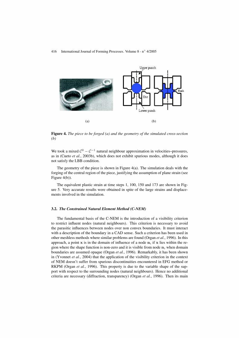
Figure 4. The piece to be forged (a) and the geometry of the simulated cross-section(b)

We took a mixed C0 − C−1 natural neighbour approximation in velocities–pressures,as in (Cueto et al., 2003b), which does not exhibit spurious modes, although it doesnot satisfy the LBB condition.

The geometry of the piece is shown in Figure 4(a). The simulation deals with theforging of the central region of the piece, justifying the assumption of plane strain (seeFigure 4(b)).

The equivalent plastic strain at time steps 1, 100, 150 and 173 are shown in Fig-ure 5. Very accurate results were obtained in spite of the large strains and displace-ments involved in the simulation.

3.2. The Constrained Natural Element Method (C-NEM)

The fundamental basis of the C-NEM is the introduction of a visibility criterionto restrict influent nodes (natural neighbours). This criterion is necessary to avoidthe parasitic influences between nodes over non convex boundaries. It must interactwith a description of the boundary in a CAD sense. Such a criterion has been used inother meshless methods where similar problems are found (Organ et al., 1996). In thisapproach, a point x is in the domain of influence of a node ni if x lies within the re-gion where the shape function is non-zero and it is visible from node ni when domainboundaries are assumed opaque (Organ et al., 1996). Remarkably, it has been shownin (Yvonnet et al., 2004) that the application of the visibility criterion in the contextof NEM doesn’t suffer from spurious discontinuities encountered in EFG method orRKPM (Organ et al., 1996). This property is due to the variable shape of the sup-port with respect to the surrounding nodes (natural neighbours). Hence no additionalcriteria are necessary (diffraction, transparency) (Organ et al., 1996). Then its main


0

0.2

0.4

0.6

0.8

1

1.2

1.4

1.6

1.8

2

0 2 4 6 8 10

−4

−2

0

2

4

6

8

10

121

(a) 1st time step

0

0.5

1

1.5

2

2.5

3

0 2 4 6 8 10

−4

−2

0

2

4

6

8

10

12100

(b) 100th time step

0

1

2

3

4

5

6

7

8

9

10

0 2 4 6 8 10

−4

−2

0

2

4

6

8

10

12150

(c) 150th time step

0

1

2

3

4

5

6

7

8

9

10

0 2 4 6 8 10

−4

−2

0

2

4

6

8

10

12173

(d) 173th time step

Figure 5. Equivalent plastic strain at different time steps of the process

advantages are: no additional computational efforts, and less difficulties to extend themethod for 3D analysis.

We introduce a modified, coined as ’constrained’ Voronoi diagram for non convexdomains. We can view the constrained Voronoi diagram (CVD) or bounded Voronoidiagram as a strict dual to the constrained Delaunay tessellation. The CVD is definedas follows: the intersection of the CVD with the domain closure is composed withcells TCi , one for each node ni, such that any given point x in TCi is closer to ni thanany other node nj visible from point x.

TCi = x ∈ Rn : d(x,ni) < d(x,nj),∀j 6= i,nj visible from ni [15]

The CVD is deduced from the constrained Delaunay tessellation. We introducedthe CVD for the two following reasons: (a) once such diagram is constructed, classical


algorithms for the computation of the shape functions (Braun and Sambridge, 1995)can be applied directly because connections between natural neighbours are removedby the visibility criterion over any non convex domain, and (b) the constrained Voronoicells match precisely integration domains that are used in our integration scheme.

We now define the constrained natural neighbours (C-n-n) like they are first se-lected by the classical natural neighbours criteria (Braun and Sambridge, 1995) (Sukumaret al., 1998) (lying on an empty sphere, sharing one Voronoi cell), and are then re-stricted by the visibility criterion. The trial and test functions result :

uh(x) =

V∑

i=1

φCi (x)ui [16]

where ui are the nodal unknowns, V the number of neighbours nodes visible frompoint x and φCi the constrained natural neighbours shape functions. The C-n-n shapefunctions are similar to NEM shape functions but the support can be different (Yvonnetet al., 2004) and its computation is done on the basis of the CVD.

In Figure 6 we can see that for a point x introduced in the constrained Voronoidiagram, only nodal values from n1, n2 and n3 will contribute to the interpolation,because n4 does not share a constrained Voronoi cell with x. We can conclude that:(a) influences from nodes lying over non convex domains vanish near non convexboundaries because the constrained voronoi diagram removes connexions betweennon mutually visible natural neighbours, and (b) linear interpolation (Sukumar et al.,1998) is satisfied on any boundary (convex or not) by the same considerations.

0 1 2 3 4 5 6 7

3

Γ

Ω

Figure 6. Computation of natural neighbor shape functions over non convex domainby mean of the constrained Voronoi diagram

With this technique, it is trivial to introduce holes, inclusions or discontinuities bysimply adding boundary edges (in 2D) or facets (in 3D) in the boundary description.In (Yvonnet et al., 2004), we have shown that the properties of partition of unity andlinear consistency were met in the crack-tip field neighbourhood with the C-NEMtechnique.


Example: Crack analysis

In order to demonstrate the potential of the C-NEM approach for crack analysis, anumerical example is provided. We examine the case of a centrally located inclinedcrack of length 2a = 0.2 units and an inclination γ in a finite two dimensional squareplate of size 2W × 2W = 2 units, as shown in Figure 7. Plane stress conditions wereassumed with elastic modulus E = 1 MPa and Poisson’s ratio ν = 0.3. A constantload of σ∞22 on both lower and upper sides of the square is applied. We first considerthe case where γ = 0.

γ

2a

y

x

x1θ

σ22

σ22

Figure 7. Modelisation of the plate with an interior inclined crack

This problem has an analytical solution, called Muskelishvili’s solution. This so-lution involves an infinite plate that can not be represented by meshless discretisation.Nevertheless, if the dimension of the crack is small compared with the size of the do-main, the assumption is reasonable. In this example, we took W = 10a. For γ = 0,θ = 0, the exact solution is given by :

σ22(θ = 0, γ = 0) = σ∞22a+r√r(2a+r) [17]

σ11(θ = 0, γ = 0) = σ∞22 − σ22 [18]

No symmetry is considered in the nodal distribution. Numerical results are de-picted in Figure 8. Now, we consider the case of an inclined crack. The stress intensityfactor (SIF) KI is computed using the interaction integral method, and compared inFigure 9 with the analytical solution (Lemaitre and Chaboche, 1990):

KI = σ∞22√πacos2γ [19]


0 0.1 0.2 0.3 0.4 0.5 0.6 0.7 0.8 0.9 10

0.5

1

1.5

2

2.5

3

3.5

4

4.5

5

r/a

Stresses

σ22 σ22 σ11 σ11

Figure 8. Radial stresses ahead of the crack tip for γ = 0

0

0.2

0.4

0.6

0.8

1

σ πα

0 π/4 π/2γ

Figure 9. Normalized stress intensity factor KI for different values of γ

Distance between the nodes near the crack tip is about 0.1a. It can be noticed fromFigs. 8 and 9 that despite of this coarse nodal discretisation, C-NEM solution is in rea-sonable agreement with the analytical solution. Accuracy can be improved by addingnodes in the tip neighbourhood or by enriching shape functions in the framework ofthe partition of unity method (Babuška and Melenk, 1996).

4. An Enriched Assumed Strain Method

Recently, much attention has been focused on a class of finite element methods thatallow for the representation of strong intra-element discontinuities. Among the morenotable are the enhanced assumed strain approaches (Armero and Garikipati, 1996)


(Steinmann et al., 1997), wherein the discontinuous mode is introduced through an en-hanced deformation gradient approximation. In what follows, we provide a summaryof a new formulation presented in (Dolbow and Devan, 2003) that incorporates theintra-element discontinuities directly at the approximation level using an enrichmentstrategy based upon the partition-of-unity framework (Melenk and Babuška, 1996).The new method retains the enhancement to the assumed strain field, as it providesfor coarse-mesh accuracy as well as a means to address volumetric incompressibilityconstraints. We propose a modification to the enhanced strain basis that allows it tobe orthogonal to a piecewise-constant stress field in “cut” elements. The goal is toobtain a robust method for high-speed machining, for example, where large deforma-tions and the isochoric nature of plastic flow place severe demands on the simulationtechnology.

We consider the body identified with a bounded region R of three-dimensionalEuclidean point space <3 that it occupies in a fixed reference configuration. Welabel particles in this reference configuration by X ∈ R with coordinates X =(X1, . . . , Xndim). The deformation ϕ is assumed to satisfy Dirichlet boundary con-ditions ϕ = ϕ on ∂uR ⊂ ∂R. Since we neglect inertial forces, the deformationalforce system consists of the bulk stress P , and imposed tractions T on ∂tR ⊂ ∂R.We allow bulk fields to be discontinuous across the smooth material surface S. In thepresent study, we will assume the surface S to be traction-free.

The variational formulation we employ follows from a three-field Hu-Washizufunctional in ϕ,P , F . Here, F denotes an additional enhanced field to the defor-mation gradient. Precisely, the deformation gradient takes the assumed form

F = GRADϕ+ F , [20]

where GRAD is the gradient operator in the reference configuration.

We let V denote the space of sufficiently regular motions, L the space of suffi-ciently regular stresses and enhanced deformation gradients. The variational boundaryvalue problem is then : Find (ϕ,P , F ) ∈ V × L × L such that

∫

R

2F∂W (C)

∂C· GRAD δϕ dV =

∫

∂tR

T · δϕ dV,

∫

R

(

2F∂W (C)

∂C− P

)

· δF dV = 0, [21]

∫

R

F · δP dV = 0,

for all arbitrary variations (δϕ, δP , δF ) ∈ V × L × L. In the above equations, Wis the bulk strain-energy density function and C is the right Cauchy-Green tensor,C = F TF .


For the sake of concreteness, we consider a standard finite element mesh of four-node quadrilateral elements with nodal shape functions φi. The approximation to thedeformation field is written as

ϕh(X) =∑

i∈I

aiφi(X) +∑

j∈J

bjφj(X)Hd(X), [22]

where I denotes the set of all nodes in the mesh and J the subset that are enriched withthe Heaviside function Hd. The vectors ai and bj are constant degrees of freedom.

Considering a closed subset Ω ⊂ R that is partitioned into complementary subregionsω+ and ω− by the discontinuity S, the Heaviside function is given by

Hd(X) =

1 forX ∈ ω+

0 forX ∈ ω− [23]

The set J of nodes enriched with this function is determined from the “interaction”between the set of overlapping subdomains ωi defining the support of each nodalshape function and the geometry S (Moës et al., 1999) (Dolbow et al., 2000). Since wedo not incorporate asymptotic near-tip functions into the approximation, the presentwork is slightly restricted by the need for the discontinuity to terminate on an elementboundary.

On each elementRe, we consider approximations for F h of the form

F h(ξ) = GRADϕh∣

∣

∣

Re

+∑

i∈E

αi ⊗Gi(ξ), [24]

where E denotes the set of enhancement functions on the element. In the above, Gi

denotes the vector-valued local enhancement functions written in terms of the parentcoordinates ξ, with αi the corresponding degrees of freedom.

In the spirit of earlier efforts (Simo and Armero, 1992), we construct functionsGi that are orthogonal to a subset of the fields spanned by the gradient of [22]. Inparticular, for those elements intersected by S, we seek to construct vector-valuedfunctions Gi that satisfy

∫

¤+

Gi(ξ) d¤ = 0,

∫

¤−

Gi(ξ) d¤ = 0. [25]

where ¤+ and ¤− denote the complementary subsets of the parent domain formedby the intersection of ¤ and the image of S. These functions are then mapped to thereference domain with a constant Jacobian matrix (Simo and Armero, 1992). As such,the functions Gi are orthogonal to piecewise-constant stress fields in “cut” elements,enabling the formulation to satisfy a discontinuous version of the patch test (Dolbowand Devan, 2003). This is in marked contrast to the work of (Armero and Garikipati,1996), where the discontinuous mode was constructed to be orthogonal to a constantstress field only.


We begin with functions Gi that are shifted and linear in ξ. For example, in ¤+,we use

G1(ξ) =

[

ξ1 − ξ1+

0

]

, G2(ξ) =

[

0

ξ2 − ξ2+

]

,G3(ξ) = G4(ξ) = 0. [26]

The shift points, ξ+ in ¤+ and ξ− in ¤−, are determined such that [25] is satisfiedduring numerical integration. An analogous construction is employed on ¤−, withG3 and G4 non-zero. For elements not intersected by S, only the first two functionsabove are employed and the formulation reverts to that proposed in (Simo and Armero,1992).

Substituting the approximations for the deformation and the enhanced gradientinto the Galerkin form of [21] gives rise to a nonlinear system of algebraic equa-tions. This system is resolved using Newton-Raphson iteration to obtain the degreesof freedom ai, bj , and αi. The process is identical to that described in (Simo andArmero, 1992), with the exception of the modified integration schemes employed inthe enriched elements.

A fractured Cook’s membrane problem

We consider finite deformation elastic problems wherein the response is governedby a nearly incompressible neo-Hookean material model. In particular, we employ astored energy function of the form

W =µ

2[J−2/3 tr[C]− 3] +

κ

2(J − 1)

2, [27]

with shear modulus µ and bulk modulus κ. In order to examine the nearly incom-pressible limit, we select κ/µ ≈ 104.

We consider a tapered, fractured panel clamped on one end and subjected to ashearing load on the other as shown in Figure 10. Without the discontinuity, thisproblem is often referred to as ‘Cook’s membrane problem’.

To evaluate the accuracy of the modified enriched/enhanced formulation for theproblem with a discontinuity, we compare our results to those obtained when the crackis explicitly meshed. The enriched and explicitly meshed discretizations are shown inFigures 2a and 2b, respectively. When the crack is meshed, no modification to thestandard assumed strain functions are necessary as the discontinuity is represented bythe doubled nodes along S.

We perform calculations using 30 load steps with increments of ∆F = 1.0N. In allcalculations, we observe an asymptotic quadratic rate of convergence in the Euclideannorm of the residual. The deformed meshes are compared in Figure 10c, and we notethe large deformation and close match of the results. Both approximations satisfythe volumetric constraint reasonably well, with the maximum in |detF − 1| typicallyoccurring near the crack tip, but less than 5%. We conclude that the modified assumedstrain method does not exhibit volumetric locking, and furthermore provides a means


a

b

X

Y

0 10 20 30 40 500

10

20

30

40

50

60

c

Figure 10. Meshes employed for the (a) enriched and (b) standard approxima-tions.The heavy solid line denotes the crack location. (c) Overlay of the final deformedmeshes without magnification. All results shown are for the nearly incompressiblecase, using κ/µ = 104

to represent an evolving discontinuity without any remeshing. Finally, we note thatthe assumed strain framework also lends this method coarse-mesh accuracy.

5. Conclusions

We reviewed MLS- and natural neighbor-based meshless methods. The positiveattributes in the latter were the ease of imposing essential boundary conditions, andthe construction of robust approximations at a relatively low cost. It is simpler to con-struct Ck trial spaces using MLS approximants. Errors due to numerical integrationin meshless methods demand attention. Rigorous mathematical analysis of meshlessmethods is required to develop a better understanding of these methods, and to realizetheir full potential. Partition of unity methods are clearly superior when discontinu-ous phenomena, singularities, or small-scale features need to be captured on a coarsemesh. The partition of unity framework is particularly advantageous for 2-d and 3-d


crack growth simulations; meshless methods such as EFG have had limited success in3-d crack modeling (Sukumar et al., 1997).

Acknowledgements

The support of the National Science Foundation grant number DMI-0223611, toDuke University, is gratefully acknowledged. Also, the support of the Spanish Min-istry of Science and Technology, through the project CICYT-DPI2002-01986 is grate-fully acknowledged.

6. References

Armero F. and Garikipati K. “An analysis of strong discontinuities in multiplicative finite strainplasticity and their relation with the numerical simulation of strain localization in solids”.International Journal of Solids and Structures, vol. 33, no 20-22, 1996, p. 2863-2885.

Babuška I. and Melenk J. M. “The partition of unity finite element method: Basic theory andapplications”. Comp. Meth. in Appl. Mech. and Eng. Vol. 4, 1996, p. 289-314.

Belytschko T., Krongauz Y., Organ D., Fleming M. and Krysl P. “Meshless methods: Anoverview and recent developments”. Computer Methods in Applied Mechanics and Engi-neering. Vol. 139, 1998, p. 3-47.

Braun J. and Sambridge M. “A numerical method for solving partial differential equations onhighly irregular evolving grids”. Nature. Vol. 376, 1995, p. 655-660.

Christ N. H., Friedberg R. and Lee T. D. “Weights of links and plaquettes in a random lattice”.Nuclear Physics B. Vol. 210, no 3, 1982, p. 337–346.

Cueto E., Calvo B. and Doblaré M. “Modeling three-dimensional piece-wise homogeneousdomains using the α-shape based Natural Element Method”. International Journal forNumerical Methods in Engineering. Vol. 54, 2002, p. 871-897.

Cueto E., Cegoñino J., Calvo B. and Doblaré M. “On the imposition of essential boundary con-ditions in Natural Neighbour Galerkin methods”. Communications in Numerical Methodsin Engineering. Vol. 19(5), 2003, p. 361-376.

Cueto E., Doblaré M. and Gracia L. “Imposing essential boundary conditions in the Natural Ele-ment Method by means of density-scaled α-shapes”. International Journal for NumericalMethods in Engineering. Vol. 49-4, 2000, p. 519-546.

Cueto E., Sukumar N., Calvo B., Cegoñino J. and Doblaré M. “Overview and recent advancesin Natural Neighbour Galerkin methods”. Archives of Computational Methods in Engi-neering. Vol. 10(4), 2003, p. 307-384.

Dolbow J. An extended finite element method with discontinuous enrichmentfor applied mechanics. Ph. D. Thesis Northwestern University (1999).

.


Dolbow J., Moës N. and Belytschko T. “Discontinuous enrichment in finite elements with apartition of unity method”. Finite Elements in analysis and design. Vol. 36, 2000, p. 235–260.

Dolbow J. E. and Devan J. E. “Enrichment of enhanced assumed strain methods for representingstrong discontinuities”. International Journal for Numerical Methods in Engineering. Inpress. Preprint available at

!"# .

2003.

Duarte C. A. M. and Oden J. T. “An H-p Adaptive Method using Clouds”. Computer Methodsin Applied Mechanics and Engineering. Vol. 139, 1996, p. 237-262.

Edelsbrunner H., Kirkpatrick D. G. and Seidel R. “On the shape of a set of points in the plane”.IEEE Transactions on Information Theory. Vol. IT-29(4), 1983, p. 551-559.

Edelsbrunner H. and Mücke E. “Three dimensional alpha shapes”. ACM Transactions onGraphics. Vol. 13, 1994, p. 43-72.

Lancaster P. and Salkauskas K. “Surfaces generated by moving least squares methods”. Math-ematics of Computation. Vol. 37, 1981, p. 141-158.

Lemaitre J. and Chaboche J.-L. Mechanics of solid materials. Cambridge University Press,1990.

Li S. and Liu W. K. “Meshfree and particle methods and their applications”. Applied MechanicsReview. Vol. 55, no 1, 2002, p. 1-34.

Melenk J. M. and Babuška I. “The partition of unity finite element method: Basic theory andapplications”. Computer Methods in Applied Mechanics and Engineering. Vol. 139, 1996,p. 289-314.

Moës N., Dolbow J. and Belytschko T. “A finite element method for crack growth withoutremeshing”. International Journal for Numerical Methods in Engineering. Vol. 46, 1999,p. 131-150.

Nayroles B., Touzot G. and Villon P. “Generalizing the finite element method: Diffuse approx-imation and diffuse elements”. Computational Mechanics. Vol. 10, 1992, p. 307-318.

Organ D., Fleming M., Terry T. and Belytschko T. “Continuous meshless approximations fornonconvex bodies by difraction and transparency”. Computational Mechanics. Vol. 18,1996, p. 1-11.

Sethian J. A. “Fast marching methods”. SIAM Review. Vol. 41, no 2, 1999, p. 199-235.

Sibson R. “A Vector Identity for the Dirichlet Tesselation”. Mathematical Proceedings of theCambridge Philosophical Society Vol. 87, 1980, p. 151-155.

Sibson R. “A brief description of natural neighbour interpolation”. In Interpreting MultivariateData. V. Barnett (Editor) 21–36. John Wiley (1981).

Simo J. C. and Armero F. “Geometrically non-linear enhanced strain mixed methods and themetod of incompatible modes”. International Journal Numerical methods in Engineering.Vol. 46, 1992, p. 131-150.


Steinmann P., Larsson R. and Runessson K. “On the localization properties of multiplicativehyperelasto-plastic continua with strong discontinuities”. International Journal of Solidsand Structures. Vol. 34(8), 1997, p. 969-990.

Sukumar N. The Natural Element Method in Solid Mechanics. Ph. D. Thesis NorthwesternUniversity Evanston, Illinois (1998).

Sukumar N., Chopp D. L., Moës N. and Belytschko T. “Modeling Holes and Inclusions by LevelSets in the Extended Finite Element Method”. Computer Methods in Applied Mechanicsand Engineering. Vol. 190(46-47), 2001, p. 6183-6200.

Sukumar N., Moran B. and Belytschko T. “The Natural Element Method in Solid Mechanics”.International Journal for Numerical Methods in Engineering. Vol. 43(5), 1998, p. 839-887.

Sukumar N., Moran B., Black T. and Belytschko T. “An element-free Galerkin method for three-dimensional fracture mechanics”. Computational Mechanics. Vol. 20, 1997, p. 170-175.

Wagner G. J. and Liu W. K. “Hierarchical enrichment for bridging scales and mesh-free bound-ary conditions”. International Journal for Numerical Methods in Engineering. Vol. 50,no 3, 2001, p. 507-524.

Yvonnet J., Ryckelynck D., Lorong P. and Chinesta F. “A new extension of the Natural Elementmethod for non-convex and discontnuous problems: the Constrained Natural Elementmethod”. International Journal for Numerical Methods in Enginering. Vol. 60, 2004,p. 1451-1474.

Received: May 13th 2004

meshless methods and partition of unity finite...

Documents