PATENT HEIGHT AND COMPETITION IN PRODUCT IMPROVEMENTS

by

Theon van Dijk

MERIT Research Memorandum 2/94-015

MERIT Research Memoranda can be ordered from the address below, or be obtained in

electronic form (Postscript) by anonymous ftp at meritbbs.rulimburg.nl

Revised Version, April 1994

ABSTRACT

The stringency of novelty requirements that patent offices and courts use in judging

infringement issues and patentability of inventions defines the height of protection provided

to a patentholder. In this paper the effects of patent height are studied in a duopoly where

firms compete in product improvements. Minimal steps of improvements, determined by the

height, limit the strategy space of competitors who want to invent around a patent. It is

shown that low patents do not affect the natural market equilibrium. A patentholder can lose

with medium patent heights, but he becomes a pure monopolist if patents are high. The non-

patentholder can gain with medium heights but is increasingly worse off with higher patents.

(JEL Code L19, L43, O34)

* This research was sponsored by the Foundation for the Promotion of Research in EconomicSciences, which is part of the Netherlands Organization for Scientific Research (NWO). Ithank, without implicating, Patrick Van Cayseele, Claude Crampes, Paul David, DanielDeneffe, Reinoud Joosten, Eric de Laat and Luc Soete and two anonymous referees forhelpful comments.

Maastricht Economic Research Institute on Innovation and TechnologyUniversity of Limburg, P.O. Box 616, NL-6200 MD Maastricht, The Netherlands

tel (31) (0)43 883869, fax (31) (0)43 216518, Email Merit.Frontdoor@Merit.Rulimburg.nl

1. Introduction

Empirical studies on the appropriability of inventions (e.g., Mansfield et al. (1981), Levin et

al. (1987), Griliches (1990)) provide evidence that patent protection is limited. Many

opportunities are left open for competitors to invent around patents. One can therefore

hardly claim, as is commonly done, that patents provide pure monopoly power. They restrict

at most the opportunities for inventing around. The legal profession is far more aware of this

fact.1 Lawyers are often confronted with the imperfectness of patent protection as the

considerable amount of case law from patent disputes demonstrates (e.g. Cornish (1989) as

a leading textbook on intellectual property).

Until recently, theoretical economists have hardly taken into account the economic and legal

practice of patent protection. Nordhaus’ (1969) seminal work on patent length, for example,

assumes perfect protection during the lifetime of the patent. The same assumption is also

implicitly present in most models of technological competition where the first firm that

generates an invention gets a patent and takes all the profits, leaving the loser of the race no

chances whatsoever (for an overview of patent races, see Reinganum (1989). Recent

contributions aim at relaxing the assumption of perfect protection (Gilbert and Shapiro (1990),

Klemperer (1990)). These studies allow for imitations beside the patent, provided that these

imitations are not too similar. When substitutes in the form of imitations are less similar to

the patented product, the monopoly power of a patentholder increases. Gilbert and Shapiro

are therefore able to define the breadth of patent protection rather generally as the ability of

the patentholder to raise price. Their focus is on the socially optimal mixture between patent

length and breadth. Klemperer defines patent breadth more explicitly within a model of

horizontal product differentiation, as an interval where no competitors are allowed. The

usage of a model of horizontal differentiation turns out to yield richer conclusions about the

optimal mixture, reproducing and extending those of Gilbert and Shapiro.

In this paper, I focus on the height of patent protection. Patent height is mainly determined

by the stringency of the novelty requirements used by examiners in the patent office. Most

patent laws dictate that an invention is only patentable if it is non-obvious and involves an

inventive step. These conditions are certainly satisfied for the small group of fundamental

1 Cornish (1989, p.18) even states: "To the extent that intellectual property is capable of generatingmarket power, it offers its owner (and his associates) the opportunity to reduce output and raiseprices. What it does not bring about is the condition in which the monopolist behaves as though hewere the only competitor on the market. Yet the more naive arguments in favour of one or otherexclusive right often imply that this alone will be the effect of according the right sought."

2

inventions. But the judgement on patentability is more difficult when improvements of

existing products are concerned. When is an improvement obvious and how much

inventivity is required? It is the task of patent examiners to define the bounds of patentability

and infringement of current patents. The central question in this paper is how the height of

patent protection affects the competition in product improvements in a duopoly where one

firm holds a patent, which restricts the strategy set of the other.

Before stressing why the distinction between patent height and breadth is important, let me

first explain the difference. Whereas breadth is defined as the extent of protection against

imitations, height indicates the protection against improvements. In terms of product

characteristics, one could say that height defines the minimal number of new elements which

an invention must contain, whereas breadth defines the maximum number of elements which

are allowed to be imitated. Suppose a patented product is made up of v elements. Think, for

example, of technical attributes like materials, design, electronics schemes, etc., which define

the invention in a unique way. Protection height then indicates how many new elements h

are required in order not to infringe an ongoing patent. Breadth defines the maximum

number b out of the v that is allowed to be imitated without infringing.

The difference between imitations and improvements can be found on both the cost side and

the demand side. Although imitations may also require investment in R&D in order to obtain

learning and imitation capabilities (Cohen and Levinthal (1989)), improvements are likely to

cost more R&D because new information has to be generated. With regard to the demand

side, as previously explained, Klemperer (1990) treats imitations as horizontal differentiations

of the patented product. Consumers do not agree on the most preferred variety. Some

consumers prefer protected varieties, while others prefer imitations outside the protected

interval. Improvements are basically different from imitations in this respect. Improvements

can be considered as vertical differentiations. It is reasonable to expect that, at equal prices,

all consumers prefer an improvement to an older version of the product. Patent height can

then be thought of as defining a protected region on the vertical product spectrum.

Competitors that enter the market are restricted in their choices of improvement. They must

generate a minimum level of improvement in order not to infringe the current patent.2 The

dimensions of breadth and height thus define protection against two different types of

competition; one resulting from horizontal differentiation and another resulting from vertical

differentiation. These two types of competition have a differential impact on the patentholder.

2 The literature on minimum quality standards also uses vertical differentiation models (e.g.,Ronnen (1991) and Crampes and Hollander (1991)). The major difference with the analysis presentedhere is that only the non-patentholder is restricted in my model whereas in the other modelsmentioned both firms are restricted.

3

The effect of vertical differentiation is that it relaxes price competition; therefore firms have

a tendency to differentiate their products maximally (Shaked and Sutton (1982)). Horizontal

differentiation may have an opposite effect. At least for linear transport costs, as in the

original Hotelling (1929) analysis, firms differentiate minimally.

Taking these cost and demand features into account, two basic strategies for inventing

around a patent can be distinguished: an imitation strategy "aside" the patented product and

an improvement strategy "above" it. An example may clarify the two possible strategies.

Klemperer (1990, p. 114) mentions the patent of Prince Manufacturing on the oversized tennis

racket. The breadth of protection is known to run from 85 to 130 square inches rackets. A

competitor pursuing an imitation strategy can only enter with a similar racket outside this

protected range. But there is also another possibility, not examined by Klemperer. A

competitor can improve a racket inside the range in such a way that it satisfies patent

examiners. For example, a 100 square inches racket can be made stiffer by the use of a new

fibre or a better design. Both cost and demand properties can play an important role in

choosing the appropriate inventing-around strategy. An imitation strategy has a relative cost

advantage but may be more severely restricted by patent breadth because, being a horizontal

differentiation, the imitation may be chosen close to the patented product. A competitor that

pursues an improvement strategy has a natural tendency to create distance away from the

patent, but this tendency may be suppressed by high R&D costs. The impact of the imitation

strategy on the patentholder’s profits has been examined in the above mentioned models of

patent breadth. So far, however, the impact of the improvement strategy has not been

analyzed.

This paper will concentrate on the effects of novelty requirements once a patent is granted.

Scotchmer and Green (1990) have analyzed a related problem. They discuss the social trade-

off that occurs in setting the novelty requirements when firms apply for patents. Novelty

requirements appear to have a dual character. They determine the coverage of granted

patents - the study object of this paper -, but they also affect the stage of R&D competition

before the patent is possibly granted. This second aspect is studied in Scotchmer and Green

(1990). The main benefit of weak novelty requirements then is that technical information

becomes public at an earlier date so that other firms can build further on it sooner. However,

weak requirements may also induce the inventor to withhold his invention, thereby keeping

the lead, and aim at a more profitable invention later on. Strong novelty requirements reduce

the amount of wasteful duplicative R&D by inducing firms that have fallen behind to drop

out of the race. In order to focus fully on the extent of protection, I will omit the stage of

R&D competition here.

4

The plan of this paper is as follows. In section 2, a model is constructed which is based on

the idea of improvements being vertical differentiations of a new product. First, I examine

the competition in product improvements in the absence of patents. In section 3, I will

analyze the effects of patent height on the competition in product improvements. In a

nutshell, the major conclusions are that low patent heights do not affect the natural market

equilibrium without patents, medium heights can be favourable and unfavourable for the

patentholder, and high patents provide pure monopoly power. Conclusions and possible

applications are presented in section 4.

2. The Model

The starting point of the analysis is the appearance of a basic invention. In this section, I

assume that this basic invention is public property. The basic invention is so raw that no

consumer is prepared to buy it. Consumers can only extract surplus from the basic invention

if it is further developed. Defining the demand side more precisely, the net surplus U of an

individual consumer is given by the following (indirect) utility function:

U = mv - p if the consumer buys (1)

0 otherwise

where v ∈ [0, ∞⟩ is the degree of improvement (with the basic invention given by v = 0), p

is the price of improvement v and m is a parameter indicating the intensity with which a

consumer prefers improvements. The parameter m is uniformly distributed with density 1

on [b - 1, b], where 1 < b < 2. A consumer only buys if he gets a non-negative net surplus.

Each consumer decides in each period whether or not to buy (one unit). The utility function

(1) is standard in the literature on vertical differentiation (e.g. Shaked and Sutton (1982)).

Applying function (1) in the context of technical change is justified because consumers are

expected to evaluate product improvements in much the same way as qualities of a product.

Consumers prefer large to small improvements, just like they prefer high to low-quality

products.

There are two firms, 1 and 2, potentially entering the new market with improvements of the

basic invention. Each of the firms is assumed to offer one improvement at the most. There

are two motivations behind this assumption. First, the diversity of consumers’ tastes (given

by the range of m) is chosen such that there is only room at the market for two

improvements. Competition analysis then requires that each of the two firms has one

improvement at the most. Second, it is true that in business practice one can often observe

that a firm does not have one patent but a number of related patents, all in the same

5

technical field. But even such a cluster of patents cannot provide perfect protection.

Competitors can still invent around the cluster. Essentially we are then back at the scenario

studied in this paper: one firm has a patent (or a cluster of patents) and another firm enters

the market with an improvement (of the most advanced patent of the cluster). Once chosen,

I assume that an improvement cannot be changed. As we will see below, there are

circumstances under which it would be beneficial for a firm to lower its improvement level.

However, high fixed costs associated with each improvement are assumed to prevent this.

The competition between both firms takes place in two stages. In the first stage, each firm

decides whether or not to enter the market and which improvement to choose. Knowing

which decisions are made in the first stage, each firm then chooses a price strategy. This

sequence reflects the fact that price decisions are more flexible than improvement and entry

decisions. The solution concept that I employ for this two-stage model is the subgame perfect

equilibrium. It can be obtained by backward induction. First, I will determine the Nash

equilibrium in pricing strategies of the second stage. In the second stage, I will determine the

equilibrium strategies in product improvements and entry. Only pure strategies are

considered.

It is assumed here that both firms are characterized by the same R&D cost structure, which

is kept as simple as possible. There are no development costs involved in the generation of

improvements. It only costs time. Starting at time 0, firm i introduces vi in period Ti, where

Ti = αvi, for i ∈ {1, 2} and 0 ≤ α ≤ 1. The profit that is lost because of a later introduction time

is the real development cost. If both firms enter the market, the first-stage subgame is defined

by a pair of improvements {vS, vL}, such that vS ≤ vL. The subscript S denotes the firm that

has developed an improvement that is smaller than the other improvement. The other firm

has the larger improvement and is denoted by subscript L. Note that each firm can develop

either the small improvement or the large improvement. Assuming that both firms start their

development in the same period, vL is always introduced later than vS. As a consequence, the

market structure can change over time. The firm with vS will enter in period TS. It then has

a temporary monopoly position and sets a monopoly price, denoted by pM. This monopoly

will last until the other firm enters at TL with vL. From TL until a doomsday J the market

structure then will be a duopoly. By assumption, the former monopolist can only react to the

entrant by setting a new price, denoted by pS, as a function of the entrant’s price pL.

Assuming that all consumers are price and improvement takers, during monopoly each

consumer has the choice between buying vS at price pM or not buying at all. Consumer

choices extend when the later firm introduces vL at TL. Each consumer can then choose to buy

vS at price pS, vL at price pL, or none of the improvements.

6

2.1. Price Competition

The following demand function is relevant in two cases. First, in the scenario in which only

one firm enters the market and remains a monopolist until doomsday J. Second, during the

period when the small improvement firm is alone in the market and the other firm has not

entered yet.

D(pM) = b - pM/vS (2)

for pM/vS > b - 1. Without affecting the basic results, I assume that the unit production costs

are zero. It can be shown that the monopoly price and profit per period are pM* = bvS/2 and

πS(pM*) = b2vS/4. The lower market segment [b - 1, b/2] is not served.

Now consider the demand functions in case of duopoly. The consumer who is indifferent

during duopoly as to the small and large improvement is given by the preference parameter

µ = (pL - pS)/(vL - vS). The firm with vS, which charged pM before, now changes its price and

charges pS. For computational ease, I assume that the market is served completely during

duopoly. I take (vS + 2vL)/(2vS + vL) < b < 2.3 The demand functions are then:

DS(pS; pL) = µ + 1 - b, DL(pL; pS) = b - µ (3)

The Nash equilibrium prices are pSN = (2 - b)(vL - vS)/3 and pL

N = (b + 1)(vL - vS)/3, with

associated profits of πS(pSN; pL

N) = (2 - b)2(vL - vS)/9 and πL(pLN; pS

N) = (b + 1)2(vL - vS)/9 (see

Tirole (1988) for an elaboration).

2.2. Competition in Product Improvements

First, I will examine the pure monopoly scenario, where the monopoly position lasts from

the introduction time until the doomsday J. The monopolist will have profits πS(pM*), as

determined above. The profit function of such a monopolist in the first stage is:

πS(vS) = (J - TS)πS(pM*) (4)

In order to keep the analysis as simple as possible, I assume that pay-offs are not discounted.

A similar effect originates from the doomsday J, when everything ends. The monopolist is

confronted with the following trade-off: on the one hand, his profit per period increases if

he develops a larger improvement, but on the other hand, it costs more development time

3 This condition turns out to be always possible in the analysis to follow. All equilibrium valuesof vS and vL fulfill the condition that 1 < (vS + 2vL)/(2vS + vL) < 2.

7

so that there will be less time to capitalize on his investments. The next step is to calculate

the optimal improvements as a function of each other, given the equilibrium prices

determined above. After substitution of the time cost structure TS = αvS and the optimal

profit πS(pM*) in (4), the optimal improvement of the monopolist can simply be determined

as vS* = J/2α, with the associated optimal profits of πS(vS*) = b2J2/16α. The optimal

improvement vS* increases if the monopolist is given more time (later J) and if the

development costs are lower (smaller α). The optimal monopoly profit πS(vS*) also increases

if the demand properties are more favourable; a higher b means that improvements are more

valued by consumers.

When two firms enter the new market, the profits of the firm with vS contain monopoly

profits, gained from TS until TL, and duopoly profits, from TL until doomsday J:

πS(vS; vL) = (TL - TS)πS(pM*) + (J - TL)πS(pSN) (5)

The profit function of the firm that enters later at TL with vL is:

πL(vS; vL) = (J - TL)πL(pLN) (6)

Before proceeding further, I want to emphasize some important properties of the profit

functions (5) and (6). The profit per period πS(pM*) in equation (5) increases in vS. This

property was already mentioned above in the pure monopoly case. In order to simplify the

notation, let q ≡ b2/4, so that πS(pM*) = qvS. The duopoly profits per period πS(pSN) and πL(pL

N)

decrease in vS for the small improvement firm (5) as well as the large improvement firm (6).

This property is well known in the vertical product differentiation literature and is the result

of more relaxed price competition as products are more differentiated (Shaked and Sutton

(1982)). It can also be found in the way profits behave in vL. Since a larger vL means a larger

distance between both improvements, the profits per period increase for both firms. Define

r ≡ (2 - b)2/9 and s ≡ (b + 1)2/9, so that πS(pSN) = r(vL - vS) and πL(pL

N) = s(vL - vS). For the

values of b which are taken here it holds that s > q > r. This ranking will turn out to be

important further on.

After substitution of the introduction times and the profits in the second stage in the profit

functions (5) and (6), the following improvement reaction functions can be derived:

vS*(vL) = vL(q + r)/2q - rJ/2αq (7a)

vL*(vS) = vS/2 + J/2α (7b)

8

where vS, vL ∈ [0, J/α]. An important property of (7a) is that it implies that πS increases

monotonically in vS along the reaction curve. This can be checked by substituting (7a) into

(5) and taking the first derivative of πS with respect to vS*, which turns out to be positive. The

intuition behind this is the following. If vL increases, vS* also increases, but by less (since (q

+ r)/2q < 1). The number of monopoly periods as well as the monopoly profit per period

increase. The profit per period in duopoly also increases because the distance between vL and

vS becomes larger. These positive effects on πS outweigh the only negative effect of a smaller

number of periods before doomsday. The opposite holds for the firm with the large

improvement; πL decreases monotonically in vL along the reaction curve (7b). The intuition

is simple. Suppose vS increases. As a consequence, vL* will increase but only by half as much,

so that the distance between both improvements becomes smaller. Considering, in addition,

that the remaining time before doomsday shrinks, it is clear that πL decreases.

The Nash equilibrium in the first stage of competition in product improvements can be found

by solving the reaction functions (7a) and (7b) simultaneously for vS and vL. Define this

solution as the basic Nash equilibrium {vSN, vL

N}, given by:

vSN = J(q - r)/α(3q - r)

vLN = J(2q - r)/α(3q - r) (8)

Between TS and TL, the upper segment of the market [b/2, b] is served by the temporary

monopolist with improvement vSN at a price of pM* = bJ(q - r)/2α(3q - r). When the other firm

enters in period TL with the large improvement vLN, it serves more customers than the

monopolist. The upper market segment [(2b - 1)/3, b] is served at a higher price of pLN = ((2b

- a)Jq)/3α(3q - r). The small improvement firm now serves the lower market segment [b - 1,

(2b - 1)/3], which was not served before, at a price of pSN = ((2b - 1)Jq)/3α(3q - r).

In this basic Nash equilibrium, the overall profit of the firm with the small improvement

(πS(vSN)) turns out to be positive and lower than that of the firm with the large improvement

(πL(vLN)): q3J2/α(3q - r)2 < sq2J2/α(3q - r)2, since s > q. It is not clear in advance which firm

will have the large improvement. There are in fact two basic Nash equilibria in pure

strategies. One in which firm 1 has the small improvement and firm 2 has the large

improvement {v1 = vSN, v2 = vL

N} and one where this division of roles is reversed {v1 = vLN,

v2 = vSN}.

9

3. The Effects of Patent Height

This section studies scenarios where the basic invention is privately owned. One of the two

firms, say firm 1, disposes of the basic invention. Two cases are studied: [1] firm 1 cannot

keep the basic invention secret, not even for a very short period of time; and [2] firm 1 can

keep the basic invention perfectly secret. Any level of the first improvement can be protected

by a patent. The patent system under consideration is assumed to be a "first-to-file" patent

system4. The patent protection is of infinite length and of height h.5 It is assumed that the

criterion for judging infringement is precise and known by the patentholder and his

competitor6. The meaning and effects of the patent height h are explained below. It is

furthermore assumed that licensing is not possible. Since I want to focus purely on

competition aspects, all forms of cooperation are excluded. The impact of excluding licensing

will become clear below. To simplify the notation, without affecting the results, I take J = 1

and α = 1 from now on.

3.1 Secrecy is Impossible; Patent on the Basic Invention

In scenario [1], firm 1 is assumed to patent the basic invention immediately (given the lack

of secrecy and the first-to-file rule, firm 2 may do so otherwise). I will come back to this

assumption below. The technical information in the patent application becomes public and

causes both potential entrants to start their development work with the same knowledge

level. Hence, there is no asymmetry as far as knowledge is concerned. However, there is

asymmetry because firm 1 has a patent on the basic invention and firm 2 has not. The patent

is not a barrier to entry that cannot be overcome. It only protects a limited area beyond the

basic invention. More precisely, the protection of the patent with height h is the region [0,

h⟩.7 The non-patentholder is not allowed to choose his improvement in this region. He has

4 In cases of dispute when two firms claim the same patent, the first-to-file rule says that the firmthat filed the application first possibly obtains it. This rule applies in all countries except the US, whichapplies the "first-to-invent" rule.

5 Since competitors are assumed to choose an improvement and not an imitation of the patentednew product, the breadth of protection is not important here. Case law seems to indicate that thenovelty requirements overrule the allowed similarity of imitations (Cornish (1989)). In other words,an identical variety, provided that it is improved sufficiently, is permitted. Mixtures of patent breadthand height as well as optimal strategies for inventing around are studied in Van Dijk (1993).

6 Waterson (1990) examines a patent system where it is not clear beforehand whether thepatentholder or the possible infringer wins in court. This uncertainty may affect the patenting decision.

7 In their judgement on non-obviousness and inventivity, patent examiners mainly rely on files offormer patent applications. The body of knowledge in these files represents to a large extent the(accessible) state of the art, which serves as a benchmark for examination. This is the reason why theprotection starts from 0, i.e. the patented basic invention.

10

to choose his improvement in the free, not protected region [h, 1].

The second stage of price competition is not affected by the institution of patent heights. The

first stage of competition in product improvements, however, can yield different results. Both

firms keep on choosing their improvements simultaneously. The strategy space of the non-

patentholder 2 shrinks to v2 ∈ [h, 1]. The strategy space of firm 1 remains unchanged v1 ∈[0, 1]. This asymmetric effect of patent height is the major difference with the models on

minimum quality standards of Ronnen (1991) and Crampes and Hollander (1991). In their

models, the minimum standard symmetrically limits the strategy spaces of both firms. With

firm 1 holding a patent, each of the firms can still choose the small or large improvement in

equilibrium. But we will see that, depending on the height of protection, the improvements

can become larger compared to those in the basic Nash equilibria. We will also see that in

one category of heights, one basic Nash equilibrium will not occur.

The effects of patent height can be divided into five categories. The two categories for

extreme values of h are obvious. Low patents (0 ≤ h ≤ vSN) do not affect the basic Nash

equilibria. Firm 2 can still have the small improvement without being restricted effectively.

In the other extreme category of high patents (h ≥ 1), firm 2 does not have enough time to

develop an improvement that does not infringe the patent of firm 1. The patentholder is then

assured to have a monopoly position until doomsday 1 and the only improvement that will

be on the market is v1 = 1/2. For the medium values vSN < h < 1, three categories can be

distinguished (see Propositions 1.a. and 1.b.). Two categories contain heights for which firm

2 is effectively restricted in the choice of the small improvement (Proposition 1.a.). These

heights turn out to be unfavourable for the patentholder if he has the large improvement,

because firm 1 loses profit compared to the basic Nash equilibrium. For firm 2, the non-

patentholder, these patent heights are initially favourable.

Proposition 1.a. For h ∈ ⟨vSN, h⟩ there are two Nash equilibria in pure strategies (h will be

defined below): a basic Nash equilibrium with v1 = vSN and v2 = vL

N and a new Nash

equilibrium with v2 = h en v1 = vL*(h). In the new Nash equilibrium (a) both improvements

are larger than in the comparable basic Nash equilibrium; (b) the profit of the patentholder

1 decreases in h; and (c) the profit of the non-patentholder initially increases and later

decreases in h. For h ∈ [h, vLN], the only basic Nash equilibrium is v1 = vS

N en v2 = vLN.

Firm 2 is effectively restricted in the choice of the small improvement and not in the choice

of the large improvement for the heights vSN < h ≤ vL

N. What are the consequences? The one

basic Nash equilibrium in which firm 1 has the small and firm 2 has the large improvement

remains unchanged. The other basic Nash equilibrium, however, is no longer possible

11

because firm 2 is not allowed to enter the market with the improvement vSN. The smallest

improvement permitted to firm 2 is exactly equal to the height v2 = h.8 Firm 1 will react

according to (7b) with an improvement v1 = vL*(h). Note that both improvements h and vL*(h)

are larger than in the relevant basic Nash equilibrium with v2 = vSN and v1 = vL

N; h > vSN

holds by definition, and vL*(h) > vLN because ∂vL*/∂vS > 0.

The optimal profit of the large improvement firm decreases in vL along its reaction curve, as

has already been shown in section 2.2.. Hence, if firm 1 has the large improvement, its profit

πL decreases in h for h ∈ ⟨vSN, vL

N]. This can be seen in figure 1, where π1’ represents a lower

profit level than π1. Since the firm with the large improvement has the higher profits in basic

Nash equilibrium and these profits now decrease in h for the patentholder, there must be a

value for h where the patentholder collects the same profits with the large improvement as

with the small improvement, with firm 2 choosing vS = h. Label this critical value for firm

1 as h, defined as πL(h, vL*(h)) = πS(vSN, vL

N). For h > h, the patentholder prefers to have the

small improvement instead of the large one.

v (v )

v (v )

1 2

2 1*

*

v 2v2

Nh

v

v (h)1

1N

*

v1

0

π

π 2

2

’π

π

1

1’

’

Figure 1. Patent on the Basic Invention; Firm 2 has the Small Improvement

8 I restrict the analysis to one patent. I assumed that an improver cannot get a patent. Allowing fora second patent complicates matters since the basic inventor has to take into account that his strategyspace might also be restricted if the improver has a patent.

12

What happens to the profits of firm 2 when it has the small improvement? For h < h, firm

2 has to deviate from its reaction function (7a) and has to choose the small improvement

larger than in the basic Nash equilibrium. As a result its profits will initially increase in h.

Profits will increase up to the height h’, where h’ is equal to the product improvement that

firm 2 would choose it were Stackelberg leader. In figure 1, π2’ represents the (Stackelberg)

profit level of firm 2 given patent height h’. This profit level is higher than the one in the

basic Nash equilibrium, π2. Profits start decreasing for firm 2 from h’ on.9 For h > h, the

patentholder does not even want the large improvement anymore and leaves it to the non-

patentholder, despite the fact that it yielded more profits in the basic Nash equilibrium. The

economic intuition behind this surprising result is that patent height forms a credible

commitment which the non-patentholder can exploit. Initially the non-patentholder is

credibly committed to choosing a larger vS than in basic Nash equilibrium. For even higher

patents (h > h), the commitment becomes so strong that the non-patentholder always has the

more profitable large improvement10.

9 I limit the analysis here to the case where h > h’. The maximum profits of firm 2 in the turningpoint do not exceed the profits with the large improvement in the basic Nash equilibrium. In the caseof h < h’, firm 2’s profit only increases in h for h ∈ ⟨vS

N, h⟩. If the maximum profit in the turning pointh’ is larger than the profit associated with the large improvement in the basic Nash equilibrium, thenan extra category can be distinguished in which firm 2 prefers the small improvement h and firm 1prefers the large improvement vL*(h).

10 This disadvantage for the patentholder may depend on two assumptions made above. First, theassumption that firm 1 patents immediately may be important here because, without the patent, thepossibility would stay open for firm 1 to have the more profitable large improvement. As we will seebelow, however, from a critical protection on it is beneficial again for firm 1 to have the patent. Bywaiting and patenting later, the protection associated with an improvement patent becomes larger (vL

≥ vS + h). But firm 2 could then obtain the patent as well. A critical height must exist for which bothfirms are indifferent to having the patent or not. It could well be the case that the profits, associatedwith this critical height, are lower than the profits of the firm with the small improvement in the basicNash equilibrium (e.g., if the profits associated with the restricted large improvement are lower thanthose associated with the patented small improvement and there is some probablility of not obtainingthe patent). For these cases, firm 1 would patent immediately anyway.

Another way out of the disadvantageous patent position might be licensing. Althoughlicensing is excluded from the present analysis, I will comment on it briefly here. Note that thepatentholder has an incentive to offer, even freely, the improver a license, allowing him to choose animprovement inside the protected region. Profits of the patentholder would increase. The profits ofthe improver and license taker would, however, decrease. Thus, unless the patentholder is able toprecommit to license its patent freely, a license contract would not emerge. And even if suchprecommitment is possible (e.g., if the patent office recognizes the one-sided free gift and adjusts itsstandards of examination, or if licensing is compulsory), the improver may be able to precommit notto accept the free gift (e.g., by provoking a court or patent office judgement). If the patentholder canprecommit to license freely and the improver cannot precommit not to accept, the basic Nashequilibrium where the patentholder has the large improvement would reoccur.

13

This advantage for the improver, however, disappears. From a certain height on, the

commitment becomes an obligation; firm 2 must choose a larger improvement than it would

like to. Higher patents then yield more profit for the patentholder and less for the non-

patentholder if the latter is also effectively restricted in the choice of the large improvement.

The following proposition holds:

Proposition 1.b. For h ∈ ⟨vLN, 1⟩ there is one Nash equilibrium with v1 = vS*(h) and v2 = h.

The Nash equilibrium is characterized by (a) larger improvements than in the relevant basic

Nash equilibrium; (b) an increasing profit of the patentholder in h; and (c) a decreasing profit

of the non-patentholder in h.

Firm 2 is effectively restricted in its choice of the large product improvement for the patent

heights h ∈ ⟨vLN, 1⟩. The choice of vL

N is not allowed and firm 2 does best choosing h. The

best reaction of the patentholder is vS = vS*(h). The only Nash equilibrium is characterized

by a small improvement of the patentholder of v1 = vS*(h) and a large improvement of firm

2 of v2 = h. Note that both improvements are larger than in the relevant basic Nash

equilibrium; h > vLN holds by definition, and vS*(h) > vS

N because ∂vS*/∂vL > 0. In section 2,

I demonstrated that the optimal profits of the small improvement firm always increase in vS

along the reaction curve (7b). The profits of the patentholder thus increase in h for h ∈ ⟨vLN,

1⟩. What happens to the profits of the non-patentholder? He has to deviate from his reaction

curve. The isoprofit curve that passes through the new Nash equilibrium now represents its

lower profit level11. Hence, the profits of firm 2 decrease in h for h ∈ ⟨vLN, 1⟩. The patent

height has changed for firm 2 from a profitable commitment into a profit-loosing obligation.

The five categories are summarized in table 1 with the values that follow from the used

specification.

11 It is possible that firm 2 does not enter the market for h < 1. This is the case from that heightwhere the isoprofit curve in the new Nash equilibrium also cuts the 45 line with vS = vL. The profitof the entrant is zero if both product improvements are identical; it is well known that Bertrandcompetition with homogeneous products leads to zero profits. When lower than 1, this critical patentheight is the upper limit.

14

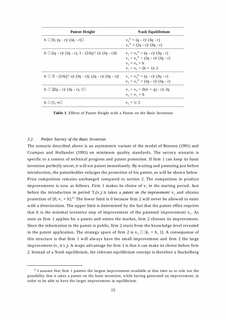
Patent Height Nash Equilibrium

h ∈ [0, (q - r)/(3q - r)⟩ vSN = (q - r)/(3q - r)

vLN = (2q - r)/(3q - r)

h ∈ [(q - r)/(3q - r), 1 - (2√(q3/s)/(3q - r))] v1 = vSN = (q - r)/(3q - r)

v2 = vLN = (2q - r)/(3q - r)

v2 = vS = hv1 = vL = (h + 1)/2

h ∈ ⟨1 - (2√(q3/s)/(3q - r)), (2q - r)/(3q - r)] v1 = vSN = (q - r)/(3q - r)

v2 = vLN = (2q - r)/(3q - r)

h ∈ ⟨(2q - r)/(3q - r), 1⟩ v1 = vS = (h(r + q) - r)/2qv2 = vL = h

h ∈ [1, ∞⟩ v1 = 1/2

Table 1. Effects of Patent Height with a Patent on the Basic Invention

3.2. Perfect Secrecy of the Basic Invention

The scenario described above is an asymmetric variant of the model of Ronnen (1991) and

Crampes and Hollander (1991) on minimum quality standards. The secrecy scenario is

specific to a context of technical progress and patent protection. If firm 1 can keep its basic

invention perfectly secret, it will not patent immediately. By waiting and patenting just before

introduction, the patentholder enlarges the protection of his patent, as will be shown below.

Price competition remains unchanged compared to section 2. The competition in product

improvements is now as follows. Firm 1 makes its choice of v1 in the starting period. Just

before the introduction in period T1(v1) it takes a patent on the improvement v1 and obtains

protection of [0, v1 + h].12 The lower limit is 0 because firm 2 will never be allowed to enter

with a deterioration. The upper limit is determined by the fact that the patent office requires

that h is the minimal inventive step of improvement of the patented improvement v1. As

soon as firm 1 applies for a patent and enters the market, firm 2 chooses its improvement.

Since the information in the patent is public, firm 2 starts from the knowledge level revealed

in the patent application. The strategy space of firm 2 is v2 ∈ ⟨v1 + h, 1]. A consequense of

this structure is that firm 1 will always have the small improvement and firm 2 the large

improvement (v1 ≤ v2). A major advantage for firm 1 is that it can make its choice before firm

2. Instead of a Nash equilibrium, the relevant equilibrium concept is therefore a Stackelberg

12 I assume that firm 1 patents the largest improvement available at that time as to rule out thepossibility that it takes a patent on the basic invention, while having generated an improvement, inorder to be able to have the larger improvement in equilibrium.

15

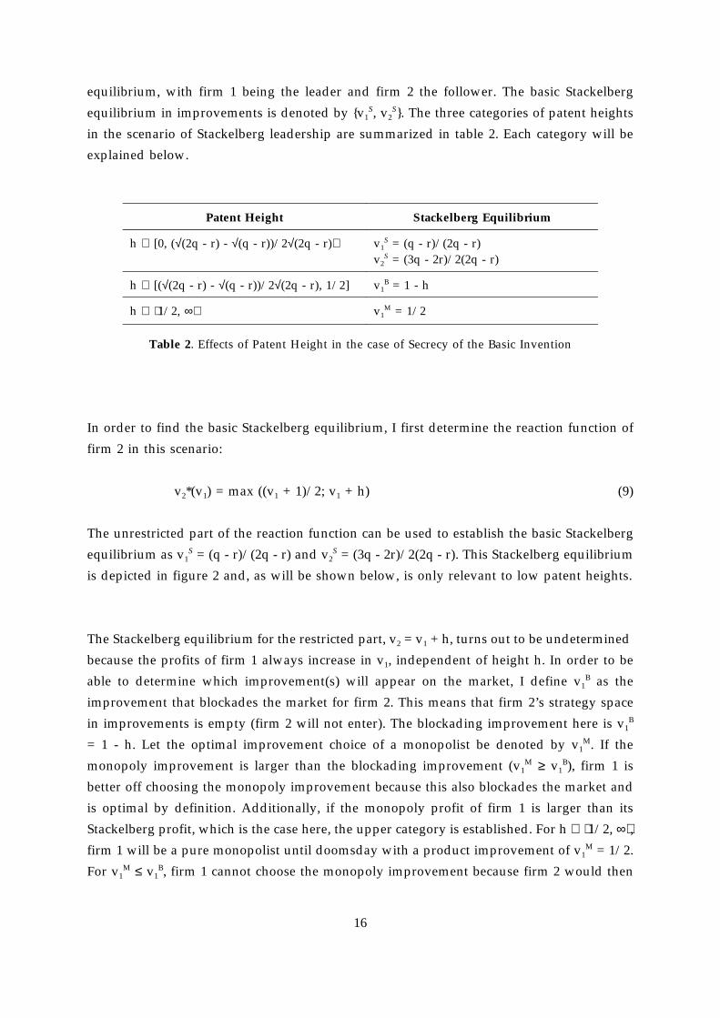
equilibrium, with firm 1 being the leader and firm 2 the follower. The basic Stackelberg

equilibrium in improvements is denoted by {v1S, v2

S}. The three categories of patent heights

in the scenario of Stackelberg leadership are summarized in table 2. Each category will be

explained below.

Patent Height Stackelberg Equilibrium

h ∈ [0, (√(2q - r) - √(q - r))/2√(2q - r)⟩ v1S = (q - r)/(2q - r)

v2S = (3q - 2r)/2(2q - r)

h ∈ [(√(2q - r) - √(q - r))/2√(2q - r), 1/2] v1B = 1 - h

h ∈ ⟨1/2, ∞⟩ v1M = 1/2

Table 2. Effects of Patent Height in the case of Secrecy of the Basic Invention

In order to find the basic Stackelberg equilibrium, I first determine the reaction function of

firm 2 in this scenario:

v2*(v1) = max ((v1 + 1)/2; v1 + h) (9)

The unrestricted part of the reaction function can be used to establish the basic Stackelberg

equilibrium as v1S = (q - r)/(2q - r) and v2

S = (3q - 2r)/2(2q - r). This Stackelberg equilibrium

is depicted in figure 2 and, as will be shown below, is only relevant to low patent heights.

The Stackelberg equilibrium for the restricted part, v2 = v1 + h, turns out to be undetermined

because the profits of firm 1 always increase in v1, independent of height h. In order to be

able to determine which improvement(s) will appear on the market, I define v1B as the

improvement that blockades the market for firm 2. This means that firm 2’s strategy space

in improvements is empty (firm 2 will not enter). The blockading improvement here is v1B

= 1 - h. Let the optimal improvement choice of a monopolist be denoted by v1M. If the

monopoly improvement is larger than the blockading improvement (v1M ≥ v1

B), firm 1 is

better off choosing the monopoly improvement because this also blockades the market and

is optimal by definition. Additionally, if the monopoly profit of firm 1 is larger than its

Stackelberg profit, which is the case here, the upper category is established. For h ∈ ⟨1/2, ∞⟩,firm 1 will be a pure monopolist until doomsday with a product improvement of v1

M = 1/2.

For v1M ≤ v1

B, firm 1 cannot choose the monopoly improvement because firm 2 would then

16

enter. Instead, firm 1 chooses the blockading improvement. Compared to the optimal

v (v )

v (v )*

*

v

v1 2

2 1

1

2

2

v1S0

h

v + h1

vS

Figure 2. Patent on the First Improvement

monopoly profits, the blockading profits decrease if v1B is further away from v1

M, i.e., when

patents are lower. The loss in profits due to the strategy of market blockade becomes large

to the extent that, from a critical patent height on, firm 1 is better off being a Stackelberg

leader in duopoly than a blockading monopolist. Label this height as h", defined as π1(1 - h")

≡ π1S(v1

S, v2S). The two remaining categories can now be determined. For h ∈ [h", 1/2], firm

1 will be a blockading monopolist until doomsday with the blockading improvement v1B =

1 - h.13 For h ∈ [0, h"⟩, firm 1 will be Stackelberg leader in duopoly. Proposition 2

summarizes the three categories of patent heights.

Proposition 2. For h ∈ [0, h"⟩ the improvements developed in the Stackelberg equilibrium are

v1S and v2

S. For h ∈ [h", 1/2] the patentholder is a blockading monopolist with an

improvement of v1B = 1 - h; the profits of the patentholder increase in h until monopoly

profits are reached for h = 1/2. The patentholder continues to be a monopolist for h ∈ ⟨1/2,

∞⟩ with an improvement of v1M = 1/2.

13 The critical height h" in the used specification is not larger than the natural distance between thesmall and the large improvement in the basic Stackelberg equilibrium (h" ≤ v2

S - v1S). The third

category, for low patents, then is h ∈ [0, h"⟩. Firm 1 will first come up with v1S. Afterwards, firm 2

follows with v2S.

17

3.3. Patent Height and Welfare

The static welfare in the market can be determined in a simple manner because of the linear

demand structures resulting from utility function (1). The sum of consumer and producer

surplus can be taken as an approximation for the total welfare. A product improvement

generates a level of welfare equal to 3/2 of the total profit, both under monopoly and under

duopoly. Maximization of welfare is thus equivalent to maximization of joint profits. It can

easily be shown that with a patent on the basic invention (scenario [1]), the optimal patent

height from a social point of view is given by h* = (r + s)/(2s - q + r)) inside the category h

∈ ⟨vLN, 1⟩ in which the Nash equilibrium with vS = vS*(h) and vL = h occurs. All heights in

the category [0, h"⟩ where a Stackelberg equilibrium with v1S and v2

S occurs are socially

optimal in scenario [2].

These welfare conclusions are concerned with the static efficiency once the basic invention

is generated. However, a more complete welfare analysis in the context of technical progress

would take into account the necessity of an incentive for research. The presence of a basic

invention as a starting point is appropriate for competition analysis but not for welfare

analysis. How can this research incentive be taken into account? In Klemperer (1990) and

Gilbert en Shapiro (1990), it is introduced in the form of a minimial profit V for the firm that

undertakes R&D. In the underlying case of patent height, the question raises which firm, 1

or 2, is to be given the incentive V. After all, both firms carry out R&D. In a very specific

sense, the profits of the patentholder and the improver stand for special incentives. If the

patent office wants to induce basic research, it would make the profit of the patentholder equal

to V. The patentholder’s profits, namely, represent the possible gains from basic research,

which is, rather limited, defined here as research that has no direct links with previous

research. When patenting the products of basic research, the inventor does not have to take

into consideration the minimal steps of improvement. Therefore, if the novelty requirements

are more stringent, he only benefits because more protection is provided. He does not face

the disadvantage of higher patents, which are harder to overcome. Applied research and

development could be defined as research that builds more on previous research. It is in this

specific sense that the non-patentholder’s profits represent the gains from applied research

and development. If the patent office therefore wants to promote applied research and

development, it should set the height such that the non-patentholder obtains profit V.

Depending on the size of V, the optimal height can thus be in any category.

18

4. Conclusions

This paper has shown that the height of patent protection as determined by the stringency

of novelty requirements can affect the competition in product improvements. Low patent

protection does not affect the natural market equilibrium in product improvements. This

result holds regardless of whether or not the basic invention can be kept secret. In the

scenario with perfect secrecy the inventor can already obtain a monopoly position with

medium-height patents. If secrecy is impossible, the medium category of patent heights is

unfavourable to the patentholder since the improver can commit credibly to the more

profitable strategy. High patents are again favourable to the patentholder. His profits then

increase in height, even up to the monopoly level. It should be stressed that these conclusions

are only valid under a set of simplifying assumptions which might be restrictive.

Because of the limitations of the model, some possible applications can only be given with

great care. First, it is an empirical fact that firms do not patent all their inventions (e.g.

Scherer (1983)). Because low patents do not affect competition, the application costs could be

sufficient reason not to patent. Second, in the specific sense explained above, the model might

also apply to technology policy. Patent height can be used as an instrument to give relative

weights to incentives for basic research vis-á-vis applied research and development14. There

is a trend in Europe towards uniform patent heights.15 Suppose that the uniform patent

height of the European Patent System will be the mean of national patent heights. The model

predicts that uniform patent height has different effects on individual countries. Countries

with high novelty requirements, such as Germany for example, are expected to shift from

14 The emphasis on basic or applied research can be found in national patent policies. Japan, forexample, could be considered to have a comparative advantage in applied research and productimprovements. Patent protection in Japan is rather low in the sense that each separate claim can bepatented (Ordover (1991)). It would be premature to conclude that there is a causal relation betweenlow patents and advantage in improvements in Japan, but the co-existence is not illogical. The US andGermany, both countries that can be considered to have a comparative advantage in basic research,have relatively high patents (Ordover (1991)).

15 In the light of the general aim to integrate European countries, the European Community hassince the early days tried to unify and integrate national patent systems. The first attempt forunification was the Treaty of Strassbourg in 1963. Countries were obliged to conform parts of theirnational patent laws to statements of the treaty. Although the treaty itself was held in 1963, it was notmade operative until 1980. The second step towards a common patent was taken in 1973 with theEuropean Patent Convention (EPC) in Munich. A European patent is centrally granted by theEuropean Patent Office in Munich, but subject to national patent laws. A firm must choose the EPC-connected countries for which the European patent is applied. The EPC came to work for mostcountries in 1980. The logical next step in fulfilling the aim for integration is to design a commonEuropean patent that holds for all European countries and is subject to a common European patentlaw. This step was taken in the Community Patent Convention of 1975, but is not operative yet.

19

basic research towards applied research. Countries with low novelty requirements, like for

example Portugal, are expected to shift towards basic research.

At least two lines of possible extensions of the present analysis seem interesting. The first one

is the incorporation of the stages before the current starting point, the presence of a basic

invention. Two extra stages can be distinguished: the stage of basic R&D and the stage of

patenting behavior. A basic R&D race is not a winner-takes-all game in the present model,

as opposed to many other models. Patent height can affect the degree of R&D spending of

both firms. The patenting decision can also be endogenized, like in Scotchmer and Green

(1990), allowing one to explain which invention is patented when. Another possible extension

concerns the number of innovations and patents. More than two patentable improvements

can occur over time. The larger improvement can then become the smaller improvement in

the next period. This would make the analysis more dynamic.

References

Cohen, W. and Levinthal D. (1989). "Innovation and Learning: The Two Faces of R&D"Economic Journal 99, 569-596.

Cornish, W.R. (1989). Intellectual Property: Patents, Copyright, Trade Marks and Allied Rights.Sweet & Maxwell, London.

Crampes, C. and Hollander A. (1991). "Duopoly and Quality Standards", Discussion Paper,GREMAQ, Université des Sciences Sociales, Toulouse.

Eaton, B.C. and Lipsey, R.G. (1989). "Product Differentiation", in: R. Schmalensee, R. Willig(eds.), Handbook of Industrial Organization, Elsevier, Amsterdam.

Gilbert, R. and Shapiro, C. (1990). "Optimal Patent Length and Breadth", RAND Journal ofEconomics, 21, 106-112.

Griliches, Z. (1990). "Patent Statistics as Economic Indicators: A Survey", Journal of EconomicLiterature, XXVIII, 1661-1707.

20

Hotelling, H. (1929). "Stability in Competition." Economic Journal 39, 41-57.

Klemperer, P. (1990). "How Broad should the Scope of Patent Protection Be?", RAND Journalof Economics, 21, 113-130.

Levin, R.C., Klevorick, A.K., Nelson, R.R., and Winter, S.G. (1987). "Appropriating the Returnsfrom Industrial Research and Development", Brookings Papers on Economic Activity, 3, 783-820.

Mansfield, E., Schwartz, M. and Wagner, S. (1981), "Imitation Costs and Patents: An EmpiricalStudy", Economic Journal 91, 907-918.

Nordhaus, W.D. (1969). Invention, Growth, and Welfare, A Theoretical Treatment of TechnologicalChange. MIT Press, Cambridge.

Ordover, J.A. (1991). "A Patent System for Both Diffusion and Exclusion", Journal of EconomicPerspectives, 5, 43-60.

Ronnen, U. (1991). "Minimum Quality Standards, Fixed Costs, and Competition", RANDJournal of Economics, 22, 490-504.

Scherer, F.M. (1983). "The Propensity to Patent", International Journal of Industrial Organisation,1, 107-128.

Scotchmer, S. and Green, J. (1990). "Novelty and Disclosure in Patent Law", RAND Journal ofEconomics, 21, 131-146.

Shaked, A. and Sutton, J. (1982). "Relaxing Price Competition through ProductDifferentiation", Review of Economic Studies, 49, 3-13.

Tirole, J. (1988). The Theory of Industrial Organization. MIT Press, Cambridge.

Van Dijk, T.W. 1993. "On the Exploitation of Patent Protection", MERIT ResearchMemorandum 93-006, Maastricht.

Waterson, M. (1990). "The Economics of Product Patents", American Economic Review, 80, 860-869.

21