merchandising & space advisormsa (merchandising & space advisor) has been developed....
TRANSCRIPT

i
Merchandising & Space Advisor
User Manual
MERCHANDISING & SPACE ADVISOR RELEASE 8.3

ii
USER GUIDE
2008 COPYRIGHT Milenium E Soft S.L.
C/ Enrique Granados, 6 • Pozuelo de Alarcón
28223 Madrid • Teléfono/Fax +34 902 500 921
Copyright 2004 Milenium E. Soft S.L. All Rights Reserved. Unpublished. This material contains certain trade secrets and confidential and proprietary information of Milenium E. Soft S.L. Use, reproduction, disclosure and distribution by
means are prohibited, except pursuant to a written license agreement.
Restricted Rights Legend
MSA, Merchandising & Space Advisor, Milenium E. Soft are registered trademarks of Milenium E. Soft
All other brand and product names are or may be trademarks or registered trademarks of their respective companies.
Milenium E. Soft S.L.

iii


v
INDEX
INTRODUCTION 1
1.1 INSTALLATION OF THE SOFTWARE 1
1.2 MINIMUM SYSTEM REQUIREMENTS 2
1.3 MSA WORK AREA 3
1.3.1 MENU BAR 3
1.3.2 TOOLS BAR 4
CREATION OF A PLANOGRAM 7
2.1 CREATION OF A FIXTURE 8
2.1.1 MANUALLY 8
2.1.2 ASSISTANT 9
2.2 ADDING A SHELF: 10
2.2.1 MANUAL 10
2.2.1 ASSISTANT 13
2.3 ADDING A ROW OF HOOKS 13
2.4 ADDING A PEGBOARD 14
2.5 ADD CHEST 15
2.6 MODIFY FIXTURE, SHELF, HOOK, CHEST 17
2.7 MODIFYING MODULES 17
2.7.1 DELETE MODULE 18
2.7.2 MOVE MODULE 18
2.7.3 COPY MODULE 18
2.7.4 ADD MODULE 18
2.7.5 JOINING SHELVES 19
2.8 LOADING A FIXTURE FROM THE LIBRARY 19
2.9 COPYING AND PASTING A FIXTURE 20
2.10 IMPORTING A SECTION OF FIXTURE 20
2.11 EXPORTING FIXTURE 21
2.12 ADDING A GAP 22
2.13 UNDO AND REDO 23
2.14 ACCESS STORE DATA 23
PRODUCT DATABASE 25
3.1 MSA PRODUCTS DEFINITION INTERFACE: 25
3.1.1 DESCRIPTIVE VARIABLES: 26
3.1.2 PHYSICAL VARIABLES OF THE PRODUCT: 26
3.1.3 ECONOMIC VARIABLES OF THE PRODUCT 26

vi
3.1.4 ASSIGNMENT OF DIGITALISED SHAPES AND IMAGES OF PRODUCTS: 27
3.1.5 ASSIGNMENT OF SHAPES: 27
3.1.6 ASSIGNING IMAGES: 27
3.1.7 HOOK POSITION 28
3.2 IMPORTING PRODUCTS FROM OTHER MSA PLANOGRAMS 29
3.3 COPYING PRODUCTS FROM OTHER PLANOGRAMS THROUGH THE CLIPBOARD 30
3.4 IMPORT/EXPORT THE DATABASE FROM AN APPLICATION EXTERNAL TO MSA: 30
3.4.1 …FROM THE CLIPBOARD. 30
3.4.2 …USING A TABULATED TEXT FILE 32
3.4.2.1 Import products from a tabulated text file. 32
3.4.2.2 Export products from a tabulated text file. 32
OPERATIONS WITH THE PRODUCTS 33
4.1 PLACING A PRODUCT IN A FIXTURE 33
4.2 MOVE A PRODUCT 35
4.3 DUPLICATE THE POSITION OF A PRODUCT: 35
4.4 DELETE A PRODUCT 35
4.5 SELECT / REMOVE POSITIONS 36
4.6 MODIFY FACINGS 37
4.6.1 “EXPRESS” MODIFICATION OF FACINGS 38
4.7 MODIFY A PRODUCT 38
4.8 DELETE UNPLACED PRODUCTS 38
4.9 MULTIPLE SELECTION OF PRODUCTS 38
MERCHANDISING 41
5.1 COLOUR BY GROUPS 41
5.2 MIRROR 42
5.3 RESIZE FIXTURE 42
INVENTORY MODEL 43
6.1 CHARACTERISTICS OF THE MODEL 43
ANALYSIS 47
7.1 QUADRANT ANALYSIS 47
7.2 QUARTILE ANALYSIS 49
7.3 SPECTRAL ANALYSIS 51
7.4 OVER / UNDERSTOCK 52
7.4.1 ADJUST STOCK 53
7.4.1.1 Adjust stock to the maximum. 53
7.4.1.2 Fill up with products: 53

vii
7.4.2 FILLING UP THE FIXTURE. 54
7.5 FILLING UP THE SHELVES 55
7.5.1 COMPLETE PIECE OF FIXTURE 55
7.5.1.1 All the shelves 55
7.5.1.2 Per Shelf 55
7.6 REPORTS 56
7.7 ECONOMIC SUMMARY: 58
7.7.1 DEFINITION OF THE VARIABLES INCLUDED IN THE ANALYSIS: 58
8.1 CHARTS 61
8.1.1 BAR CHART 61
8.1.2 PIE CHART 64
8.1.3 BUBBLE CHART 66
8.1.4 ADVANCED OPTIONS 68
8.1.4.1 By modules 68
8.1.4.2 By heights 68
8.1.4.3 By products 68
8.2 PRINT CHARTS 69
8.3 SAVE AND OPEN GRAPHS 70
8.4 3D VIEW 70
PRINTING 75
9.1 REVERSE MODE 76
9.2 PRINTING BY MODULES 77
9.2.1 MARK THE LIMITS OF THE MODULES 77
9.3 ADDING LOGOS 77
9.4 SELECT FONT AND HEIGHT 78
CONFIGURATION 79
10.1 GENERAL CONFIGURATION 79
10.2 IMAGES 80
10.3 DESCRIPTORS 81
10.4 COLOURS AND COLOURING BY GROUPS 81
10.5 INTERNET 84
10.6 GRAPHS 85
10.7 FILTER 86
10.8 PRODUCT FIELDS 86
10.9 STORE DATABASE 87
10.10 PRODUCT DATABASE 89
WINDOW 93

viii
11.1 CASCADE 93
11.2 MOSAIC 93
11.3 DISTRIBUTE ICONS 94
11.4 CLOSE ALL 94
FAST KEYS 95
APPENDIX A. STRUCTURE OF THE FILES 97
12.1 A.1. “.PLG” FILES 97
12.2 A.2. “.MSA” FILES 97
12.3 A.3. OPENING VARIOUS PLANOGRAMS SIMULTANEOUSLY 98
12.4 A.4. COMPATIBILITY WITH OTHER SPACE MANAGEMENT SYSTEMS 99
12.5 A.5. WINDOWS NUMERIC FORMAT 100
12.6 A.6. CONVERT CURRENCY 100
12.7 A.7. SENDING A PLANOGRAM TO THE INTERNET 101
A.7.1: PUBLISHING ON THE INTERNET: PLANOGRAM WITH LIST OF PRODUCTS - 101
A.7.2: PUBLISHING ON THE INTERNET: PLANOGRAM BY MODULES - 101
12.8 A.8. NEW OPENING OF FILES 102
APPEND B. PROBLEM SOLVING 105

ix


1
INTRODUCTION
In the last few years, all agents involved in the commercialising / distribution of high-consumption products have been progressively focusing their marketing efforts towards the point of sale .
This has brought with it a conceptual change, both in access to sources of information and in the methodology applied in the interpretation of it.
Until recently, the level of information with which a product was being analysed did not take account of micromarketing factors such as their relative position in the fixture, the promotional effort and the logistic efficiencies or inefficiencies.
Indeed, without a system that will permit a suitable model of analysis, the availability of historic information becomes no more than a mere exercise in pondering over the past, since there is no way in which this knowledge can be used in order to exploit it in the future.
The importance of controlling those variables led to the appearance of first and second generation space management tools. From real experience and on the basis of these generations of tools, MSA (Merchandising & Space Advisor) has been developed.
Merchandising & Space Advisor is defined as a tool for solving range and space , permitting:
Design of fixtures
Analysis of layouts
Definition of Range
Optimisation of resources
1.1 Installation of the software
Insert the MSA installation CD. If the option of automatic reproduction is activated the installation window will appear. If it does not appear automatically start the programm “Install.exe”
Chapter
1

MSA release 8.8
2
The window provides two options:
Install the application. To execute the installation of MSA.
Protection. This option will only be used if it is the first that a MILENIUM programm is installed on the equipment.
In order to initiate the installation click on the button “Installation of MSA”. The assistant will ask you to enter the target directory where the application will be installed (by default: “C:\MSA”). If there is already a previous version of MSA saved in the directory the software will update the files to the new version, without affecting other files that have been created by the user.
IMPORTANT: For the installation on Windows NT equipments administrator rights will be needed.
1.2 Minimum system requirements
The minimum and recommended requirements of the system that will execute MSA are shown in the following table:
CONCEPT MINIMUM RECOMMENDED
Operating system Windows NT/2000/XP Windows XP
Processor 486DX2 66Mhz. Pentium IV 2Ghz
Memory RAM 64 Mbytes 512 Mbytes

MSA release 8.8
3
1.3 MSA Work Area
The MSA work area is made up of three different sections that facilitate the fast and intuitive use of the tool.
MENU BAR: Includes the detail of all the functions of the tool.
TOOL BAR: Direct access to the most important functionalities. It is divided into different groups, for example, product editing, view, visualization of measures, access to reporting tools, etc.
WORK SPACE: Area to display the planogram
1.3.1 Menu bar
The MSA commands are being grouped in ten menus, according to the task they perform. In order to select a command from the menu:
Click on the menu in order to see the different commands.
Select a command.

MSA release 8.8
4
1.3.2 Tools bar
The MSA commands are grouped in submenus including direct access to the functionalities that are used most. The most important ones are explained in detail as followed:
Commands for files treatments
Open a new file
Load an archive from disk
Save file
Access the main printing options
Editing Commands
Cut
Copy
Insert
Delete
Store Data
Commands to work fixtures and products
Create a new fixture
Create a new product
Use a product from the warehouse
Editing facings
Increase vertical facings
Decrease vertical facings
Increase horizontal facings
Decrease horizontal facings
Viewing commands
Window zoom
Increase the zoom
Decrease the zoom
Adjust the zoom to the fixture
Available views
See product blocks
See the product units
See the shape of the products
See the product images

MSA release 8.8
5
Information of measures
Show product labels on the products Show distance shelf – floor
Show length of modules Show distance between shelves
Merchandising commands
Colour by group Symmetry of fixture Change dimensions of fixture
Analysis commands
Quartile analysis Quadrant analysis Over / Understock
Spectral Analysis
Create new Graph
Open an existing Graph
Create report


7
Creation of a planogram
A planogram is a graphic representation of a fixture for a store. It is made up of the following elements:
Fixture
Modules
Shelves, hooks or chests
Products
Positions
Chapter
2
MODULE
SHELF
POSITION
PRODUCT
FIXTURE

MSA release 8.8
8
2.1 Creation of a fixture
There are two ways in which we can access the feature through which we create new fixtures in MSA:
By clicking the icon “Create new fixture”
By selecting the command New from the Design menu.
This will then give us two options through which we can create a new fixture:
Manually
Through the MSA Assistant
2.1.1 Manually
In the Create fixture window we are asked to introduce the features of the fixture we wish to simulate:
IMPORTANT: The default dimensions of the fixture are in centimetres but the File / Configuration Options contains the possibility of selecting other measurement units.
In the fixture creation window the user will be asked to enter the characteristics of the fixture that shall be re-created:
NAME: Field that permits us to identify the fixture that we are recreating. Example: DISTRIBUTOR “A” SOFT DRINKS SECTION The default value of this field is FIXTURE.

MSA release 8.8
9
Height: Allows you to enter the height of the fixture to be created.
Base height: Allows you to enter the height of the base of the fixture to be created. That is the height from the floor to the first shelf.
Width: Allows you to enter the width of the fixture to be created
Depth: Allows you to enter the depth of the fixture to be created
TRAFFIC FLOW: The traffic flow indicates the priority direction of circulation of consumers accessing the fixture. The field can take two values: RIGHT (consumers passing from left to right) and LEFT (consumers passing from right to left).
1. Right 2. Left
Number and dimension of the modules included in the fixture: A planogramm can be made up of different modules; MSA includes an option to divide the fixture in several modules.
2.1.2 Assistant
The assistant will requre the following information in order to create the fixture:
NAME: Field that permits us to identify the fixture that we are recreating. Example: DISTRIBUTOR “A” SOFT DRINKS SECTION The default value of this field is FIXTURE
TRAFFIC FLOW: The traffic flow indicates the priority direction of circulation of consumers accessing the fixture. The field can take two values: RIGHT (consumers passing from left to right) and LEFT (consumers passing from right to left).
1. Right 2. Left
Charecteristics of the fixture:

MSA release 8.8
10
- Number of Sections/Modules: Allows you to enter the number of sections or modules you want in the fixture.
- Height: Allows you to enter the height of the fixture to be created
.- Base height: Allows you to enter the height of the base of the fixture to be created. That is the height from the floor to the first shelf.
- Width: Allows you to enter the width of the fixture to be created.
- Depth: Allows you to enter the depth of the fixture to be created.
- Developed Shelf: This is calculated by MSA and is the total length of all the shelves.
Design of the Module/Section: Allows you the define the individual characteristics for each individual section. Hence here you can define the width, the number of shelves, the height between shelves and also which element of furniture you want.
By clicking on the accept icon you finalize the creation of the furniture
Assistant
2.2 Adding a shelf:
There are two options for accessing the Adding a Shelf screen:
Select the command Modify from the DESIGN / FIXTURE menu.
Make a double-click on the fixture in the MSA main screen.
In both cases there are two options for adding a shelf: manually or through the MSA assistant.
2.2.1 Manual
If we choose the manual option and then click on the relevant shelf that we want to modify, we will open up a window like the one below. Here we can define the necessary characteristics for the shelf:
ID: This permits us to give a name to the element of fixture that we are creating (it must be exclusive; there cannot be two elements with the same ID).

MSA release 8.8
11
Width: Length of the shelf.
Thickness: Thickness of the shelf
Depth: Depth of the shelf.
Available depth: Space available for placing products, which in some cases can be less than the total depth owing to the distorting of fixtures or the presence of different elements that could obstruct the full utilisation of the depth of the shelf.
Maximum stacking: Maximum display height for products.
Finger space: Minimum distance necessary between the product and the following shelf, essential so that customers can access the product.
Include in analysis: The program includes the possibility of whether or not to consider the space of each shelf for the total calculation of profitabilities and spaces assigned to each item. This option is activated by default, and should be deactivated only when we are creating shelves in which either we are not going to be placing products or which are not intended to provide effective access for product purchase but which are instead, for example, storage or display shelves.
Once the shelf has been designed, we click the button Place , in order to access the window for placing the shelf. The shelf can be produced / placed in 3 different ways:
Direct introduction of coordinates:
X: length.
Y: height.
Z: depth.
The (0,0,0) coordinate is located in the bottom left-hand corner of the fixture.
Automatic placing of the shelf. The system will take into account the maximum stacking + finger space of the shelf previously placed and will place the shelf in position (0, previous shelf + maximum stacking + finger space, 0)
IMPORTANT: The button Initialise sets the size of the sections introduced to zero.
With the mouse we can move the shelf in the front screen (coordinates X, Y) or in the side screen (coordinates Y, Z).
Once the shelf is placed, MSA locates the user in the fixture modification screen so that different elements can continue to be added to the fixture, or its design can be concluded by selecting the option Exit.

MSA release 8.8
12

MSA release 8.8
13
2.2.1 Assistant
If we choose to add or modify a shelf through the assistant it will open up the window we used initially to create this fixture. Here you can choose the module/fixture where we want to add or modify the shelf. The following window will open up if we click on this icon.
2.3 Adding a row of hooks
The User can add a row of hooks either via Design/Fixture/Modify or via the fixture creation screen clicking on the icon “add pegline” during the fixture creation process.
ID: This permits us to give a name to the element of fixture that we are creating (it must be exclusive; there cannot be two elements with the same ID).
Width: Length of the pegboard.
Peg hole spacing: Space existing between two consecutive hooks.
Depth: Depth of the hook.
Merchandisable depth: Space available for location of products, which in some cases can be less than the total depth owing to the distorting of fixtures or the presence of different elements that could obstruct the full utilisation of the depth of the hook.
Placement space: Maximum height of the product we are going to place on the hook.
Finger space: Minimum distance necessary between the product and the following hook, essential so that customers can access the product.
Thickness: Thickness of the hooks board.
Please note that the letters a) to g) will help you to identify the different concepts in the drawing.

MSA release 8.8
14
2.4 Adding a pegboard
The User can add a pegboard either via Design/Fixture/Modify or via the fixture creation screen clicking on the icon “add pegboard” during the fixture creation process. The following window will open up when we click on this icon
ID: Pegboard identifier. There can only be one in the same planogram.
Dimensions of the board: Width, height and thickness of the pegboard.
Width: Width of the pegboard
Height: Height of the pegboard
Depth: Length of the hooks.
Merchandisable: Length of the hooks on which the products can be hung.
Start x and y: Coordinated with the first hook, from which the others will be created.
Horizontal and vertical spacing : Distance of the separation between each hook.
Minimum distance between products: The minimum space that has to be left between products. This can be useful in the case of the minimum vertical distance for reserving a gap where the price ticket could be placed.
Overlapping: This option allows products to be put one over the other on the hooks. This command can be used to simulate situations such as the one in the figure.

MSA release 8.8
15
Including an analysis: This allows a decision on whether the table of hooks will be included in the calculations of the space for the planogram.
Please note that the letters a) to m) will help you to identify the different concepts in the drawing.
SUMMARY OF THE FIXTURE CREATION (MANUAL )
From the File menu, select the New option.
To generate the piece of fixture, access by means of the menu Design / Fixture / New
or click the icon on the tool bar.
Enter the fixture ID.
Add shelf or hook:
Enter the identification elements for the shelves of boards with hooks, together with their physical characteristics.
Click the arrange button.
Arrange using the system options, automatic or by coordinates.
Add another shelf or row of hooks.
End the design of the piece of fixture by clicking the End button.
SUMMARY OF THE FIXTURE CREATION (ASSISTANT)
From the File menu select the New option.
To generate the piece of fixture, access by means of the menu Design / Fixture / New
or click the icon on the tool bar.
Choose the Assistant option to create the fixture.
Enter the fixture ID.
Choose the direction of the traffic flow.
Enter the variables for the fixture: number of sections, height, width, base, and depth.
Design the section by indicating the number of shelves, and the variables to be used for the shelves, alternatively you can also use other pieces of furniture such as pegboards and define the variables for these.
Hit the accept button
2.5 Add chest
The User can add a chest either via Design/Fixture/Modify or via the fixture creation screen clicking on the icon “add chest” during the fixture creation process.
Once this icon is clicked the chest creation screen will appear. Here the user shall enter the exact dimensions of the chest to be created. Each character corresponds to the characters shown in the planogram in order to guide the user and avoid confusion.

MSA release 8.8
16
ID: Here one can give an exclusive name to each fixture element that is being created (it shall be unique, you can not give the same name to two different fixture)
Width: Length of the front part of the chest
Base: Height of the base of the chest.
Depth: Vertical depth of the chest
Merchandisable depth: Available space for the placement of products, which can be smaller than total profundity due to the presence of elements that interfere with the usage of the entire depth of the chest or space that can not be used for storage (p.e. upper part in freezers)
Thickness: This field can be used in two different ways. If it is left as per default, activated, the measure that is given in the field will be used for all the chest walls. If is it de-activated the programme will use the fields that are shown below:
• E1. Front. Thickness of the front wall of the chest.
• E2. Bacl: Thickness of the back wall of the chest, the one that is close to the backside of the fixture.
• E3. Left. Thickness of the left wall of the chest.
• E4: Right: Thickness of the right wall of the chest.
Include in analysis: The program provides the possibility to consider or exclude the space of each chest for the calculation of the total profitability and space assigned to each item.
Top view: this option lets you choose between viewing the chest in the placing mode, that will allow the placing of products in the chest or from the front (like that you will not be able to place products in it)
In order to place a product in the chest just follow the normal procedure (see Point 4.1.) noting the following difference: The products will be treated as fixed positions, that is, they will stay exactly where the user places them, the traffic flow does not have any influence.

MSA release 8.8
17
Having opened the TOP view, another difference to the products placed on shelves is that if you want to increase the number of vertical facings (that is the depth of the products in the chest front to back), you can either use the facing modification buttons or the “vertical” field that appears in the menu of facing placing. If you want to in or decrease the vertical depth (the products that are piled within the chest) you can use the “depth” field that you can find in the placing menu.
2.6 Modify fixture, shelf, hook, chest
There are two different access options. The first one is double-clicking on the element that shall be modified so that the modification screen of the specific element will appear. The second option is explained as follows:
Double-click on the fixture in the main MSA screen, or access via the menu Design/ Fixture/ Modify
Select the fixture element to be modified (entire fixture, shelf, chest or hook board), choosing it in the upper right drop down menu or clicking on it and selecting the option “modify”.
Modification: You access the modification screen of the element where you will see the current information of the element. Once the wrong data is changed click on Accept.
In case the width of the fixture is modified, the program will ask if the width of the shelves shall be adapted automatically and if the space proportion dedicated to each product shall be maintained (the number of facings will be increased or decreased depending on the increase/decrease of the fixture width)
2.7 Modifying modules
With MSA you can delete, move and duplicate modules as well as insert modules from other planograms. This is why we have included the option “Modify Modules” in the Modification screen of the fixture that can be accessed either via Design/ Fixture/Modify, or double-clicking on the shelf.
If you click on the option “Modify Modules” the following screen will be shown:

MSA release 8.8
18
2.7.1 Delete Module
To remove a module from a planogram, the one to be removed needs to be selected in “Original Module”, that is, if the first module shall be removed “1” will be selected, “2” if you want to remove the second module, and so on.
2.7.2 Move Module
To move a module in a planogram, the one to be moved will be selected in “Original Module” and the position that it will occupy once moved in “Destination Module ”.
2.7.3 Copy Module
For copying a module, the position of the module to be copied will be selected in “Original Module” and the position that it will occupy once copied in “Destination Module”. The application allows a further module to be selected from those existing on the fixture in the “Destination Module” parameter since, if this were not so, it would be impossible to copy a module at the end of the line.
2.7.4 Add Module
To add a module from another planogram first select the position that the first module of the fixture that will be added will take in “Destination Module”. Then click the “Add” button The application will show a file window where you need to indicate the location of the fixture to be added. Once added, the application shows the following window:

MSA release 8.8
19
“Initial module” indicates the first module to be imported and “Last module” the last one. If only one module is wanted, the values of the Initial and final modules will be the same.
2.7.5 Joining Shelves
In the Modify Modules window, the option of Joining adjacent shelves has been added. The shelves must have the same characteristics, that is to say, they must have the same thickness, the same depth and useful depth, the same maximum stacking and the same access space and furthermore, they have to be at the same and consecutive height, that is to say, if a shelf is located on the left of the planogram (in position 0 in X) and has a width of 133 cm., the shelf to be joined to it must be 133cm. on the left of the planogram (in position 133 in X).
2.8 Loading a fixture from the library
This option facilitates the process of creating planograms by being able to exploit standard fixtures in multiple categories of product. It is open for the user, who can add to this gallery of fixtures those that he or she most often works with, and it makes it easier to obtain similar planograms for stores with similar physical features in their layout.

MSA release 8.8
20
SUMMARY OF LOADING A FIXTURE FROM THE LIBRARY
From the menu File, select the option New.
Select Load from the menu Design / Fixture / Gallery /.
Choose the fixture to load (file extension .mbl)
Click the button OK.
SUMMARY OF SAVING A FIXTURE IN THE LIBRARY
Design the fixture to save or open the planogram in which it is designed.
Select Save from the menu Design / Fixture / Gallery /.
MSA saves the fixture from the corresponding planogram without taking account of the data relating to the products included in it.
2.9 Copying and pasting a fixture
To copy an already created fixture:
Select the fixture by clicking with the mouse on any part of its surface.
Click the copy icon or select the command Copy from the menu Edition.
From the menu File, select the option New.
On the new file we choose the button Paste .
2.10 Importing a section of fixture
Information can be obtained from an existing planogram using this MSA option. When selecting this command, the following window appears:

MSA release 8.8
21
The file containing the information required can be found in it. When ACCEPT is clicked the screen for importing the fixture is shown.
On this screen the user can opt to import the complete piece of fixture by clicking ACCEPT, or a part of it using one of the following options:
Measurements. The starting measurements must be shown in the “Cut from” field (in the units for measuring selected in the options window) and the final measurement in the “Cut to” field.
Modules. The order number of the first field from when information is to be obtained will be indicated “Initial module”. The last module required will be indicated in “Final module”.
When the window for importing the fixture is accessed, the values that indicate the total dimensions of the fixture will appear in the measurement and module field by default.
When importing a section of the fixture, MSA also obtains information on all the products in this planogram. References positioned outside the part imported are entered in the stores.
2.11 Exporting fixture
MSA allows fixture to be exported to the clipboard or to a file in EMF or Enhanced MetaFile format. This type of file can be added to practically any Windows application, such as for example Microsoft Word, Microsoft Excel, Microsoft PowerPoint, AutoCAD, etc.
To export a fixture select the menu “File�Export�Fixture” and then select either of the two options that can be seen the picture.

MSA release 8.8
22
If “To clipboard” is chosen, MSA will copy the line and then, afterwards, the planogram will be added to the desired application by clicking “Paste” (normally it tends to be in the “Edit” menu).
If “To EMF file” is chosen, MSA will first ask the place and the name of the file to be recorded as shown in the following figure and will later store the file.
The advantage of this way of exporting plans to other applications is that as it is a vectorial data format, the resolution is not lost when transferring the data from the lines. An example of exporting a lineal that has later been pasted in Word can be seen below.
Open the “Beer.plg” file in the folder where the programme was installed (“C:\MSA” by default).
Select the option from the “File�Export�Fixture�To clipboard” menu.
Open the Microsoft Word programme and insert the clipboard (Ctrl+V)
2.12 Adding a gap
A gap can be added between two positions from the “Design” screen. This will leave a visible separation without the need to use fixed positions. If “add gap” is selected, a screen will appear such as that in the illustration in which the user is asked for the space required to occupy the gap.

MSA release 8.8
23
Immediately afterwards a black line with an asterisk will appear. The user shall put it between the two positions where the empty space is to be inserted. This gap can be moved to another position by clicking on it and dragging it and it remains transparent in colour although striped to be able to identify that it is a gap and not a space left with two fixed positions.
2.13 Undo and Redo
Using the “editing” option from the menu you can undo and redo the last changes that have been made in the planogram, like for example the change of a position, the modification or deletion of a products or in this case the modification of a fixture:
2.14 Access store data
We have changed the way you access the data related to the store of a planogramm. Just click
on the icon “ “ in the tool bar, which is located as seen in the next figure:
Alternatively you can access via the menu option “Design/ Store Data”.
Both access options will lead you to the following screen:

MSA release 8.8
24
If you click on “accept” the amendments that have been made will be applied to the store, if you click on “cancel” the changes you made on the screen will be ignored.

25
Product Database
There are four different ways in which MSA can create a database of products to be placed in the fixture:
Using the MSA products definition interface.
Importing products from other planograms.
Copying products from other planograms by means of the clipboard.
Importing the application database external to MSA.
3.1 MSA products definition interface:
There are two options for accessing the add product screen:
Selecting the command New from the menu DESIGN\PRODUCT
Clicking the icon New Product.
Defined in the product creation screen are various attributes corresponding to the product. These include physical dimensions, colour, IDs (EAN/UPC, internal key code, Manufacturer, Category, etc.), and data relating to the sale performance of each of the items considered (sale price, cost price, sales by units, etc.). Once the model present in the program is applied, these will allow us to determine the optimum stock levels for each of the products.
The product database is made up of the following variables:
Chapter
3

MSA release 8.8
26
3.1.1 Descriptive variables:
Code: Internal ID for the product. Together with the EAN/UPC this permits us to identify the product that we are working with. MSA introduces a default value for this field, but its function is to introduce internal key codes for the items.
EAN/UPC: (Electronic Article Number): Exclusive ID for each of the items present on the market, in Spain assigned by the AECOC (Asociación Española de Codificación Comercial - Spanish Association of Commercial Coding) and consisting of 13 digits.
The first two digits correspond to the country of manufacture, the following five to the manufacturer producing or trading the item, the following five are the item ID and the last digit is a control digit.
Name: Description, as detailed as possible, of the product we are creating.
Manufacturer: ID reserved for the company manufacturing or distributing the product.
Category\Segments\Subfamily: Fields designed following the categories management scheme.
Category: Set of replacement or complementary products meeting a consumer need.
The categories are divided into segments, which are in turn divided into subfamilies.
Size: Product format (this can be stated in litres, kilograms, centilitres, etc.)
Units per case: Number of products contained in each of the replenishment units for the fixture. This field affects the calculation of the target stock since the user can define a replenishment scheme in which only full cases are used for the fixture.
Descriptors: Open fields that allow other information on the product that we consider relevant to be introduced.
3.1.2 Physical Variables of the Product:
Width: Width of the product (in the case of irregular products this will be the maximum width).
Height:: Height of the product.
Depth: Maximum depth occupied by the product.
Colour: MSA automatically assigns a colour to each of the different products generated for a fixture or products warehouse. However, this colour can be changed by clicking the “colour” key in the product creation/modification screen, allowing a different colour to be selected from the palette of colours included in the system (256 colours).
Stacking: This states the possibility (if activated) of a product located on a shelf being able to be stacked there.
3.1.3 Economic variables of the product
Sales by units: Sales measured weekly made by the product within the fixture under analysis.
Sale price: This is the retail price of each product present in the fixture. In some cases this price is used without the VAT factor having been applied to each product family or category.
Unit cost: Final cost of one unit of product. Depending on the analysis we wish to make, this cost could be the total unit cost, the variable unit cost or the fixed unit cost.

MSA release 8.8
27
Share: Field open to the needs of each user, in which a range of variables can be included, from shares deriving from market research to the different perceptions of consumers towards each item.
3.1.4 Assignment of digitalised shapes and images of products:
For assigning shapes and images it is essential that we have introduced the EAN/UPC key code correctly.
IMPORTANT: When assigning an image or shape to the product, MSA will check that the EAN/UPC is correct (numeric field and with 13 digits). There are three error possibilities:
Non-numeric characters exist in the EAN/UPC: the system will warn us of the problem and ask us to correct the error.
The EAN/UPC has more than 13 digits: the program will use only the first 13 digits.
The EAN/UPC has fewer than 13 digits: the system will fill in with zeros to the left.
3.1.5 Assignment of shapes:
Clicking on the shape button gives access to the directory msa \ shapes and the predefined shapes that MSA includes appear. The user can generate shapes in any graphic design program and include them in the predetermined library of shapes, saving the shape created in PLT format (Hewlett Packard plotter format).
In the window for assigning shapes we can obtain a preliminary view of the selected shapes file (we have the option of searching for shape files in other directories). By clicking OK the program will create a shape file (extension si0) within MSA\IMAGES using the EAN/UPC key codes for the product, where the first seven digits will be the subdirectory and the following six the name of the file.
3.1.6 Assigning images:
Clicking the images button gives access to the directory MSA\IMAGES. In the assigning window we obtain a preliminary view of the selected image file (format .BMP), and we can select any .BMP image that we have in our computer.

MSA release 8.8
28
By clicking the OK button, the program will create an image file (extension .IM0), within MSA\IMAGES, using the EAN/UPC key code for the product, where the first seven digits will be the subdirectory and the following six the name of the file.
IMPORTANT: Images can be assigned automatically in MSA if we save them in format .BMP and with the directory MSA\IMAGES, by including the first seven digits of the EAN/UPC key code as the subdirectory, the remaining six as the name of the file and .IM0 as the file extension.
Images and shapes can be assigned to the different faces of the product (front, left, up, back, right, down) though the option “Advanced” which is available in the product creation window.
If we click the button OK in the product creation window, the created product passes to the products warehouse, where it will be available for its later selection and placing.
3.1.7 Hook position
Click on the button “peg” on the left hand lower side of the screen to define the hook position on the hook table indicate where will be the product hang (x and y position).

MSA release 8.8
29
If we click the button OK in the product creation window, the created product passes to the products warehouse, where it will be available for its later selection and placing.
SUMMARY: CREATION OF A PRODUCT
By means of the menu Design/Product/New or the icon we access the products creation screen.
The physical, merchandising and economic variables for each of the products considered are introduced.
Once the product has been designed, we can choose from two options:
Place the product: Locate the product in the fixture.
OK: This option sends the created product to a warehouse, from where we will later on be able to recover it for location in the fixture.
3.2 Importing products from other MSA planograms
MSA allows products to be imported from other planograms, maintaining their physical and economic features. The following screen shows the way in which MSA performs this operation, which is accessed via the menu File / Import / Product.
In it each of the different planograms generated and filed in the different directories can be selected. If one of them is selected, all the products it contains will appear, which can be identified by means of the name, key code and EAN/UPC via the variables window located in the centre right of the screen. By means of different arrows and All / Nothing options the selected products can be sent from any planogram to the current work planogram. By clicking the option OK the program will include the selected items in the MSA products base.

MSA release 8.8
30
3.3 Copying products from other planograms through the clipboard
To copy a product from a planogram:
Locate the mouse on it and click the left-hand button. The selected product will appear framed in coloured lines. It is also possible to select several products by means of keeping the key [CONTROL] clicked while we activate the products.
Click the copy button , or use the command Copy from the Edit menu, and all the data on the product will pass to the clipboard.
To insert the data in another planogram, activate the window corresponding to the
destination planogram and then click the paste button in the tools bar .
The different products added to the planogram retain all the physical and economic features of the starting planogram.
IMPORTANT: Should the product exist in the destination planogram, the system will not introduce a new one. Instead, it will refresh the data on the product.
3.4 Import/Export the database from an application external to
MSA:
There are two ways of communication between MSA and other applications:
Through the clipboard.
By means of a tabulated text file.
3.4.1 …from the clipboard.
To import data from other applications through the clipboard, the screen must be displaying a report format with the fields of the products located in the same order as the information that is going to be imported with the clipboard. This means that, for example, if we work with a calculation sheet and MSA, and we have a product database in the calculation sheet with the following information: EAN/UPC, Name, Manufacturer and Price, we must create a report in MSA with these four fields.

MSA release 8.8
31
The information contained in the clipboard can come from calculation sheets, databases or any application in Windows. To obtain information on how to create a report, see 6.4 Reports.
IMPORTANT: MSA will assign them a default value for the fields that we do not have in our calculation sheet.
If products are imported with the EAN/UPC field, it must be borne in mind that this value is unique for each product. If, when pasting the information, MSA detects an EAN/UPC equal to a product existing in the planogram, it will not generate a new product but will instead refresh its information.
SUMMARY IMPORTING PRODUCTS TO MSA:
Generate a report with the data structure of the external application that we are using.
Copy the data in the clipboard. Activate the external application.
Activate MSA and paste the information from the clipboard in the report using the icon
in the reports screen.
SUMMARY EXPORTING THE MSA PRODUCTS BASE TO ANOTHER APPLICATION :
Generate in MSA a report with the structure of the external application database.

MSA release 8.8
32
Copy the information in the Windows clipboard by clicking the copy icon .
Activate the external application and paste the information from the clipboard, either through the command Paste from the Edition menu or by clicking CONTROL + V (this procedure for pasting information in the clipboard is common to most Windows applications).
3.4.2 …using a tabulated text file
3.4.2.1 Import products from a tabulated text file.
MSA allows products to be imported via files with tab text format, which can be generated by most databases, calculation sheets and company internal information systems (AS400, SAP, ... ) present on the market.
To import products, the format “tab text (*.txt)” must be selected in the option “filter” in the import products window that appears when selecting the command Import from the File menu. Click OK and the following screen will appear:
In it we can state which MSA field corresponds to each column of data in the file we are going to import, selecting the controls found at the top of each column. If we click the “Automatic” button, MSA automatically selects the fields, obtaining the information from the first row of data (for this the headings of the file must agree with the names of the MSA fields).
If we import products with the EAN/UPC field we must bear in mind that this value is unique for each product. If MSA detects an EAN/UPC equal to that of another product already forming part of the planogram, it will not generate a new one but will instead refresh the information on the product using the new data.
3.4.2.2 Export products from a tabulated text file.
MSA permits a tab text file to be created with all the information on the products contained in a planogram, by means of the option File/Export.
To do this, we must state the name of the file and the directory in which the information is to be stored, and click “OK”. A tab file will be created with the database from the planogram that is active in MSA.

33
Operations with the products
4.1 Placing a product in a fixture
Placement of a product in a fixture can be performed by means of three options:
Starting from the product creation screen, selecting the option Place.
From the menu Design/Product/Place.
Making a double click on the icon “obtain a product from warehouse”. In the products warehouse window we can select one or several products for placing. (We select several products by clicking with the mouse and keeping the CONTROL key clicked down.)
In order to search for a product that we wish to place, we have the possibility of sorting the list of products by clicking on the headings KEY CODE, EAN/UPC or NAME. If we click on the yellow square for unplaced products, these products will appear first on the screen.
Once the product has been selected, the following screen appears.
It displays the number of horizontal, vertical and depth facings of the product that is going to be placed in the fixture.
Chapter
4

MSA release 8.8
34
By default, the vertical and depth facings are set at AUTO (the system will place the maximum number of products that fit into the depth and height). We can set the horizontal facings to AUTO and the program will place the maximum number of horizontal facings possible.
Once the option OK has been clicked, we will proceed to place the product in the fixture by clicking on one of the elements of it (shelves or hooks boards). The product will be located on them in line with the traffic flow considered in the design of the fixture.
The possibility exists of placing the products by means of fixed positions in the fixture. To do this, the option fixed position has been selected, which will then permit the product to be located on the shelf according to its coordinates.
If you wish to turn or stack one product in a different way than used by default, click the Advanced option. Through this action the product placement definition window will turn into the following:
By means of clicking in the arrows of the orientation sphere placed in the right top corner of the window, product orientation can be changed. When doing this, it has to be considered that the letters identifying the different faces of the product are the following:
F (FRONT)
T (TOP)
D (DOWN)
B (BACK)
R (RIGHT)
L (LEFT)
FMP admits the following advanced stacking options:
Normal: Products will be placed one on another with the same orientation. It is the option used by default.
1: Same as former, but adding, if possible, one stacked product turned horizontally.
2: Same as former but adding as many stacked products turned horizontally as possible.

MSA release 8.8
35
3: One product with the defined orientation and on it as many stacked products turned horizontally as possible.
Defined by user: User can determine how many stacked products he wants with normal orientation and how many turned horizontally. In addition, inverted stacking can be chosen and all the former options would be redefined replacing normal orientation by turned horizontally and vice versa.
4.2 Move a product
To move one or several products in the fixture:
Select the products (for selecting several products keep the CONTROL key clicked at the same time as we click on the products in the fixture).
Keep the right-hand button of the mouse clicked down for two seconds and haul the products to their new location.
IMPORTANT: If the products do not fit into the new location, MSA will warn you of this problem, reporting that the products do not fit and which products will be restricted in their current space in the fixture.
4.3 Duplicate the position of a product:
To duplicate the position of one or several products in the fixture:
Select the products (to select several products keep the CONTROL key click at the same time as we click on the products in the fixture).
Click the right-hand button of the mouse and, in the context menu, click duplicate and haul the products to the new position.
4.4 Delete a product
We can delete a product of the fixture or from the product warehouse. This is how you delete a product from the warehouse:
Using the command Delete of the menu Design/Product you access the product deletion screen. By clicking on the columns you can sort the listing according to the column you selected.
By clicking Accept the selected products will be deleted.

MSA release 8.8
36
The deletion of a product from a planogram leads to the deletion of the product in the warehouse; therefore all positions of the product in the planogram will be affected.
4.5 Select / Remove positions
It is possible to open this section by clicking on Menu/design/fixture/select-remove positions or by clicking the respective icon in the toolbar.
Once we have selected this option the following window will appear. This functionality gives the possibility to select, remove or change the colour of products based on a different criteria (maximum 3).
Each criterion is composed by one variable, one operation and one value. We only can select “product related variables”. Operations that can be selected are the following: equal, different, higher, higher or equal, lower, lower or equal.
Once user has defined criteria, if “select positions” is clicked, user will go back to the planogram main window and positions that match with the selected criteria will be highlighted.
If the selected option is “remove positions” or “change the product colour”, the following window will appear.

MSA release 8.8
37
In the left side of the window the user will access a tree with the fixture in the main level, in the second level components (shelf, pegboards, …) and the last level positions.
Selected every position inside the unfolded, it can see the principal product ranges.
If we click “accept” the selected option will be executed over the affected positions in the main screen.
4.6 Modify Facings
To modify the number of Facings we have 3 options:
Facings modification screen: We select the product to modify and click the right-hand button of the mouse choosing the command Modify Facings. (see 4.1. “Placement of a product in a fixture”, in order to obtain further information on the window Modify Facings).
By means of the tools bar we can modify the number of facings using the following icons:
Increase vertical facings
Decrease vertical facings
Increase horizontal facings
Decrease horizontal facings
Selecting a product and clicking the keys “+” or “-“ to increase or decrease facings.
IMPORTANT: The facings of several products can be increased or decreased at the same time. To do this, we select several products by keeping the CONTROL key clicked and we click on the icon for increasing or decreasing facings or the keys “+” o “-“ .

MSA release 8.8
38
4.6.1 “Express” modification of facings
Select one or more positions in the planogram and use the keyboard to modify facings. By clicking one number between 1 and 9, the number of facings will change automatically. If we push “Alt + number between 1-9” we change the number of facing in height. If we push “ctrl + number between 1-9” we change the number of products in depth. The number “0” can only be used in combination with “ctrl” or “Alt” by using one of these combinations we will select the “auto” option inside modify facings.
4.7 Modify a Product
To modify a product we have 2 options:
Modify a single product
Select the product, click the right-hand button of the mouse and select the command Modify in the context menu.
Modify the features of the product (see section 3.1. Creating a new product in order to obtain further information on the fields of the product window).
Modify several products:
Choose the command Modify from the Design / Product menu, and in the Modify product screen we will select the products to modify (clicking the CONTROL key at the same time as we select the products gives us a multiple selection of products). If we click on the columns we will sort the list according to the column being clicked.
By clicking OK we will enter into each product selected and can modify the wrong information.
4.8 Delete unplaced products
This option in the program permits all products not placed in the fixture to be deleted from the products warehouse. The program will ask for confirmation for deleting the products from the warehouse.
IMPORTANT: Once we delete the products from the warehouse, they will not be able to be recovered and we will lose all the information contained in the products base.
4.9 Multiple selection of products
With MSA you can select multiple products by clicking on the left button of the mouse and dragging, which will create a selection. All the products contained in this selection window will be selected. Furthermore, products can continue to be selected without losing the previous selection by clicking the “Control” key on the keyboard.

MSA release 8.8
39


41
Merchandising
5.1 Colour by groups
This is an option of the program that helps to a large degree in creating presentations for the user since it can very easily change the colour assigned to each item or set of items depending on the grouping criteria considered at any time. So, we can make an assignment of different colours by manufacturer, category, format, packaging size, etc. To do this, the variable being considered is selected from the option group by, and inside the colour window a choice can be made of the one that is wished for each manufacturer, category, segment, format, etc.
To change the colours of the fixture products, we have to select the command Colouring by Groups from the Merchandising menu or click the icon.
Chapter
5
MSA release 8.8
42
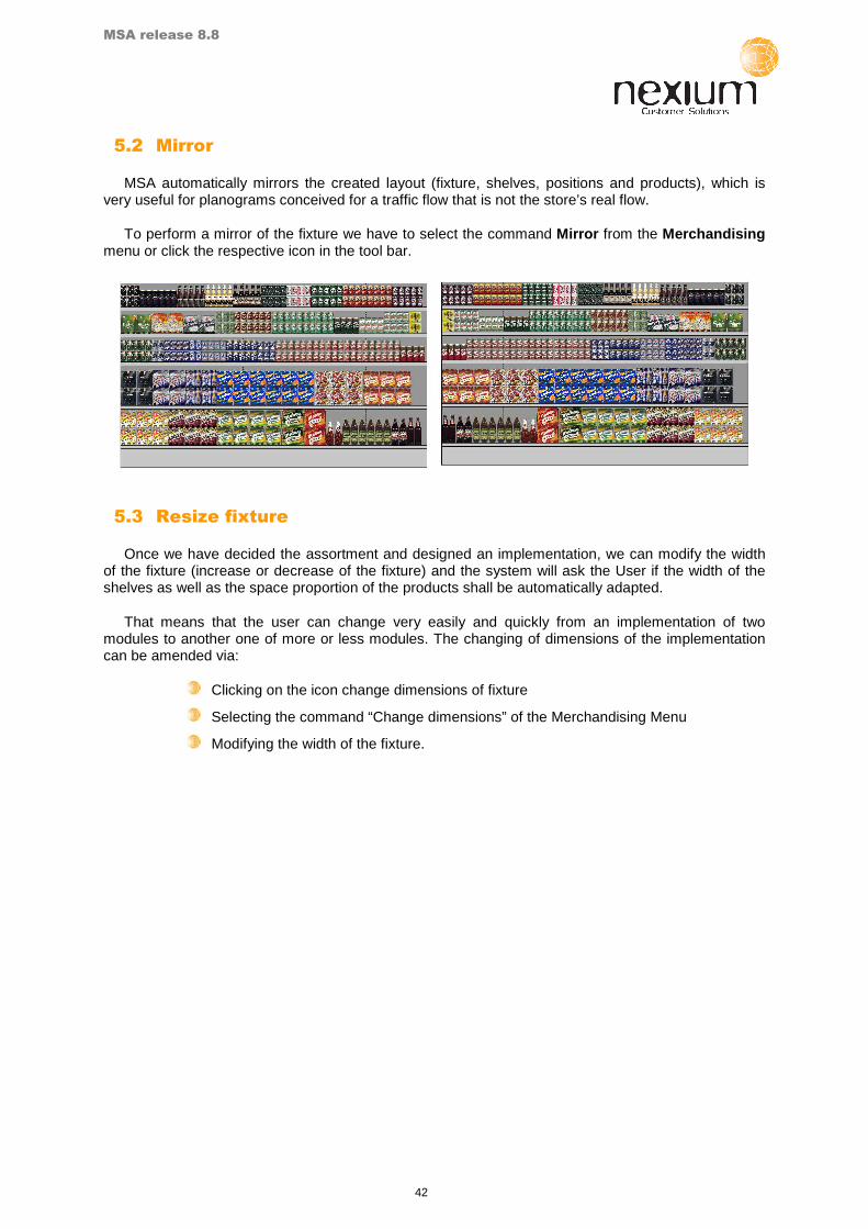
5.2 Mirror
MSA automatically mirrors the created layout (fixture, shelves, positions and products), which is very useful for planograms conceived for a traffic flow that is not the store’s real flow.
To perform a mirror of the fixture we have to select the command Mirror from the Merchandising menu or click the respective icon in the tool bar.
5.3 Resize fixture
Once we have decided the assortment and designed an implementation, we can modify the width of the fixture (increase or decrease of the fixture) and the system will ask the User if the width of the shelves as well as the space proportion of the products shall be automatically adapted.
That means that the user can change very easily and quickly from an implementation of two modules to another one of more or less modules. The changing of dimensions of the implementation can be amended via:
Clicking on the icon change dimensions of fixture
Selecting the command “Change dimensions” of the Merchandising Menu
Modifying the width of the fixture.

43
Inventory model
6.1 Characteristics of the model
The inventory model is based on a statistical model that includes all the different variables affecting the calculation of the optimum stock level for each of the items included in the fixture being analysed. The system takes into account: the effective opening hours of the store, the replenishments made over the week, the variability of the demand, service improvements, etc.
To create / modify the parameters of the model that MSA uses in calculating the target stock, we have to choose the menu Model from the Program’s Menu Bar.
When entering the window for the Model the system asks us for information on the different variables involved in the mathematical analysis undertaken by MSA for determining the advisable stock levels by product.
Opening/closing times: this table must contain the times when the store is effectively open to the public.
Chapter
6

MSA release 8.8
44
Demand per day: this states the percentages of sales made by the store on each of the days of the week over the total weekly sales (100%). MSA includes a window that displays the summary total of the figures included in the system. When all the figures corresponding to the seven days of the week are included the summary total must be equal to 100. If not, MSA reports the error and requests the data to be modified.
Demand variability: this determines the fluctuation over different weeks of the average level of sales of an item or market. To determine the value of this variability the deviations are calculated in terms of the absolute value of each of the weekly sales observations over the average, this is divided by the number of observations and a calculation is made of the percentage it represents over the average value. This is explained in the following example:
INVENTORY MODEL
Product A Weekly Sales:
Week 1 Week 2 Week 3 Week 4
10 15 30 20
Unit Sales = (10 + 15 + 30 + 20) / 4 = 18,75
Average absolute deviation = (10-18,75+15-18,75+30-18,75+20-18,75)/4=6.25
Demand Variability % = Average absolute deviation / Unit Sales = 33%
= 6,25 / 18,75 = 33%
IMPORTANT: For calculating the weekly sales it is recommended to use at least 4 months of history in order to take account of the demand variability.
Consumer satisfaction level: this expresses the percentage of consumers who have historically had their purchasing needs provided in the store being analysed. The consumer satisfaction level can be easily seen from situations of out of stock, from the poor location of products or from deficient signing of the fixture in the store.

MSA release 8.8
45
The satisfaction level determines the potential demand for a product, brand or item since the sales made for each item do not take account of consumers who did not buy it. So, we determine the potential demand for a product as:
POTENTIAL DEMAND = PRODUCT SALES / SATISFACTION LEVEL * 100
Service improvement: improvement target in meeting the needs of consumers who access the fixture.
Fixture replenishment: this table includes the number of replenishments made per week as well as the day and time of replenishment of products.
If we activate the option Automatic calculation, MSA will determine the day and time of the week on which replenishments must be made so that we can optimise them.
Once the above variables have been included in the system and if we click the key “Next”, MSA permits selection of the application methodology for the stock calculation model, restricting it exclusively to the scope that we wish at any time: total fixture, for a category, a family, a manufacturer or an item.
The program has different options for calculating the target stock:
Function of the demand: bearing in mind all the parameters analysed in the model such as opening/closing times, variability and demand per day, satisfaction level and fixture replenishment, the system calculates the optimum stock that the product should have in the fixture in order to meet the demand for it.
Days: by including a figure, such as 3, we force the model to have sufficient stock for meeting the demand for three consecutive sales of greatest sale.
Cases: this is the same concept as that in the previous paragraph, but considering the number of product replenishment cases to have on the shelves.
Constant: the user manually determines the number of units of product that there should be on the shelves.

MSA release 8.8
46
If we have the target stock calculation activated as a function of the demand and we introduce a value in Days, Cases or Constants, the system will take as the target stock the greatest value of stock calculated by the system in each section.
MSA permits a different value to be introduced at the Family, Manufacturer or Item level for the stock calculation models defined by the user: constant, days, cases. This entire process is done by at all times selecting as the target stock the most restrictive value from those calculated by MSA.
By clicking on the Family / Manufacturer or Item controls, those elements with a model defined as [.] will appear at the end of the list.

47
Analysis
7.1 Quadrant analysis
The Quadrant analysis positions the different segments, products or items making up the planogram within a system of axes defined as a function of the variables considered and the calculation method of crossing them (mean, weighted mean or constant values).
MSA facilitates quadrant analysis to be performed from groupings corresponding to the segment or manufacturer to those for item, in which case the user can determine the reference frame and focus it on the manufacurer, segment or total category.
Once the analysis level and the reference frame have been selected, a determination will be made of the variables marking the positioning of the items, segments or manufacturers within each of the quadrants.
Thus, a determination is made of the variables X and Y for the axis system that is designed, a third variable which will represent the size of the bubble and the calculation methods used for positioning the central point of the axes, which can be:
Mean: arithmetical mean value of the variable considered in all observations.
Weighted mean: weighting criterion for the space occupied by the item, manufacturer or segment.
Chapter
7

MSA release 8.8
48
Constant: values to be determined by the user.
Once the variables have been selected and the axes determined, the following screen graphically displays the location of each item, manufacturer or segment within the quadrants in the right-hand part of the screen, with the left-hand part showing its location in the planogram; each product is coloured according to its location within the established axes.
The options in the lower part of the screen permit printing of the coloured plan by quadrants, as well as of the three-dimensional chart, and it permits acceptance of the situation generated by the analysis, with which the planogram screen is returned to, with the products being coloured according to their location in the different quadrants.
If we click with the mouse on each bubble an information window will appear stating which product is being worked with and the values of the variables in the chart.
SUMMARY QUADRANT ANALYSIS
Menu Analysis/Quadrant analysis or click the quadrant analysis icon.
Select the analysis level, Manufacturer, Segment or Item.
If we select item, determine the reference frame (e.g.: analyse the items of SEGMENT A).
Select variables for the analysis.
Print, OK (the products become coloured according to their positioning on the generated axes), Cancel or Print.
MSA release 8.8
49
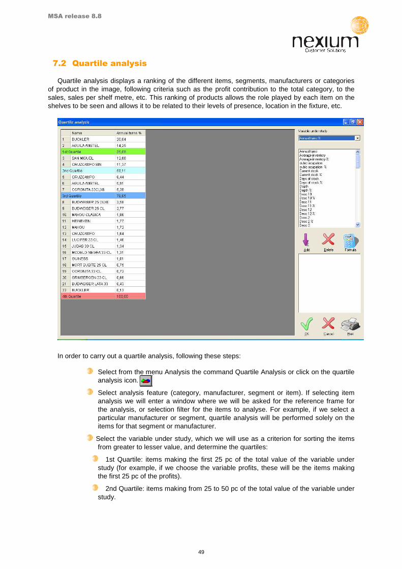
7.2 Quartile analysis
Quartile analysis displays a ranking of the different items, segments, manufacturers or categories of product in the image, following criteria such as the profit contribution to the total category, to the sales, sales per shelf metre, etc. This ranking of products allows the role played by each item on the shelves to be seen and allows it to be related to their levels of presence, location in the fixture, etc.
In order to carry out a quartile analysis, following these steps:
Select from the menu Analysis the command Quartile Analysis or click on the quartile analysis icon.
Select analysis feature (category, manufacturer, segment or item). If selecting item analysis we will enter a window where we will be asked for the reference frame for the analysis, or selection filter for the items to analyse. For example, if we select a particular manufacturer or segment, quartile analysis will be performed solely on the items for that segment or manufacturer.
Select the variable under study, which we will use as a criterion for sorting the items from greater to lesser value, and determine the quartiles:
1st Quartile: items making the first 25 pc of the total value of the variable under study (for example, if we choose the variable profits, these will be the items making the first 25 pc of the profits).
2nd Quartile: items making from 25 to 50 pc of the total value of the variable under study.

MSA release 8.8
50
3rd Quartile: items making from 50 to 75 pc of the total value of the variable under study.
4th Quartile: items making from 75 to 100 pc of the total value of the variable under study (usually called “range base products”, these are the a priori candidates for eliminating from the range if we have to reduce it).
Select other variables that we can use for making more advanced comparative studies in the lower part of the screen, adding (->) or removing (<-) variables to and from the report.
Print the report or analyse the position of the products in the fixture, according to the quartile where they are located.
In the quartile display screen for the fixture, we can:
Print the planogram or the quartile report.
Accept the analysis, with which we will have the planogram coloured by quartiles (for the products to return to their original colours, we simply have to select view by blocks, units, shapes or digitalised images).
SUMMARY. QUARTILE ANALYSIS
Menu Analysis/Quartile Analysis, or click on the quartile analysis icon.
Select the variable under study in the upper window (on which the quartiles are going to be created).
Select the other variables to introduce in the report in the lower part of the window.
OK. MSA will generate the planogram colouring the different products according to the quartile where they are included.
Print.

MSA release 8.8
51
7.3 Spectral Analysis
Using spectral analysis we can obtain a planogram that facilitates a very intuitive analysis of our implementation based on several variables. By colouring each product according to the weight it represents within the set of variables you will be able to easily understand the current situation of each product (based on the variables you had selected)
You can access this option via the menu Analysis � Spectral Analysis or using the direct icon in the tool bar. Once you have selected the respective option the following screen will appear:
In the upper part of the screen the colour spectrum that will be used in the analysis will appear. You can define two colours, one for the mayor value another one for the lowest value. MSA will either calculate the rest of colour that will represent in-between values, or you can opt for a third colour to represent the intermediate values. For this second option select “Define colours of intermediate values” and a third colour button will appear automatically.
In the mid part of the window the user shall define the product variable on which the analysis is to be based. To do so select the option “Select variable to be used” and the variable that you indicate in the lower drop down menu. If you want to create a new formula using a combination of variables, activate the option “Formula” in order to define it.
After clicking the button “Formula” the following screen will appear:
In the upper part of the screen the name of the formula is to be introduced. The field below will show the formula that is being created.
In the drop down list of variables you will find all the variables that can be used. Next to it you can see the operations that are to be made in case the products shall be grouped.
On the right hand side of the screen you can see the digits, operations and some control buttons for the formula. In order to enter a variable, select it from the list and hit the Enter button of the keyboard. If you need to delete only the thing you

MSA release 8.8
52
have entered, click on the green button with the arrow pointing left. The red C button can be used to delete the whole formula.
Once you have finalized the formula click on “Accept” to use the formula or “Cancel” to quit.
Finally, you can define on the main screen of the Spectral Analysis if the analysis will include all items or if the programm shall first apply groupings. This second option is accessed via “Carry out analysis grouping by” and selecting the grouping variable of the product.
Once you have entered all parameters of the analysis click on “Accept” so that they are applied on the colours of the products, or “Cancel” in order to delete the changes and leave the feature without carrying out any action.
7.4 Over / Understock
The over / understock analysis permits differentiation between products with sufficient units on the shelves for meeting consumer demand and those in a situation of product deficit on the shelves, for which shortages at the point of sale service to the consumer could occur, thus leading to lost business opportunities for the category under analysis.
We can access the over / understock analysis by means of the icon or via the menu Analysis / Over understock.
The system displays the products in the fixture by means of the following colour key code:
Products in red: products with a deficit of units on the shelves.
Products in green: products with excess stock in the fixture.
Products in white: products balanced in terms of stock on the shelves.
The product units are sufficient for meeting consumer demand or they fall between that balance and the overstock percentage accepted by the user.

MSA release 8.8
53
Appearing in the lower part of the window are statistics associated with the over and understock situations such as metres and percent of space occupied by products as stock excess, along with lost sales deriving from products with a deficit of stock on the fixture.
This screen contains two options:
Adjust stock.
Fill up the space available in the fixture.
7.4.1 Adjust Stock
This leaves each product with the stock that the system regards as optimum for meeting the demand, taking into account the restrictions and parameters included in the inventory model.
There are two options in the adjust stock function:
Adjust stock to the maximum.
Fill up with products, with two options:
Fill up to the maximum in depths.
Fill up to the maximum in stacking.
7.4.1.1 Adjust stock to the maximum.
This option gives each product the optimum stock and takes no account of merchandising factors such as stacking or logistic conditions such as filling up the fixture to the end (it does not stack product even if it were to fit and does not fill the entire shelf in depth with product. It merely stacks and fills as far as reaching the target stock).
7.4.1.2 Fill up with products:
This option fills the available space:
In height (piling up product if possible).
In depth (filling up to the maximum in depth). Even when the target stock is exceeded with this option.

MSA release 8.8
54
If we have items in understock these will appear in the lower part of the fixture in live images (if we do not have live images available to us, the product will appear in units with its colour).
By dragging the products to the fixture, the system will automatically place the necessary product so that it ceases being in understock.
7.4.2 Filling up the fixture.
The system automatically divides out the available space among the planogram items (making the total available space of the fixture 100 pc) in line with one or more of the following division criteria (the option exists of giving a different weight to each variable in order to obtain a weighting division criteria plus one or other variable):
Unit sales.
Sales value.
Profit.
Share.
In the lower part of the line the items needing more space than they currently have will appear. The products will be shown in digitalised image (if we do not have digitalised image available, a product unit will appear in the colour defined in the database). In the left-hand part we have the main information on the selected product.

MSA release 8.8
55
When dragging the product to the fixture, the system will automatically assign it the space that the item requires.
7.5 Filling up the shelves
7.5.1 Complete piece of fixture
Same function as filling up the shelf in the case of Over/Understock.
7.5.1.1 All the shelves
MSA calculates the excess space for the shelf in each of the shelves in the planogram, and adds facings for the products located on this shelf in terms of the weight given to the selected variables.
7.5.1.2 Per Shelf
This shares the remaining space on a single shelf selected by the user. To perform this operation, MSA calculates the remaining space on the shelf and adds facings to the products located on this shelf in terms of the weight given to the variables selected.

MSA release 8.8
56
7.6 Reports
The reports function of MSA is accessible via the respective icon in the tool bar or vie the menu View/ Reports. This is the first screen that you will see:
Here the user can generate the structure of the report that we want to create, and can save various types of reports that can be used in different reports that can be used for different planograms.
Using the window situated in the lower right part and using the arrows placed in the middle as well as the options “all” or “none” you can design customized reports that are most interesting for each of the analyzed categories.
Apart from that, the user can prioritize the order of the listed products and their characteristics. Clicking on the button “Sort” you will see the screen shown below.

MSA release 8.8
57
Here you can select the order of appearance of the products in the reports, based on one or two variables. The priority of collocation will be shown in the column called “Nºorder” where you also find the box that needs to be checked in order to activate the prioritization. Right from it you can include a subtotal (subtotals will be made for each change in the value of the variable.)
For example if you select the variable Segment, the program will calculate the subtotals for each segment of variables in which an operation had been selected (sum, count or average).
MSA offers the possibility to calculate variables that have not been predefined by the system via an easy to use formula generator which reflects the operations available for creating a new variable. These new variables can be filed in different reports, so that they can be used in different planogram so that you only have to create the formula once.
The procedure for creating new variables is as follows:
Select the name of the variable you which to create
Select the first variable and press enter
Select the operation (+, -, x, /).
Select the second variable and press enter again
Once you have entered the formula, click accept and the new variable will be available for our reports
SUMMARY: REPORT GENERATION
Access: Menu View/Reports or via the icon in the tool bar
Choose the variables that shall be used in the report using the options that appear in the lower part of the screen.
Sort them if necessary
Save the report.
Menu: File/print
Select the report you created

MSA release 8.8
58
7.7 Economic summary:
To carry out an economic valuation of the planogram, we have two possibilities:
Click on the summary icon.
Select the command Summary from the analysis menu.
In the column Current, we have the economic summary of the planogram that we are recreating, and in the Target, the data corresponding to a planogram with the optimum stock recommended by the inventory model, giving a consumer satisfaction target.
In this window we can:
Copy the information to the clipboard.
Print it.
7.7.1 Definition of the variables included in the analysis:
The following variables will be available in the analysis:
Profit: Unit Margin x Number of units sold.
Profit / m3: Profit per cubic metre of product placed in the fixture.
Profit / shelf m: Profit per occupied metre of product placed in the fixture.
Target profits: Target Sales x Unit Margin
Lost profits: Lost Units x Unit Margin
Shelf space m: Fixture occupied (shelf space occupied by products in the width of the shelves).
Volume m3: Volume occupied in the fixture by the products (width x height x length)
Facings: Number of horizontal facings that a product has in the fixture.
Average inventory: Weekly Average number of stock units of product in the fixture.

MSA release 8.8
59
Unit margin: Sale Price - Cost Price
Markdown: Markdown = (Sale price - Purchase price)·100 / Sale price
Markup: Markup = (Sale price - Purchase price)·100 / Purchase price
Annual rotation: Number of times that the inventory fitting in the fixture turns over in one year.
ROII Cost: Profitability ratio, measures the total number of times that we recover each monetary units invested if we were to meet 100 pc of the demand. We value the inventory at cost price
((Sale price - Purchase price) x Demand x 52)/(Average inventory x Purchase price)
ROII Target cost: Profitability ratio, measures the total number of times that we recover each monetary unit invested in line with target sales. We value the inventory at cost price.
((Sale price - Purchase price) x Target sales x 52)/(Average inventory x Purchase price)
ROII Price: Profitability ratio, measures the total number of times that we recover each monetary unit invested if we were to meet 100 pc of the demand. We value the inventory at sale price.
((Sale price - Purchase price) x Demand x 52)/(Average inventory x Sale price)
ROII Target price: Profitability ratio, measures the total number of times that we recover each monetary unit invested in line with target sales. We value the inventory at sale price.
((Sale price - Purchase price) x Target sales x 52)/(Average inventory x Sale price)
Current stock: Number of products placed in the fixture.
Target stock: Number of products that should be in the fixture for fully satisfying the demand.
Lost units : Difference between demand for the product and stock in the fixture.
Sales value: Sale price x Sales of units
Target sales value: Sale price x Target sales of units


61
8.1 Charts
Accessing via Analysis/Charts the user can open a predefined graph or create a new one. If you select NEW the following screen will appear, showing the three different types of graphs that are available (bars, pie, bubbles)
Independently of which kind of graph you choose you can select either “all products” which includes all those that have been placed in the fixture and those of the warehouse or the database or “Just the products placed on shelf”. Now you can either click directly on the respective graph or proceed to the “Advanced” option. Below we will explain the standard option.
8.1.1 Bar chart
Choosing the bar chart option the following screen will appear, where you can choose up to three different variables to be included in the same graph.
Within these variables you will find a new field called “occupation”. This variable will show three measures: cubic occupation, shelf occupation and exposition (also available in percentage). The following planogram shows you how these variables are to be interpreted:
Chapter
8

MSA release 8.8
62
One could also select one operation for each variable in the field “operation variable” in order to view the accumulated data, the maximum, the minimum or the average.
In the field “level of study” the user shall select the variable that is to be represented in the graph. Clicking on the tabs you can see all the possibilities. The following graphs show an example of a bar chart carried out “by manufacturer” and another one “by segment”
By Manufacturer: By Segment: Estudio por Fabricante
Cuota %
Facings %
Volumen m cúbico %
SAN MIGUEL
MAHOU
HEINEKEN
GUINESS
CRUZCAMPO
AGUILA
42
32,2
29,3
2321,9
20,2
10
14,5
19,2
9
2,82,1 2
7,1
5,3 5
18,4 18,9
9
3,2
5
Estudio por Segmento
Cuota %
Facings %
Volumen m cúbico %
SIN
ALC
OH
OL
NAC
IONA
L
IMPO
RTA
CIO
N
53
42
36,835
43,8
49,3
12
14,1 13,9
If no variable has been selected, an error message will appear, as you have to select at least one variable in order to perform the calculations.
Once you have selected all the necessary field click on the icon “next” so that the graph appears. From this screen you can access the configuration and printing options of the graph as well as save it.
Cubic
Shelf Exposition

MSA release 8.8
63
This is the configuration screen accessed via the respective button:
TITLE: Here you can input the information that shall be shown as a heading of the graph and the font of the text. IN order to activate the title you need to check the box on the left of the button.
LEGEND: Via this button the user can indicate where the legend of the graph shall appear, choosing between four options (above, below, left, right). Again the option is activated by the check box.
X AXIS: If you activate this option, the level that has been chosen to create the graph will be shown on the screen (name, SKU, …) Again you can change the font of the text.

MSA release 8.8
64
DATA: Decide if you want to show the data of the selected variables in the graph.
TEXT: This is a comment function where you can include a text in the graph that is shown or not depending on the activation of the left check box.
Apart from that you can activate “division lines” (show in the background of the graph), “scale” (to be shown on the left) as well as “pattern” and “average”.
The option “Limits” in the mid part of the screen refers to a maximum and minimum value of the main variable, so that only those items that are within these limits of the variable will be shown in the graph.
Activating “Difference” and the options Max, Min or both, those items that represent the minimum or maximum value will be marked with a different pattern.
There are two fields for “Background”. The left one is used to change the background of the bars, the right one changes the background of the whole graph.
8.1.2 Pie chart
If you click on the icon of the pie chart, a screen very similar to the one of the bar chart will appear, with the difference of having only one field for choosing a variable, the operation for this variable and the level for which you would like to perform the study.
It’s mandatory to select a field in order to calculate the graph, if not the following error message will appear:
The following graph shows a pie chart made on the level of “name”, all of which appear in the right part of the chart and represents accumulated sales.

MSA release 8.8
65
By clicking on configuration you will access to the following screen:
TITLE: Here you can input the information that shall be shown as a heading of the graph and the font of the text. IN order to activate the title you need to check the box on the left of the button.
LEGEND: Via this button the user can indicate where the legend of the graph shall appear, choosing between four options (above, below, left, right). Again the option is activated by the check box.

MSA release 8.8
66
TEXT: This is a comment function where you can include a text in the graph that is shown or not depending on the activation of the left check box.
Activating “Difference” and the options Max, Min or both, those items that represent the minimum or maximum value will be differentiated by a pattern. The decimals that shall be shown in the data can be amended via the field “decimals”. In “pattern” you can change the colours of the sectors using a pattern and in “background” you can change the colour of the background of the graph.
8.1.3 Bubble chart
Choosing this graph the user will access a screen of three different variables that are necessary to create a bubble chart. They refer to the X and Y axis and the third dimension (that will be represented by the size of the bubbles)
Other than the other graphs this one needs to have all three fields defined in order to show the data. Again you find the fields for the level of study and the operations of the variable. In case you click the next button without having selected anything you will see the following error message.
Once you have finalized the definition process you can access the graph (see below). If the user clicks on any on the bubbles an information window will appear where the value of the three defined fields will be shown.

MSA release 8.8
67
This is the configuration screen:
TITLE: Here you can input the information that shall be shown as a heading of the graph and the font of the text. IN order to activate the title you need to check the box on the left of the button.
LEGEND: Via this button the user can indicate where the legend of the graph shall appear, choosing between four options (above, below, left, right). Again the option is activated by the check box.
TEXT: This is a comment function where you can include a text in the graph that is shown or not depending on the activation of the left check box.
DATA: Activating this button the data selected in the previous step will be shown.
In the “pattern” field the user can change the colour of a bubble for a patterns and in “background” you will change the colour of the background.

MSA release 8.8
68
8.1.4 Advanced options
Once you have entered the graphs section via Analysis/ graphs the main screen provides the option “Advanced”. Clicking on it opens a screen where the user has the possibility to restrict the SKUs used on each of the graphs. The window consists of three sections, each dedicated to different restrictions: modules, heights and products. You can select one by one are all at a time. If you click on “simple” the program will return to the initial graphs screen. Once you have made the desired selections click on the icon of the kind of chart you wish to create.
8.1.4.1 By modules
Having chosen this options the user can indicate on which module he wants to base the study, which is the first and which the last module. For example, if you only want to include the second module, it needs to be selected as first and final module.
The second option is to select “measures” in order to do the selection based on measurements. The fields will change to admit the measure that has been assigned in File/Options/Configuration (be default it’s centimetres). Note that if the final value you put is smaller than the initial value, no products will appear in the graph.
8.1.4.2 By heights
You can select from which to which type of fixture (chest, shelf or hook board) you want to perform the study. In the two fields on the left you need to select the initial and final element, in the fields on the right the name of the respective element as there may be various fixture elements of the same type. Doing this the program will only analyse those products that are placed on the indicated fixture elements
If you activate the option “by measures” you can tell the program to analyse only those products that are placed within some determine measures. The measures will adapt the format of the program, by default centimetres) although you can change it in Options/configuration. If you final measure is lower than the initial one, no products will appear in the graph.
8.1.4.3 By products
There are two options: the first analyses only those products that have been placed on a shelf, not taking into account the ones in the warehouse or the database (“Only the products placed on shelf”). The second is called “Include only the following…”. This option will activated the field “Include” which grants access to another screen where you can select the items to be included.

MSA release 8.8
69
The window is made up of three parts. “SKUs to be included” facilitates the possibility to include items that are grouped by a common value, like for example all SKUs coming from the same manufacturer. In the drop down menu “variable” you can access all available variables of the database by opening the menu on the right hand side. In “value” you will define the desired value the that shall represented in the report.
Once this is done, you click on “include” and the SKUs that have been selected will appear in the lower part of the screen. The sector “applied rules” shows the constraints and selections that have been made. On the right hand side you can delete a rule or selection of products or delete all products at a time. The option “insert all” allows to include all SKUs at a time.
Another possibility of selection is to click on the respective SKU in the right hand part of the screen (“SKUs to b excluded”). By this you don’t have to look it up in the tabs of “SKUs to be included”.
In the part of “SKUs to be excluded” all items of the planogram will appear in case none of them has been included, independent of if they are placed of not. As more and more items are being included they disappear from the right screen but they can still be selected by clicking the tab of the field of value and variable. After having done so, the user shall click on “exclude”. Just as in “references to be included” you can select them by clicking on the item on the left hand part of the screen.
8.2 Print charts
Once you have created the graph a printing button will appear, that leads to the following screen. Here the user can adjust the margins and configure tha printer (if it is a vertical of horizontal print, the type of paper, etc.)

MSA release 8.8
70
8.3 Save and open graphs
The user can save the graph under an extension “gph”. The graph that is saved will work like a template, that is, it can be opened with other planograms to be used with their data. If the graph had some rules attached to it (advanced graph) it might happen that they are not accepted in some planograms, as they work with a different database. If this happens the graph will appear blanc, without data.
8.4 3D View
The 3D functionality allows to visualize the planogram in 3 dimensions, providing a more realistic view that facilitates the validation of the final implementation.
You can access the option via the tool bar clicking on the icon: “ ” that is located as follows:

MSA release 8.8
71
You can also access via the menu “View/ 3D View”, as shown in the following figure:
Once you have selected the 3D view you will see the following screen:

MSA release 8.8
72
The initial 3D view of the planogramm displays the front view, simulating an observer situated in front of the fixture, centred and at medium height of the shelves. This observer can be moved using the control of “figure 1”, whereas his point of view can be moved using the control shown in “figure 2”
Figure 1 Figure 2
Figure 1: MOVING THE OBSERVER:
The observer moves forward by pressing the upward arrow ↑ of the keyboard cursors or clicking arrow number 1 shown in Figure 1.
In order to let the observer move back, us the downward arrow ↓ of the keyboard cursers or click arrow number 2 of the control shown above.
To move the observer to the right, press the X key of the keyboard or click arrow number 3.
To move the observer to the left, press the Z key of the keyboard or click arrow number 4.
The observer will turn to the right without changing his position using the rightward key � of the keyboard cursers or via the arrow number 6 shown in figure 1.
The turn to the left without changing position is effectuated by using the leftward key → of the keyboard cursers or arrow number 5 of figure 1.
Figure 2: MOVING THE VIEWPOINT
You can move the viewpoint upwards pressing the “Pos 1” key of your keyboard or using the arrow 1 of Figure 2.
To move the viewpoint downwards press the key “end” of the keyboard of arrow 2 shown above.
In order to rotate the point of view downwards without changing the position you can use the key “page down” of the keyboard of arrow 3 shown in Figure 2.
To move the view upwards without moving the position use the key “Page up” or arrow 3 of Figure 2.
In the lower part of the main screen of the 3D view you find three different buttons: export image, configuration and Exit.

MSA release 8.8
73
The button “Export image” offers the option to save the actual view of the planogram in 3D as a “.JPG” file. Clicking on it you will access the usual dialogue window used to save the file in the desired folder under a certain name.
Via the “Configuration” button the user can amend the different viewing options and the 3D motor used by MSA. The following screen will appear after clicking:
The screen is divided in three sections: Current acceleration, Video and MSA.
The section Current acceleration provides information about the “manufacturer”, “engine” and “version” concerning the hardware characteristics of the 3D galleries that are used with the selected options.
In the “video” section you can decide about four options:
Render: Choose between “hardware” acceleration (“OpenGL” Option that used the graphic card to carry out the maximum performance of calculation, liberating the processor) or “software” acceleration (all simulation calculations are performed by the processor). Normally the graphic card is faster than the processor in calculating 3D views, therefore it is convenient to select the OpenGL option whenever possible. Nevertheless, in some cases the drivers of the card may not be updated or are

MSA release 8.8
74
having a problem that causes MSA to become unstable. In this case the user should select “Software”.
Bits per point: Here you can select either 16 or 32. The 32bits option allows to display the images more realistically, while “16bits” allow to save memory during the visualization.
Colour Depth: Again you can select either 16 or 32. The 32bits option allows to display the images more realistically, while “16bits” allow to save memory during the visualization.
Use shadow: If you activate this checkbox MSA will use ambient lighting by default in order to make the view of the planogramm more realistic, if you don’t use this option the lights will not be used, instead you will see drawn lines around each 3D element.
In the “MSA” section you can decide about four options:
Generate texture if no image exists: If there is no image available for any of the sides of the product this option generates an image with the current colour of the product, so that you can see the different products existing in a position.
Use images: This option activates the use of images on each side of the products. If it is deactivated you will not see the top and laterals images but a colour of each product.
Resolution of the textures: You can choose between the resolutions “32x32“, “64x64“,“128x128“ and “256x256“ that refer to the quality of the product images. “32x32“ is the worst quality that uses fewest memory and “256x256 “the best quality that needs most memory space. You should choose the resolution taking into account the available resources of the equipment on which you execute MSA.
Quality of the textures: You can select either “Best”, “High”, “Normal”, “Low” and “Worst”. All options directly affect the real-time performance of the 3D visualization as well as the quality in which the whole planogram is displayed. “Best” is the maximum quality with maximum hardware requirements and “worst” is the minimum quality and minimum. You should choose the quality taking into account the available resources of the equipment on which you execute MSA.
Via “Cancel” you quit the screen without effectuating any of the changes you made in the options and “Accept” applies the amendments. Possibly MSA will need to re-calculate the 3D objects in order to apply the changes.
Finally, on the main window of 3D view appears the button “Exit” that closes the window in order to return to the MSA planogram.

75
Printing
Via this option the user access the following window, allowing us to print:
Planograms.
Charts.
Reports.
Reports and charts.
Planograms and charts.
Planograms and reports.
By clicking the button Properties, the printing controller for the predetermined printer is opened, offering the following modifications:
Orientation of the sheet.
Paper size.
Printing quality.
To change the predetermined printer we click on control name and select the new printer from among those installed in the system.
Chapter
9

MSA release 8.8
76
IMPORTANT: If the rulers are activated on the screen the planogram will be printed with rulers.
In this screen the user can define the title, subtitle or text (comment) that shall appear in the planogram.
By clicking the font button in the title / subtitle or text, the font and text size can be selected. With a simple click from the mouse the user can add the date, time, traffic flow (in the planograms) or legend (if we are printing a quartile chart or planogram or one on over / understock).
By default, planograms are printed on one page, but they can also be printed by sections (making a click on the edge of the sections and putting the number of sections to print per page).
9.1 Reverse mode
The reverse mode is used to print shapes with the background of the fixture in white, increasing the perception rate and reducing printer ink consumption, by clicking on INVERT
Normal Mode Reverse Mode

MSA release 8.8
77
9.2 Printing by modules
To print a planogram by modules activate the “modules” option. If this option is activated by clicking "Print", the following screen will appear in which the page to be printed can be selected.
9.2.1 Mark the limits of the modules
Now MSA allows the modules to be marked with discontinuous lines, on the shelves and on the products to be able to differentiate the limits of the sections of the fixture more clearly.
9.3 Adding logos
When printing the fixture, up to three company logotypes can be added, by clicking the “logos” option the following screen appears:
The logos are added automatically in the lower part of the page. The file formats must be “Windows BMP”. To select the files click the “Browse” button.
REOMMENDATION CATEGORY STRUCTURE

MSA release 8.8
78
9.4 Select font and height
In case the user selects a printing option that includes texts or tables, MSA provides two combos for the selection of text format. From the initial printing screen you can select the type of font using the drop down menu at the lower part of the screen. The field “height” can be used to indicate the millimetres of the character in the print-out.
Font Height

79
Configuration
Within the configuration command in the menu File, you can customize the system by choosing between the following options:
The dialog window of configuration will show various tabs, each one dedicated to the customization of certain functionalities of the system.
10.1 General configuration
On the first tab of configuration (show n above) the user can access the following characteristics of the program:
Dimensions: measurement unit that is used when entering MSA data.
Language: MSA allows the language to be changed in the work session.
Image directory: The directory in which MSA will search and save the images and silhouettes assigned to the products will be indicated in this field. By default, the
Chapter
10

MSA release 8.8
80
directory will be "images", which will be located in the directory in which MSA was installed.
Labels: the information that will appear on the product labels is defined in this section. The field that will appear on the upper label will be selected by means of the first control and the lower label using the second control. The command "Font" will be used to select the letter type and its size. By activating the command "size adjusted", if the label does not fit on the product, MSA will reduce its size until it adjusts to its surface.
Information window: the variables selected here will form part of the information
window of the planogram that appears when clicking the icon; click the icon again to disable it.
Configurable fields in the product lists. Two fields can be selected that are needed to appear in the product lists that are shown throughout the program.
10.2 Images
If we select the next tab of the configuration screen, we can adapt the following characteristics to our specific needs:
Images directory: This field indicated the directory in which MSA will search for and save the images and shapes assigned to the products. The default directory is called “images” and will be found in the folder where the MSA software has been installed.
If you chose “Use front image by default” the programm will use by default the front image of the product.
Transparency: With this option you can determine a certain colour to be transparent in the product images. Here you can choose the colour by selecting its three basic components: red, green and blue.
The transparency function is very useful as the shape of the images will be seen much better if the background is transparent instead of grey or any other colour which will cause the appearance of a rectangular shape behind the product.

MSA release 8.8
81
In order to help the program identify the colour that is to be made transparent, you need to paint the background of the image in any imaging program in a colour that does not appear in the graph itself, e.g. bright blue or using the same green that appears by default. Once this is done, the program and the option “make this colour transparent “ is activated the program will automatically modify each image containing the respective colour
Please note that the images need to be saved in format bmp.
You select the colour using the fields of the basic colours red, green and blue, where you can move the cursor until you reach the colour you need. The intensity of the colour can also be chosen in the right hand fields. Cero corresponds to very dark colour, 255 is the brightest colour.
10.3 Descriptors
The name of each of the descriptors can be customized, by changing the text that defines it.
For example: if the date on which the product was updated is stored in the first descriptor, the "Descriptor 1" text can be substituted by "Date of updating", so that any MSA window, data on reports or on the analyses will be shown with the field name "Date of updating".
MSA allows a specific name to be given to each of the 12 descriptors. The variation with respect to previous versions is that each name is stored in the system register, allowing new updates of the application to be made without losing the value given to them.
On clicking on "ACCEPT", the new definitions will be stored in the language active at that moment.
10.4 Colours and Colouring by Groups
With MSA you can give a name to the colours for a better and more exact identification of these when they are assigned to the products. Furthermore, the colours assigned to a planogram are automatically stored without any intervention of the user when colouring is used by groups to later colour other planograms always using the same colours.

MSA release 8.8
82
To give names to the colours, it is necessary to enter the options screen (this can be accessed via the File menu and the Options sub-menu) and by clicking the Colours button the Define colours screen is obtained.
The window is divided into two parts, one for defining the names of the colours and the other for the definition of the colours from the options that appear in colouring by groups.
The definition of the names of the colours are found in the upper part of the window and adding, modifying and removing colours that have been created is permitted. The first time this is executed by MSA, if the names of the colours have never been defined, it creates the following pre-defined ones: Black, White, Light grey, Dark grey, Dark red, Red, Dark yellow, Yellow, Green, Light green, Bluish green, Turquoise, Dark blue, Blue, Violet, Fuchsia, Light pink, Brown and orange.
Use the Add button to create a new colour and the following will appear.
The name to be given to the colour is entered in the Name field. A rectangle will appear with the colour selected using the Choose colour button to the right of the Colour label.
For choosing the colour it will interact with the standard window used for all the Microsoft Windows applications.

MSA release 8.8
83
If the colour appears in the Basic colours, click on it and then on the Accept button.
In the case of it not being among the basic colours, the range of colours on the right part will be used. To choose the colour, click on the approximate colour required in the range and with the right vertical bar choose the brightness required, by raising and lowering the date. If the RGB components are known (Red, Green and Blue) of the colour or its Matrix, Saturation and Luminosity can be entered manually in the corresponding edition squares. Click the Accept button once the correct colour has been obtained.
If a colour is to be modified, this will be selected beforehand in the Colour selection box and then the Modify button is clicked.
The window for modifying colour is the same as that for adding except that the name and colour fields appear initialised with the colour selected.
To remove a colour this will be selected beforehand in the Colour selection box and the Remove button clicked.
NOTE: Each MSA language (Spanish, Portuguese, German, etc.) stores the names of the colours separately, as there is no reason for the same colours to exist among the different languages.
To add, modify or remove colours of Category, Manufacturer, Descriptors, Brands, Segments, Sub-segments, Sub-categories and Sizes, the one to be worked with will be selected first. For this, the field required will be selected from the Colour selection box (see below).
If you want to add a new colour for example to mark a certain brand the following screen is obtained.
The name of the category is entered in Name (in this particular case the Category has been selected, but the same could be done for Manufacturer, Segment, etc.) to which a colour has to be given. A colour that has been previously created is selected using Select, if the colour is not on the list the More colours button can be used to select an undefined colour (the window obtained is that shown above and the method of working on it is explained in the previous pages).
To modify the colour of a Category (or any of the fields possible), this is selected in the selection box that is found under that of field selection and clicking on the Modify button.
The modification window is the same as that for adding except that the name and colour fields appear initialised with the colour selected.
Removing the colour of a Category is selected in the selection box under that of field selection by clicking the Eliminate button.

MSA release 8.8
84
All these colours defined are those that the program will automatically use when accessing the colouring by groups window and which will be used in all the planograms.
10.5 Internet
MSA provides the possibility to configure various parameters for the creation of HTML pages. To access this option, select File/Option (it will only be available if you have opened a planogram or if you are creating a new one). Once the screen is visible click in the internet button in order to opened the following dialog window:
The first parameter that can be configured is the directory where the images will be found once they have been stored in the Inter/Intranet. If the images will be stored in the same folders as the HTML planogram select the option “same folder as the HTML files”. If the images were stored in another folder choose the option “In a different path” and specify the name of the folder in the respective editing field.
If you have selected the option “in a different path” it may happen that the image does not appear when the planogram is opened on the computer that had been used to create the HTML page. This is due to the fact that the internal link of the HTML page leads to the folder that has been chosen in the internet options and that the image may not yet have been saved in this place.
Another option that can be modified is the quality of the generated JPE images. 0% indicates the worth quality and the smallest possible size and 100% indicates the best quality and greatest filesize.
In the field “Variables included in the product report” MSA shows all those fields that will appear in the list that is obtained via the option “Publish on the internet/ Planogram with product list” therefore the user is able to select those to be displayed and where they are to be placed. In order to do so, click in the option “modify list” which will open the following screen:

MSA release 8.8
85
Here you can select either all fields or just some of them, using the arrows that are shown in the middle of the screen. The arrows on the right hand side of the screen can be used to change their position within the list.
10.6 Graphs
The following tab available in configuration is for the Graphs:
In the upper part of the screen you will find four sections: Title, Legend, Data and Text. If these fields shall appear on the screen of the graphs the user has to activate the respective check boxes. In Font you can change the size and the font.
In the lower part you can activate the “pattern” and they will be used in the graphs.
By activating the fields of “Differentiate minimum” and “maximum” those items that have the maximum and minimum value of the variable under study will be differentiated by a pattern independently of which graph you choose.
You can also indicate the number of decimals that shall be shown in the graphs and the colour of the background using the colour pallet.

MSA release 8.8
86
10.7 Filter
If planograms are imported from other Space Management systems, the user has the opportunity to configure several options that may be necessary to correctly effectuate the import.
The first option is to join all the contiguous shelves that are placed at the same height and have the same measurements.
The second option only joins those shelves where products have been placed in between two adjacent shelves.
The third one takes away all the fixed positions that had been placed in the original planogram.
The last option adjusts the height and width of the shelves so that no products are lost when the planogram is being imported.
10.8 Product Fields
The MSA options have been enhanced by a new tab “Product fields” that allows to define the name of each product files to be visualized in the program.
Just as in the previously explained cases, you access this new option via “File/Options” while you have a planogram opened and click on the tab “Product fields”.

MSA release 8.8
87
Each of the variables that can be configured has an editing field and a check box that indicates “default variable”. If you activate this option, the default name will be used in MSA, if you deactivate it the name specified in the respective editing field.
10.9 Store Database
Another new option available for personal configuration is called “Store Database” and gives access to the configuration of the automatic import of store data.
The options that can be chose are as follows:
When creating a planogram open the window to define the store data: If activated the user will be asked for the store data each time a planogram is opened.

MSA release 8.8
88
Use database: If this option is activated the program will try to read the store database that is configured in the following options and made available in MSA.
Database file: Refers to the file that contains the information of the store data. On the right hand side you fin the Browse button where you can browse the available archives and select the corresponding file.
Define fields: Here you can define the order of the store data fields that appear in the file. Clicking on this button will open the following window:
On the left hand side of the screen you will find all the store variables available that have not bee selected yet. On the right hand side you see the list of variables have been selected and the specific order of appearance in the file.
Apart of the store variables you can select the variable “none” that allows to ignore fields that shall not be included in the file.
Insert: Adds the variables selected in “Variables” to the list “Selected Variables”.
Take out: Excludes the variables selected in the list “Selected Variables” and takes them to the list “Variables”
Insert all: Includes all the variables of the list “variables” in “Selected variables” (Except the variable “none”)
Take out all: All variables included in the “Selected Variables” will be excluded and taken to the list “variables”.
The UP and DOWN buttons allow to change the order of appearance of the selected variables in the list.
If you click on Accept, the changes you made will be saved and you go back to the previous page, if you click on “cancel” all amendments will be ignored.
The next section of the configuration screen is dedicated to the definition of the import of the store data. You can choose between “Text file” and “Use the library of importation”. The difference resides in using a standard library included in the MSA installation that is compatible with the text files (delimited by a certain character) and use a different library, if the files do not adapt to the ones worked by the standard library.

MSA release 8.8
89
Within the option of “Text file” you can select the following options:
Separating character: Indicates the product that separates the fields within the file. Any character can be inserted in the field. In case it’s the tabulator you can activate it via the drop down menu.
Delete the initial and final quotes of the text fields: Determines that the motor deletes initial and final quote of each field.
Delete the initial and final blanks: Determines that the motor deletes initial and final blank spaces of each field.
Use the regional configuration of Windows for the decimals: Indicates to the motor of importation that the decimals of the numeric variables are not defined by the standard character “.” but by the one configured in Windows.
Import first row: Indicated to the motor of importation that the first file of the file contains data that needs to be taken into account.
Within the option “Use the library of importation” the user can “browse” in order to indicate the importation library be used.
Check the store fields when opening a planogram: If this option is activated, each time you open a planogram, the store fields of the planogram will be compared with the ones included in the database. In case there are fields that do not match, the user will be asked to either update or maintain the data of the planogram.
Allow the creation of stores that are not in the database: If you activate this option any store code can be selected although it does not exist in the database. If deactivated, you could only select the store codes that are configured in the database.
If there is a store database, don’t delete manually defined stores: MSA maintains two databases, one of them is created and does not exist in the configured database, the other one is the configured database. If you activate this option, if there is a configured database MSA does not allow to select the stores defined manually.
10.10 Product Database
Another new tab is called “Product database” and gives access to the configuration of the automatic importation of the products.

MSA release 8.8
90
The options to be selected are the following:
Use database: Activates the use of the automatic product database that provides the possibility that if you open a planogram and enter a store code the program checks if a product database exists for this store. If so, it will be imported automatically.
Import product data each time the store code is modified: If you activate this option the product database will be verified each time the store code is modified, comparing the product database of the planogram with the one that is configured in this screen. In case of differences the user will be asked to decide if the differences shall be applied.
Check the product data when opening a new planogram: if this option is activated each time a planogram is opened the product database the product database of the planogram will be compared with the one that is configured in this screen. In case of differences the user will be asked to decide if the differences shall be applied.
Database path: indicated the folder where the files of the product databases by store are being stored.
Name of the product files: Indicates the format of the name of the file of each of the product databases per stores. The name of the file needs to contain the text “[ccc]” which the program will replace by the store code of the corresponding store.
The option “text file” or “use the importation library” have the same characteristics as those of the store data importation, but are referring to the product fields.
In case you open a planogram and the database used in the planogram does not match the configured database or in case you modify the stores code of a planogram and the database of a store, we will obtain a screen as the following:

MSA release 8.8
91
The tab “to be updated” displays the products that are included in the database and in the planogram but that do not coincide.
The tab “to be added” displays the products that are included in the database but not in the planogram.
The tab “to be deleted” displays the products that are included in the database but not in the planogram.
Activating the check boxes in the selection “Update the products by the data of the database”, “Add new prducts” and “Delete products that are not present in the database” the user can choose between updating, adding or deleting products in the planogram.
By licking on Accept the selected options are applied, whereas·”cancel” will maintain all products that are in the current planogram.


93
Window
Using the Windows field, you can define how you want to display various planograms at a time.
11.1 Cascade
If the user has opened various planograms and clicks this option, all the planograms will appear overlapping one behind the other as shown in the image.
11.2 Mosaic
All the planograms that are open appear on the screen at the same time.
Chapter
11

MSA release 8.8
94
Products can be easily copied from one planogram to another by first selecting the product or products to be copied (see multiple selection), then clicking Edit/Copy and finally, once the target planogram has been selected, clicking Edit/Paste. The product will not only be located in the target planogramm but will also be included in the database of that planogram.
11.3 Distribute icons
If various planograms have been minimised you will see them at the lower part of the table, the planogramm being processed is differentiated by colour.
If a planogram has been closed in this view by clicking on the X button, MSA does not re-arrange the icons to occupy the gap that has been left by the closed one. If you want to do so, use this option In order to rearrange them:
� “arrange icons” �
11.4 Close all
With this option all planograms that are open can be closed without having to select them one by one. MSA will ask if the data is to be saved in the case of having modified any planogram.

95
Fast Keys
.
Chapter
12 Key Function CTRL+U Create a file.
CTRL+A Open a file.
CTRL+G Save a file.
CTRL+N New product.
CTRL+P Print.
CTRL+Z Undo.
CTRL+X Cut.
CTRL+C Copy.
CTRL+V Paste.
Supr Delete.
CTRL+D Duplicate position.
CTRL+I Reports.
CTRL+R Summary.
CTRL+E Centre the fixture.
F5 See blocks.
F6 See units.
F7 See silhouettes.
F8 See images.
F9 See labels.
+ Increase horizontal facings.
- Decrease horizontal facings.
F1 Help


97
APPENDIX A. Structure of the files
12.1 A.1. “.PLG” files
The so-called .plg files is the type of files created by default in MSA, which includes:
Dynamic database (sales, retail price, cost, etc.) and static database (name, category, dimensions, etc.) of all the products included in the respective planogram work session.
Information of the planogram. Complete fixture together with the locating of the products.
This type of file is characterised by the reduced size that it occupies, which makes it ideal for its transfer in networks such as the Internet and for storage on diskettes of limited capacity.
12.2 A.2. “.MSA” files
The “.MSA” files contain all the information those with a “.PLG” format include, plus the images and silhouettes associated with the references included in this planogram.
When recording an “.MSA” file, the system looks for the images and silhouettes of the products included in the planogram, in the image directory selected in the configuration window (see chapter 9), and saves them together with the information on the planogram.
When opening an “.MSA” file, the programme expands the images and silhouettes in the current image directory (see chapter 9) and opens the planogram.
Append
A

MSA release 8.8
98
12.3 A.3. Opening various planograms simultaneously
There are two ways to open various planograms simultaneously, from MSA or via Windows Explorer.
From MSA:
In the open file window, select the files to be opened.
Click on ACCEPT.
From Windows Explorer:
Enter Windows Explorer.
Select the planograms to be opened.
Click ENTER.

MSA release 8.8
99
12.4 A.4. Compatibility with other space management systems
Open a planogram created with other software
When selecting the "open" command, MSA allows a filter to be selected for opening a planogram created with another space management system. In this way, files of other users who do not have MSA software can be read.
Save a file in another format different from MSA
When selecting the "save as" MSA command, MSA allows a filter to be selected for saving the planogram in a format that is valid for other space management systems. In this way, files can be sent to other users who do not have MSA software.

MSA release 8.8
100
12.5 A.5. Windows numeric format
MSA uses the numbers format that is configured in Windows. This allows total integration with any application that is being used in the equipment and which shares data with MSA such as, for example, the Microsoft Excel spreadsheet.
You have to take this into account when it comes to creating and modifying fixtures and products and measurements or prices are entered, as they will follow the format defined in the system.
So for example in Spain (taken that the user has not modified the Windows configuration), decimals are separated by “,” therefore a decimal number has to be entered as “14,5”. Depending on the system configuration and country MSA is used it might also be “14.5”.
It is also important to emphasise that although MSA uses the thousand separator to display numeric values, users can omit these when entering them.
To help the user and to avoid errors as much as possible, the parts of the application where this has to be taken into account specially are specified below:
Creation / Modification of Products.
Creation / Modification of Fixture.
Import of data using the tabulated text format.
Copy / Paste using reports with other Windows applications.
12.6 A.6. Convert Currency
MSA allows a currency to be converted to another via the “Analysis” menu and the “Convert to Euros” sub-menu (this is also accessible on the tool bar by clicking the icon). The following figure shows the screen that can be seen when this option is chosen.
The upper editing field indicates the number of current currency units equivalent to 1 monetary unit of the currency into which it is to be converted.
Above you see two examples: if the present planogram is in Spanish “pesetas”/ German “Deutsche Mark” and these are to be converted to Euros, the following will be done:
1 Euro (new currency unit) is 166,386 pta./ 1,95583 DM (old currency units or actual one in the planogram).
The programme stores the value entered in the editing field for later conversions of other planograms.

MSA release 8.8
101
The editing table of decimal number indicates the number of decimals to be obtained in the value of the converted data (during the conversion, MSA uses the maximum number of decimals for obtaining the nearest result to the real one).
12.7 A.7. Sending a planogram to the Internet
A.7.1: Publishing on the Internet: Planogram with list of products -
MSA allows to create a HTML page with the planogram and the positions in order of height together with a report in which the names of the products, the position they occupy on the shelf, the number of facings of the position and the shelf or board on which they are located appear.
To create the HTML file select the “Internet�Publish on the Internet�Planogram with list of products” menu option and MSA will automatically create an HTML option in the folder where the present planogram is stored.
An example of a planogram in HTML format seen by using Microsoft Internet Explorer shown below.
A.7.2: Publishing on the Internet: Planogram by modules -
MSA allows various HTML pages to be created with the planogram and their corresponding modules. The pages created correspond to the complete planogram together with as many hyper-links as there are modules and a different page for each module.
To create HTML files select the menu option “Internet�Publish on the Internet�Planogram by modules” and MSA will automatically create them in the folder where the present planogram is stored.
An example of a planogram in HTML format seen by using Microsoft Internet Explorer is shown below.

MSA release 8.8
102
12.8 A.8. New Opening of Files
On all screens that open files such as, open planograms and reports, a screen appears with information on the file selected such as the date on which it was created, when it was modified or the MSA format in which it was saved.
Any comments that it was possible to enter when saving the file will appear in the “Specifications” field.
The programme will save the latest access of the user and the next time that the file is opened, the last directory that the user has accessed, including the closing of the programme.

MSA release 8.8
103


105
APPEND B. Problem Solving
“The protection key has not been found.”
Check (using the software) after performing the operation for each point to see whether the problem has
been solved, if not go on to the following point.
1. Check that the key is correctly connected in the parallel port.
2. Re-start the equipment.
3. Perform the installation again without removing the last diskette from the unit. Once installed turn of the
computer, remove the diskette and start it up again.
4. There is a file with the name “hinstall.exe” in the directory in which the application was installed, execute
this file in the following manner “hinstall.exe /info”. If the response is “Hasp Device Driver is not installed”
execute “hinstall /i” and re-start the computer.
5. If you have another licence, connect another key, if the problem is resolved, it means that the key was
defective, contact your technical service for them to send you a new one.
6. Check that the functioning of the port in which the key is connected is correct, check that the printer
connected to this port is working correctly.
7. If the possibility exists, check whether the licence works correctly in another PC of the same model and
contact your technical service.
8. If the problem persists, contact your technical service.
“Incorrect key.”
1. Check that the key number corresponds with the number that appears on the diskette or CD label from
which the installation was made.
2. If the problem persists, contact your technical service.
“The products (without digitalised images) appear slowly.”
1. If the (\\FILE\OPTIONS), menu in the configuration of the labels in the “adjusted size” option is enabled,
check that the size of the font is not greater than 72.
2. If the problem persists, contact your technical service.
Append
B

MSA release 8.8
106
“The digitalised images appear slowly.”
1. The size of the image file is directly related to the viewing time. A size less than or equal to 200 Kbytes is
recommended, a factor with a good quality/speed ratio. The images already assigned are images with a
“bmp” format and extension “.im0” and can be modified using any photographic design programme. To
find them, search in the “images” directory or the one assigned in the configuration, using the EAN code
for the product, where the first seven digits will be the sub-directory and the following six the name of the
file.
2. The programme is being used on a computer with fewer features than those recommended.
3. The images are saved on a network device, which does not permit rapid access to the files.
4. If the problem persists, contact your technical service.
“When printing a planogram with images, the printing is very slow or printing errors appear.”
1. The size of the image file is directly related to the printing time. A size less than or equal to 200 Kbytes is
recommended, a factor with a good quality/speed ratio. The images already assigned are images with a
“bmp” format and extension “.im0” and can be modified using any photographic design programme. To
find them, search in the “images” directory or the one assigned in the configuration, using the EAN code
for the product, where the first seven digits will be the sub-directory and the following six the name of the
file.
2. The disk space is too small for creating the print file. Free some space. Remember that for a planogram
that has some 20 different images, more than 40 Mbytes free may be necessary for high quality printing.
3. If the problem persists, contact your technical service.