memory-universal prediction of stationary random processes

IEEE TRANSACTIONS ON INFORMATION THEORY, VOL. 44, NO. 1, JANUARY 1998 117

Memory-Universal Prediction ofStationary Random Processes

Dharmendra S. Modha,Member, IEEE, and Elias Masry,Fellow IEEE

Abstract—We consider the problem of one-step-ahead pre-diction of a real-valued, stationary, strongly mixing randomprocess fXig

1

i=�1. The best mean-square predictor ofX0 isits conditional mean given the entire infinite past fXig

�1

i=�1.

Given a sequence of observationsX1 X2 � � � XN , we pro-pose estimators for the conditional mean based on sequencesof parametric models of increasing memory and of increasingdimension, for example, neural networks and Legendre polyno-mials. The proposed estimators select both the model memory andthe model dimension, in a data-driven fashion, by minimizingcertain complexity regularized least squares criteria. When theunderlying predictor function has a finite memory, we establishthat the proposed estimators arememory-universal: the proposedestimators, which do not know the true memory, deliver thesame statistical performance (rates of integrated mean-squarederror) as that delivered by estimators that know the true memory.Furthermore, when the underlying predictor function does nothave a finite memory, we establish that the estimator based onLegendre polynomials isconsistent.

Index Terms—Bernstein inequality, complexity regularization,least-squares loss, Legendre polynomials, Markov processes,memory-universal prediction, mixing processes, model selection,neural networks, time series prediction.

I. INTRODUCTION

STATISTICAL prediction of random processes has numer-ous practical applications such as financial asset pricing

[26], physical time series modeling [40], [54], stock priceprediction [54], signal processing [58], and predictive speechcoding [60]. Here, we consider the problem of one-step-ahead prediction of a real-valued, bounded, stationary randomprocess . Probabilistically, the conditional mean of

given the entire infinite past

namely, , is the best mean-square predic-tor of (Masani and Wiener [31]). Geometrically, theconditional mean is the (nonlinear) pro-jection of onto the subspace generated by the infinite past

. For , write a predictor functionas

(1)

Manuscript received July 16, 1996; revised June 1, 1997. This work wassupported in part by the National Science Foundation under Grant DMS-97-03876.

D. S. Modha is with net.Mining, IBM Almaden Research Center, San Jose,CA 95120-6099 USA.

E. Masry is with the Department of Electrical and Computer Engineering,University of California at San Diego, La Jolla, CA 92093-0407 USA.

Publisher Item Identifier S 0018-9448(98)00001-7.

where

In this paper, given a sequence of observationsdrawn form the process , we

are interested in estimating theinfinite memory predictorfunction .

We say that the predictor function has afinite memory,if for some integer , ,

almost surely (2)

The condition (2) is satisfied, for example, by Markov pro-cesses of order , but is mathematically weaker than theMarkov property since only the first-order conditional mo-ments are involved in (2). Under (2), the problem of estimating

reduces to that of estimating the predictor function.We would like to estimate the predictor function

using an estimator, say , that is simultaneously“memory-universal” and “consistent” as described below.

1) Suppose that the predictor function has a finitememory , and that the estimator does not know. We say that is memory-universal, if a) it is a

consistent estimator of ; and b) it deliversthe same rate of convergence—in the integrated mean-squared-error sense—as that delivered by an estimator,say , that knows .

2) Suppose that the predictor function does not have afinite memory. We say that the (same) estimatoris consistentif it converges to in the sense ofintegrated mean-squared error.

Our notion of memory-universality is inspired by a similarnotion in the theory of universal coding, see, for example,Ryabko [43] and [44]. Roughly speaking, memory-universalestimators implicitly “discover” the true unknown memory.As an important aside, we point out that our notion of memory-universality is distinct from the notion of “universal consis-tency” traditionally considered in the nonparametric estimationliterature where it means convergence under the weakestpossible regularity constraints on the underlying process, see,for example, Algoet [2], [3], Devroye, Gyorfi, and Lugosi[20], Morvai, Yakowitz, and Gyorfi [36], and Stone [48]. Inthis paper, we assume that the underlying random processis bounded and exponentially strongly mixing, hence ourestimators are not universally consistent in the traditionalsense.

By the martingale convergence theorem [22, p. 217],the predictor function is a mean-square limit of the

0018–9448/98$10.00 1998 IEEE

118 IEEE TRANSACTIONS ON INFORMATION THEORY, VOL. 44, NO. 1, JANUARY 1998

sequence of predictor functions . Hence, we proposethe following two-step scheme for estimating with thehope of attaining both memory-universality and consistency.

1) For each fixed memory , formulate an estimatorof by minimizing a certain complexity

regularized least squares loss.2) Given the sequence , select a memory

by minimizing a certain complexity regularized leastsquares loss, and use as the estimator of

.

Let us consider the first step for a fixedmemory . Ingeneral, the predictor function is not a member of anyfinite-dimensional parametric family of functions, hence weestimate using a sequence of parametric families offunctions such as neural networks and Legendre polynomials.Statistical risk (measured by a certain integrated mean-squarederror) in estimating using a parametric model has twoadditive components: approximation error and estimation er-ror. Generally speaking, a model with a larger dimension hasa smaller approximation error but a larger estimation error,while a model with a smaller dimension has a smaller esti-mation error but a larger approximation error. Consequently,to minimize the statistical risk in estimating from a listof parametric models, a tradeoff between the approximationerror and the estimation error must be found. The tradeoffcan be achieved by judiciously selecting the dimension ofthe model used to estimate . Assuming that the underly-ing process is exponentially strongly mixing, a data-drivenscheme—which minimizes a certain complexity regularizedleast squares loss—for selecting the model dimension wasdeveloped, in a slightly different context, in our previouswork [34], which built on the results of Barron [8], [10],McCaffrey and Gallant [32], and Vapnik [51] for independentand identically distributed (i.i.d.) observations and the resultsof White [55] and White and Wooldridge [57] for stronglymixing observations. For other related work, in an i.i.d. setting,see Barron, Birge, and Massart [12], Barron and Cover [13],Farago and Lugosi [23], Lugosi and Nobel [28], Lugosi andZeger [29], [30], and Yang and Barron [61]. For a generalreview of the methodology employed to estimate a functionfrom a sequence of parametric families of functions, seeVapnik [52].

Using the results of the first step as a building block, letus now consider the second step which is the central concernof this paper. The statistical risk in estimating the predictorfunction using the estimator has two additivecomponents: the approximation error between andand the statistical risk in estimating using . Itfollows from martingale convergence theorem that theapproximation error between and is a decreasingfunction in the memory . On the other hand, since isa multivariate function from to , the statistical risk inestimating is, generally speaking, an increasing functionin the memory . A tradeoff between the approximation errorbetween and and the statistical risk in estimating

can be achieved by judiciously selecting the memory.Two conceptually distinct approaches for memory selection

appear plausible: i) we may select the memory, say,to be a deterministic, increasing function of the number ofobservations , and use as our estimator of ;alternatively, ii) we may select the memory, say , in adata-driven fashion, and use as our estimatorof . In this paper, we pursue a data-driven approachto memory selection, which, although computationally moreexpensive, is statistically more desirable than deterministicapproaches as explained below. Suppose that the predictorfunction has a finite—but unknown—memory, thenany deterministic, increasing memory will asymptotically“overestimate” the true memory, and hence, in general, thecorresponding estimator of will not deliver arate of convergence for the statistical risk comparable to thatdelivered by . In other words, although maybe consistent, it will not be memory-universal.

In this paper, we select the memory , in a data-drivenfashion, by minimizing a certain complexity regularized leastsquares loss. As the main contribution of this paper, as-suming that the underlying random process is bounded andexponentially strongly mixing, we establish that the estimator

is memory-universal if the predictor functionhas a finite memory (Theorems 3.2 and 4.2, and Corollary

5.1), and is consistent even if the predictor functiondoes not have a finite memory (Theorems 4.3 and 5.2, andRemark 6.3). These results are distinct from the case when theunderlying memory is known, and require novel formulationand analysis which have no counterpart in [34].

Previously, complexity regularization has been used, inan i.i.d. setting, to construct smoothness-universal or norm-universal estimators of a regression or density function (Barron[10], [11], Yang and Barron [61], and Barron, Birg´e, andMassart [12]). In this paper, we use complexity regularizationto construct memory-universal and consistent estimators of the(possibly) infinite memory predictor function.

For a further discussion of the relevant literature, seeRemark 6.1.

This paper is organized as follows. In Section II, we presentsome notation and our basic assumptions. In Section III, weconstruct an estimator , for , based on neural networks.Assuming that the predictor function has a finite memory,we establish memory-universality of (compare Theorems3.1 and 3.2). In Section IV, we construct an estimator ,for , based on Legendre polynomials. Assuming that thepredictor function has a finite memory, we establishmemory-universality of (compare Theorems 4.1 and 4.2).Furthermore, even if the predictor function does not havea finite memory, we establish consistency of (Theorem4.3). In Section V, which is the conceptual and technicalbackbone of this paper, we present a scheme for constructingthe estimator using a sequence of abstract parametricfamilies of functions. The estimators considered in Sections IIIand IV are obtained by simply adapting the estimation schemepresented in Section V to neural networks and Legendre poly-nomials, respectively. Furthermore, in Section V, we establishabstract upper bounds, in terms of a certain deterministicindex of resolvability, on the statistical risk in estimatingusing (Theorem 5.2). Theorem 5.2 plays a key role in

MODHA AND MASRY: MEMORY-UNIVERSAL PREDICTION OF STATIONARY RANDOM PROCESSES 119

establishing the memory-universality and consistency resultsstated in Sections III and IV. A discussion of our results ispresented in Section VI, and the proofs of the main results arecollected in Section VII.

II. PRELIMINARIES

Let be a stationary random process on a prob-ability space . For , letand denote the -algebras of events generated by

and , respectively. The processis calledstrongly mixing[42], if

as (3)

is called the strong mixing coefficient.Assumption 2.1. Exponentially Strongly Mixing Property:

Assume that the strong mixing coefficient satisfies

for some , , and , where the constants andare assumed to be known.Assumption 2.1 is satisfied—with —by important

classes of processes such as certain linear (Withers [59]) andcertain aperiodic, Harris-recurrent Markov processes (Athreyaand Pantula [4, Theorem A] and Davydov [19, Theorem 1]).The former class includes certain Gaussian and non-GaussianARMA processes, while the latter class includes certain bilin-ear, nonlinear ARX, and ARCH processes (Doukhan [21] andAuestad and Tjøstheim [5]).

For , letand . Define theeffective numberof observationscontained in the sequence of observations

, where , drawn from a processsatisfying Assumption 2.1, by

(4)

where denotes the greatest (least) integer less(greater) than or equal to. The concept of effective numberof observations stems from the Craig–Bernstein inequality forthe observations (see Lemma 7.1); also, see[34].

In the sequel, we will also need the following compactnessassumption.

Assumption 2.2. Compactness:Assume that takes val-ues in .

We point out that Gaussian ARMA processes clearly donot satisfy the compactness condition in Assumption 2.2.However, certain non-Gaussian ARMA, bilinear, nonlinearARX, and ARCH processes could have compact support, andhence could satisfy Assumption 2.2.

Let and denote the marginal distributions1

of and , respectively. For , letdenote the space of all Borel measurable functions

1Strictly speaking, we assume that the sample space is the canonical sam-ple space 1

�1

[�1; 1]. Then,P(�1; j) is the restriction of the underlying

probability measureP to the�-algebra of eventsFj�1

.

that are square-integrable with respect to. For , let and let

; then, define anintegrated squared distancebetween the functions and as

(5)

where the dummy variables and take values inand , respectively.

III. PREDICTOR ESTIMATION USING NEURAL NETWORKS

A. Neural Networks

We now present a sequence of parametric families offunctions based on neural networks using some results ofBarron [10]. We assume that is a Lipschitzcontinuous sigmoidal function such that its tails approach thetails of the unit step function at least polynomially fast.

Assumption 3.1. [10]:Assume that

a) as and as .b) and for all

and for some . Set .c) for , , and for

some and . Set .

Fix and . We now proceed to define a neuralnetwork with dimension (or “hidden units”) and memory (or“time delays” or “lags”) . Let

(6)

represent the number of real-valued parameters parameterizingsuch a neural network. For , let ; for

, let ; and let . Let

represent a -dimensional parameter vector. Define aneural network with dimension and memory parameterizedby as

(7)where

The function “clip” is used in (7) with the hindsight that theabstract estimation framework developed in Section V requiresthat the range of be (see Assumption 5.1).Define

(8)

where , , and are as in Assumption 3.1, and definea compact subset of , namely,

(9)


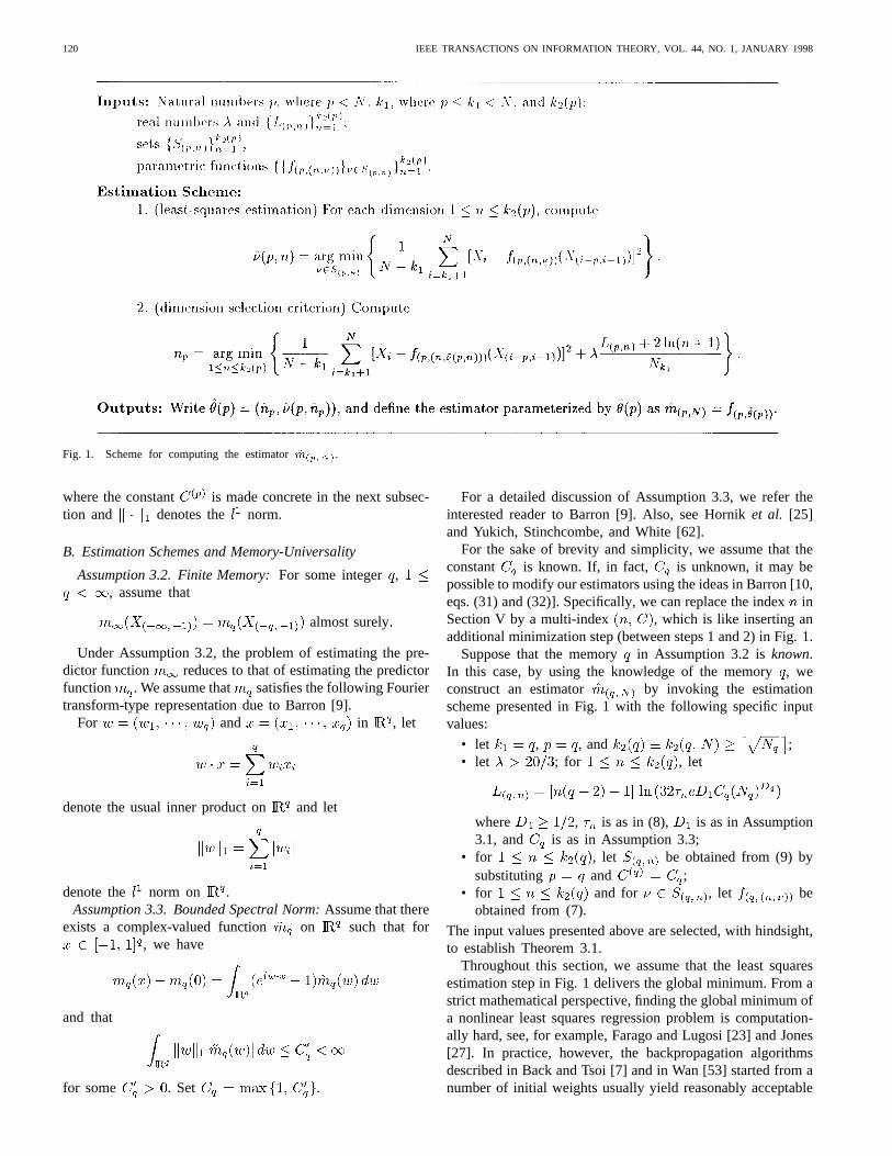
Fig. 1. Scheme for computing the estimatorm(p;N).

where the constant is made concrete in the next subsec-tion and denotes the norm.

B. Estimation Schemes and Memory-Universality

Assumption 3.2. Finite Memory:For some integer ,, assume that

almost surely

Under Assumption 3.2, the problem of estimating the pre-dictor function reduces to that of estimating the predictorfunction . We assume that satisfies the following Fouriertransform-type representation due to Barron [9].

For and in , let

denote the usual inner product on and let

denote the norm on .Assumption 3.3. Bounded Spectral Norm:Assume that there

exists a complex-valued function on such that for, we have

and that

for some . Set .

For a detailed discussion of Assumption 3.3, we refer theinterested reader to Barron [9]. Also, see Horniket al. [25]and Yukich, Stinchcombe, and White [62].

For the sake of brevity and simplicity, we assume that theconstant is known. If, in fact, is unknown, it may bepossible to modify our estimators using the ideas in Barron [10,eqs. (31) and (32)]. Specifically, we can replace the indexinSection V by a multi-index , which is like inserting anadditional minimization step (between steps 1 and 2) in Fig. 1.

Suppose that the memory in Assumption 3.2 isknown.In this case, by using the knowledge of the memory, weconstruct an estimator by invoking the estimationscheme presented in Fig. 1 with the following specific inputvalues:

• let , , and ;• let ; for , let

where , is as in (8), is as in Assumption3.1, and is as in Assumption 3.3;

• for , let be obtained from (9) bysubstituting and ;

• for and for , let beobtained from (7).

The input values presented above are selected, with hindsight,to establish Theorem 3.1.

Throughout this section, we assume that the least squaresestimation step in Fig. 1 delivers the global minimum. From astrict mathematical perspective, finding the global minimum ofa nonlinear least squares regression problem is computation-ally hard, see, for example, Farago and Lugosi [23] and Jones[27]. In practice, however, the backpropagation algorithmsdescribed in Back and Tsoi [7] and in Wan [53] started from anumber of initial weights usually yield reasonably acceptable


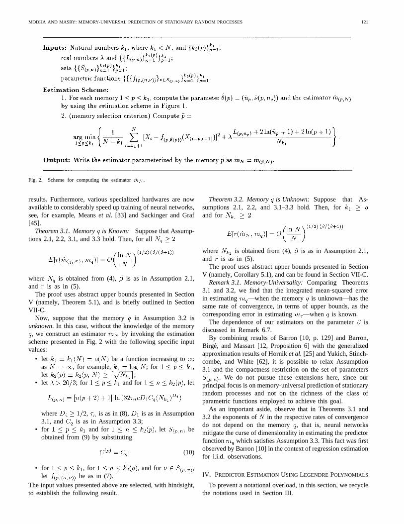
Fig. 2. Scheme for computing the estimatormN .

results. Furthermore, various specialized hardwares are nowavailable to considerably speed up training of neural networks,see, for example, Meanset al. [33] and Sackinger and Graf[45].

Theorem 3.1. Memory is Known: Suppose that Assump-tions 2.1, 2.2, 3.1, and 3.3 hold. Then, for all

where is obtained from (4), is as in Assumption 2.1,and is as in (5).

The proof uses abstract upper bounds presented in SectionV (namely, Theorem 5.1), and is briefly outlined in SectionVII-C.

Now, suppose that the memory in Assumption 3.2 isunknown. In this case, without the knowledge of the memory, we construct an estimator by invoking the estimation

scheme presented in Fig. 2 with the following specific inputvalues:

• let be a function increasing toas , for example, ; for ,let ;

• let ; for and for , let

where , is as in (8), is as in Assumption3.1, and is as in Assumption 3.3;

• for and for , let beobtained from (9) by substituting

(10)

• for , for , and for ,let be as in (7).

The input values presented above are selected, with hindsight,to establish the following result.

Theorem 3.2. Memory is Unknown: Suppose that As-sumptions 2.1, 2.2, and 3.1–3.3 hold. Then, forand for


The proof uses abstract upper bounds presented in SectionV (namely, Corollary 5.1), and can be found in Section VII-C.

Remark 3.1. Memory-Universality:Comparing Theorems3.1 and 3.2, we find that the integrated mean-squared errorin estimating —when the memory is unknown—has thesame rate of convergence, in terms of upper bounds, as thecorresponding error in estimating —when is known.

The dependence of our estimators on the parameterisdiscussed in Remark 6.7.

By combining results of Barron [10, p. 129] and Barron,Birge, and Massart [12, Proposition 6] with the generalizedapproximation results of Horniket al. [25] and Yukich, Stinch-combe, and White [62], it is possible to relax Assumption3.1 and the compactness restriction on the set of parameters

. We do not pursue these extensions here, since ourprincipal focus is on memory-universal prediction of stationaryrandom processes and not on the richness of the class ofparametric functions employed to achieve this goal.

As an important aside, observe that in Theorems 3.1 and3.2 the exponents of in the respective rates of convergencedo not depend on the memory, that is, neural networksmitigate the curse of dimensionality in estimating the predictorfunction which satisfies Assumption 3.3. This fact was firstobserved by Barron [10] in the context of regression estimationfor i.i.d. observations.

IV. PREDICTORESTIMATION USING LEGENDREPOLYNOMIALS

To prevent a notational overload, in this section, we recyclethe notations used in Section III.


A. Legendre Polynomials

Let denote the normalized Legendre polynomi-als [49] which are orthogonal with respect to the Lebesguemeasure on , where is a polynomial of degree

. Let IN . For , we now define atensor product Legendre polynomial on , indexed bya multi-integer IN , as

(11)

where .Fix and . Let

(12)

Let IN and IN .We adopt the convention that the inequalities between multi-integers are to be interpreted component-wise. For ,let . Let represent a -dimensional parameter vector. Define a tensor product Le-gendre polynomial with dimension (or the largest coordinate-wise degree) and memory (or time delays) param-eterized by as

(13)

where

and is as in (11). We restrict attention to a compactsubset of , namely,

(14)

B. Estimation Schemes and Memory-Universality

In this subsection, we suppose that Assumption 3.2 holds,that is, the predictor function has a finite memory .We assume that satisfies the following differentiabilitycondition.

Assumption 4.1 Differentiability:For some unknownsmoothness order , assume that all partial derivativesof total order of the function exist, are measurable,and are square-integrable.

In this section, we approximate the predictor functionusing Legendre polynomials. We note that various other fam-ilies of approximants such as trigonometric series, splines,neural networks, or wavelets would suffice as well.

In the sequel, we need the following technical condition.Assumption 4.2:Assume that the marginal distribution of

, namely, , has a uniformly bounded probabilitydensity.

Suppose that the memory in Assumption 3.2 isknown.In this case, by using the knowledge of the memory, weconstruct an estimator by invoking the estimation

scheme presented in Fig. 1 (see Section III) with the followingspecific input values:

• let , , and ;• let ; for , let

where ;• for , let be obtained from (14);• for and for , let be

obtained from (13).

Note that the estimator makes no use of the smooth-ness order . The input values presented above are selected,with hindsight, to establish the following result.

Theorem 4.1. Memory is Known: Suppose that Assump-tions 2.1, 2.2, 4.1, and 4.2 hold. Then, for all


The proof uses abstract upper bounds presented in SectionV (namely, Theorem 5.1), and is briefly outlined in SectionVII-D.

Now, suppose that the memory in Assumption 3.2 isunknown. In this case, without the knowledge of the memory, we construct an estimator by invoking the estimation

scheme presented in Fig. 2 (see Section III) with the followingspecific input values:

• let be a function increasing toas , for example, ; for ,let ;

• let ; for and for , let

where ;• for and for , be as

in (14);• for , for , and for ,

let be as in (13).

Note that the estimator makes no use of the smoothnessorder . The input values presented above are selected, withhindsight, to establish the following result.

Theorem 4.2. Memory Is Unknown: Suppose that As-sumptions 2.1, 2.2, 3.2, 4.1, and 4.2 hold. Then, forand for


The proof uses abstract upper bounds presented in Sec-tion V (namely Corollary 5.1), and can be found in SectionVII-D.

Observe that Remark 3.1, when properly translated, contin-ues to hold in the current context as well. The dependence ofour estimators on the parameteris discussed in Remark 6.7.


By modifying our estimators using the ideas in Barron [11],it is possible to eliminate the logarithmic factor in Theorems4.1 and 4.2. However, for the sake of simplicity, and also sincethe resulting estimators are computationally more expensive,we do not pursue that direction here.

C. Consistent Estimation of

In this subsection, unlike the previous one, we do notassume that the predictor function has a finite memory.Nonetheless, we continue to estimate the predictor function

using the estimator constructed in the previoussubsection. To establish consistency of , we require thefollowing technical condition.

Assumption 4.3:For each memory , assumethat the marginal distribution of , namely, , has auniformly bounded probability density.

Theorem 4.3. Consistency:Suppose that Assumptions 2.1,2.2, and 4.3 hold. Then,

(15)

where is as in (5).The proof uses abstract upper bounds presented in Sec-

tion V (namely, Theorem 5.2), and can be found in SectionVII-D.

To obtain a rate of convergence for inTheorem 4.3, we first need to obtain a rate of convergence forthe “approximation error” under Assumption 2.1.To the best of our knowledge, no such results are currentlyknown.

Since the same estimator is considered in Theorems4.2 and 4.3, we have that if the predictor function hasa finite memory, then delivers memory-universality, andeven if the predictor function does not have a finite memory,

delivers consistency. Also, observe that in Theorem 4.3no smoothness assumptions are imposed on the predictorfunction .

V. ABSTRACT ESTIMATION FRAMEWORK

In this section, given a sequence of abstract parametricfamilies of functions, we propose an estimator, say, for thepredictor function , and upper-bound the integrated mean-squared error of the estimator in terms of certain indices ofresolvability. The benefit of abstraction is that we are able tocapture the statistics behind the proposed estimation scheme inthe most general case, in a clean, economical fashion, withoutworrying about the cumbersome details of the specific casesof interest.

Throughout this section, fix the number of observations.

A. Parameter Spaces and Complexities

The development in this subsection closely follows that in[34, Subsec. 3.A].

Throughout this subsection, fix a memory . Foreach integer , let denote a model dimension (forexample, see (6) and (12)), and let denote a compactsubset of . The set will serve as a collection of

parameters associated with the model dimension (forexample, see (9) and (14)). By introducing a prior density onthe set as in Barron [10, p. 129], it is possible to relaxthe compactness assumption.

For every , let denote a real-valuedfunction on parameterized by (for example,see (7) and (13)). The following condition is required to beable to invoke the Craig–Bernstein inequalities in Lemma 7.1.

Assumption 5.1:For each integer and for every, assume that takes values in .

Owing to the “clip” function in (7) and (13), Assump-tion 5.1 is satisfied for both neural networks and Legendrepolynomials.

Let denote a metric on . For , letdenote an -net of the set ; in other

words, for every there exists asuch that . Assume that .Let be such that

(16)

where and denotes the cardinality operator.Example 5.1. Neural Networks:Let notations be as in Sec-

tion III. Let denote a metric on defined as inBarron [10, eq. (19)], but by replacingthere by . It followsfrom [10, Lemma 2] by using (8) that for every andfor every , there exists a -net of ,namely, , such that

(17)

Example 5.2. Legendre Polynomials:Let notations be asin Section IV. Let be simply the metric on .The hypersphere is contained in the hypercube

, which has volume .Furthermore, the set can be coveredby (small) hypercubes (with respect to the metric ) withside length . Since by assumption , thereexists a -net of , namely, , such that

(18)

Assumption 5.2:For every , there exists a strictlyincreasing function (in) such thatfor all and for all andwith we have

Assumption 5.2 implies that the function is invert-ible; let denote the inverse. Observe that the inverse

is defined for all andtakes values in the range .

Assumption 5.2 says that the class of parametric functions

can be covered in the supremum norm over by afinite class of functions. In other words, we limit attention to


classes of parametric functions where upper bounds on thesup-norm covering numbers of are available; also,see [8], [32], and [34]. This class is sufficient to demonstrateour main contribution on memory-universal prediction ofstationary random processes. We note in passing that moregeneral classes of parametric functions have been considered,for instance, by Barron, Birge, and Massart [12], Lugosi andNobel [28], and Lugosi and Zeger [29], [30] in the context offunction estimation in an i.i.d. setting.

Example 5.1 (continued):It follows from [10, Lemma 1],by invoking Assumption 2.2 and Part b) of Assumption 3.1,that Assumption 5.2 holds with . Forall , the inverse of canbe written as

(19)

Example 5.2 (continued):Letand let

be such that . The following calcula-tion shows that Assumption 5.2 holds with

.

where follows from (13). For all

the inverse of can be written as

(20)

Let denote a natural number (for example,for neural networks and for

Legendre polynomials). Let denote a collectionof parameters of different dimensions, with the maximumdimension less than or equal to , such that each of theparameters comes packaged with the index of its dimension;formally, we write

(21)

It follows from (21) that every must be ofthe form for some and for some

; then, define

(22)

and for every define the “descriptioncomplexity” of the parameter as

(23)

where is as in Assumption 5.2 and

is obtained from (16) by substituting .

B. An Abstract Scheme for Computing

In this subsection, as a building block for the estimationscheme presented in the next subsection, we outline a schemeto construct the estimator . The estimation schemepresented in this subsection is conceptually the same as thatpresented in [34, eqs. (25), (26)], but is different in details.

For any natural number, where , for any naturalnumber , where , for any natural number ,for any real number , where2

and for any real number, write

(24)

where is as in (21), is as in (22),is as in (23), and is obtained from (4). Now, define theestimator parameterized by as

(25)

We may now interpret the estimation scheme presented inFig. 1 (see Section III) as a computationally convenient ver-sion of (24) and (25), which are analytically more convenient.For the sake of simplicity, in Fig. 1, we write instead ofthe complete expression and we implicitlyset .

Define the -index of resolvabilitycorresponding to theestimator as

(26)

where is as in (21), is as in (23), isobtained from (4), and is obtained from (5) bysubstituting and .

Remark 5.1:The index of resolvability was first introducedby Barron and Cover [13] in the context of density estimationfor i.i.d. observations, and by Barron [8] in the context ofregression estimation for i.i.d. observations.

2If we let 0 < � � $(p; n)(1), then$�1(p; n)(�) is well defined. Thus if

we let

0 < � � min1�n�k (p)

$(p; n)(1)

then$�1(p; n)(�) is well defined for each1 � n � k2(p).


Theorem 5.1:Let be a natural number such that .Set . Suppose that Assumptions 2.1 and 2.2 hold,and that Assumptions 5.1 and 5.2 hold. Then, for all naturalnumbers , for all real numbers

for all , and for all

(27)

where , , ,and .

The proof is briefly outlined in Section VII-B.

C. An Abstract Scheme for Computing

For any natural number , where , for any naturalnumbers , for any real number , where

and for any real number, write

(28)

where is as in (24) and is obtained from(23) by substituting . Roughly speaking, the adaptivememory is an estimator of the memory of the underlyingpredictor function . We now write the estimator as

(29)

We may now interpret the estimation scheme presented inFig. 2 (see Section III) as a computationally convenient ver-sion of (28) and (29), which are analytically more convenient.For the sake of simplicity, in Fig. 2, we write in-stead of the complete expression and we

implicitly set .Theorem 5.2:Let be a natural number such that. Suppose that Assumptions 2.1 and 2.2 hold, and that

Assumptions 5.1 and 5.2 hold for each . Then,for all natural numbers , for all real numbers

for all , for all , and for all

where , , ,, and is as in (26).

The proof can be found in Section VII-B.

Remark 5.2:Observe from the proofs of Theorems 5.1 and5.2 that the bounds stated in the theorems continue to holdeven when the parameters, , and are functions of

.Remark 5.3:Observe that the index of resolvability (which

consists of an approximation error term and an estimation errorterm) in Theorems 5.1 and 5.2 is multiplied by a constant

. This implies that, for each fixed , the upper boundsestablished in Theorems 5.1 and 5.2 may not be the bestpossible—in the sense of constant multipliers. In a conceptlearning (or pattern recognition) setting, Lugosi and Zeger[30] avoid the problem of constant multipliers larger than

by using a Vapnik–Chervonenkis framework. However, ina mean-squared regression setting, a direct application oftheir method of analysis leads to a slower overall rate ofconvergence which is less desirable.

Corollary 5.1: Suppose all hypotheses of Theorem 5.2hold. In addition, suppose that Assumption 3.2 holds and that

. Then

(30)

where is obtained from (26) by substituting.

Proof: The corollary follows by applying Theorem 5.2with (since ) and (since Assumption3.2 holds).

VI. DISCUSSION

Remark 6.1. Related Works:We now discuss the relevantliterature to establish a broader context for our results.

• Suppose that the process is binary-valued.In this case, estimating the predictor function isessentially the same as estimating the corresponding con-ditional distribution of given the entire infinite history

. The latter problem, owing to its applicationsin data compression, has received wide attention, forexample, see Algoet [2], Cover [18], Rissanen [37], [38],and Ryabko [43], [44]. Our work fundamentally differsfrom the existing body of work for binary-valued pro-cesses in that, for binary-valued processes each elementof the sequence is finitely parameterized, whilefor real-valued processes considered here the elements ofthe sequence are not finitely parameterized.

• Suppose that the process is real-valued, sta-tionary, Gaussian ARMA. In this case, estimation of thepredictor function has been widely studied, for ex-ample, see Akaike [1], Bhansali [14], and Rissanen [39].Our work fundamentally differs from the existing body ofwork for Gaussian ARMA processes, in that, for GaussianARMA processes each element of the sequenceis linear (in the observations) and finitely parameterized,while for stationary random processes considered here theelements of the sequence are neither linear nor finitelyparameterized.


• Recently, supposing that the process is real-valued, stationary, and ergodic, Algoet [2], [3], Morvai,Yakowitz, and Gyorfi [36], and Morvai, Yakowitz, andAlgoet [35] proposed several nonparametric estimatorsof the predictor function , and established universalconsistency of their estimators. This is distinct frommemory-universality—which is the main focus of thispaper.

• Recently, supposing that the process is real-valued, stationary mixingale, Sin and White [47] proposedmodel selection criteria with the goal of selecting thebest (in the sense of the smallest approximation error)of two abstract parametric models of the predictor func-tion3 , and exemplified their model selection criteriafor ARMAX-GARCH and STAR models. Although weconsider a smaller class of processes, our estimatorsare applicable to sequences of parametric families offunctions, minimize the overall statistical risk (that is,approximation error estimation error), and are memory-universal and consistent.

• Supposing that the process is real-valued,exponentially strongly mixing, and that the predictorfunction has a finite memory (see (2)), Auestad andTjøstheim [5], [6] (also see Tjøstheim [50]) and Chengand Tong [17] proposed two-step schemes (based on thenonparametric kernel approach) to estimate the predictorfunction , without the knowledge of the memory. However, no analytical results are yet available for

the estimators considered by Auestad and Tjøstheim,and although Cheng and Tong established the orderconsistency of their scheme, they did not establish, likewe do, rates of convergence for the statistical risk.

Remark 6.2. General Regression Estimation Problem:Although so far we confined our attention to the simple andintuitively appealing problem of one-step-ahead predictionof stationary random processes, our results easily extend toa larger class of estimation problems as shown below. Let

be a stationary random process such thattakes values in and takes values in . Letbe a measurable function such that . For

and for , define the regression function as

Given a sequence of observations , we are in-terested in estimating the regression function . If wesuppose that the process satisfies Assumption2.1, suppose that takes values in , and replacein Figs. 1 and 2 (equivalently, in (24) and (28)) by ,then we can use the resulting as our estimator of .Furthermore, all our results in Sections III–V continue to hold.Also, observe that by selecting various values for the function

, we can obtain a number of interesting special cases asfollows.

3Note that although, for the sake of coherence, we have paraphrased thecontribution of the literature dealing with Gaussian ARMA processes [1], [14],[39] and that of Sin and White [47] as estimating the predictor functionm1,they did not phrase their work as such.

• ( -Step-Ahead Prediction) If we set ,and assume that takes values in , then we canestimate .

• (Conditional Moments Estimation) If we set ,where , and assume that takes values in ,then we can estimate .

• (Conditional Distribution Estimation) If we set, where is a fixed real number, then we can

estimate .

Remark 6.3. Consistent Estimation of Using Neu-ral Networks: Observe that we did not establish a resultanalogous to Theorem 4.3 for the estimator based onneural networks. Now consider the following relatively strongcondition.

Assumption 6.1:For each , assume that there existsa complex-valued function on such that for

, we have

and that

for some known . Set . Supposethat Assumptions 2.1, 2.2, and 6.1 hold, and let be as inSection III, where we replace (10) by . Then, it ispossible to show, by proceeding as in the proof of Theorem4.3, that

as

where convergence is in the sense of integrated mean-squarederror. However, owing to the stringent nature of Assumption6.1, such a result appears unappealing.

Remark 6.4. Compact Parameter Spaces:Throughout thispaper, we restricted attention to sequences of parametricfamilies with compact parameter spaces. This assumption issufficient to treat the examples presented here. However, if thepredictor function is such that one must use a sequenceof parametric families with noncompact parameter spaces toobtain the best bounds on the approximation error, then thecurrent framework may prove wanting. It may be possible toextend our framework to more general sequences of parametricfamilies along the directions considered, for instance, byBarron, Birge, and Massart [12], Lugosi and Nobel [28], andLugosi and Zeger [29], [30].

Remark 6.5. Order Consistency and Price of Memory-Universality: In Theorems 3.1 and 3.2 (see also Theorems4.1 and 4.2), we established the memory-universality of theestimator . However, it should be noted that is,roughly speaking, times more expensive tocompute than the corresponding estimator that doesknow the memory . It is currently unknown whether theadaptive memory converges to in some sense; nevertheless,

does converge to the predictor function .


Remark 6.6. Conditional Density and Conditional Quan-tiles: Assuming that the predictor function has a finitememory, we formulated memory-universal and consistent esti-mators for . It may also be possible to apply our estimationmethodology and proof techniques along with the results ofBarron and Cover [13], Barron [8], Barron, Birge, and Massart[12], and White [56] to establish memory-universality andconsistency of suitable estimators of the conditional densityand of various conditional quantiles of given .

Remark 6.7. Dependence of our Estimators on: Thecomplexity term in (24) and (28) is motivated solely bythe statistical risk bounds we are able to obtain and not byother information-theoretic or Bayesian considerations. As aconsequence, the complexity term depends explicitly on theparameter in Assumption 2.1. In practice, one may set ,since important classes of processes satisfy Assumption 2.1with that value [59]. Note, however, that if the true underlying

is larger than the value of used in our estimators, thenthe resulting estimators will deliver a slower rate than thatobtainable with the knowledge of the true. On the otherhand, if the value of used in our estimators is larger than thetrue underlying , then we are unable to quantify the statisticalperformance of the resulting estimators. Unfortunately, unlikethe parameters “smoothness,” “norm,” model dimension, ormodel memory, it does not appear possible to selectin adata-driven fashion using complexity regularization. Further-more, we are currently unaware of any algorithm for testingthe exponentially strongly mixing condition.

Remark 6.8. Comparison with Nonparametric Prediction:We have from Theorem 3.1 that

(31)

Now, suppose that the strong mixing coefficient decays alge-braically, and that the predictor function has continuousand bounded partial derivatives of total order. Letdenote a nonparametric kernel estimator [15], [40], [41] whichuses a kernel of order, then it is known that with an optimaldeterministic choice of the corresponding bandwidth parameter

(32)Directly comparing (31) and (32), we find that rate of con-vergence for our estimator decreases by the factor

. However, the above comparison may be inherentlyunfair, since our estimator selects the model dimen-sion in a data-driven fashion whereas the kernel estimator

does not select its bandwidth parameter in a data-driven fashion. A fair comparison would involve a kernelestimator which selects its bandwidth parameter in a data-driven fashion (using, say, cross-validation). Unfortunately,to our knowledge, obtaining rates of convergence results forkernel estimators with data-driven bandwidth selection, inthe context of dependent observations, is currently an openproblem.

VII. D ERIVATIONS

A. A Sequence of Craig–Bernstein Inequalities

To furnish the key technical tool required in the proof ofTheorem 5.2, we now extend the Craig–Bernstein inequalityin [34, Theorem 4.3]. Specifically, in proof of Theorem 5.2,we need to analyze empirical means of the form

(33)

where and is a Borel measurable functionfrom to , using a Craig–Bernstein-type inequality. Thefollowing lemma supplies the needed sequence of inequalitiesfor each (the Craig–Bernstein inequality in [34, Theorem4.3] corresponds to the case ).

Lemma 7.1. ( )-Craig–Bernstein Inequality: Supposethat Assumption 2.1 holds. Let integers and be such that

. Let be a Borel measurablefunction. For each , let .Assume that a.s. and that . Let beas in (4). Then, for all , for all , and for all

Proof: The proof closely follows the proof of [34, The-orem 4.3]; here we merely point out the main points ofdeparture. Since in our case , the sigma-algebras of events

and

in item b) in the proof of [34, Lemma 4.2], are now measurablewith respect to

and , respectively. Thus the dis-tance between the two sigma-algebras now becomes

Consequently, in [34, Lemma 4.2], we now must apply themixing inequality in Hall and Heyde [24, Theorem A.5] with

instead of . In other words, throughout [34,Lemma 4.2], we should replace by , and shouldreplace the constraint by . Also, throughout [34,Theorem 4.3], we replace by and replace by

. Finally, note that the “number of blocks” in [34, eq.(44)] now becomes


and hence the “block size” or the effective number of obser-vations in [34, eq. (39)] now becomes

which is exactly the prescribed value in (4).

B. Proofs of Theorems 5.1 and 5.2

To establish a perspective for the method of analysis usedin establishing Theorems 5.1 and 5.2, we recall a techniqueused by Barron [8]. Let be a sequence ofi.i.d. random variables. Define the regression function by

. Given observations ,Barron proposed a certain estimator, say, of based on anabstract sequence of parametric models, and established upperbounds on the integrated mean-squared error byanalyzing

(34)

for each parameter with dimension , using theclassical Craig–Bernstein inequality. In [34], assuming that theprocess is exponentially strongly mixing, weanalyzed (34) using the Craig–Bernstein inequality establishedthere.

Proof of Theorem 5.1:Motivated by the above discus-sion, we can upper-bound the integrated mean-squared error

by analyzing

(35)

for each parameter with a fixed memory anddimension . With this insight, the theoremfollows by proceeding essentially as in [34, Proof of Theorem3.1] but by using the -Craig–Bernstein inequality inLemma 7.1.

Proof of Theorem 5.2:Here, we seek upper bounds onthe integrated mean-squared error . To moti-vate our method of proof, we first explain two approaches thatdo not work. As a first try, motivated by (34) and (35), onemay attempt to directly analyze

(36)

for each parameter with memory anddimension . But, since each term in thesecond sum in (36) depends on an infinite past, no meaningfulCraig–Bernstein inequalities appear possible for the empiricalmean (36).

As a second try, one may attempt to analyze (35) for eachparameter with memory and dimension

by using the -Craig–Bernsteininequality in Lemma 7.1. This would lead to the desired upperbounds on , if we select the memory as

(37)

where and are as in (28). Sincein (37) depends on the predictor

function (see (35)), implementing (37) would require theknowledge of the sequence of predictors —whichis not available.

As a key technical insight, here, we analyze the empiricalprocess

(38)

for each parameter with memory and dimension, using the -Craig–Bernstein

inequality, and, consequently, obtain upper bounds on. Note that the second sum in (38) has a

finite memory and does not depend on. Next, by simpleprobabilistic manipulations, we observe that (see Lemma 7.6)

(39)

Equation (39) combined with the upper bounds onleads to the desired upper bounds on

. In other words, instead of estimating ,we estimate for a growing memory (as ).Then, by virtue of the -martingale convergence theorem,we are automatically doing a good job in estimating .

To make the lengths of various equations manageable,throughout this proof, we write , ,

, , and .Let be a natural number such that . For each

fixed , for each fixed , and for eachfixed , write

(40)

(41)

We now proceed with a series of lemmas.Lemma 7.2:Let and be natural numbers such that

. Suppose that Assumptions 5.1, 5.2, 2.1, and2.2 hold. Then, for all


for all , for all , for all , andfor all

Proof: For , write

(42)

where is as in (40), and observe thatare identically distributed. By invoking Assumptions 5.1 and2.2, and by proceeding as in [8], we have that

and

Also, it follows from (41) and (42) that

(43)

Since Assumption 2.1 holds and since areidentically distributed, the lemma follows by applying the

-Craig–Bernstein inequality in Lemma 7.1 to (43)(with , , and

) just as the -Craig–Bernstein inequality wasapplied in [34, Lemma 3.1] to (29) there.

Lemma 7.3: Let be a natural number such that .Suppose that Assumptions 5.1 and 5.2 hold for each

, and that Assumptions 2.1 and 2.2 hold. Then, forall , for all , for all , and for all

(44)

Proof: Observe that and that. Thus, to establish (44), one can first establish

(45)

for each fixed . Since the sets aredisjoint, we can then pass from (45) to (44) using a unionbound argument. However, we can establish (45) by invokingLemma 7.2 and by proceeding essentially as in [34, Lemma3.2]. We omit the details.

Let be the element of the set , which attainsthe -index of resolvability in (26); formally,we write

(46)

Lemma 7.4:Suppose all hypotheses of Lemma 7.3 hold.Then, for each , we have

Proof: Recall the definition of in (40) and (41).

(47)

where follows from (28); and follows from (24). Thelemma now follows from Lemma 7.3 and (47).

Lemma 7.5:Let and be natural numbers such that. Suppose that Assumptions 5.1, 2.1, and 2.2 hold.

Then, for all , for all , and for all

Proof: Let be obtained from (40) by substi-tuting . For , write

The lemma follows by applying the -Craig–Bernsteininequality in Lemma 7.1 to the sum

with , , and and by simplifyingas in [34, Lemma 3.1].


Lemma 7.6: Let and let, then

Proof:

Lemma 7.7: Suppose all hypotheses of Theorem 5.2 hold.Then, for each , we have

Proof: Combining Lemmas 7.4 and 7.5, we have

(48)

Applying Lemma 7.6 with , , and, we have

(49)

Now, ignoring the term

we have from (26), (46), (48), and (49) that

By writing

and for setting , we have that

(50)

It is easy to see that , and hence . Thelemma now follows from (50) and [34, Lemma A.6].

The following upper bounds complete the proof of Theo-rem 5.2.

where follows by applying Lemma 7.6 (with ,, , and ) on a realization-by-realization

basis; follows from Lemma 7.7 for each ; andfollows by applying Lemma 7.6 (with , ,

, and ) and since .

C. Proofs of Theorems 3.1 and 3.2

First, in Lemma 7.8 below, we establish an upper bound on acertain index of resolvability. We will then establish Theorem3.1 (respectively, Theorem 3.2) by combining Lemma 7.8 andTheorem 5.1 (respectively, Corollary 5.1).

Lemma 7.8 A Bound on Index of Resolvability:Supposethat Assumptions 2.2 and 3.3 hold. Let be a natural numbersuch that . Then, for all , for all

, where , and for all , we have

where is obtained from (26) and isobtained from (4).

Proof: The proof follows by proceeding as in [34,Lemma 2.2]. We omit the details.

Proof of Theorem 3.1:Theorem 3.1 follows by combin-ing Theorem 5.1 (for ) and Lemma 7.8 (for ) inthe manner of Theorem 3.2; we omit the details.

Proof of Theorem 3.2:It follows from our hypothesesthat Assumptions 2.1, 2.2, 3.2 hold, and from Example 5.1that Assumptions 5.1 and 5.2 hold for all .Consequently, all hypotheses of Corollary 5.1 hold, and wehave for all , for all , for

, and for all

where follows by applying Lemma 7.8 with ,, and , where ;

and follows if we let , and from (4) by simplealgebraic manipulations since .


D. Proofs of Theorems 4.1–4.3

First, in Lemma 7.9 below, we establish an upper bound on acertain index of resolvability. We will then establish Theorem4.1 (respectively, Theorem 4.2) by combining Lemma 7.9 andTheorem 5.1 (respectively, Corollary 5.1).

Lemma 7.9 A Bound on the Index of Resolvability:Supposethat Assumptions 2.2, 4.1, and 4.2 hold. Let be a naturalnumber such that . Then, for all ,

, where , and for all , we have

where is obtained from (26) and isobtained from (4).

Proof:

where follows from (21), (23), and (26), where isobtained from (14), is obtained from (13),is obtained from (18), and is obtained from (20); itfollows from Assumption 4.2 that there exists a finite uniform

bound on the probability density of the marginaldistribution . Hence

IN(51)

where

and the polynomial is obtained from (11). Now, ob-taining upper bounds on the tail term in (51) is a standardexercise in multivariate approximation theory. Specifically,under Assumption 4.1, it can be shown that

IN

see, for example, Canuto and Quarteroni [16] or Sheu [46,Theorem 4.2]. Finally, set ; follows from(18) by setting , and also since

; follows by setting for some; since , follows by setting

and ; follows by settingand by setting ;

g) follows by setting ; followsby setting , which takes valuesin the set for .

Proof of Theorem 4.1:Theorem 4.1 follows by combin-ing Theorem 5.1 (for ) and Lemma 7.9 (for ) inthe manner of Theorem 4.2; we omit the details.

Proof of Theorem 4.2:It follows from our hypothesesthat Assumptions 2.1, 2.2, and 3.2 hold, and from Example5.1 that Assumptions 5.1 and 5.2 hold for all .Consequently, all hypotheses of Corollary 5.1 hold, and wehave for all , for all , for ,and for all

where follows by applying Lemma 7.9 with ,, and , where ;

and follows if we let , and from (4) by simplealgebraic manipulations since .


Proof of Theorem 4.3:Choose a small . We knowby the martingale convergence theorem thatmonotonically decreases toas . Hence, there existsan integer such that

(52)

where constant is as in the hypothesis of Theorem 5.2.For IN , define

(53)

where the polynomial is obtained from (11). Write

(54)

where IN and IN .It follows from Parseval’s identity that

IN

(55)

where the last inequality follows since the range ofis . Since the polynomial system IN iscomplete and orthonormal for the space of measurable, square-integrable (with respect to the Lebesgue measure) functions on

, there exists a dimension such that

(56)

where IN and denotes the uniformbound, which is finite by Assumption 4.3, on the probabilitydensity of the marginal distribution . Since clip iscontinuous, we have from (13) that

(57)

We have from Assumption 4.3, (56), and (57) that

(58)

The following sequence of upper bounds essentially com-pletes the proof.

(59)

where follows by invoking Theorem 5.2 for , forall , for all , for all , forall , and for all large such that ;follows from (52) and by setting , where

; follows from (21), (23), and (26), where isobtained from (14), is obtained from (13),is obtained from (18), and is obtained from (20);holds for all large such that and ;

follows since we have from (14), (54), and (55), that; follows from (58) and from (18) and (20);

and follows by simple algebraic manipulations.Since we may choose as small as desired, and since

(since ), the theorem follows from(59).

ACKNOWLEDGMENT

The authors wish to thank S. Altekar, R. Hecht-Nielsen, H.Mhaskar, J. Rissanen, and H. White for valuable discussions.

REFERENCES

[1] H. Akaike, “A new look at the statistical model identification,”IEEETrans. Automat. Contr., vol. AC-19, pp. 716–723, 1974.

[2] P. H. Algoet, “Universal schemes for prediction, gambling, and portfolioselection,”Ann. Probab., vol. 20, no. 2, pp. 901–941, 1992. Correction:ibid., vol. 23, pp. 474–478, 1995.

[3] , “The strong law of large numbers for sequential decisions underuncertainty,” IEEE Trans. Inform. Theory, vol. 40, pp. 609–633, May1994.

[4] K. B. Athreya and S. G. Pantula, “Mixing properties of Harris chainsand autoregressive processes,”J. Appl. Probab., vol. 23, pp. 880–892,1986.

[5] B. Auestad and D. Tjøstheim, “Identification of nonlinear time series:First order characterization and order determination,”Biometrika, vol.77, no. 4, pp. 669–687, 1990.


[6] , “Functional identification in nonlinear time series,” inPro-ceedings NATO Advanced Study Institute on Nonparametric FunctionalEstimation, G. Roussas, Ed. Dordrecht, The Netherlands: Kluwer,1991.

[7] A. D. Back and A. C. Tsoi, “FIR and IIR synapses, a new neuralnetwork architecture for time series modeling,”Neural Comput., vol.3, pp. 375–385, 1991.

[8] A. R. Barron, “Complexity regularization,” inProceedings NATO Ad-vanced Study Institute on Nonparametric Functional Estimation,G.Roussas, Ed. Dordrecht, The Netherlands: Kluwer, 1991, pp. 561–576.

[9] , “Universal approximation bounds for superpositions of a sig-moidal function,” IEEE Trans. Inform. Theory, vol. 39, pp. 930–945,May 1993.

[10] , “Approximation and estimation bounds for artificial neuralnetworks,”Mach. Learn., vol. 14, pp. 115–133, 1994.

[11] , “Asymptotically optimal model selection and neural nets,” inProc. 1994 IEEE-IMS Workshop on Information Theory and Statistics.New York: IEEE Press, Oct. 1994, p. 35.

[12] A. R. Barron, L. Birge, and P. Massart, “Risk bounds for model selectionvia penalization,” 1995, preprint.

[13] A. R. Barron and T. M. Cover, “Minimum complexity density esti-mation,” IEEE Trans. Inform. Theory, vol. 37, pp. 1034–1054, July1991.

[14] R. J. Bhansali, “Order selection for linear time series models: A review,”in Developments in Time Series Analysis: In Honour of M. B. Priestley,T. Subba Rao, Ed. New York: Chapman and Hall, 1993, pp. 50–66.

[15] D. Bosq,Nonparametric Statistics for Stochastics Processes: Estimationand Prediction. New York: Springer-Verlag, 1996.

[16] C. Canuto and A. Quarteroni, “Approximation results for orthogonalpolynomials in Sobolev spaces,”Math. of Computation,vol. 38, pp.67–86, 1982.

[17] B. Cheng and H. Tong, “On consistent nonparametric order determina-tion and chaos,”J. Roy. Statist. Soc., B, vol. 54, no. 2, pp. 427–449,1992.

[18] T. M. Cover, “Open problems in information theory,” inProc. 1975IEEE-USSR Joint Workshop on Information Theory,(Moscow, USSR,Dec. 15–19, 1975). New York: IEEE Press, 1975.

[19] Y. A. Davydov, “Mixing conditions for Markov chains,”Theory Probab.Applications, vol. XVIII, no. 2, pp. 312–328, 1973.

[20] L. Devroye, L. Gyorfi, and G. Lugosi,A Probabilistic Theory of PatternRecognition. New York: Springer-Verlag, 1996.

[21] P. Doukhan,Mixing: Properties and Examples.New York: Springer-Verlag, 1994.

[22] R. Durrett, Probability: Theory and Examples.Pacific Grove, CA:Wadsworth & Brooks, 1991.

[23] A. Farago and G. Lugosi, “Strong universal consistency of neural net-work classifiers,”IEEE Trans. Inform. Theory, vol. 39, pp. 1146–1151,July 1993.

[24] P. Hall and C. C. Heyde,Martingale Limit Theory and Its Application.New York: Academic, 1980.

[25] K. Hornik, M. B. Stinchcombe, H. White, and P. Auer, “Degree ofapproximation results for feedforward networks approximating unknownmappings and their derivatives,”Neural Comput., vol. 6, pp. 1262–1275,1994.

[26] J. M. Hutchinson, A. W. Lo, and T. Poggio, “A nonparametric approachto pricing and hedging derivative securities via learning networks,”J.Finance, vol. XLIX, no. 3, July 1994.

[27] L. K. Jones, “The computational intractability of training sigmoidalneural networks,”IEEE Trans. Inform. Theory, vol. 43, pp. 167–173,Jan. 1997.

[28] G. Lugosi and A. Nobel, “Adaptive model selection using empiricalcomplexities,” 1995, preprint.

[29] G. Lugosi and K. Zeger, “Nonparametric estimation via empirical riskminimization,” IEEE Trans. Inform. Theory, vol. 41, pp. 677–687, May1995.

[30] , “Concept learning using complexity regularization,”IEEE Trans.Inform. Theory, vol. 42, pp. 48–54, Jan. 1996.

[31] P. Masani and N. Wiener, “Non-linear prediction,” inProbability andStatistics: The Harald Cram´er Volume,U. Grenander, Ed. Stockholm,Sweden: Almqvist and Wiksell, 1959, pp. 190–212.

[32] D. F. McCaffrey and A. R. Gallant, “Convergence rates for single hiddenlayer feedforward networks,”Neural Net., vol. 7, no. 1, pp. 147–158,1994.

[33] R. W. Means, B. Wallach, D. Busby, and R. Lengel, Jr., “Bispectrumsignal processing on HNC’s SIMD numerical array processor (SNAP),”

in 1993 Proc. Supercomputing(Portland, OR, Nov. 15–19, 1993), pp.535–537; Los Alamitos, CA: IEEE Comput. Soc. Press, 1993.

[34] D. S. Modha and E. Masry, “Minimum complexity regression estimationwith weakly dependent observations,”IEEE Trans. Inform. Theory, vol.42, pp. 2133–2145, Nov. 1996.

[35] G. Morvai, S. Yakowitz, and P. Algoet, “Weakly convergent non-parametric forecasting of nonparametric stationary time series,” 1996,submitted for publication.

[36] G. Morvai, S. Yakowitz, and L. Gyorfi, “Nonparametric inferences forergodic, stationary time series,”Ann. Statist., vol. 24, no. 1, pp. 370–379,1996.

[37] J. Rissanen, “A universal data compression system,”IEEE Trans.Inform. Theory, vol. IT-29, pp. 656–664, Sept. 1983.

[38] , “Complexity of strings in the class of Markov sources,”IEEETrans. Inform. Theory, vol. IT-32, pp. 526–532, July 1986.

[39] , Stochastic Complexity in Statistical Inquiry.Teaneck, NJ:World Scientific, 1989.

[40] P. M. Robinson, “Nonparametric estimators for time series,”J. TimeSeries Anal., vol. 4, pp. 185–297, 1983.

[41] G. G. Roussas, “Nonparametric regression estimation under mixingconditions,”Stochastic Process. Appl., vol. 36, pp. 107–116, 1990.

[42] M. Rosenblatt, “A central limit theorem and strong mixing conditions,”Proc. Nat. Acad. Sci., vol. 4, pp. 43–47, 1956.

[43] B. Y. Ryabko, “Twice-universal coding,”Probl. Inform. Transm., vol.20, pp. 173–177, July–Sept. 1984.

[44] , “Prediction of random sequences and universal coding,”Probl.Inform. Transm., vol. 24, pp. 87–96, Apr.–June 1988.

[45] E. Sackinger and H. P. Graf, “A board system for high-speed imageanalysis and neural networks,”IEEE Trans. Neural Net., vol. 7, pp.214–221, Jan. 1996.

[46] C.-H. Sheu, “Density estimation with Kullback–Leibler loss,” Ph.D.dissertation, Dept. Statistics, Univ. Illinois at Urbana-Champaign, 1990.

[47] C.-Y. Sin and H. White, “Information criteria for selecting possiblymisspecified parametric models,” 1995, preprint.

[48] C. J. Stone, “Consistent nonparametric regression (with discussion),”Ann. Statist., vol. 5, pp. 549–645, 1977.

[49] G. Szego, Orthogonal Polynomials. New York: American Math. Soc.,1939.

[50] D. Tjøstheim, “Non-linear time series: A selective review,”Scandina-vian J. Statist., vol. 21, pp. 97–130, 1994.

[51] V. Vapnik, Estimation of Dependences Based on Empirical Data.NewYork: Springer-Verlag, 1982.

[52] , The Nature of Statistical Learning Theory.New York:Springer-Verlag, 1995.

[53] E. A. Wan, “Discrete time neural networks,”J. Appl. Intell., vol. 3, pp.91–105, 1993.

[54] A. S. Weigend and N. A. Gershenfeld, “The future of time series:Learning and understanding,” inTime Series Prediction: Forecastingthe Future and Understanding the Past: Proc. NATO Advanced ResearchWorkshop on Comparative Time Series Analysis, A. S. Weigend and N.A. Gershenfeld, Eds. Reading, MA: Addison-Wesley, 1994.

[55] H. White, “Connectionist nonparametric regression: Multilayer feedfor-ward networks can learn arbitrary mappings,”Neural Net., vol. 3, pp.535–549, 1989.

[56] , “Nonparametric estimation of conditional quantiles using neuralnetworks,” in Computing Science and Statistics, Statistics of ManyParameters: Curves, Images, Spatial Models, Proc. 22nd Symp. on theInterface,C. Page and R. LePage, Eds. New York: Springer-Verlag,1992, pp. 190–199.

[57] H. White and J. M. Wooldridge, “Some results on sieve estimation withdependent observations,” inNonparametric and Semiparametric Meth-ods in Econometrics and Statistics: Proc. 5th Int. Symp. in EconomicTheory and Econometrics, W. A. Barnett, J. Powell, and G. Tauchen,Eds. New York: Cambridge Univ. Press, 1991.

[58] B. Widrow and S. D. Stearns,Adaptive Signal Processing.EnglewoodCliffs, NJ: Prentice-Hall, 1985.

[59] C. S. Withers, “Conditions for linear processes to be strong-mixing,”Z.Wahrscheinlichkeitstheorie verw. Gebiete, vol. 57, pp. 477–480, 1981.

[60] L. Wu, M. Niranjan, and F. Fallside, “Fully vector-quantized neuralnetwork-based code-excited nonlinear predictive speech coding,”IEEETrans. Speech Audio Processing, vol. 2, pp. 482–489, Oct. 1994.

[61] Y. Yang and A. R. Barron, “An asymptotic property of model selectioncriteria,” 1995, preprint.

[62] J. E. Yukich, M. B. Stinchcombe, and H. White, “Sup-norm approxima-tion bounds for networks through probabilistic methods,”IEEE Trans.Inform. Theory, vol. 41, pp. 1021–1027, July 1995.

memory-universal prediction of stationary random processes

Documents