memetic algorithms based on local search chains for large scale … · 2015-04-07 · focus memetic...

FOCUS

Memetic algorithms based on local search chains for large scalecontinuous optimisation problems: MA-SSW-Chains

Daniel Molina • Manuel Lozano • Ana M. Sanchez •

Francisco Herrera

Published online: 18 September 2010

� Springer-Verlag 2010

Abstract Nowadays, large scale optimisation problems

arise as a very interesting field of research, because they

appear in many real-world problems (bio-computing,

data mining, etc.). Thus, scalability becomes an essential

requirement for modern optimisation algorithms. In a

previous work, we presented memetic algorithms based on

local search chains. Local search chain concerns the idea

that, at one stage, the local search operator may continue

the operation of a previous invocation, starting from the

final configuration reached by this one. Using this tech-

nique, it was presented a memetic algorithm, MA-CMA-

Chains, using the CMA-ES algorithm as its local search

component. This proposal obtained very good results for

continuous optimisation problems, in particular with

medium-size (with up to dimension 50). Unfortunately,

CMA-ES scalability is restricted by several costly opera-

tions, thus MA-CMA-Chains could not be successfully

applied to large scale problems. In this article we study the

scalability of memetic algorithms based on local search

chains, creating memetic algorithms with different local

search methods and comparing them, considering both the

error values and the processing cost. We also propose a

variation of Solis Wets method, that we call Subgrouping

Solis Wets algorithm. This local search method explores, at

each step of the algorithm, only a random subset of the

variables. This subset changes after a certain number of

evaluations. Finally, we propose a new memetic algorithm

based on local search chains for high dimensionality,

MA-SSW-Chains, using the Subgrouping Solis Wets’

algorithm as its local search method. This algorithm is

compared with MA-CMA-Chains and different reference

algorithms, and it is shown that the proposal is fairly

scalable and it is statistically very competitive for high-

dimensional problems.

Keywords Memetic algorithms � Continuous

optimisation � Large scale problems � Local search chains

1 Introduction

It is now well established that hybridisation of evolutionary

algorithms (EAs) with other techniques can greatly improve

the efficiency of search (Davis 1991; Goldberg and Voessner

1999). EAs that have been hybridised with local search

techniques (LS) are often called memetic algorithms (MAs)

(Krasnogor and Smith 2005; Merz 2000; Moscato 1989,

1999). One commonly used formulation of MAs applies LS

to members of the EA population after recombination and

mutation, with the aim of exploiting the best search regions

gathered during the global sampling done by the EA. Thus,

an important aspect of MAs is the trade-off between the

exploration abilities of the EA and the exploitation abilities

D. Molina (&)

Department of Computer Languages and Systems,

University of Cadiz, Cadiz, Spain

e-mail: [email protected]

M. Lozano � F. Herrera

Department of Computer Science and Artificial Inteligence,

University of Granada, Granada, Spain


F. Herrera


A. M. Sanchez

Department of Software Engineering,

University of Granada, Granada, Spain


123

Soft Comput (2011) 15:2201–2220

DOI 10.1007/s00500-010-0647-2

of the LS technique used (Krasnogor and Smith 2001), i.e.,

MAs should combine their two ingredients following a

hybridisation scheme that allows them to work in a coop-

erative way, ensuring synergy between exploration and

exploitation.

Many real-world problems may be formulated as opti-

misation problems of parameters with variables in contin-

uous domains (continuous optimisation problems). Over

the past few years, an increasing interest has arisen in

solving this kind of problems using different EA models1

(Herrera and Lozano 2000; Herrera et al. 1998; Kennedy

and Eberhart 1995; Price et al. 2005). A common charac-

teristic of these EAs is that they evolve chromosomes that

are vectors of floating point numbers, directly representing

problem solutions (hence, they may be called real-coded

EAs). Nevertheless, for continuous optimisation, an

important difficulty must be addressed: solutions of high

precision must be obtained by the solvers (Kita 2001).

Memetic algorithms comprising efficient local imp-

rovement processes in continuous domains (continuous LS

methods) have been presented to deal with this problem

(Hart 1994; Renders and Flasse 1996). In this paper, they

will be named MACOs (MAs for continuous optimisation

problems). MACO instances employing a real-coded EA as

the EA component and invoking a continuous LS method

have been presented to address the difficulty of obtaining

reliable solutions of high precision for complex continuous

optimisation problems (Hart 1994; Lozano et al. 2004;

Molina et al. 2010; Nguyen et al. 2009; Noman and Iba

2008).

There is a kind of continuous optimisation problems that

is receiving much attention, large scale optimisation prob-

lems, appearing in many real-world problems (bio-com-

puting, data mining, etc.). Unfortunately, the performance of

most available optimisation algorithms deteriorates very

quickly when the dimensionality increases (van den Bergh

and Engelbrencht 2004). Thus, scalability for high-dimen-

sional problems becomes an essential requirement for

modern optimisation algorithms.

In recent years, it has been increasingly recognised that

the influence of the employed continuous LS algorithm has

a major impact on the search performance of MACOs (Ong

and Keane 2004). In particular, the LS method is a com-

ponent directly affected by a high dimensionality. Because

the improvement method explores a region close to the

current solution, with a higher dimension the domain

search increases, and so does the region to explore. This

larger area suggests it is advisable to increase the number

of fitness function evaluations required by the LS algorithm

during its search, called LS intensity. However, a high LS

intensity increases the cost of the LS process, thus, a

MACO should adjust carefully the LS intensity to be

successful for large scale problems.

In a previous work, we proposed a MACO model, MA

with LS Chains (Molina et al. 2010) that employs the

concept of LS chain to adjust the LS intensity, assigning to

each individual an LS intensity that depends on its features,

by chaining different LS invocations. In that model, an

individual resulting from an LS invocation may later

become the initial point of a subsequent LS invocation,

adopting the final strategy parameter values achieved by

the former as its initial ones. In this way, the continuous LS

method may adaptively fit its strategy parameters to the

particular features of the search zones, increasing the LS

effort over the most promising solutions and regions.

An instance of this MACO was experimentally studied,

MA-CMA-Chains, which employed the Covariance Matrix

Adaptation Evolution Strategy, CMA-ES (Hansen and

Ostermeier 1996), as its local optimiser. The results

showed that it was very competitive with the state of the art

in both MACOs and EAs for continuous optimisation

problems. Particularly, significant improvements were

obtained for the problems with the highest dimensionality

among those considered for the empirical study (in par-

ticular, 30 and 50 dimensions), which suggests that the

application of this MACO approach to optimisation prob-

lems with higher dimensionality (large scale optimisation

problems) is indeed worth of further investigation (Molina

et al. 2009).

Unfortunately, CMA-ES is an algorithm that uses sev-

eral operations with a complexity of O(n3), where n is the

dimension value, and although there are versions that try to

reduce this problem, it has not been actually resolved

(Hansen 2009). This behaviour makes CMA-ES an LS

method that does not scale well for large scale optimisation

problems.

In this work, we create different instances of MAs based

on LS chains that differ from MA-CMA-Chains in the LS

method used. By applying a different and more scalable LS

method we can avoid the scalability problem from the

previous LS method and test whether scalable MAs based

on LS chains can be created. We carry out several exper-

iments and compare the different instances among them to

identify which one achieves the best results, both in error

values and in processing cost. The final objective is to

present a new MA based on LS chains that can effectively

tackle large scale problems.

For the scalability study of the LS methods, we have

selected several LS methods from the literature and we

have also proposed a variation of the Solis Wets’ method,

Subgrouping Solis Wets’ algorithm (SSW). This LS

method, instead of exploring all variables at the same time,

it explores, for a certain number of evaluations, a random

1 See the website http://sci2s.ugr.es/EAMHCO/ for a large repository

of approaches to this kind of problems.

2202 D. Molina et al.

123

http://sci2s.ugr.es/EAMHCO/

set of variables. This random set of variables to change is

maintained fixed during a certain number of evaluations.

Then, a new random set is selected. In combination with

the LS chains concept, this technique could tackle func-

tions with several dependences between the variables,

allowing the algorithm to obtain a relative robust

behaviour.

In the paper, we propose a new memetic algorithm

based on LS chains for high dimensionality, MA-SSW-

Chains, using the Subgrouping Solis Wets’ algorithm as

its LS method. The proposal is then compared to other

classic algorithms proposed in the literature. The empiri-

cal study reveals that MA based on LS chains with an

adequate LS method (such as MA-SSW-Chains) may be

very competitive for medium and high-dimensional

problems.

The paper is organised as follows. In Sect. 2, we

present the concept of MAs based on LS chains, and the

first algorithm proposed using this model, MA-CMA-

Chains, that uses CMA-ES algorithm as its improvement

method. In Sect. 3, we overview several continuous LS

algorithms that may be used instead of CMA-ES, paying

special attention to the aspects that are most interesting

from the point of view of scalability. In Sect. 4, we

present different MAs based on LS chains, that differ

from MA-CMA-Chains in the LS method applied. In

Sect. 5, we design the experimental framework that

allows us to study the behaviour of the previous MA

instances. In Sect. 6, we analyse experimentally the

behaviour of the MA instances to identify the best algo-

rithms and compare their results, both in average error

and in processing time. In Sect. 7, we present the final

results of our proposal, and compare them with other

algorithms from the literature. Finally, in Sect. 8, we

provide the main conclusions of this work and suggest

future lines of research.

2 MA-CMA-Chains

In this section, we describe the MACO based on LS chains

proposed in Molina et al. (2010), MA-CMA-Chains, which

employs the concept of LS chain to adjust the LS intensity

assigned to the continuous LS method. In particular, this

MACO handles LS chains, throughout the evolution, with

the objective of allowing the continuous LS algorithm to

act more intensely in the most promising areas represented

in the EA population. In this way, the LS method may

adaptively fit its strategy parameters to the particular fea-

tures of these areas.

In Sect. 2.1, we introduce the foundations of steady-

state MAs. In Sect. 2.2, we detail the CMA-ES algorithm

used as the LS method. In Sect. 2.3, we explain the concept

of LS chain. In Sect. 2.4, we provide an overview of the

MACO approach proposed by Molina et al. (2010), which

handles LS chains with the objective of making good use

of continuous LS methods as LS operators. Finally, in

Sect. 2.5, MA-CMA-Chains is described as the combina-

tion of the previous components.

2.1 Steady-state MAs

In steady-state genetic algorithms (GAs) (Syswerda 1989)

usually only one or two offspring are produced in each

generation. Parents are selected to produce offspring and

then a decision is made to select which individuals in the

population will be deleted in order to make room for new

offspring. Steady-state GAs are overlapping systems

because parents and offspring compete for survival. A

widely used replacement strategy is to replace the worst

individual only if the new individual is better. We will call

this strategy the standard replacement strategy.

Although steady-state GAs are less common than gen-

erational GAs, Land (1998) recommended their use for the

design of steady-state MAs (steady-state GAs plus the LS

method) because they may be more stable (as the best

solutions do not get replaced until the newly generated

solutions become superior) and they allow the results of LS

to be maintained in the population.

2.2 Local search: CMA-ES algorithm

The covariance matrix adaptation evolution strategy

(CMA-ES) algorithm (Hansen et al. 2003; Hansen and

Ostermeier 1996) is an optimisation algorithm originally

introduced to improve the LS performances of evolution

strategies. Although CMA-ES reveals competitive global

search performance (Hansen and Kern 2004), it has exhib-

ited effective abilities for the local tuning of solutions. At

the 2005 Congress of Evolutionary Computation, a multi-

start LS metaheuristic using this method (Auger and Hansen

2005a) was one of the winners of the real-parameter opti-

misation competition (Hansen 2005; Suganthan et al.

2005). Thus, investigating the behaviour of CMA-ES as an

LS component for MACOs deserves much attention.

CMA-ES is an advanced EA that obtains very good

results in continuous optimisation (Auger and Hansen

2005b; Hansen and Kern 2004), because it is extremely

good at detecting and exploiting local structures. Because

any evolution strategy that uses intermediate recombina-

tion can be interpreted as an LS strategy (Hansen and

Ostermeier 1996), CMA-ES can be used as an LS method.

However, its use as LS method must be carefully made,

because it uses very costly mathematical operations

Memetic algorithms based on local search chains 2203

123

(Hansen 2009), increasing the processing time, as it is

shown in Sect. 6.2.

In CMA-ES, both the step size and the step direction,

defined by a covariance matrix, are adjusted at each gen-

eration. To do that, this algorithm generates a population of

k offspring by sampling a multivariate normal distribution:

xi�N m; r2C� �

¼ mþ rNið0;CÞ for i ¼ 1; . . .; k ð1Þ

where the mean vector m represents the favourite solution

at present, the so-called step-size r controls the step length,

and the covariance matrix C determines the shape of the

distribution ellipsoid. Then, the l best offspring are used to

recalculate the mean vector, r, m and the covariance matrix

C, following equations that may be found in Hansen and

Ostermeier (1996) and Hansen and Kern (2004). The

default strategy parameters are given in Hansen and Kern

(2004). Only the initial m and r parameters have to be set

depending on the problem. We have used the C source

code of CMA-ES available at http://www.lri.fr/*hansen/

cmaes_inmatlab.html.

2.3 Local search chains

In steady-state MAs, individuals improved by the LS

invocations may reside in the population for a long time.

This circumstance allows these individuals to become

starting points for subsequent LS invocations. Molina et al.

(2010) propose to chain an LS algorithm invocation and

the next one as follows:

The final configuration reached by the former (strat-

egy parameter values, internal variables, etc.) is used

as an initial configuration for the next application.

In this way, the LS algorithm may continue under the

same conditions achieved when the LS operation was

halted, providing an uninterrupted connection between

successive LS invocations, i.e., forming an LS chain.

Two important aspects that are taken into account for

the management of LS chains are:

• Every time the LS algorithm is applied to refine

a particular chromosome, a fixed LS intensity is

considered for it, which will be called LS intensity

stretch (Istr). Although Istr has an influence over the

results, it has been shown that MA-CMA-Chains is not

very sensitive to this parameter (Molina et al. 2010).

• After the LS operation, the parameters that define the

current state of the LS processing are stored, along with

the final individual reached (in the steady-state GA

population). When this individual is selected again to

be improved, the final parameter values of the previous

LS application will be used as its initial values in the

next one. Thus, using successive napp LS applications

over the same solution with Istr intensity is equivalent to

applying it only once employing napp�Istr fitness func-

tion evaluations.

LS chains enlarge throughout the evolution depending

on the quality of the search regions being visited, with the

aim of acting more intensely in the most promising areas.

Specifically, the actual LS intensity assigned to the con-

tinuous LS algorithm may be adaptively determined

throughout the run and depends on two crucial choices:

• The way the solutions are selected to apply the LS

operator to them.

• The replacement scheme used by the steady-state GA.

The designer of the steady-state GA is responsible for

the second choice, whereas the first one should be under-

taken during the design of the MACO scheme.

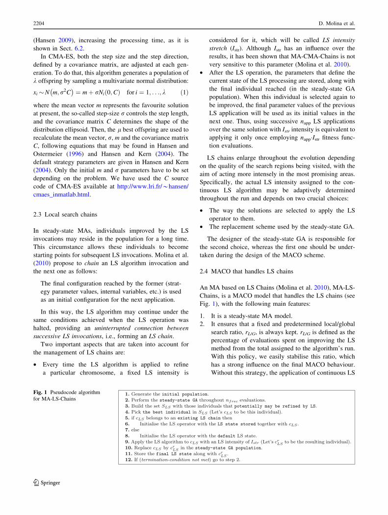
2.4 MACO that handles LS chains

An MA based on LS Chains (Molina et al. 2010), MA-LS-

Chains, is a MACO model that handles the LS chains (see

Fig. 1), with the following main features:

1. It is a steady-state MA model.

2. It ensures that a fixed and predetermined local/global

search ratio, rL/G, is always kept. rL/G is defined as the

percentage of evaluations spent on improving the LS

method from the total assigned to the algorithm’s run.

With this policy, we easily stabilise this ratio, which

has a strong influence on the final MACO behaviour.

Without this strategy, the application of continuous LS

Fig. 1 Pseudocode algorithm

for MA-LS-Chains


123

http://www.lri.fr/~hansen/cmaes_inmatlab.html

http://www.lri.fr/~hansen/cmaes_inmatlab.html

algorithms may induce the MACO to prefer super

exploitation.

3. It favours the enlargement of those LS chains that are

showing promising fitness improvements in the best

current search areas represented in the steady-state GA

population. In addition, it encourages the activation of

innovative LS chains with the aim of refining unex-

ploited zones, whenever the current best ones may not

offer profitability. The criterion to choose the individ-

uals that should undergo LS is specifically designed to

manage the LS chains in this way (Steps 3 and 4).

MA-LS-Chains defines the following relation between

the steady-state GA and the LS method (Step 2): every nfrec

number of evaluations of the steady-state GA, apply the

continuous LS algorithm to a selected chromosome, cLS, in

the steady-state GA population. Since we assume a fixed

local/global ratio, rL/G, nfrec must be automatically calcu-

lated, as follows:

nfrec ¼ Istr

1� rL=G

rL=G

ð2Þ

where Istr is the LS intensity stretch (Sect. 2.3). Step 3 and

4 require a greater explanation:

– SLS described in Step 3 is the set of individuals in the

steady-state GA population that fulfils:

(a) They have never been optimised by the LS

algorithm, or

(b) They previously underwent LS, obtaining a fitness

function improvement greater than dLSmin (a param-

eter of the algorithm).

– If |SLS| = 0, in Step 4, we select cLS as the individual

in this set with best fitness. In other case, the population

of the steady-state MA is randomly restarted consider-

ing all the search domain (except the best individual,

which is kept in the population to preserve the elitist

criterion).

With this mechanism, when the steady-state GA finds a

new best individual, it will be refined immediately. Fur-

thermore, the best performing individual in the steady-state

GA population will always undergo LS whenever the fit-

ness improvement obtained by a previous LS application to

this individual is greater than a dLSmin threshold.

2.5 MA-CMA-Chains: MA-LS-Chains with CMA-ES

MA-CMA-Chains (Molina et al. 2010) is an MA-LS-

Chains using the CMA-ES algorithm as the LS method. In

MA-CMA-Chains, the CMA-ES parameters in Eq. 1 are

automatically set as following:

– We consider the current solution to improve (cLS) as

the initial mean of distribution (m!).

– The initial r value is half the distance of cLS to its

nearest individual in the steady-state GA population

(this value allows an effective exploration around cLS).

CMA-ES will work as a local searcher consuming Istr

fitness function evaluations. Then, the resulting solution

will be introduced in the steady-state GA population along

with the current covariance matrix, the mean of the dis-

tribution, the step-size, and the variables used to guide the

adaptation of these parameters (B, BD, D, pc, and pr)

(Hansen 2010). Later, when CMA-ES is applied to this

inserted solution, these values will be recovered to proceed

with a new CMA-ES application. When CMA-ES is

applied to solutions that do not belong to existing chains,

default values, given by Hansen and Kern (2004), are

assumed for the remaining strategy parameters.

3 Continuous LS methods

In this section, we present a detailed description of dif-

ferent continuous LS methods used in our empirical study.

We have considered different types of algorithms:

– Several well-known continuous LS methods: Solis and

Wets’ algorithm (Solis and Wets 1981) and Nelder and

Mead’s simplex method (Nelder and Mead 1965). They

are interesting because they are LS methods that

explore randomly the neighbourhood of solutions,

considering all variables at the same time. Also, they

are classic LS methods used in the literate to build

different MACOs (Caponio et al. 2007; Gol-Alikhani

et al. 2009; Hongfeng and Guanzheng 2009).

– Specific continuous local searchers for large scale

problems, MTS-LS1 and MTS-LS2. They were pro-

posed for a particular algorithm, Multiple Trajectory

Search for Large Scale Global Optimisation (MTS)

proposed by Tseng and Chen (2008). These two LS

methods make the local exploration changing only one

variable, or a random subset of variables in each step of

the search, increasing or decreasing their values a

certain amount.

– The proposed SSW method, which combines the two

previous schemes. It uses a randomly exploration of the

local neighbourhood, like Solis and Wets’ algorithm,

but in each step of the algorithm only a subset of

variables is modified.

In the following subsections, we present a detailed

description of each one of these LS methods, paying spe-

cial attention to the characteristics that could be interesting

from the perspective of scalability.


123

3.1 Solis and Wets’ algorithm

The classic Solis and Wets’ algorithm (SW) (Solis and

Wets 1981) is a randomised hill-climber with an adaptive

step size. Each step starts at a current point x!: A deviate

d!

is chosen from a normal distribution whose standard

deviation is given by a parameter q. If either x!þ d!

or

x!� d!

is better, a move is made to the better point and

a success is recorded. Otherwise, a failure is recorded.

After several successes in a row, q is increased to move

more quickly. After several failures in a row, q is

decreased to focus the search. It is worth noting that q is

the strategy parameter of this continuous LS operator.

Additionally, a bias��!

term is included to put the search

momentum in directions that yield success. This is a

simple LS method that can adapt its step size very

quickly. The complete scheme is presented in Fig. 2,

where Sol is the solution to be refined and N is the

dimension. A more detailed explanation can be found in

Solis and Wets (1981).

3.2 Nelder and Mead’s Simplex algorithm

This is a classic and very powerful local descent algorithm.

A simplex is a geometrical figure consisting in n dimen-

sions, of n ? 1 points s0,…, sn. A point of a simplex is

taken as the origin, the other n points are used to describe

vector directions that span the n-dimension vector space.

Thus, if we randomly draw an initial starting point s0, then

we generate the other n points si according to the relation

si = s0 ? kej, where the ej are n unit vectors, and k is a

constant that is typically equal to one.

Through a sequence of elementary geometric transfor-

mations (reflection, contraction, expansion, and multi-con-

traction), the initial simplex moves, expands or contracts.

To select the appropriate transformation, the method only

uses the values of the function to be optimised at the ver-

tices of the simplex considered. After each transformation, a

better vertex replaces the current worst one. A complete

picture of this algorithm may be found in Nelder and Mead

(1965).

At the beginning of the algorithm, the point of the

simplex with the worst objective function is replaced, and

another point, the image of the worst one, is generated.

This is the reflection operation. If the reflected point is

better than all other points, the method expands the simplex

in this direction, otherwise, if it is at least better than the

worst one, the algorithm performs the reflection again with

the new worst point. The contraction step is performed at

the worst point, in such a way that the simplex adapts itself

to the function landscape and finally surrounds the opti-

mum. If the worst point is better than the contracted point,

the multi-contraction is performed. At each step we check

that the generated point is not outside the allowed reduced

solution space.

This method has the advantage of initially creating a

simplex composed of movements in each direction. This is

a useful characteristic to deal with high-dimensional

spaces, because this method can easily explore in all

directions, however, it requires a higher cost when the

dimension increases.

3.3 MTS-LS algorithms

Several classic LS methods may not scale well, thus they

are not able to obtain good results in large scale

Fig. 2 Pseudocode for Solis Wets’ algorithm


123

optimisation problems (Schwefel 1981). One option to

solve this problem is using an LS method specifically

designed for this type of problems.

In the CEC’2008 competition (Tang 2008) different

authors applied LS methods specially designed for this type

of problems. One of them is the Multiple Trajectory Search

algorithm (MTS) (Tseng and Chen 2008). MTS was

designed for multi-objective problems (Tseng and Chen

2007), but it has also proved to be a very good algorithm

for large scale optimisation problems, obtaining the best

results in the CEC’2008 competition (Tang 2008).

MTS applies a certain number of iterations of LS over a

population randomly initialised to create a simulated

orthogonal array. It applies to each individual I three LS

procedures, LS1, LS2, and LS3, obtaining three new solu-

tions, Ic1, Ic2, and Ic3. We call these LS procedures MTS-

LS1, MTS-LS2 and MTS-LS3, respectily, in order to avoid

any confusion with the previously described LS methods.

The original individual I is then replaced by the best of

these three new solutions. We have considered only the

first two LS methods, because MTS-LS3 is similar in

structure to the Solis Wets’ algorithm.

Both MTS-LS1 and MTS-LS2 are hill-climbing algo-

rithms that do not explore all dimensions at the same time.

In each step of MTS-LS1, each variable of the individual

to be refined is changed at a time. Each variable is

decreased by a certain value (called SR by Tseng and Chen

2008) to check if the objective function value is improved.

If the new solution improves the original one, the search

proceeds to consider the next dimension. If it is worse, the

original solution is restored and then the same variable is

increased by 0.5�SR to check if the objective function value

is improved again. If there is an improvement, the search

proceeds to consider the next dimension. In the other case,

the solution is restored and the search proceeds to consider

the next dimension.

MTS-LS2 has a structure very similar to MTS-LS1, with

two important differences. The first and crucial difference

is that MTS-LS1 explores all the solution components,

while MTS-LS2 explores changing at the same time a

quarter of solution components (randomly selected by

each application of the LS method). Another difference is

that the direction of exploration of each variable is ran-

domly selected for MTS-LS2. Figures 3 and 4 show in

detail the MTS-LS1 and MTS-LS2 methods, where Xk is

the solution to be improved, N is the dimension, and

[LOWER_BOUND, UPPER_BOUND] is the search

domain.

Although it could be expected that the LS methods that

explore dimension by dimension or only a subset of them

are only adequate to separable problems, in combination

with an EA that explores all variables at the same time, this

problem is reduced, as it is observed in Sect. 6.

3.4 Subgrouping Solis Wets’ algorithm

The previous LS methods can be divided into two groups.

– From the point of view of the modification of

variables. To create new solutions, Solis Wets’ and

Simplex algorithms modify current solutions by a

difference vector randomly generated (and in the case

Fig. 3 Pseudocode for MTS-LS1


123

of Solis Wets’ algorithm maintaining a direction

vector bias��!

). MTS-LS1 and MTS-LS2 modify the

current solution increasing or decreasing a certain

fixed value that is changed when the solution is not

improved. This characteristic could make algorithms

in the first group more adaptable to functions in which

the contribution of the variables over the fitness value

can differ.

– From the point of view of the number of variables

improved in each step of the search. Solis Wets’ and

Simplex algorithms explore all variables at the same

time, when MTS-LS1 modified only one variable, and

MTS-LS2 changes a subset of variables.

In this way, MTS-LS1 and MTS-LS2 change quicker

the values of the variables that improve the fitness. This

characteristic makes them more appropriated for sep-

arable functions, and, at the same time, they could

accelerate the speed of convergence in several non-

many-separable large scale problems (problems with

several separable variables). On the other hand, Solis

Wets’ and Simplex algorithms can better improve the

non-separable functions.

In this section, we propose a new LS method to combine

these characteristics:

– Creation of a new individual using a vector of

differences randomly generated around a small area.

This model could be more useful when it is used in

combination with a memetic algorithm. To do this, we

use the global scheme of Solis Wets’ algorithm.

– Not exploring all variables at the same time, but a

random subset of consecutive variables at each time. In

this way, the algorithm can reduce the problems,

achieving better results. For each number of evalua-

tions, the subset of variables to be improved is changed.

Although in general this could be a limitation, it is not

actually the case with the model proposed in Sect. 2,

because the same individual could be improved several

times by the LS method, using several groups of

variables at each time.

The objective of this LS method is to be more robust

than previous LS methods when is used with the MACO

model presented in Sect. 2, to avoid obtaining very good

results in a group of functions at the cost of getting worse

in the other group.

The detailed algorithm, that we call Subgrouping Solis

Wets’ algorithm is shown in Fig. 5, where Sol is the

solution to be refined and N is the dimension. It uses a

similar algorithm than Fig. 2 but in each step only the

random difference of a subset of variables (identified by a

vector change) is generated. This subset is randomly

updated every maxEvalSubSet evaluations. For the otherFig. 4 Pseudocode for MTS-LS2


123

variables, there is no difference vector. They are only

modified by the bias parameter, thus they naturally move

during certain evaluations (defined by the decreasing

mechanism of variable bias��!

).

The number of variables to be changed is set to 20% of

the number of solution components, considering a maxi-

mum number of maxVars = 50 variables.

This subset of variables to explore is maintained during

a certain number of evaluations, maxEvalSubSet. This

parameter sets the number of evaluations invested in each

random subset.

4 Proposed MAs based on LS chains for large scale

continuous optimisation problems

In this section, we present a detailed description of the

different proposed MAs based on LS Chains used in our

study. They use the same structure defined in Sect. 2, but

instead of using the CMA-ES algorithm described in

Sect. 2.2, they apply a different LS method. Each one of

the proposed MAs based on LS Chains differ only in the

LS method applied. Thus, comparing these different pro-

posals we are comparing the advantages of using each one

of the considered LS methods.

The different proposed MAs based on LS Chains are

named MA-LS-Chains, where LS is the LS method applied.

We have considered five instances:

– MA-SW-Chains, that applies the Solis and Wets’

algorithm (Sect. 3.1).

– MA-Simplex-Chains, that applies the Nelder and

Mead’s simplex method (Sect. 3.2).

– MA-MTSLS1-Chains, that applies the MTS-LS1 algo-

rithm (Sect. 3.3).

– MA-MTSLS2-Chains, that applies the MTS-LS2 algo-

rithm (Sect. 3.3).

– MA-SSW-Chains, that applies the Subgrouping Solis

Wets’ algorithm (Sect. 3.4).

– MA-CMA-Chains, that applies the CMA-ES algorithm

(Sect. 2.2).

In the following, we describe the common features of

the different considered MA-LS-Chains, and then we

describe each one of them, indicating their specific

parameters (MA-CMA-Chains was completely described

in Sect. 2).

4.1 Common features

In this section, we list the common features of the different

MAs based on LS Chains:Fig. 5 Pseudocode for subgrouping Solis Wets’ algorithm


123

4.1.1 Steady-state GA

It is a real-coded steady-state GA (Herrera et al. 1998)

specifically designed to promote high population diversity

levels by means of the combination of the BLX-a crossover

operator (see Herrera et al. 1998) with a high value for its

associated parameter (a = 0.5) and the negative assorta-

tive mating strategy (Fernandes and Rosa 2001). Diversity

is also favored by means of the BGA mutation operator

(see Herrera et al. 1998).

4.1.2 Continuous LS algorithms

The MA instances follow the MACO approach that handles

LS chains, with the objective of tuning the intensity of the

LS algorithms considered, which are employed as contin-

uous LS operators.

4.1.3 Parameter setting

For the experiments, the population size is 100 individuals

and the probability of updating a chromosome by mutation

is 0.125. The nass parameter associated with the negative

assortative mating is set to 3. They use Istr = 500. Finally,

a value of dLSmin= 0 (threshold value) has been applied.

These parameter values are recommended by Molina et al.

(2010).

4.2 MA-SW-Chains

MA-SW-Chains is an MA based on LS chains that uses as

its improvement method the Solis and Wets’ algorithm

described in Sec. 3.1. The parameters that guide the search

are the following (they will be stored with the individuals):

– The current direction value, called bias��!

in the descrip-

tion. Its default value is the vector 0!; thus it does not

initially have a direction by default, it will obtain it

during the search.

– The variance q, which sets the step size. The initial

value of this parameter can have a real influence over

the results. The default value for a new individual is

half of the distance to its nearest neighbour.

4.3 MA-Simplex-Chains

MA-Simplex-Chains is an MA based on LS chains that

uses as its improvement method the Simplex algorithm

described in Sect. 3.2. The parameters that guide the search

are:

– The simplex structure. Initially the solutions of this

structure are created by increasing in one dimension the

initial solution by a certain value, creating a simplex

with n elements, as described in Sect. 3.2. In our

experiment k = 10% of the domain.

– The fitness from each solution contained in the simplex

structure.

4.4 MA-MTSLS1-Chains and MA-MTSLS2-Chains

MA-MTSLS1-Chains and MA-MTSLS2-Chains are MAs

based on LS chains that use MTS-LS1 and MTS-LS2

(Sect. 3.3) as improvement methods. The main parameter

that guides the search is the initial d value, which will be

stored with the individuals. The default value for a new

individual is half of the distance to its nearest neighbour.

This parameter has a minimum and a maximum value, set

to 0.4 and 1e-15, respectively, suggested by Tseng and

Chen (2008).

4.5 MA-SSW-Chains

MA-SSW-Chains is an MA based on LS chains that uses as

improvement method the Subgrouping Solis and Wets’

algorithm described in Sect. 3.4. The parameters that guide

the search are the following:

– The current direction value, called bias��!

in the descrip-

tion. Its default value is the vector 0!

, thus it does not

initially have a direction by default, it will be adapted

during the search.

– The variance q, which sets the step size. The initial

value of this parameter can have a real influence over

the results. The default value for a new individual is

half of the distance to its nearest neighbour.

– The number of variables to change in each step is set to

20% of the solution components, considering a max-

imum number of maxVars = 50 variables.

– maxEvalSubSet is initialised as maxEval/10, to allow

the LS method to explore 10 different subsets of

variables at each step.

5 Experimental setup and statistical analysis

In this section, we present the experimental study carried

out on the MACO algorithms described in Sect. 4. The test

suite used is proposed by the organizers of the special

issue Scalability of Evolutionary Algorithms and other

Metaheuristics for Large Scale Continuous Optimization

Problems in the journal Soft Computing, whose description

and source code is available at http://sci2s.ugr.es/

eamhco/CFP.php. This has the great advantage that, fol-

lowing its conditions, the different proposals presented in


123

http://sci2s.ugr.es/eamhco/CFP.php


this special issue are comparable, allowing other authors to

follow the same test suite and compare their results with

those obtained by all previous algorithms using the same

test suite.

In the following, we are going to describe its main

characteristics. http://sci2s.ugr.es/eamhco/CFP.php can be

consulted for a more detailed description. The test suite

is composed of 19 scalable function optimization

problems:

1. Six functions: f1–f6, proposed for the Special Session

for Large Scale Problems on the IEEE Congress on

Evolutionary Computation (CEC’2008). A detailed

description may be found in Tang et al. (2007).

2. Five additional shifted functions: Schwefels Problem

2.22 (f7), Schwefels Problem 1.2 (f8), Extended f10 (f9),

Bohachevsky (f10), and Schaffer (f11).

3. Eight hybrid composition functions (f12–f19). They are

non-separable functions built by the combination of

one separable function of the previous ones with a non-

separable function of the previous ones. The influence

of the non-separable function is greater when the

function number increases.

Because the behaviour of the algorithms on separable

functions is a useful feature, in our analysis we are going to

study the behaviour of the algorithms considering all

functions, and in two groups:

– First 11 functions (f1–f11), to test the behaviour of the

algorithms on well-know functions.

– Hybrid compositions functions (f12–f19), to test the

behaviour of the algorithms in separable functions, with

increasing difficulty, in which the influence of the

variables over the final results is not the same.

All the experiments have been carried out following the

instructions indicated in the test suite specifications. The

experimental conditions in the test suite are the following:

1. Each function is tested with dimensions D = 50,

D = 100, D = 200, D = 500, and D = 1,000.

2. The stopping criterion is the maximum number of

fitness evaluations. This value is 5,000�D. Each run

stops when the maximum number of evaluations is

achieved, or when an error lower than 10-14 is

achieved.

3. Each algorithm is run 25 times for each test function,

and the error of the best individual of the population is

computed. The function error measure is defined as

(f(x) - f(x*) ), where x* is the global optimum of the

function.

4. The performance measures provided are:

– Average of error value found in the 25 runs.

– Maximum error achieved in the 25 runs.

– Minimum error achieved in the 25 runs.

– Median of the error achieved in the 25 runs.

To analyse the results we have used non-parametric

tests, because it has been shown that parametric tests

cannot be applied with security for several of the functions

used in the test suite (Garcıa et al. 2009a, b; Garcıa and

Herrera 2008). We have applied the non-parametric test

recommended by Garcıa et al. (2009b), thus this paper and

the website http://sci2s.ugr.es/sicidm/ can be consulted in

order to obtain a detailed explanations of them. Next, these

tests are briefly explained:

– The Iman-Davenport’s test. This non-parametric test is

used to answer this question: in a set of k samples

(where k C 2), do at least two of the samples represent

populations with different median values? It is a non-

parametric procedure employed in a hypothesis testing

situation involving a design with two or more samples;

therefore, it is a multiple comparison test that aims to

detect significant differences between the behaviour of

two or more algorithms.

– The Holm’s test as a post hoc procedure, to detect

which algorithms are worse than the algorithm with the

best results. This test can only be applied if the Iman-

Davenport’s test detects a significant difference. It

sequentially checks the hypotheses ordered according

to their significance. If pi is lower than a/(k - i), the

corresponding hypothesis is rejected and the process

continues. In the other case, this hypothesis and all the

remaining hypotheses are maintained as supported.

– The Wilcoxons test is used for answering this question:

do two samples represent two different populations? It is

a non-parametric procedure employed in a hypothesis

testing situation involving a design with two samples. It

is a pairwise test that aims to detect significant differ-

ences between the behaviour of two algorithms.

In the following, we describe the test computations. Let

di be the difference between the performance scores of

the two algorithms on ith out of N functions. The

differences are ranked according to their absolute

values; average ranks are assigned in case of ties. Let

R? be the sum of ranks for the functions in which the

second algorithm outperformed the first, and R- the

sum of ranks for the opposite. Let T be the smallest of

the sums, T = min(R? , R-). If T is less than or equal to

the value of the distribution of the Wilcoxon for


123


http://sci2s.ugr.es/sicidm/

N degrees of freedom (Table B.12 in Zar 1999), then the

null hypothesis of equality of means is rejected.

6 Analysis of results

In this section, we analyse the results obtained from different

experimental studies carried out with the MA-LS-Chains

instances. In particular, our aims are: (1) to calculate the best

ratio rL/G (Sect. 6.1), (2) to investigate the CPU processing

time and the scalability of each algorithm (Sect. 6.2), and (3)

to identify which MA-LS-Chains (and LS method) obtains

the best results (Sect. 6.3).

6.1 Selection of parameter rL/G

Molina et al. (2010) considered that the best value for rL/G

is 0.5. However, that parameter tuning was made with the

CMA-ES algorithm as LS operator, and without consider-

ing a high dimension value and its influence over the LS

method.

In this section, we compare the results of each MA-LS-

Chains using different values for rL/G: 0.2, 0.5, and 0.8.

Figures 6, 7, 8, 9, 10 and 11 show the average ranking

obtained by each MA-LS-Chains instance and dimension.

Each column represents the average ranking by an algo-

rithm; that is, if a certain algorithm achieves rankings 1, 3,

1, 4, and 2, on five test functions, the average ranking is1þ3þ1þ4þ2

5¼ 11

5: The height of each column is proportional

to the ranking. Therefore, the lower a column is, the better

Fig. 6 Average ranking for MA-CMA-Chains for each dimension

Fig. 7 Average ranking for MA-MTSLS1-Chains for each dimension

Fig. 8 Average ranking for MA-MTSLS2-Chains for each dimension

Fig. 9 Average ranking for MA-Simplex-Chains for each dimension

Fig. 10 Average ranking for MA-SW-Chains for each dimension

Fig. 11 Average ranking for MA-SSW-Chains for each dimension


123

its associated algorithm is. From these figures we can see

that rL/G = 0.8 is the best choice for every instance. This

was expected, because with a higher search domain, a

higher LS exploitation could improve the results. Also, it

can be observed that:

– For MA-CMA-Chains, for dimension 50 the best value

is rL/G = 0.5 and for dimension 100 the differences

with rL/G = 0.8 are very reduced, which is consistent

with the results obtained in Molina et al. (2010). For

higher dimensionality, rL/G = 0.8 is consolidated as the

best value.

– rL/G parameter has a great influence on the results. In all

cases, the best results are obtained with greater rL/G.

– For MA-MTSLS1-Chains, the rL/G influence strongly

depends on the dimensionality. For lower values, the

rL/G influence is very small, and for 500 and 1,000

dimensions there are significant differences in function

of rL/G parameter.

– For MA-MTSLS2-Chains, the rL/G influence is very

similar for each dimension. The fact that they do not

consider all components at the same time could be the

reason for that behaviour.

– For MA-SSW-Chains, the rL/G influence is reduced

when the dimension is under 200, for higher dimension

values the differences increase with the dimensionality.

In conclusion, we can observe that for all the algorithms

the best value for rL/G is 0.8, particularly when the

dimensionality is increased. Thus, in the following sec-

tions, we will use rL/G = 0.8.

6.2 Measuring the processing time

A crucial requirement of an LS method for large scale

optimisation is to have good scalability. In this section, we

have compared the processing time of each MACO for

each dimensionality.

In the experimental specifications the main stopping

criterion is the maximum number of evaluations. Consid-

ering this criterion, the differences in time between the

different algorithms could not be considered. However, in

real large scale problems, this requirement is crucial to

consider an algorithm to be a scalable one. Thus, we are

going to measure the processing time by each algorithm to

test its scalability, observing how much the cost time

increases when dimensionality is increased.

Table 1 shows these results, using only the maximum

number of evaluations as criterion (not considering the

threshold value). All the experiments have been made in C/

C?? using gcc 4.1.2, and they have been run with an Intel

Xeon CPU with 3 GHz, under GNU/Linux kernel

2.6.16.54 for SMP machines.

Table 1 measures the total time, Ttotal, and this value

could be due to different components. In Table 2, we show

the mean processing time spent by the LS methods, TLS,

and the value 100�TLS/Ttotal.

From Table 1 we can see that the high processing time

with MA-CMA-Chains makes it unable to tackle high

dimensional problems. The required times for the other

instances are very similar.

From Table 2, we can see that CMA-ES requires the

majority of the processing time of MA-CMA-Chains,

achieving more than 90% of total time when dimension-

ality is [500. Thus, the high CPU cost is due mainly to

CMA-ES. The main reason for that excessive time

requirement is the use of a high computing costs operation,

eigen-decomposition, which is a very expensive mathe-

matical operation with complexity D3 (Hansen 2009).

Thus, CMA-ES is not suitable for high dimensional

problems.

Table 1 Mean timing for each

instance and dimension

Bold values indicate the worst

time

LS method D = 50 D = 100 D = 200 D = 500 D = 1,000

MA-CMA-Chains 5.67 s 17.82 s 1 min 43 s 29 min 32 s 8 h 32 min

MA-MTSLS1-Chains 2.44 s 10.49 s 38.40 s 3 min 42 s 16 min 09 s

MA-MTSLS2-Chains 2.62 s 10.35 s 39.42 s 4 min 01 s 15 min 51 s

MA-Simplex-Chains 2.40 s 9.40 s 39.53 s 3 min 36 s 15 min 55 s

MA-SW-Chains 2.61 s 11.29 s 42.32 s 4 min 03 s 17 min 05 s

MA-SSW-Chains 2.64 s 9.58 s 33.71 s 3 min 21 s 14 min 07 s

Table 2 Mean 100�TLS/Ttotal, for each instance and dimension

LS method D = 50 D = 100 D = 200 D = 500 D = 1,000

CMA-ES 58.43 50.89 67.15 89.23 97.42

MTS-LS1 5.73 16.58 13.34 14.05 17.96

MTS-LS2 12.21 15.45 15.62 24.57 16.70

Simplex 4.16 6.91 16.00 11.66 17.30

Solis Wets 11.87 22.39 22.03 21.48 22.58

Subgrouping

Solis Wets

12.63 12.42 12.50 12.50 12.63


123

The second method that requires a higher processing

time is the Solis Wets’ method, that requires more than 20%

of the total time. The fastest LS method is Subgrouping

Solis Wets, followed by MTS-LS1 and MTS-LS2. Simplex

is initially very fast, but when dimension increases, it pre-

sents similar results to MTS-LS1 and MTS-LS2.

In conclusion, the CMA-ES method is not suitable for

high dimensional problems because of its high processing

time. That implies that MA-CMA-Chains proposed in the

previous work (Molina et al. 2010) is not able to tackle

large scale problems. Thus, it is confirmed that another LS

method needs to be selected that allows us to solve large

scale problems effectively.

Since the processing requirements for the remaining LS

methods are very similar, we analyse which ones give the

best results in the benchmark functions.

6.3 Comparison to obtain the best MA instance

In this section, we compare the different MA-LS-Chains in

the large-scale problems using the test suite previously

described.

First, we have applied the Iman-Davenport’s test to

check if there are significant differences between the

algorithms. Table 3 shows the results.

There is a statistically relevant difference for every

dimension, thus we apply the Holm’s test, considering the

algorithm with lowest average error as the control algo-

rithm. Table 4 shows the results, concluding that

MA-SSW-Chains is the best instance, and it is better than

all other algorithms: MA-MTSLS1-Chains, MA-MTSLS2-

Chains, MA-Simplex-Chains, and MA-SW-Chains. This

shows the convenience of the proposed SSW method.

We have obtained the average ranking comparing all

alternative MA instances to visualise the differences

between them. Fig. 12 shows the results considering all

functions, and Figs. 13 and 14 considering functions f1–f11

and f12–f19, respectively. We can observe that MA-SSW-

Chains is the instance that achieves the best results in all

functions, specially in classic functions. MA-SW-Chains is

the second best algorithms in classic functions, and

MA-Simplex-Chains achieves the best results in the hybrid

functions, when there are different degrees of separability.

In resume, MA-SSW-Chains is able to achieve the best

results or similar results to the best instance for each group.

This proves the convenience of the SSW method, by its

robustness for the different functions. Among the other

instances, there is no one better than the other ones in the

large-scale problems, and their performance depends on the

function category.

7 Comparison with other algorithms

In this section, we compare our proposal, MA-SSW-

Chains, with several algorithms presented by the organizers

of the special issue as reference algorithms. These algo-

rithms are DE with operators rand/1/exp (Storn and Price

1997), CHC (Eshelman et al. 1993), and IPOP-CMA-ES

(Auger and Hansen 2005b). In this comparison we are

going to use the results provided by the organizers in

http://sci2s.ugr.es/eamhco/CFP.php.

– Differential evolution (DE) (Storn and Price 1997). A

classic DE model was considered, with no parameter

adaptation, at all. The crossover operator applied was

rand/1/exp. The F and CR parameters were fixed to 0.5

and 0.9 values, respectively. An important decision for

the application of DE to large scale problems is the

Table 3 Results of the Iman-Davenport’s test for dimension 50, 100,

200, 500, and 1,000

Dimension Iman-Davenport

value

Critical

value

Significant

differences?

50 118.5126 2.49 Yes

100 79.5675 2.49 Yes

200 74.3011 2.49 Yes

500 92.1355 2.49 Yes

1,000 79.5675 2.49 Yes

Table 4 Comparison, using Holm’s test, of the MA instances versus

MA-SSW-Chains (control algorithm)

Dimension Local

search

z p value a/i Sig.

differences?

50 MTS-LS2 7.695 1.42E-14 0.0125 Yes

MTS-LS1 5.232 1.67E-7 0.0166 Yes

SW 3.283 1.03E-3 0.025 Yes

Simplex 2.770 5.60E-3 0.050 Yes

100 MTS-LS2 7.695 1.42E-14 0.0125 Yes

MTS-LS1 4.720 2.36E-6 0.0166 Yes

Simplex 3.283 1.03E-3 0.0250 Yes

SW 3.283 1.03E-3 0.0500 Yes

200 MTS-LS2 7.695 1.42E-14 0.0125 Yes

Simplex 4.309 1.64E-5 0.0166 Yes

MTS-LS1 4.001 6.30E-5 0.0250 Yes

SW 2.975 2.93E-3 0.0500 Yes

500 MTS-LS2 7.387 1.50E-13 0.0125 Yes

MTS-LS1 5.540 3.02E-8 0.0166 Yes

Simplex 3.386 7.10E-4 0.0250 Yes

SW 2.668 7.64E-3 0.0500 Yes

1,000 MTS-LS2 6.977 3.02E-12 0.0125 Yes

MTS-LS1 5.540 3.02E-8 0.0166 Yes

Simplex 2.873 4.07E-3 0.0250 Yes

SW 2.052 4.02E-2 0.0500 Yes


123


choice of the population size (popsize). Usually, this

parameter is set in function of the problem dimension

(10�D or 3�D). When DE tackles functions with high

dimensionality (500–1,000), this criterion is not ade-

quate, and a maximum limit should be fixed. For the

experiments, a population of 60 individuals was used.

This algorithm is very interesting because it creates

new solutions modifying only a subset of variables.

– The algorithm CHC (Cross generational elitist selec-

tion, Heterogeneous recombination, and Cataclysmic

mutation) has also been defined for binary representa-

tion (Eshelman 1991) as for real-coding representation

(Eshelman et al. 1993). Real-coded CHC is based on

the same four main components of the classic CHC.

The elitist selection is exactly the same in both cases.

To identify if two solutions are too closed to be crossed

they are binary coded using the Gray representation,

and their Hamming distance is compared with a

threshold value. The crossover operator used, BLX-a(Eshelman and Schaffer 1993), is considered to

substitute the original crossover operator. The original

parameter values are used: initial threshold = L/4, with

L = 20�Dim, a = 0.5, and popsize = 50.

– Restart CMA evolution strategy with increasing pop-

ulation size (IPOP-CMA-ES) (Auger and Hansen

2005b). The values considered for the algorithm

parameters were the ones suggested by Auger and

Hansen (2005b). The initial solution is uniform

randomly chosen from the domain search and the

initial distribution size (r) is a third of the domain size.

This algorithm has obtained very good results in the

2005 IEEE Congress on Evolutionary Computation

(Hansen 2005), showing itself to be a very good

algorithm for continuous optimization problems.

The original papers and http://sci2s.ugr.es/eamhco/

descriptions.pdf can be consulted to obtain a more

detailed explanation of these algorithms.

First, we detect if there are significant differences

between the reference algorithms, DE, IPOP-CMAES, and

CHC, and the proposal, MA-SSW-Chains. Table 5 shows

the results of Iman-Davenport’s test comparing the

Fig. 12 Average ranking for

each MA-LS-Chains instance

and dimension, f1–f19








123

http://sci2s.ugr.es/eamhco/descriptions.pdf

http://sci2s.ugr.es/eamhco/descriptions.pdf

previous algorithms for each dimension. We compare only

until dimension 500, because there are no results from

IPOP-CMAES for dimension 1,000. We can observe that

there are significant differences in any dimension, thus we

are going to use the Holm’s test for each dimension.

In Table 6, we present the Holm’s test results (DE is the

control algorithm, because it has the best average ranking).

For all the dimension values, DE is statistically better than

IPOP-CMAES and CHC, however, this test did not find

significant differences between DE and our algorithm.

In Tables 7, 8, and 9, we compare MA-SSW-Chains with

the different reference algorithms, CHC, IPOP-CMAES,

and DE, respectively, by means of the Wilcoxon’s test,

which is more powerful to identify differences between two

algorithms. We can observe that: (1) MA-SSW-Chains is

statistically better than CHC for all the dimensions, (2) it

outperforms statistically IPOP-CMAES for dimensions 50

and 100, and (3) DE is statistically better than MA-SSW-

Chains for the highest dimensions (200, 500, and 1,000). We

have also compared our algorithm and DE considering the

median error values (Table 10). In this case, we can observe

that there are not significant differences among them for all

dimensions, with regards to this performance measure.

8 Conclusions

In this paper, we have built several instances of MACO

based on LS chains that differ in the continuous LS method

applied: the Solis and Wets’s algorithm, the Nelder and

Mead’s simplex method, the MTS-LS1 and MTS-LS2

methods, the CMA-ES algorithm, and a new LS method,

the Subgrouping Solis Wets’ method.

Table 5 Results of the Iman-Davenport’s test of MA-SSW-Chains

and the reference algorithms for dimensions 50, 100, 200, and 500

Dimension Iman-Davenport

value

Critical

value

Significant

differences?

50 5.232034 2.46 Yes

100 3.256133 2.46 Yes

200 2.707457 2.46 Yes

500 2.820250 2.46 Yes

Table 6 Comparison of DE (control algorithm) with CHC, IPOP-

CMAES, and MA-SSW-Chains (Holm’s test)

Dimension Algorithm z p value a/i Sig.

dif-

ferences?

50 CHC 4.461 8.17E-06 0.017 Yes

IPOP-CMAES 2.827 4.69E-03 0.025 Yes

MA-SSW-Chains 0.251 8.02E-01 0.050 No

100 CHC 4.837 1.31E-6 0.017 Yes

IPOP-CMAES 3.08 2.08E-3 0.025 Yes

MA-SSW-Chains 0.628 0.53 0.050 No

200 CHC 4.963 6.93E-7 0.017 Yes

IPOP-CMAES 3.079 2.08E-3 0.025 Yes

MA-SSW-Chains 1.005 0.31 0.050 No

500 CHC 5.780 7.46E-9 0.017 Yes

IPOP-CMAES 2.890 3.85E-3 0.025 Yes

MA-SSW-Chains 1.634 0.102 0.050 No

Table 7 MA-SSW-Chains versus CHC using the average error

(Wilcoxon’s test with p value = 0.05)

Dimension R? R- Critical value Sig. differences?

50 185 5 46 Yes

100 190 0 46 Yes

200 190 0 46 Yes

500 190 0 46 Yes

1000 172 18 46 Yes

Table 8 MA-SSW-Chains versus IPOP-CMAES using the average

error (Wilcoxon’s test with p value = 0.05)


50 148 42 46 Yes

100 148 42 46 Yes

200 139 51 46 No

500 134 56 46 No

Table 9 MA-SSW-Chains versus DE using the average error (Wil-

coxon’s test with p value = 0.05)


50 71.5 118.5 46 No

100 55.5 134.5 46 No

200 43.5 146.5 46 Yes

500 12.0 178.0 46 Yes

1,000 37.0 153.0 46 Yes

Table 10 DE versus MA-SSW-Chains using the median values

(Wilcoxon’s test with p value = 0.05)


50 109.5 80.5 46 No

100 95.5 94.5 46 No

200 83.5 106.5 46 No

500 50.0 140.0 46 No

1,000 54.0 136.0 46 No


123

We have compared their performance and results on a

specific test suite, including problems with different

dimensions. The main conclusions obtained comparing our

instances with each other are:

– For high-dimensional problems, the best results have

been obtained giving more evaluations to the LS method.

– CMA-ES is not able to tackle large scale problems, due

to its spending time.

– The dimensionality strongly affects the performance of

the MACO instances based on the different LS

methods; not only in results, but also in processing

time. For low and medium-dimension the CMA-ES

algorithm is better, and for high-dimension, for results

and time cost, the other LS methods are better.

– No one of the selected LS methods from the literature

(MTS-LS1, MTS-LS2, Simplex, and Solis Wets’

methods) was better than the other ones.

– We have presented a variant of Solis Wets’ method,

Subgrouping Solis Wets’ method. This algorithm

explores a random subset of variables during a certain

number of evaluations. In combination with the LS

Chaining, this LS method has allowed our algorithm to

obtain better results than the considered LS methods

from the literature.

Then, we have compared our algorithm with algorithms

selected from the literature, concluding that the results

obtained by our algorithm are very competitive. Only DE

obtains better results than our algorithm, and there is no

statistically difference for the majority of the dimensions.

In conclusion, we have presented a new MACO based

on LS chains, MA-SSW-Chains, that is scalable for high-

dimensional problems and that obtains better results for

that type of problem than the original MACO based on LS

chains (Molina et al. 2010). The proposal is a very com-

petitive optimisation algorithm for large scale problems,

both in results and in processing time. In future work, we

will explore another EA components, such as differential

evolution, which could provide better results for large scale

problems than GAs.

Acknowledgments This work was supported by Research Projects

TIN2008-05854 and P08-TIC-4173.

Appendix

Tables 11, 12, 13, 14, 15, 16 show the average errors

obtained by MA-SSW-Chains, MA-MTSLS1-Chains, MA-

MTSLS2-Chains, MA-Simplex-Chains, MA-SW-Chains,

and MA-CMA-Chains, respectively.

Table 11 Average error obtained by MA-SSW-Chains for each

dimension

Function D = 50 D = 100 D = 200 D = 500 D = 1000

f1 0.00E?00 0.00E?00 0.00E?00 0.00E?00 0.00E?00

f2 2.57E-01 5.28E?00 4.15E?01 8.15E?01 1.39E?02

f3 3.63E?01 1.87E?02 1.82E?02 6.20E?02 1.12E?03

f4 0.00E?00 5.10E-13 8.95E?00 1.63E?02 1.63E?03

f5 0.00E?00 0.00E?00 0.00E?00 0.00E?00 0.00E?00

f6 0.00E?00 0.00E?00 1.14E-13 2.56E-13 1.85E-09

f7 0.00E?00 0.00E?00 0.00E?00 4.57E-14 6.51E-13

f8 1.33E-01 8.89E?01 7.86E?02 1.40E?04 7.38E?04

f9 2.91E?02 5.62E?02 1.17E?03 3.00E?03 6.03E?03

f10 0.00E?00 0.00E?00 0.00E?00 0.00E?00 0.00E?00

f11 1.70E-07 1.34E-01 4.12E-01 3.65E?00 4.40E?01

f12 0.00E?00 0.00E?00 3.03E-02 4.10E-02 1.21E-01

f13 3.73E?01 8.43E?01 1.83E?02 6.28E?02 9.35E?02

f14 0.00E?00 0.00E?00 1.65E-14 5.58E?01 7.49E?02

f15 0.00E?00 0.00E?00 0.00E?00 3.48E-14 1.15E-13

f16 0.00E?00 4.10E-02 6.06E-02 9.09E-02 7.38E-01

f17 3.83E?00 1.94E?02 2.43E?01 2.54E?02 3.02E?02

f18 0.00E?00 0.00E?00 0.00E?00 1.07E-02 4.84E?00

f19 0.00E?00 0.00E?00 0.00E?00 0.00E?00 4.47E-13

Table 12 Average error obtained by MA-MTSLS1-Chains for each

dimension

Function D = 50 D = 100 D = 200 D = 500 D = 1000

f1 0.00E?00 0.00E?00 0.00E?00 0.00E?00 1.69E-06

f2 1.71E-03 6.77E?00 2.54E?01 1.08E?02 1.36E?02

f3 9.28E?01 1.39E?02 3.22E?02 6.32E?02 3.61E?03

f4 0.00E?00 0.00E?00 4.06E-08 2.99E?02 8.70E?02

f5 0.00E?00 0.00E?00 0.00E?00 0.00E?00 3.85E-09

f6 5.68E-14 8.53E-14 1.71E-13 5.12E-13 5.04E-05

f7 0.00E?00 0.00E?00 0.00E?00 3.78E-14 1.01E-09

f8 9.18E?01 7.75E?01 2.04E?03 5.41E?05 3.59E?06

f9 2.89E?02 5.65E?02 1.18E?03 2.94E?03 5.79E?03

f10 0.00E?00 0.00E?00 0.00E?00 0.00E?00 1.03E-06

f11 0.00E?00 1.12E-01 4.64E-01 7.66E-01 6.91E?01

f12 0.00E?00 0.00E?00 0.00E?00 0.00E?00 1.51E?01

f13 3.26E?01 6.49E?01 2.21E?02 4.48E?02 9.95E?02

f14 0.00E?00 1.13E-10 8.54E-06 1.12E?01 3.78E?02

f15 0.00E?00 0.00E?00 0.00E?00 2.72E-14 1.56E-12

f16 0.00E?00 0.00E?00 0.00E?00 3.03E-02 2.85E-01

f17 6.81E-01 1.61E?01 3.58E?01 1.53E?02 3.50E?02

f18 0.00E?00 0.00E?00 0.00E?00 1.01E?00 3.91E?00

f19 0.00E?00 0.00E?00 0.00E?00 0.00E?00 2.65E-10


123

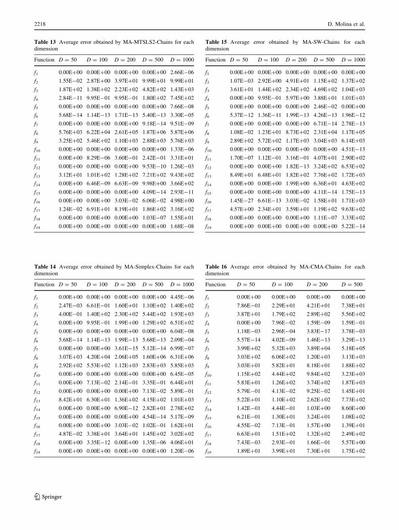
Table 13 Average error obtained by MA-MTSLS2-Chains for each

dimension

Function D = 50 D = 100 D = 200 D = 500 D = 1000

f1 0.00E?00 0.00E?00 0.00E?00 0.00E?00 2.66E-06

f2 1.55E-02 2.87E?00 3.97E?01 9.99E?01 9.99E?01

f3 1.87E?02 1.38E?02 2.23E?02 4.82E?02 1.43E?03

f4 2.84E-11 9.95E-01 9.95E-01 1.80E?02 7.45E?02

f5 0.00E?00 0.00E?00 0.00E?00 0.00E?00 7.66E-08

f6 5.68E-14 1.14E-13 1.71E-13 5.40E-13 3.30E-05

f7 0.00E?00 0.00E?00 0.00E?00 9.18E-14 9.51E-09

f8 5.76E?03 6.22E?04 2.61E?05 1.87E?06 5.87E?06

f9 3.25E?02 5.46E?02 1.10E?03 2.88E?03 5.76E?03

f10 0.00E?00 0.00E?00 0.00E?00 0.00E?00 1.33E-06

f11 0.00E?00 8.29E-06 3.60E-01 2.42E-01 3.31E?01

f12 0.00E?00 0.00E?00 0.00E?00 9.53E-10 1.26E-03

f13 3.12E?01 1.01E?02 1.28E?02 7.21E?02 9.43E?02

f14 0.00E?00 6.46E-09 6.63E-09 9.98E?00 3.66E?02

f15 0.00E?00 0.00E?00 0.00E?00 4.09E-14 2.93E-11

f16 0.00E?00 0.00E?00 3.03E-02 6.06E-02 4.98E?00

f17 1.24E-02 6.91E?01 8.19E?01 1.86E?02 3.16E?02

f18 0.00E?00 0.00E?00 0.00E?00 1.03E-07 1.55E?01

f19 0.00E?00 0.00E?00 0.00E?00 0.00E?00 1.68E-08

Table 14 Average error obtained by MA-Simplex-Chains for each

dimension

Function D = 50 D = 100 D = 200 D = 500 D = 1000

f1 0.00E?00 0.00E?00 0.00E?00 0.00E?00 4.45E-06

f2 2.47E-03 6.61E-01 1.60E?01 1.10E?02 1.40E?02

f3 4.00E-01 1.40E?02 2.30E?02 5.44E?02 1.93E?03

f4 0.00E?00 9.95E-01 1.99E?00 1.29E?02 6.51E?02

f5 0.00E?00 0.00E?00 0.00E?00 0.00E?00 6.04E-08

f6 5.68E-14 1.14E-13 1.99E-13 5.68E-13 2.09E-04

f7 0.00E?00 0.00E?00 3.61E-15 5.12E-14 6.99E-07

f8 3.07E?03 4.20E?04 2.06E?05 1.60E?06 6.31E?06

f9 2.92E?02 5.53E?02 1.12E?03 2.83E?03 5.85E?03

f10 0.00E?00 0.00E?00 0.00E?00 0.00E?00 6.45E-05

f11 0.00E?00 7.13E-02 2.14E-01 3.35E-01 6.44E?01

f12 0.00E?00 0.00E?00 0.00E?00 7.13E-02 5.89E-01

f13 8.42E?01 6.30E?01 1.36E?02 4.15E?02 1.01E?03

f14 0.00E?00 0.00E?00 6.90E-12 2.82E?01 2.78E?02

f15 0.00E?00 0.00E?00 0.00E?00 4.54E-14 5.17E-09

f16 0.00E?00 0.00E?00 3.03E-02 1.02E-01 1.62E?01

f17 4.87E-02 3.38E?01 3.64E?01 1.45E?02 3.02E?02

f18 0.00E?00 3.35E-12 0.00E?00 1.35E-06 4.06E?01

f19 0.00E?00 0.00E?00 0.00E?00 0.00E?00 1.20E-06

Table 15 Average error obtained by MA-SW-Chains for each

dimension

Function D = 50 D = 100 D = 200 D = 500 D = 1000

f1 0.00E?00 0.00E?00 0.00E?00 0.00E?00 0.00E?00

f2 1.07E-03 2.92E?00 4.91E?01 1.15E?02 1.37E?02

f3 3.61E?01 1.44E?02 2.34E?02 4.69E?02 1.04E?03

f4 0.00E?00 9.95E-01 5.97E?00 3.88E?01 1.01E?03

f5 0.00E?00 0.00E?00 0.00E?00 2.46E-02 0.00E?00

f6 5.37E-12 1.36E-11 1.99E-13 4.26E-13 1.96E-12

f7 0.00E?00 0.00E?00 0.00E?00 6.71E-14 2.78E-13

f8 1.08E-02 1.23E?01 8.73E?02 2.31E?04 1.17E?05

f9 2.89E?02 5.72E?02 1.17E?03 3.04E?03 6.14E?03

f10 0.00E?00 0.00E?00 0.00E?00 0.00E?00 4.51E-13

f11 1.70E-07 1.12E-01 3.16E-01 4.07E?01 2.90E?02

f12 0.00E?00 0.00E?00 1.82E-13 3.24E?02 6.53E?02

f13 8.49E?01 6.48E?01 1.82E?02 7.76E?02 1.72E?03

f14 0.00E?00 0.00E?00 1.99E?00 6.36E?01 4.63E?02

f15 0.00E?00 0.00E?00 0.00E?00 4.11E-14 1.75E-13

f16 1.45E-27 6.61E-13 3.03E-02 1.58E?01 1.71E?03

f17 4.57E?00 2.34E?01 3.59E?01 1.19E?02 9.63E?02

f18 0.00E?00 0.00E?00 0.00E?00 1.11E-07 3.33E?02

f19 0.00E?00 0.00E?00 0.00E?00 0.00E?00 5.22E-14

Table 16 Average error obtained by MA-CMA-Chains for each

dimension

Function D = 50 D = 100 D = 200 D = 500

f1 0.00E?00 0.00E?00 0.00E?00 0.00E?00

f2 7.86E-01 2.29E?01 4.21E?01 7.38E?01

f3 3.87E?01 1.79E?02 2.89E?02 5.56E?02

f4 0.00E?00 7.96E-02 1.59E-09 1.59E-01

f5 1.18E-03 2.96E-04 3.83E-17 3.78E-03

f6 5.57E-14 4.02E-09 1.46E-13 3.29E-13

f7 3.99E?02 5.32E?03 3.89E?04 5.18E?05

f8 3.03E?02 6.06E?02 1.20E?03 3.13E?03

f9 3.03E?01 5.82E?01 8.18E?01 1.88E?02

f10 1.15E?02 4.44E?02 9.84E?02 3.23E?03

f11 5.83E?01 1.26E?02 3.74E?02 1.87E?03

f12 5.79E-01 4.13E-02 9.25E-02 1.45E?01

f13 5.22E?01 1.10E?02 2.62E?02 7.73E?02

f14 1.42E-01 4.44E-01 1.03E?00 8.60E?00

f15 6.21E-01 1.30E?01 3.24E?01 1.08E?02

f16 4.55E-02 7.13E-01 1.57E?00 1.39E?01

f17 6.63E?01 1.51E?02 1.32E?02 2.49E?02

f18 7.43E-03 2.93E-01 1.66E-01 5.57E?00

f19 1.89E?01 3.99E?01 7.30E?01 1.75E?02


123

References

Auger A, Hansen N (2005a) Performance evaluation of an advanced

local search evolutionary algorithm. In: 2005 IEEE congress on

evolutionary computation, pp 1777–1784

Auger A, Hansen N (2005b) A restart CMA evolution strategy with

increasing population size. In: 2005 IEEE congress on evolu-

tionary computation, pp 1769–1776

van den Bergh F, Engelbrencht AP (2004) A cooperative approach

to particle swarm optimization. IEEE Trans Evol Comput

3:225–239

Caponio A, Cascella GL, Neri F, Salvatore N, Sumner M (2007) A

fast adaptive memetic algorithm for off-line and on-line control

design of PMSM drivers. IEEE Trans Syst Man Cybern B

37(1):28–41 (Special Issue on Memetic Algorithms)

Davis L (1991) Handbook of genetic algorithms. Van Nostrand

Reinhold, New York

Eshelman L (1991) The CHC adaptive search algorithm. How to have

safe search when engaging in nontraditional genetic recombina-

tion. In: Foundations of genetic algorithms, pp 265–283

Eshelman L, Caruana A, Schaffer JD (1993) Real-coded genetic

algorithms and interval-schemata. In: Foundation of genetic

algorithms, vol 2, pp 187–202

Eshelman LJ, Schaffer JD (1993) Real-coded genetic algorithms in

genetic algorithms by preventing incest. Foundation of genetic

algorithms, vol 2, pp 187–202

Fernandes C, Rosa A (2001) A study of non-random matching and

varying population size in genetic algorithm using a royal road

function. In: Proceedings of the 2001 congress on evolutionary

computation, pp 60–66

Garcıa S, Herrera F (2008) An extension on statistical comparisons of

classifiers over multiple data sets for all pairwise comparisons.

J Mach Learn Res 9:2677–2694

Garcıa S, Fernandez A, Luengo J, Herrera F (2009a) A study of

statistical techniques and performance measures for genetics-

based machine learning: accuracy and interpretability. Soft

Comput 13(10):959–977

Garcıa S, Molina D, Lozano M, Herrera F (2009b) A study on the use

of non-parametric tests for analyzing the evolutionary algo-

rithms’ behaviour: a case study on the CEC’2005 special session

on real parameter optimization. J Heuristics 15:617–644

Gol-Alikhani M, Javadian N, Tavakkoli-Moghaddam R (2009) A

novel hybrid approach combining electromagnetism-like method

with Solis and Wets local search for continuous optimization

problems. J Glob Optim 44(2):227–234

Goldberg DE, Voessner S (1999) Optimizing global-local search

hybrids. In: Banzhaf W et al (ed) Proceedings of the genetic and

evolutionary computation conference (GECCO 1999). Morgan

Kaufmann, San Mateo, California, pp 220–28

Hansen N (2005) Compilation of results on the CEC benchmark

function set. In: 2005 IEEE congress on evolutionary computation

Hansen N (2009) Benchmarking a BI-population CMA-ES on the

BBOB-2009 function testbed. In: GECCO’09: proceedings of

the 11th annual conference companion on genetic and evolu-

tionary computation conference, pp 2389–2396

Hansen N (2010) The CMA evolutionary strategy: a tutorial technical

report. The French National Institute of Research in Computer

Science and Control INRIA. http://www.lri.fr/*hansen/

cmatutorial.pdf

Hansen N, Kern S (2004) Evaluating the CMA evolution strategy on

multimodal test functions. In: Yao X et al (ed) Proceedings of

the parallel problem solving for nature—PPSN VIII, LNCS

3242. Springer, Berlin, pp 282–291

Hansen N, Ostermeier A (1996) Adapting arbitrary normal mutation

distributions in evolution strategies: the covariance matrix

adaptation. In: Proceeding of the IEEE international conference

on evolutionary computation (ICEC’96), pp 312–317

Hansen N, Muller SD, Koumoutsakos P (2003) Reducing the time

complexity of the derandomized evolution strategy with covari-

ance matrix adaptation (CMA-ES). Evol Comput 1(11):1–18

Hart WE (1994) Adaptive global optimization with local search. PhD

thesis, University of California, San Diego, CA

Herrera F, Lozano M (2000) Two-loop real-coded genetic algorithms

with adaptive control of mutation step sizes. Appl Intell

13(3):187–204

Herrera F, Lozano M, Verdegay JL (1998) Tackling real-coded

genetic algorithms: operators and tools for the behavioral

analysis. Artif Intell Rev 12(4):265–319

Hongfeng X, Guanzheng T (2009) High-dimension simplex genetic

algorithm and its application to optimize hyper-high dimension

functions. WRI global congress on intelligent systems, vol 2,

pp 39–43

Kennedy J, Eberhart RC (1995) Particle swarm optimization. In: IEE

international conference on neural networks, pp 1942–1948

Kita H (2001) A comparison study of self-adaptation in evolutionary

strategies and real-coded genetic algorithms. Evol Comput J

9(2):223–241

Krasnogor N, Smith JE (2001) Emergence of profitable search

strategies based on a simple inheritance mechanism. In:

Proceedings of the 2001 international conference on genetic

and evolutionary computation. Morgan Kaufmann, San Mateo,

California, pp 432–439

Krasnogor N, Smith JE (2005) A tutorial for competent memetic

algorithms: model, taxonomy, and design issue. IEEE Trans

Evol Comput 9(5):474–488

Land Shannon MW (1998) Evolutionary algorithms with local search

for combinational optimization. PhD thesis, University of

California, San Diego, CA

Lozano M, Herrera F, Krasnogor N, Molina D (2004) Real-coded

memetic algorithms with crossover hill-climbing. Evol Comput

12(2):273–302

Merz P (2000) Memetic algorithms for combinational optimization

problems: Fitness landscapes and effective search strategies. PhD

thesis, Gesamthochschule Siegen, University of Siegen, Germany

Molina D, Lozano M, Herrera F (2009) Memetic algorithm with local

search chaining for large scale continuous optimization prob-

lems. In: Proceedings of the 2009 IEEE congress on evolutionary


Molina D, Lozano M, Garcıa-Martınez C, Herrera F (2010) Memetic

algorithms for continuous optimization based on local search

chains. Evol Comput 18(1):27–63

Moscato PA (1989) On evolution, search, optimization, genetic

algorithms and martial arts: toward memetic algorithms. Tech.

rep., Technical report Caltech concurrent computation program

report 826. Caltech, Pasadena, California

Moscato PA (1999) Memetic algorithms: a short introduction.

McGraw-Hill, London, pp 219–234

Nelder JA, Mead R (1965) A simplex method for functions

minimizations. Comput J 7(4):308–313

Nguyen QH, Ong YS, Lim MH (2009) A probabilistic memetic

framework. IEEE Trans Evol Comput 13(3):604–623

Noman N, Iba H (2008) Accelerating differential evolution using an

adaptive local search. IEEE Trans Evoly Comput 12(1):107–125

Soon OY, Keane AJ (2004) Meta-lamarckian learning in memetic

algorithms. IEEE Trans Evolu Comput 4(2):99–110

Price KV, Storn RM, Lampinen JA (2005) Differential evolution: a

practical approach to global optimization. Springer, Berlin

Renders JM, Flasse SP (1996) Hybrid methods using genetic

algorithms for global optimization. IEEE Trans Syst Man

Cybern 26(2):246–258


123

http://www.lri.fr/~hansen/cmatutorial.pdf

http://www.lri.fr/~hansen/cmatutorial.pdf

Schwefel HP (1981) Numerical optimization of computer models.

Wiley, New York

Solis FJ, Wets RJ (1981) Minimization by random search techniques.

Math Oper Res 6:19–30

Storn R, Price K (1997) Differential evolution—a simple and efficient

heuristic for global optimization over continuous spaces. J Glob

Optim 11:341–359

Suganthan PN, Hansen N, Liang JJ, Deb K, Chen YP, Auger A,

Tiwari S (2005) Problem definitions and evaluation criteria for

the CEC 2005 special session on real parameter optimization.

Tech. rep., Nanyang Technical University. http://www.ntu.edu.

sg/home/epnsugan/index_files/CEC-05/Tech-Report-May- 30-05

Syswerda G (1989) Uniform crossover in genetic algorithms. In:

Schaffer JD (ed) Proceedings of the third international confer-

ence on genetic algorithms. Morgan Kaufmann, San Mateo,

pp 2–9

Tang K (2008) Summary of results on CEC’08 competition on large

scale global optimization. Tech. rep., Nature Inspired Compu-

tation and Application Lab (NICAL). http://nical.ustc.edu.cn/

papers/CEC2008_SUMMARY.pdf

Tang K, Yao X, Suganthan PN, MacNish C, Chen YP, Chen CM,

Yang Z (2007) Benchmark functions for the CEC’2008 special

session and competition on large scale global optimization.

Tech. rep., Nature Inspired Computation and Application

Laboratory, USTC, China. http://nical.ustc.edu.cn/cec08ss.php

Tseng LY, Chen C (2007) Multiple trajectory search for multiobjec-

tive optimization. In: 2007 IEEE congress on evolutionary


Tseng LY, Chen C (2008) Multiple trajectory search for large scale

global optimization. In: 2008 IEEE congress on evolutionary


Zar JH (1999) Biostatistical analysis. Prentice Hall, Englewood, NJ


123

http://www.ntu.edu.sg/home/epnsugan/index_files/CEC-05/Tech-Report-May- 30-05

http://www.ntu.edu.sg/home/epnsugan/index_files/CEC-05/Tech-Report-May- 30-05

http://nical.ustc.edu.cn/papers/CEC2008_SUMMARY.pdf

http://nical.ustc.edu.cn/papers/CEC2008_SUMMARY.pdf

http://nical.ustc.edu.cn/cec08ss.php

memetic algorithms based on local search chains for large scale … · 2015-04-07 · focus memetic...

Documents