mei statistics 2 - woodhouse...

MEI Statistics 2

© MEI, 16/02/11 1/7

The Poisson Distribution

Section 1: Introduction to the Poisson distribution Notes and Examples These notes contain subsections on

The Poisson distribution

Mean and variance of the Poisson distribution

The sum of two or more Poisson distributions

The Poisson distribution The Poisson distribution is useful in many situations and the standard conditions are that events occur

(i) randomly (ii) independently

and most importantly (always include in exam answers) (iii) at a uniform average rate of occurrence.

This is another example of a discrete probability distribution. You met the Binomial distribution in S1 and of course you met a whole chapter on discrete random variables also in S1. However, the key difference between the Poisson distribution and previous work is that it is an infinite probability distribution. There are many practical situations that can be modelled by a Poisson distribution:

The number of phone calls on a randomly chosen day

Insurance claims made by motorists in a given amount of time

Particles emitted by a radioactive source in a given amount of time

The number of cars passing in a randomly chosen 10 minute period on a road with no traffic problems (eg: no traffic lights)

The number of accidents in a factory per month

The number of typing errors on a randomly chosen page from a large document

You should be able to check that all these situations meet the conditions of events occurring randomly, independently and with a uniform average rate of occurrence. Sometimes these situations may not be appropriate: just because you can calculate a mean rate of something occurring does not mean the Poisson distribution is appropriate. Consider the following situations.

S2 Poisson section 1 Notes and Examples

© MEI, 16/02/11 2/7

Insurance claims in a town will not occur randomly after a period of flooding.

Cars passing in, say a 1 minute period, would not have a uniform mean rate of occurrence if controlled by sets of traffic lights.

The Poisson distribution has the following formula.

eP( )

!

r

X rr

This formula is given on page 9 of the formula book (MEI). λ is the mean (or expected value). You will meet e in your Core Maths units; it is the base of natural logarithms. Check on your calculator e1 = 2.71828… The upper case letter is a random variable; the lower case letter indicates a value it can take. This is an infinite distribution with r = 0, 1, 2, 3, …… You will need to use your previous probability work to work out examples such as P(X > 3). i.e. P(X > 3) = 1 - P(X 3) Example 1

The random variable X has a Poisson distribution with mean 2.

Find

(i) P(X = 1)

(ii) P(X = 4)

(iii) P(X 2)

Solution

In this case λ = 2.

(i) P( 1)X 2 1e 2

0.2711!

(ii) P( 4)X 2 4e 2

0.09024!

(iii) P( 2) 1 [P( 0) P( 1)]X X X

P( 0)X 2 0e 2

0.1350!

From (i) P( 1) 0.271X

P( 2)X 1 [0.135 0.271]

0.594


© MEI, 16/02/11 3/7

You can use the cumulative Poisson probability tables to work out a large number of probability calculations in one step. Example 2

The random variable X has a Poisson distribution with mean 1.80.

Find

(i) P(X 6 )

(ii) P(X > 4)

Solution

In this case λ = 1.80.

(i) P( 6) 0.9974X

(ii) P( 4)X 1 ( 4)

1 0.9636

0.0364

P X

Be careful how you use these tables, especially with the inequality signs. If the value of λ is not given in the tables, eg λ is 1.85 or λ is 12.0, you must calculate the probabilities, rather than take an approximate value from the tables.

The Autograph resource The Poisson distribution shows a graphical representation of the Poisson distribution and associated probabilities. For additional practice in finding Poisson probabilities, try the Poisson dominoes and the Poisson matching activity.

Mean and variance of a Poisson distribution You have already seen that the mean of a Poisson distribution with parameter λ is equal to λ. The Poisson distribution is unusual in that the parameter λ is also equal to the variance. So the Poisson distribution has equal values of the mean and variance. This property can help you decide if a Poisson distribution is a suitable model. Example 3

The following data were collected at the entrance to a Tourist Information office in a

French town Villeneuve. x is the number of visitors arriving per minute.

Look in the Poisson tables

under = 1.8 and x = 6

Look in the Poisson tables

under = 1.8 and x = 4


© MEI, 16/02/11 4/7

(i) Investigate whether the Poisson distribution is an appropriate model for these

data.

(ii) Calculate the expected frequencies for this distribution using a Poisson model.

Solution

(i) X is the distribution of the number of people visiting per minute.

Up to 3 people visited per minute, during the data collection of 43 minutes.

It would seem to be reasonable that X would be a Poisson distribution, but you

need to check the mean and variance of the sample data.

Mean = 0.977

Variance 284 43 0.977

42

1.022

Clearly the mean is approximately equal to the variance, so a Poisson model

would appear to be a good fit.

(ii) To work out individual probabilities it is normal convention to take the value

of the mean as λ.

In this case take λ = 0.977.

P( 0)X 0.977 0e 0.977

0.3760!

P( 1)X 0.977 1e 0.977

0.3681!

P( 2)X 0.977 2e 0.977

0.1802!

P( 3)X 0.977 3e 0.977

0.05853!

As values 0 to 3 were in the original table, you may expect these probabilities to

add up to 1. But adding them up gives P(X 3 ) = 0.9825

x f

0 18

1 12

2 9

3 4

Total 43

x f xf x²f

0 18 0 0

1 12 12 12

2 9 18 36

3 4 12 36

Totals 43 42 84


© MEI, 16/02/11 5/7

You must remember that X follows a Poisson distribution, which is an infinite

distribution. If you go on to study Statistics 3, you will find that this is a very

important step.

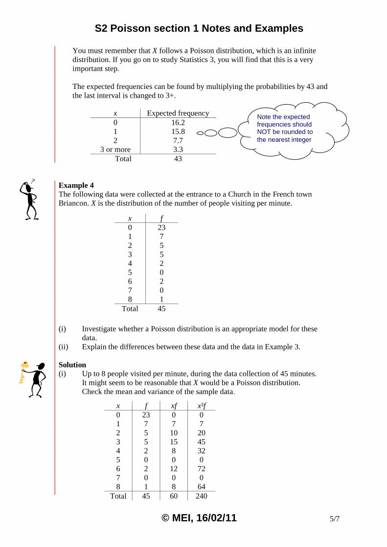
The expected frequencies can be found by multiplying the probabilities by 43 and

the last interval is changed to 3+.

Example 4

The following data were collected at the entrance to a Church in the French town

Briancon. X is the distribution of the number of people visiting per minute.

(i) Investigate whether a Poisson distribution is an appropriate model for these

data.

(ii) Explain the differences between these data and the data in Example 3.

Solution

(i) Up to 8 people visited per minute, during the data collection of 45 minutes.

It might seem to be reasonable that X would be a Poisson distribution.

Check the mean and variance of the sample data.

Note the expected frequencies should NOT be rounded to

the nearest integer

x Expected frequency

0 16.2

1 15.8

2 7.7

3 or more 3.3

Total 43

x f

0 23

1 7

2 5

3 5

4 2

5 0

6 2

7 0

8 1

Total 45

x f xf x²f

0 23 0 0

1 7 7 7

2 5 10 20

3 5 15 45

4 2 8 32

5 0 0 0

6 2 12 72

7 0 0 0

8 1 8 64

Total 45 60 240


© MEI, 16/02/11 6/7

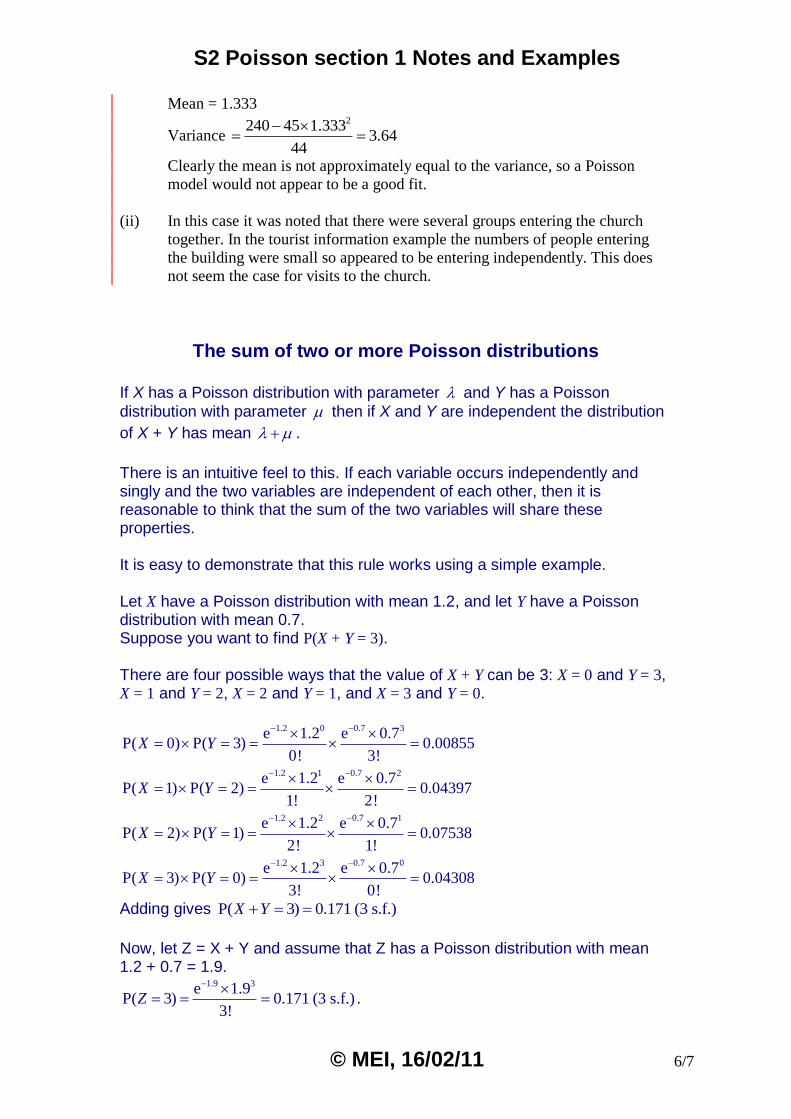
Mean = 1.333

Variance 2240 45 1.333

3.6444

Clearly the mean is not approximately equal to the variance, so a Poisson

model would not appear to be a good fit.

(ii) In this case it was noted that there were several groups entering the church

together. In the tourist information example the numbers of people entering

the building were small so appeared to be entering independently. This does

not seem the case for visits to the church.

The sum of two or more Poisson distributions

If X has a Poisson distribution with parameter and Y has a Poisson

distribution with parameter then if X and Y are independent the distribution

of X + Y has mean .

There is an intuitive feel to this. If each variable occurs independently and singly and the two variables are independent of each other, then it is reasonable to think that the sum of the two variables will share these properties. It is easy to demonstrate that this rule works using a simple example. Let X have a Poisson distribution with mean 1.2, and let Y have a Poisson distribution with mean 0.7. Suppose you want to find P(X + Y = 3). There are four possible ways that the value of X + Y can be 3: X = 0 and Y = 3, X = 1 and Y = 2, X = 2 and Y = 1, and X = 3 and Y = 0.

1.2 0 0.7 3

1.2 1 0.7 2

1.2 2 0.7 1

1.2 3 0.7 0

e 1.2 e 0.7P( 0) P( 3) 0.00855

0! 3!

e 1.2 e 0.7P( 1) P( 2) 0.04397

1! 2!

e 1.2 e 0.7P( 2) P( 1) 0.07538

2! 1!

e 1.2 e 0.7P( 3) P( 0) 0.04308

3! 0!

X Y

X Y

X Y

X Y

Adding gives P( 3) 0.171 (3 s.f.) X Y

Now, let Z = X + Y and assume that Z has a Poisson distribution with mean 1.2 + 0.7 = 1.9.

1.9 3e 1.9P( 3) 0.171 (3 s.f.)

3!

Z .


© MEI, 16/02/11 7/7

The two answers agree. Note that this does not prove the rule about the sum of two Poisson distributions, it just demonstrates that the rule works for a particular example. A proof is given in Appendix 2 (page 160) of the textbook. Using this rule does simplify considerably the calculations required. However, care must be observed in checking that the variables are independent. Example 5

On a fairly quiet road, on average 15 cars and 4 lorries or vans pass per 5 minutes.

Assuming that these are independent, find the probability that a total of 18 vehicles

pass in 5 minutes.

Solution

Without adding the 2 distributions together we would need to calculate:

P(18 cars) P(0 lorries or vans) + P(17cars) P(1 lorry or van) +

P (16 cars) P(2 lorries or vans) + P(15 cars) P(3 lorries or vans) +

P (14 cars) P(4 lorries or vans) + ….

Instead, combine the two distributions with, say, T: the distribution of cars and lorries

and vans.

So assuming that the distributions of cars and lorries and vans are independent then T

is Poisson with mean 19.

We require 19 18e 19

P( 18) 0.091118!

T

MEI Statistics 2

© MEI, 16/02/11 1/2

The Poisson Distribution

Section 2: The Poisson distribution as an approximation to

the Binomial distribution Notes and Examples These notes contain subsections on

Approximating the Binomial distribution

Approximating the Binomial distribution If X has a Binomial distribution with parameters n and p and if n is large and p is small then the distribution of X is closely approximated by a Poisson distribution with mean np. The approximation is very good for values of n larger than 50 and p smaller than 0.1.

The Autograph resource Poisson approximation to the binomial distribution compares the binomial distribution and its Poisson approximation graphically. Example 1

The discrete random variable X has a Binomial distribution with n = 70 and p = 0.05.

Determine the probabilities P(X = 0), P(X = 1)…. P(X = 5)

(i) using the exact distribution

(ii) using a Poisson distribution.

Solution

(i) 70 0 70

0P( 0) C (0.05) (0.95) 0.0276X

70 1 69

1P( 1) C (0.05) (0.95) 0.1016X

70 2 68

2P( 2) C (0.05) (0.95) 0.1845X

70 3 67

3P( 3) C (0.05) (0.95) 0.2201X

70 4 66

4P( 4) C (0.05) (0.95) 0.1941X

70 5 65

5P( 5) C (0.05) (0.95) 0.1348X

(ii) Using a Poisson approximation, take λ = 70 0.05 = 3.5

3.5 0e 3.5

P( 0) 0.03020!

X

3.5 1e 3.5

P( 1) 0.10561!

X


© MEI, 16/02/11 2/2

3.5 2e 3.5

P( 2) 0.18502!

X

3.5 3e 3.5

P( 3) 0.21583!

X

3.5 4e 3.5

P( 4) 0.18884!

X

3.5 5e 3.5

P( 5) 0.13225!

X

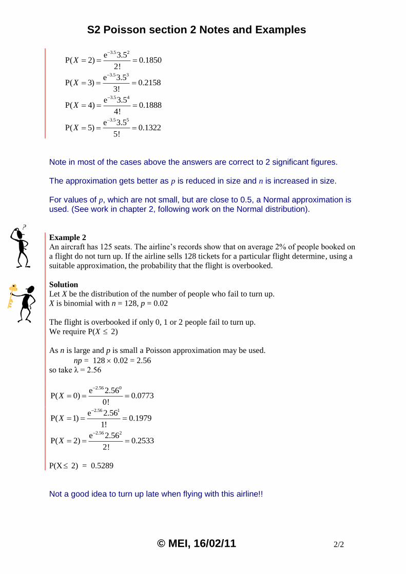
Note in most of the cases above the answers are correct to 2 significant figures. The approximation gets better as p is reduced in size and n is increased in size. For values of p, which are not small, but are close to 0.5, a Normal approximation is used. (See work in chapter 2, following work on the Normal distribution). Example 2

An aircraft has 125 seats. The airline’s records show that on average 2% of people booked on

a flight do not turn up. If the airline sells 128 tickets for a particular flight determine, using a

suitable approximation, the probability that the flight is overbooked.

Solution

Let X be the distribution of the number of people who fail to turn up.

X is binomial with n = 128, p = 0.02

The flight is overbooked if only 0, 1 or 2 people fail to turn up.

We require P(X 2)

As n is large and p is small a Poisson approximation may be used.

np = 128 0.02 = 2.56

so take λ = 2.56

2.56 0e 2.56

P( 0) 0.07730!

X

2.56 1e 2.56P( 1) 0.1979

1!X

2.56 2e 2.56P( 2) 0.2533

2!X

P(X 2) = 0.5289

Not a good idea to turn up late when flying with this airline!!

MEI Statistics 2

© MEI, 23/03/11 1/11

The Normal Distribution

Section 1: Introduction to the Normal distribution Notes and Examples These notes contain subsections on

The Normal curve

The standardised Normal distribution

Using inverse Normal tables

Non-standardised variables

Using inverse Normal tables for non-standardised variables

Further examples

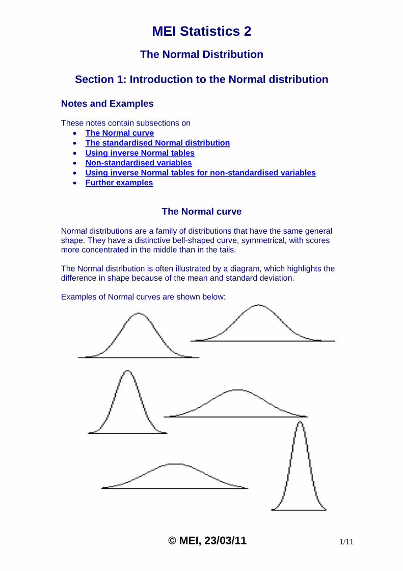
The Normal curve Normal distributions are a family of distributions that have the same general shape. They have a distinctive bell-shaped curve, symmetrical, with scores more concentrated in the middle than in the tails.

The Normal distribution is often illustrated by a diagram, which highlights the difference in shape because of the mean and standard deviation.

Examples of Normal curves are shown below:

MEI S2 Normal distribution sec. 1 Notes & Examples

© MEI, 23/03/11 2/11

The standard Normal distribution The standard normal distribution is a normal distribution with a mean of 0 and a standard deviation of 1. Z is used if a variable has a standard normal distribution. Page 34 of the textbook highlights how you can read off values for the standard normal table. Normal distributions can be transformed to standard normal distributions. You can use the Geogebra resource The Normal distribution to investigate Normal curves and their relationship with the standardised Normal curve. If the variable X has mean μ and standard deviation, then x, a particular value of X, is transformed into z by the formula:

x

z

Once you have standardised a normal variable the z score shows how many standard deviations above or below the mean a particular score is. For example, consider a student who scored 80 on a test with a mean of 60 and a standard deviation of 10. Converting the test scores to z scores, the value x becomes:

80 60

210

z

So, a z score of 2 means that the original score was 2 standard deviations above the mean.

Remember in S1 you defined outliers by looking at values more than 2 standard deviations from the mean. You will see why this definition is used later in this chapter. There are two styles of notation commonly use in statistics text books, P(Z < 2) or (2) . In the examples in this section both notations are used to avoid in any confusion. You should keep to the notation you have been introduced to. Example 1

Find

(i) P(Z > 1)

(ii) P(Z < -2)

(iii) P(-2 < Z < 1)

(iv) P(-2 < Z < 2)

http://davidmlane.com/hyperstat/A6929.html




© MEI, 23/03/11 3/11

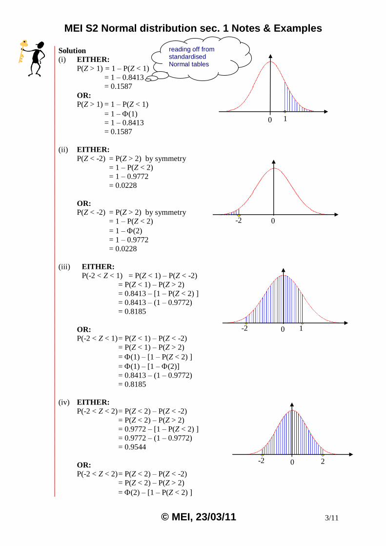
Solution

(i) EITHER:

P(Z > 1) = 1 – P(Z < 1)

= 1 – 0.8413

= 0.1587

OR:

P(Z > 1) = 1 – P(Z < 1)

= 1 – (1) = 1 – 0.8413

= 0.1587

(ii) EITHER:

P(Z < -2) = P(Z > 2) by symmetry

= 1 – P(Z < 2)

= 1 – 0.9772

= 0.0228

OR:

P(Z < -2) = P(Z > 2) by symmetry

= 1 – P(Z < 2)

= 1 – (2)

= 1 – 0.9772

= 0.0228

(iii) EITHER:

P(-2 < Z < 1) = P(Z < 1) – P(Z < -2) = P(Z < 1) – P(Z > 2)

= 0.8413 – [1 – P(Z < 2) ]

= 0.8413 – (1 – 0.9772)

= 0.8185

OR:

P(-2 < Z < 1) = P(Z < 1) – P(Z < -2)

= P(Z < 1) – P(Z > 2)

= (1) – [1 – P(Z < 2) ]

= (1) – [1 – (2)]

= 0.8413 – (1 – 0.9772)

= 0.8185

(iv) EITHER:

P(-2 < Z < 2) = P(Z < 2) – P(Z < -2)

= P(Z < 2) – P(Z > 2)

= 0.9772 – [1 – P(Z < 2) ]

= 0.9772 – (1 – 0.9772)

= 0.9544

OR:

P(-2 < Z < 2) = P(Z < 2) – P(Z < -2)

= P(Z < 2) – P(Z > 2)

= (2) – [1 – P(Z < 2) ]

1 -2 0

-2 0

0 1

reading off from standardised Normal tables

-2 0 2


© MEI, 23/03/11 4/11

= (2) – [1 – (2) ]

= 0.9772 – (1– 0.9772)

= 0.9544

In this last example you discovered that just over 95% of the values lie within 2 standard deviations from the mean for a standardised normal variable. You should remember from Statistics 1 that one definition of an outlier is any data item which is more than 2 standard deviations from the mean. For a set of data which can be modelled by the Normal distribution, this means that outliers are the most extreme 5% of the data. It is important that you understand how probabilities involving the standard normal distribution variable Z relate to an area under the standard normal curve. Try the Probabilities and Normal curves activity to help with this. Print out the whole file, and cut out all the rectangles. There are 12 rectangles which give a probability expression involving the standard normal distribution variable Z, 12 rectangles which give a numerical probability, and 12 copies of the standard Normal curve. You need to match up the probability expressions with the numerical probabilities, and also shade one of the Normal curves to show the area corresponding to this probability. There is also a more challenging version, in which you must match up

probability expressions with expressions involving the function, and again shade a Normal graph to show the appropriate area.

Using inverse Normal tables You will also need to be confident using the tables on the right hand side of page 34. Refer to page 42 to see how to use the diagram. Since the inverse Normal tables start with a probability of 0.5, you must always work with a probability of 0.5 or above. If you are given a probability of less than 0.5, you need to use symmetry:

P(Z < a) = p P(Z < -a) = 1 – p

Or, using the alternative notation:

(a) = p (-a) = 1 – p

Note that this is only true for a standard Normal distribution, since the mean is zero. Example 2 Version 1

Find a and b where:

(i) P(Z < a) = 0.845

(ii) P(Z < b) = 0.155


© MEI, 23/03/11 5/11

Solution Using the table on the right hand side of page 34, the Inverse Normal function:

(i) Looking up p = 0.845 gives z = 1.015

So a = 1.015

(ii) By symmetry P(Z < b) = 0.155 P(Z < -b) = 0.845 From part (i) you can see that -b = 1.015.

So b = -1.015

Example 2 Version 2 Find a and b where:

(i) (a) = 0.845

(ii) (b) = 0.155

Solution

Using the table on the right hand side of page 34, the Inverse Normal function:

(i) 1(0.845) 1.015a

(ii) By symmetry P(Z < b) = (b) = 0.155 (-b) = 0.845

1(0.845) 1.015b

So b = -1.015

Non-standardised variables Once you are confident using standardised normal variables you can apply the same techniques to other normal distributions by standardising the

variables using x

z

.

To convert from standardised scores to the value in its original context, you can use x z .

Example 3

If a test is normally distributed with a mean of 65 and a standard deviation of 10, what

proportion of the scores are above 85?

Solution 1

Let X be the distribution of test scores.

X ~ N (65, 102)

You require P(X > 85)

Now 85 65

10z

= 2

P(X > 85) = P(Z > 2)

= 1 – P(Z < 2)

= 1 – 0.9772

= 0.0228

x = 65

z = 0

x = 85

z = 2





© MEI, 23/03/11 6/11

Solution 2


X ~ N (65, 102)

You require P(X > 85)

Now 85 65

10z

= 2

P(X > 85) = P(Z > 2)

= 1 – P(Z < 2)

= 1 – (2) = 1 – 0.9772

= 0.0228

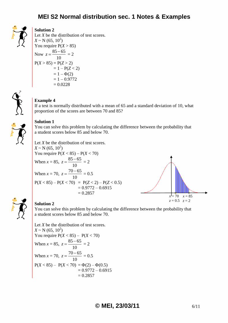
Example 4

If a test is normally distributed with a mean of 65 and a standard deviation of 10, what

proportion of the scores are between 70 and 85?

Solution 1 You can solve this problem by calculating the difference between the probability that

a student scores below 85 and below 70.


X ~ N (65, 102)

You require P(X < 85) – P(X < 70)

When x = 85, 85 65

10z

= 2

When x = 70, 70 65

10z

= 0.5

P(X < 85) – P(X < 70) = P(Z < 2) – P(Z < 0.5)

= 0.9772 – 0.6915

= 0.2857

Solution 2

You can solve this problem by calculating the difference between the probability that



X ~ N (65, 102)


When x = 85, 85 65

10z

= 2

When x = 70, 70 65

10z

= 0.5

P(X < 85) – P(X < 70) = (2) – (0.5)

= 0.9772 – 0.6915

= 0.2857

x = 70

z = 0.5

x = 85

z = 2





© MEI, 23/03/11 7/11

Example 5

Assume a test is normally distributed with a mean of 90 and a standard deviation of

15. What proportion of the scores would be between 75 and 95?

Solution 1




X ~ N (65, 102)


When x = 95, 95 90

15z

= 0.333

When x = 75, 75 90

15z

= -1

P(X < 95) – P(X < 75) = P(Z < 0.333) – P(Z < -1)

= 0.6304 – P(Z > 1)

= 0.6304 – [1 – P(Z < 1) ]

= 0.6304 – [1 – 0.8413 ]

= 0.4717

Solution 2




X ~ N (65, 102)


When x = 95, 95 90

15z

= 0.333

When x = 75, 75 90

15z

= -1

P(X < 95) – P(X < 75) = P(Z < 0.333) – P(Z < -1)

= (0.333) – P(Z > 1)

= 0.6304 – [1 – (1) ]

= 0.6304 – [1 – 0.8413 ]

= 0.4717

Using inverse normal tables for non-standardised variables You will also need to be confident using the tables on the right hand side of page 34, but be able to apply this knowledge to non-standardised variables. Remember that, as before, since the inverse Normal tables start with a probability of 0.5, you must always work with a probability of 0.5 or above. If you are given a probability of less than 0.5, you need to use symmetry:

P(Z < a) = p P(Z < -a) = 1 – p

x = 85

z = 0.333

x = 75

z = -1


© MEI, 23/03/11 8/11

Or, using the alternative notation:

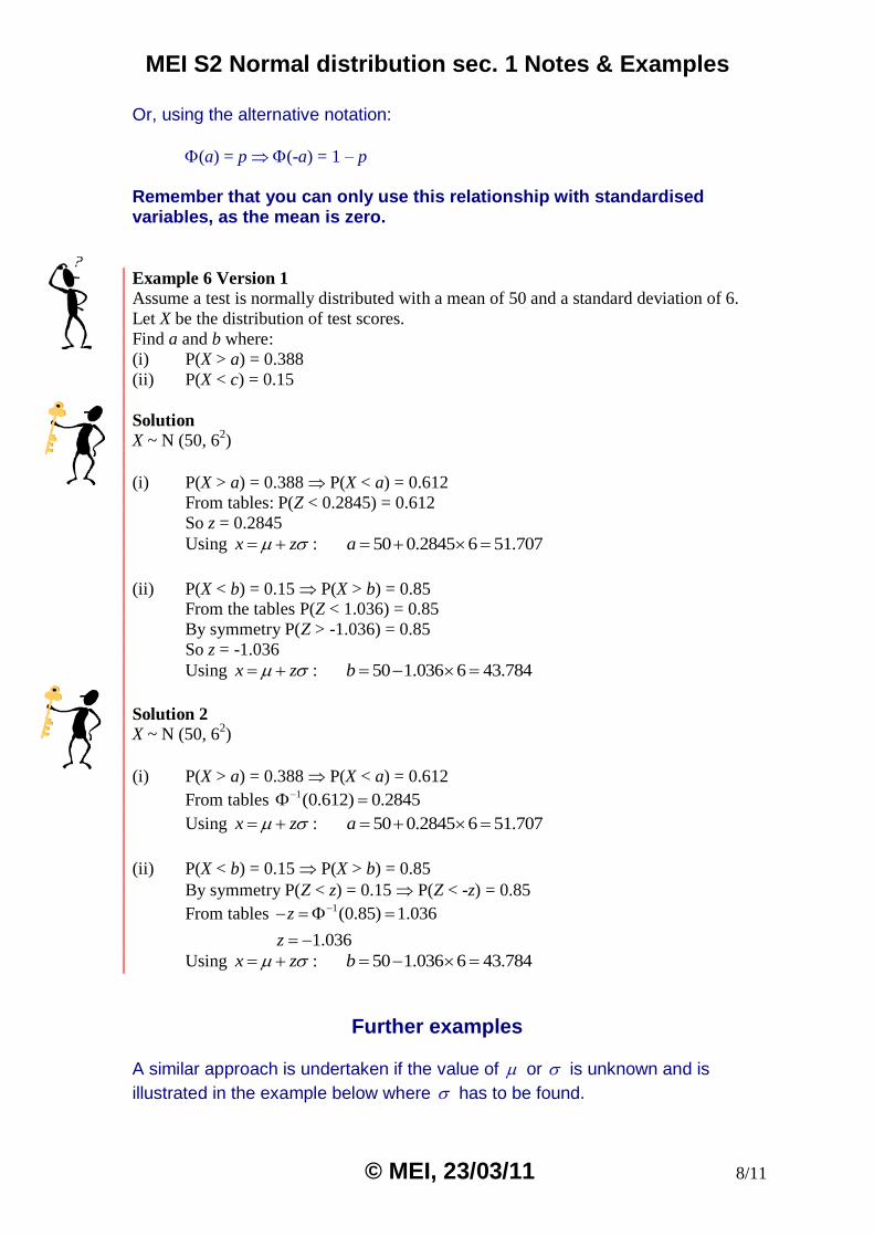
(a) = p (-a) = 1 – p Remember that you can only use this relationship with standardised variables, as the mean is zero. Example 6 Version 1

Assume a test is normally distributed with a mean of 50 and a standard deviation of 6.


Find a and b where:

(i) P(X > a) = 0.388

(ii) P(X < c) = 0.15

Solution

X ~ N (50, 62)

(i) P(X > a) = 0.388 P(X < a) = 0.612

From tables: P(Z < 0.2845) = 0.612

So z = 0.2845

Using x z : 50 0.2845 6 51.707 a

(ii) P(X < b) = 0.15 P(X > b) = 0.85 From the tables P(Z < 1.036) = 0.85

By symmetry P(Z > -1.036) = 0.85

So z = -1.036

Using x z : 50 1.036 6 43.784 b

Solution 2

X ~ N (50, 62)

(i) P(X > a) = 0.388 P(X < a) = 0.612

From tables 1(0.612) 0.2845

Using x z : 50 0.2845 6 51.707 a

(ii) P(X < b) = 0.15 P(X > b) = 0.85

By symmetry P(Z < z) = 0.15 P(Z < -z) = 0.85

From tables 1(0.85) 1.036

1.036

z

z

Using x z : 50 1.036 6 43.784 b

Further examples A similar approach is undertaken if the value of or is unknown and is

illustrated in the example below where has to be found.


© MEI, 23/03/11 9/11

Example 7

Assume a test is normally distributed with a mean of 50 and a standard deviation of

. Let X be the distribution of test scores.

Find if the probability of getting a score above 66 is 0.112.

Solution 1

X ~ N (50, 2)

Use the table on the right hand side of page 34, the Inverse Normal function.

The p table starts with a probability of 0.5. So we must always work with a

probability of 0.5 or above.

P(X > 66) = 0.112 P(X < 66) = 0.888

P(Z < 1.216) = 0.888

So z = 1.216

Now when x = 66, 66 50 16

z

161.216

= 16

13.161.216

Solution 2

X ~ N (50, 2)

We use the table on the right hand side of page 34, the Inverse Normal function.

The p table starts with a probability of 0.5. So we must always work with a

probability of 0.5 or above.

P(X > 66) = 0.112 P(X < 66) = 0.888 1( ) 0.888 (0.888) 1.216z z

Now when x = 66, 66 50 16

z

161.216

1613.16

1.216

The final example looks at determining the limits where a percentage of the distribution is expected to lie. Example 8

Consider a Normal variable with mean 70 and variance 25.

Find the limits within which the central 95% of the distribution lies.

Solution

X ~ N(70, 25)


© MEI, 23/03/11 10/11

Let the limits within which the central 95% of the

distribution lies be a and b, where a < b. If 95% of the

values lie within a and b, then 2.5% of the values lie

either side of a and b.

Use the table on the right hand side of page 34, the

Inverse Normal function.

P(X < b) = 0.975

From tables P(Z < 1.96) = 0.975 so z = 1.96

Now when x = b, 70

5

bz

701.96

5

b

b = 70 + 51.96 = 79.8

EITHER: Now a and b must be symmetrical about the mean, which is 70.

a = 70 – 51.96 = 60.2

OR: P(X < a) = 0.025

From tables P(Z < -1.96) = 0.025 so z = -1.96

Now when x = a 70

5

az

70

1.965

a

a = 70 – 51.96 = 60.2

Solution 2

X ~ N (70, 25)

Let the limits within which the central 95% of the distribution lies be a and b, where

a < b. If 95% of the values lie within a and b, then 2.5% of the values lie either side of

a and b.

We use the table on the right hand side of page 34, the Inverse Normal function.

P(X < b) = 0.975


Now when x = b 70

5

bz

701.96

5

b

b = 70 + 51.96 = 79.8

EITHER: Now a and b must be symmetrical about the mean, which is 70.

a = 70 – 51.96 = 60.2

OR: P(X < a) = 0.025


70 b a

95%

2.5% 2.5%


© MEI, 23/03/11 11/11

Now when x = a 70

5

az

70

1.965

a

a = 70 - 51.96 = 60.2

The above example illustrates the use of outliers in S1. We have calculated 70 1.96 5

which is approximately (2x Standard deviation).

So if the distribution can be reasonably well modelled by a Normal distribution we would expect 95% of the values to lie within 2 standard deviations from the mean. Hence the result used in S1. Similar results can be obtained for a central region of 99%, which will use p = 0.995 and gets a multiplying value of 2.576. Similar results can be obtained for a central region of 90%, which will use p = 0.95 and gets a multiplying value of 1.645. If you continue on to S3 you will use these values to get confidence intervals.

MEI Statistics 2

© MEI, 16/02/11 1/8

The Normal Distribution

Section 2: Approximating the Poisson and binomial distributions

Notes and Examples These notes contain subsections on

Approximating a discrete distribution

Approximating the Binomial distribution

Approximating the Poisson distribution

Approximating a discrete distribution In this section we will look at cases where we approximate a discrete distribution, which has a similar shape to a Normal distribution, by a Normal distribution. This situation occurs in test marks or Intelligence Quotient (IQ) scores. IQ scores follow a distribution that has a similar shape to a Normal distribution, despite the IQ scores being given as an integer. It is very important in these cases to read the information carefully so you are not confused with the continuous case of the Normal distribution. Obviously there will be a good fit, as although the data is discrete it is still likely to be very close to symmetrical. As we are now initially dealing with a discrete value there is clearly a difference between P(X < 100) and P(X 100) for IQ scores. The Normal variable is continuous so takes all values, not just the integer values. These problems can be overcome by using a continuity correction. The following table is useful to assist you in making these continuity corrections.

Discrete Variable Continuous Variable

P(X < 6) P(X < 5.5)

P(X 6) P(X < 6.5)

P(X > 6) P(X > 6.5)

P(X 6) P(X > 5.5)

P(X = 6) P(5.5 < X < 6.5)

P(3 < X < 6) P(3.5 < X < 5.5)

P(3 < X 6) P(3.5 < X 6.5)

P(3 X < 6) P(2.5 X < 5.5)

P(3 X < 6) P(2.5 X < 5.5)

S2 Normal distribution section 2 Notes and Examples

© MEI, 16/02/11 2/8

To help you understand how a continuity correction is used model a discrete distribution using a continuous distribution, try the Continuity Match activity. The following example will highlight the care that has to be taken. Example 1

IQ scores are given as an integer value, X.

Tests are designed so that the distribution of scores has a mean of 100 and a standard

deviation of 15.

Determine the probabilities:

(i) P(X < 120)

(ii) P(80 < X < 120)

Solution 1

Using a Normal approximation:

X ~ N (100, 225)

(i) We require P(X < 120)

Applying a continuity correction, this is P(X < 119.5)

Now 119.5 100

15z

= 1.3

P(Z < 1.3) = 0.9032

(ii) We require P(80 < X < 120)

Applying a continuity correction, this is P(80.5 < X < 119.5)

= P(X < 119.5) – P(X < 80.5)

When x = 119.5, 119.5 100

15z

= 1.3

When x = 80.5, 80.5 100

15z

= -1.3

P(X < 119.5) – P(X < 80.5) = P(Z < 1.3) – P(Z < -1.3)

= P(Z < 1.3) – P(Z > 1.3)

= P(Z < 1.3) – [1 – P(Z < 1.3)]

= 2 P(Z < 1.3) – 1

= 2 0.9032 – 1 = 0.8064

Solution 2


X ~ N (100, 225)



Now 119.5 100

15z

= 1.3

(1.3) = 0.9032


© MEI, 16/02/11 3/8

(ii) We require P(80 < X < 120)


= P(X < 119.5) – P(X < 80.5)

When x = 119.5, 119.5 100

15z

= 1.3

When x = 80.5, 80.5 100

15z

= -1.3

P(X < 119.5) – P(X < 80.5) = (1.3) – (-1.3)

= (1.3) – [1 – (1.3)]

= 2 (1.3) – 1

= 2 0.9032 – 1 = 0.8064

Approximating the Binomial distribution You will remember that if X has a Binomial distribution with parameters n and p and if n is large and p is small then the distribution of X is closely approximated by a Poisson distribution with mean np. In this section we will look at cases where we approximate the Binomial by a Normal distribution. You may use the Normal distribution as an approximation for the Binomial with parameters n and p when:

n is large

p is not small or large, i.e. close to 0.5. This seems logical. The Normal distribution is a symmetrical distribution so we will want the Binomial to have a similar shape. As n becomes larger the approximation is still good for values that are quite some way from p = 0.5. If X has a Binomial distribution with parameters n and p and if n is large and p is small then the distribution of X can be approximated by a Normal distribution with mean np and variance npq. However, we not only need to consider the parameters of the Normal distribution we must solve the problem of modelling a discrete distribution by a continuous distribution, as for the problem of IQ scores. This is again overcome by using a continuity correction. There is an obvious reason why we approximate a Binomial Distribution by a Normal Distribution. Up to now you have probably only calculated 2 or 3 Binomial probabilities in a question, or have used the Cumulative Probability Tables.


© MEI, 16/02/11 4/8

However, imagine a case where X is a Binomial variable with n = 100 and

p = 0.4. Imagine that you have to calculate P(X 60). Binomial tables do not go up to such a high value of n, so this would require 61 calculations! Instead you can do a Normal approximation and do one calculation!

The Autograph resource Normal approximation to the binomial distribution compares the binomial distribution and its Normal approximation graphically. Example 2

The discrete random variable X has a Binomial distribution with n = 100 and p = 0.4


(i) P(X < 50)

(ii) P(X > 50)

(iii) P(X 45)

(iv) P(X = 30)

by using a suitable approximation.

Solution 1


In this case np = 100 0.4 = 40

and npq = 100 0.4 0.6 = 24

X ~ N (40, 24)



Now 49.5 40

24z

= 1.939

P(Z < 1.939) = 0.9737

(ii) We require P(X > 50)

Applying a continuity correction, this is P(X > 50.5) = 1 – P(X < 50.5).

Now 50.5 40

24z

= 2.143

P(Z < 1.939) = 0.9839

P(X > 49.5) = 1 – P(X < 49.5) = 1 – 0.9839 = 0.0161

(iii) We require P(X 45) Applying a continuity correction, this is P(X < 45.5).

Now 45.5 40

24z

= 1.123

P(Z < 1.123) = 0.8690

(iv) We require P(X = 30)


= P(X < 30.5) – P(X < 29.5)


© MEI, 16/02/11 5/8

Now when x = 30.5,30.5 40

24z

= -1.939

and when x = 29.5 29.5 40

24z

= -2.143

P(X < 30.5) – P(X < 29.5) = P(Z < -1.939) – P(Z < -2.143)

= P(Z > 1.939) – P(Z > -2.143)

=[1 – P(Z < 1.939)] – [1 – P(Z < 2.143)]

=1 – 0.9737 – [1 – 0.9839]

= 0.0102

Solution 2

Using a Normal approximation: np = 100 0.4 = 40

and npq = 100 0.4 0.6 = 24

X ~ N (40, 24)



Now 49.5 40

24z

= 1.939

(1.939) = 0.9737

(ii) We require P(X > 50)

Applying a continuity correction, this is P(X > 50.5) = 1 – P(X < 50.5)

Now 50.5 40

24z

= 2.143

(2.143) = 0.9839

P(X > 49.5) = 1 – P(X < 49.5) = 1 – 0.9839 = 0.0161

(iii) We require P(X 45)


Now 45.5 40

24z

= 1.123

(1.123) = 0.8690

(iv) We require P(X = 30)


= P(X < 30.5) – P(X < 29.5)

Now when x = 30.5, 30.5 40

24z

= -1.939

and when x = 29.5, 29.5 40

24z

= -2.143

P(X < 30.5) – P(X < 29.5) = (-1.939) – (-2.143)

= [1 – (1.939)] – [1 – ( 2.143)] = 1 – 0.9737 – [1 – 0.9839]

= 0.0102


© MEI, 16/02/11 6/8

Approximating the Poisson distribution

In this section you will look at cases where you approximate the Poisson distribution by a Normal distribution. You may use the Normal distribution as an approximation for the Poisson distribution with parameter λ (λ is the mean) when λ is sufficiently large. The Normal distribution is a symmetrical distribution so you need the Poisson to be reasonably symmetrical. As λ becomes larger the approximation improves; it is useable for λ at 10 or larger. (Some textbooks suggest a value of 20 or more to get a higher degree of accuracy). The parameter λ is equal to the mean and the variance for a Poisson distribution, so for the Normal approximation we use X N(λ, λ) As with the Binomial approximation to a Normal distribution you must deal with the problem of modelling a discrete distribution by a continuous distribution. Remember that the Poisson variable will have values 0, 1, 2, 3, ….. The Normal variable is continuous so takes all values, not just the integer values. You can overcome these problems by using a continuity correction, as for the Binomial approximation. See the table produced for the Binomial approximation; the reasoning is exactly the same in this section. As we are now initially dealing with a discrete

value there is clearly a difference between P(X < 6) and P(X 6) for a Poisson variable. The following examples will highlight the care that has to be taken. As for the binomial, there is an obvious reason why we approximate a Poisson Distribution by a Normal Distribution. Up to now you have probably only calculated 2 or 3 Poisson probabilities in a question, or have used the Cumulative Probability Tables. However, imagine a case where X is a Poisson variable with λ = 70

Imagine that we have to calculate P(X 60). Since Poisson tables do not go

up to this value of , this would require 61 calculations! Instead you can do a Normal approximation and do one calculation!

The Autograph resource Normal approximation to the Poisson distribution compares the Poisson distribution and its Normal approximation graphically.


© MEI, 16/02/11 7/8

Example 3

The discrete random variable X has a Poisson distribution with λ = 30.


(i) P(X < 20)

(ii) P(X 15) (iii) P(X = 30)

by using a suitable approximation.

Solution 1


In this case = 30

X ~ N(30, 30)



Now 19.5 30

30z

= -1.917

P(Z < -1.917) = P(Z > 1.917) = 1 – P(Z < 1.917) = 1 – 0.9723 = 0.0277

(ii) We require P(X 15) Applying a continuity correction, this is P(X > 14.5) = 1 – P(X < 14.5)

Now 14.5 30

30z

= -2.830

P(Z < -2.830) = 1 – P(Z < 2.830) = 1 – 0.9977 = 0.0023

Use P(X > 14.5) = 1 – P(X < 14.5) = 1 – 0.0023 = 0.9977

(iii) We require P(X = 30)


= P(X < 30.5) – P(X < 29.5)

Now when x = 30.5 30.5 30

30z

= 0.091

and when x = 29.5 29.5 30

30z

= -0.091

P(X < 30.5) – P(X < 29.5) = P(Z < 0.091) – P(Z < -0.091)

= P(Z < 0.091) – P(Z > 0.091)

= P(Z < 0.091) – [1 – P(Z < 0.091)]

= 2 P(Z < 0.091) – 1

= 2 0.5363 –1

= 0.0726

Solution 2


In this case λ = 30

X ~ N (30, 30)



Now 19.5 30

30z

= -1.917


© MEI, 16/02/11 8/8

(-1.917) = 1 – (Z < 1.917) = 1 – 0.9723 = 0.0277

(ii) We require P(X 15) Applying a continuity correction, this is P(X > 14.5) = 1 – P(X < 14.5)

Now 14.5 30

30z

= -2.83

(-2.83) = 1 – (2.83) = 1 – 0.9977 = 0.0023

P(X > 14.5) = 1 – P(X < 14.5) = 1 – 0.0023 = 0.9977

(iii) We require P(X = 30)


= P(X < 30.5) – P(X < 29.5)

Now when x = 30.5, 30.5 30

30z

= 0.091

and when x = 29.5, 29.5 30

30z

= -0.091

P(X < 30.5) – P(X < 29.5) = (0.091) – (-0.091)

= (0.091) – [1 – (0.091)]

= 2 (0.091) – 1

= 2 0.5363 – 1

= 0.0726

To practise using approximating distributions and continuity corrections, try the Approximation Dominoes activity. Print out the dominoes and cut them out. Then match the right-hand side of each domino with a suitable approximating distribution on the left-hand side of another domino. This could be a Normal approximation to a binomial or Poisson distribution, or a Poisson approximation to a binomial distribution (covered in chapter 1). The dominoes should eventually form a closed loop.

MEI Statistics 2

© MEI, 14/03/11 1/13

Samples and Hypothesis Testing

Section 1: Hypothesis tests for the mean Notes and Examples These notes contain subsections on:

The distribution of sample means

Standardising the distribution of the sample means

Hypothesis tests

Using estimated standard deviation

The left-hand tail

Two-tailed tests

The distribution of sample means Suppose you use a random number generator to choose three numbers at random from the integers 1 – 100, and find the average of the three numbers you have chosen. There are a very large number of possible results you could obtain for the mean of your sample of three, ranging from 1 (if the numbers you obtain are all 1’s) to 100 (if the numbers you obtain are all 100’s). Clearly, it is quite unlikely that the mean would be 1 or 100 – it is much more likely to be fairly close to 50. You could work out the probability distribution for the sample means, by calculating the probability of each possible value for the mean. What sort of shape would this probability distribution have, and what would be the mean and standard deviation of the distribution? You can investigate the distribution of sample means using a simple example: throwing an ordinary, fair die. This means that you are dealing with the population {1, 2, 3, 4, 5, 6}. Throwing one die is equivalent to taking a sample of size 1 from the population; throwing two dice is equivalent to taking a sample of size 2 from the population, and so on. Samples of size 1 If you throw one die, then there are six possible samples you could obtain: {1} {2} {3} {4} {5} {6}

Each of these samples is equally likely to occur. The sample mean in each case is, of course, just the value of the score on the die. So the probability distribution of the sample means for a sample of size 1 is:

x 1 2 3 4 5 6

P( )X x 16

16

16

16

16

16

S2 Hypothesis testing section 1 Notes and Examples

© MEI, 14/03/11 2/13

0.05

0.1

0.15

0.2

x

p

1 1 1 1 1 16 6 6 6 6 6

E( ) 1 2 3 4 5 6

3.5

X

2 2 2 2 2 2 21 1 1 1 1 16 6 6 6 6 6

2916

3512

Var( ) 1 2 3 4 5 6 [E( )]

3.5

X X

Samples of size 2 If you throw two dice, then there are 36 possible samples you could obtain (some of which are the same, e.g. {1, 2} and {2, 1}). The table below shows the possible values of the sample mean.

1 2 3 4 5 6

1 1 1.5 2 2.5 3 3.5 2 1.5 2 2.5 3 3.5 4 3 2 2.5 3 3.5 4 4.5 4 2.5 3 3.5 4 4.5 5 5 3 3.5 4 4.5 5 5.5 6 3.5 4 4.5 5 5.5 6

So the probability distribution of the sample means for a sample of size 2 is: y 1 1.5 2 2.5 3 3.5 4 4.5 5 5.5 6

P( )Y y 136

236

336

436

536

636

536

436

336

236

136

0.05

0.1

0.15

0.2

x

p

3 5 6 51 2 436 36 36 36 36 36 36

34 2 136 36 36 36

E( ) 1 1.5 2 2.5 3 3.5 4

4.5 5 5.5 6

3.5

Y

2 2 2 2 2 2 23 5 6 51 2 436 36 36 36 36 36 36

2 2 2 2 234 2 136 36 36 36

3524

Var( ) 1 1.5 2 2.5 3 3.5 4

4.5 5 5.5 6 [E( )]

Y

Y


© MEI, 14/03/11 3/13

Samples of size 3 If you throw three dice, then there are 216 possible samples you could obtain (again, some are the same, such as {1, 1, 2}, {1, 2, 1} and {2, 1, 1}). If a complete list is made of all the possible samples, and the sample mean calculated for each, you can find the probability distribution of the sample mean in the same way as for samples of size 2. The probability distribution of the sample means for a sample of size 3 is:

z 1 13

1 23

1 2 13

2 23

2 3 13

3 23

3 4 13

4 23

4 5 13

5 23

5 6

P( )Z z 1216

3216

6216

10216

15216

21216

25216

27216

27216

25216

21216

15216

10216

6216

3216

1216

0.05

0.1

0.15

0.2

x

p

3 5 6 10 7 15 8 251 4 21216 3 216 3 216 216 3 216 3 216 216

10 27 27 25 13 15 1011 21 143 216 3 216 216 3 216 3 216 216

16 6 17 3 13 216 3 216 216

E( ) 1 2 3

4 5

6

3.5

Z

2 2 222 2 23 5 6 10 7 15 8 251 4 21216 3 216 3 216 216 3 216 3 216 216

2 22 22 210 27 27 25 13 15 1011 21 143 216 3 216 216 3 216 3 216 216

2 2 2 216 6 17 3 13 216 3 216 216

3536

Var( ) 1 2 3

4 5

6 [E( )]

Z

Z

Comparing the distributions for samples of size 1, 2 and 3, you can see that whereas a sample of size 1 has a uniform distribution, for samples of size 2 and 3 the distribution has a peak in the centre corresponding to the mean value of 3.5. In addition, the distribution for sample size 2 is triangular, whereas the one for sample size 3 is more “bell-shaped”, suggesting that the standard deviation is smaller. In fact, this trend continues with larger sample sizes. We have used the theoretical distribution of throwing a die to model the outcomes of sampling from a very simple population (the numbers 1, 2, 3, 4, 5

and 6). The mean (3.5) and standard deviation ( 3512

), calculated using the

random variable theory from Statistics 1 are the same as the population

mean, , and standard deviation, (the population standard deviation is calculated using divisor n, since we are dealing with a complete population).


© MEI, 14/03/11 4/13

All three probability distributions have mean 3.5, which is the same as the

population mean .

The standard deviation of the distribution for sample size 2 is 3524

, which can

be written as 2

. The standard deviation of the distribution for sample size 3

is 3536

, which can be written as 3

.

Generalising: given a population with a mean of μ and a standard deviation of σ, the sampling distribution of the mean has a mean of μ and a standard

deviation of

n, where n is the sample size.

Notice that the standard deviation of the distribution of sample means (sometimes called the standard error of the mean) is smaller than the population standard deviation and decreases as the sample size increases. As the distribution of the sample means is so important, it is often abbreviated to just the sampling distribution. However, this does not mean other sampling distributions are not possible: the sampling distribution of the median is possible of course. In this chapter we are assuming that the underlying distribution has a Normal distribution. Given a population X with a mean of μ and a standard deviation of σ i.e. X ~ N(μ , 2), and a sample of size n is taken, the distribution of the

sample means is given by X ~ N(μ , 2

n).

You can therefore use the skills learnt in the previous chapter to calculate probabilities with a sample mean. Note you can become confused between the theoretical distribution and a practical experiment. If you are conducting a biology experiment you will normally be collecting one sample of data. When analysing the results you are using the theory from the theoretical distribution.

Standardising the distribution of the sample means As you saw in chapter 2, normal distributions can be transformed to standard normal distributions. If the variable X has mean μ and standard deviation σ then x, a particular value of X, is transformed into z by the formula:

xz


© MEI, 14/03/11 5/13

So for the distribution of the sample means, X , you can standardise by using

xz

n.

There are two styles of notation commonly use in statistics text books,

P(Z < 2) or (2) . In the examples in this section both notation are used to avoid any confusion: keep to the notation you have been introduced to.

Hypothesis tests On pages 72 - 73 three different methods for carrying out a hypothesis test are shown. This may seem confusing, but in actual fact all three are really the same procedure, just approached in slightly different ways. You may feel that Method 2 seems familiar, as it is the same approach that you used for hypothesis tests involving the Binomial distribution in Statistics 1. We will start from Method 2, and show that the other two methods are equivalent. We will look at a general situation, similar to the one in Example 3.2. The null and alternative hypotheses are:

H0: = m

H1: > m

where is the true population mean. The significance level is p, which is given as a decimal, so that for a 5% significance level p would be 0.05. In Method 2, you need to look at the probability a sample of size n taken from

a distribution with mean m and standard deviation , has a value at least as extreme (in this case, at least as large) as x , the mean of the given sample. If

this probability is less than the significance level, p, you will reject H0. In such a case you are saying that it is so unlikely that a sample from a distribution with mean m would give us this value for x , that you conclude that in fact the distribution does not have mean m, but a larger mean.

The distribution of the sample means is N(m, ²

n).

Using Method 2, we say that we reject H0 if P ( ) X x p .

m x

)(P xX

The diagram shows a Normal distribution with mean m and

standard deviation . If the area shown is less than the significance level, we reject H0.


© MEI, 14/03/11 6/13

Now P ( ) X x p 1

x mp

n

1

x mp

n

1(1 )

x mp

n

x mk

n

where k is found from inverse normal tables. For a significance level of 5%,

k = -1

(0.95).

This is Method 3! H0 is rejected if

x mk

n, where k is found as shown

above. What you are actually doing here is finding the standardised Normal variable

x m

n (the test statistic) and comparing it with k, the critical value found from

the significance level.

Now

x mk

n

kx m

n

k

x mn

.

This is Method 1! We reject H0 if

k

x mn

, where k is found as shown

above.

0 k

Significance

level, p

This diagram shows a N(0, 1) distribution. Reject H0 if the test

statistic

x m

n lies to the right of k.

m

This is a N(m, ²)

distribution. c is the

critical value

k

mn

.

Reject H0 if x c .

c

Significance

level, p


© MEI, 14/03/11 7/13

You should be able to see that Methods 1 and 3 are very similar as they both involve comparison with a critical value. The difference is that in Method 3 you first standardise the sample mean, so that you can compare with a critical value for the N(0, 1) distribution. In Method 1 you work out the critical value

for the N(, ²) distribution, so that you can compare the sample mean with this. So which method should you use? Although Method 2 may seem familiar as you used a similar approach in Statistics 1, Methods 1 and 3 are more similar to other hypothesis testing in Statistics 2 and Statistics 3, in which you calculate a test statistic and compare this with a critical value. Method 3 is the standard method which most people use. However, you should also be familiar with the idea of finding a critical region (Method 1). The worked examples below show all three methods, but you are advised to concentrate on Method 3. This is the approach which is mostly used in the worked solutions on the website, and the answers in the textbook give the values of the test statistic. Note that the formula for the test statistic in Method 3 is given in the list of test statistics in your formula book (under Normal test for a mean).

Example 1

Test results for a module T1 are normally distributed with a mean of 65 and a

standard deviation of 10. After the introduction of a dynamic new teacher the results

for a group of 8 students had a mean of 72. Is there evidence that the results have

significantly improved at a 5% level of significance?

Solution H0 : μ = 65

H1 : μ > 65

where is the population mean test score.


X N(65, 102)

X N(65 , 210

8)

Method 1: Using critical regions

The critical value is given by

k

n.

The value of k is found from tables.

This is a one-tailed test at the 5% significance level:

P(Z < k) = 0.95

k = 1.645 OR: k =

-1(0.95)

k = 1.645

You want to see if the results could have come from a distribution where the population

mean has remained unchanged.

Remember to define as the population mean – there is often a mark awarded for this.





© MEI, 14/03/11 8/13

So the critical value is 1.645 10

65 70.88

Reject H0 for values of x greater than 70.8.

Since 72 > 70.8, the null hypothesis is rejected. There is evidence to suggest that the

mean score has increased, i.e. the teacher has had some effect.

Method 2: Using probabilities

We require P( X > 72)

Now 72 65

10 8

z = 1.980

P(Z > 1.980) = 1 – P(Z < 1.980)

= 1 – 0.9761

= 0.0239

OR P(Z > 1.980) = 1 – (1.980) = 1 – 0.9761

= 0.0239

Since 0.0239 < 0.05 (the required significance level of 5%) the null hypothesis is

rejected. There is evidence to suggest that the mean score has increased, i.e. the

teacher has had some effect.

Method 3: Using a standardised variable

The test statistic 72 65

10 8

z = 1.980

This is now compared with the critical value for z, which we get from tables.

5% significance level means that we are using:

P(Z < a) = 0.95

a = 1.645 OR: (a) = 0.95

a = 1.645

The test statistic 1.980 > 1.645

The null hypothesis is rejected. There is evidence to suggest that the mean score has

increased, i.e. the teacher has had some effect.

The Geogebra resource Hypothesis testing for the mean gives a graphical demonstration of the procedure for hypothesis testing for the mean. You can select the form of the alternative hypothesis and the significance level. A random sample from a Normal distribution is generated by pressing CTRL-R, and the test statistic, critical region and test result is shown.

Using estimated standard deviation The hypothesis test described above requires the value of the standard deviation of the parent population.

Statistics 2

© MEI, 14/11/05 9/13

In reality the standard deviation of the parent population will usually not be known. So in this case the standard deviation will have to be estimated from the sample data. In order for us to proceed with the same style of analysis we require the sample size to be sufficiently large. It is usual to require the sample size n to be 30 or above. Given a Normal population X with a mean of μ and unknown standard deviation, the sampling distribution of the mean is:

X N(μ, 2s

n)

where s2 is the estimated variance from the sample data. This is illustrated in the next example.

Example 2

The time taken for a bus to go from Oundle to Thrapston is normally distributed with

a mean time of 18 minutes. A new roundabout is introduced, which it is hoped will

speed up the journey.

A large number of observations are taken, following complaints from students that the

journey is now taking longer than 18 minutes.

From the 50 observations, the mean was found to be 19.1 minutes, with a sample

standard deviation of 5 minutes.

Investigate the students’ complaint, state a suitable null and alternative hypothesis for

the test and carry out the test at the 5% level of significance, stating your conclusion

carefully.

Solution

H0 : μ = 18.

H1 : μ > 18.

where is the population mean journey time.

Let X be the distribution of bus times.

We do not know the population variance, but as the sample size is large (n = 50) we

can estimate the distribution of the sample mean to be:

X N(18, 25

50)



k

n.



P(Z < k) = 0.95

k = 1.645 OR: k =

-1(0.95)

k = 1.645

Statistics 2

© MEI, 14/11/05 10/13


18 19.1650


Since 19.1 < 19.16, the null hypothesis is accepted. There is not sufficient evidence to

suggest that the journey time has increased. Students should stop moaning!


We require P( X > 19.3)

Now 19.1 18

5 50

z = 1.556

P(Z > 1.556) = 1 – P(Z < 1.556)

= 1 – 0.9401

= 0.0599

OR: P(Z > 1.556) = 1 – (1.556) = 1 – 0.9401

= 0.0599

Since 0.0599 > 0.05 (the required significance level of 5%) the null hypothesis is

accepted. There is not sufficient evidence to suggest that the journey time has

increased. Students should stop moaning!


The test statistic 19.1 18

5 50

z = 1.556



P(Z < a) = 0.95

a = 1.645 OR: (a) = 0.95

a = 1.645

The test statistic 1.556 < 1.645

The null hypothesis is accepted. There is not sufficient evidence to suggest that the

journey time has increased. Students should stop moaning!

The left-hand tail In the examples looked at so far, the critical region has been the right-hand tail of the distribution. In the next example, the critical region is the left-hand tail of the distribution. Example 3

The supplier of LITE light bulbs claims that the mean life of a LITE light bulb is 130

hours.

A training standards organisation tested 400 bulbs and found the mean to be 128.5

hours, with a sample standard deviation of 13 hours.

Is there evidence at a 2% level that the mean is lower than 130 hours?

Statistics 2

© MEI, 14/11/05 11/13

Solution

H0 : μ = 130

H1 : μ < 130.

where is the population mean lifetime.

Let X be the distribution of times of LITE light bulbs.

We do not know the population variance, but as the sample size is large (n = 400) we

can estimate the distribution of the sample mean to be:

X N(130, 213

400)


Since we are looking at the left-hand tail, the critical value is given by k

n

.



P(Z < k) = 0.98

k = 2.054 OR: k =

-1(0.98)

k = 2.054


130 128.66400

Since 128.5 < 128.66, the null hypothesis is rejected. There is evidence to suggest that

the lifespan of a LITE light bulb is less than 130 hours.


We require P( X < 128.5)

Now 128.5 130

13 400

z = -2.308

This time we are looking at the left-hand tail.

P(Z < -2.308 = 1 – P(Z < 2.308)

= 1 – 0.9895

= 0.0105

OR: (-2.308) = 1 – (2.308) = 1 – 0.9895

= 0.0105

Since 0.0105 < 0.02 (the required significance level of 2%) the null hypothesis is

rejected. There is evidence to suggest that that the lifespan of a LITE light bulb is less

than 130 hours.


We require P( X < 128.5)

Now 128.5 130

13 400

z = -2.308

Statistics 2

© MEI, 14/11/05 12/13



P(Z < a) = 0.98

a = 2.054 OR: a =

-1(0.98)

a = 2.054

This time we are looking at the left-hand tail so use a critical value of –2.054.

-2.308 < -2.054

The null hypothesis is rejected.

There is evidence to suggest that the lifespan of a LITE light bulb is less than 130

hours.

Two-tailed tests In all the examples so far, the alternative hypothesis has been of the form

> k (in which case you are looking at the right-hand tail) or < k (in which case you are looking at the left-hand tail). These are all one-tailed tests. However, sometimes you will need to look at situations where the alternative

hypothesis is of the form k (in which you are testing whether the mean is as stated or not, without specifying in which direction it is likely to be wrong. A test like this is a two-tailed test, as you are looking at both tails of the distribution. The next example looks at a two-tailed test. Example 4

The lengths of the leaves of a certain species of rare plant are Normally distributed

with mean 8.6 cm and standard deviation 1.2 cm. A botanist finds a clump of plants

and wants to find out whether they are of the rare species. She collects and measures

50 leaves and finds that the total of their lengths is 442 cm. Carry out a test at the 5%

level. What should the biologist conclude?

Solution

This is a two-tailed test, as the alternative hypothesis is that the mean is not 8.6, rather

than being specifically more or less than 8.6.

H0: = 8.6

H1: 8.6

where is the population mean leaf length.

84.850

442x

Let X be the distribution of the lengths of the leaves.

2.5%

2.5%

In this test, we are looking for evidence that the plants are

not of the rare species


© MEI, 15/06/09 13/13

X N(8.6, 21.2

50)

As the sample mean is greater than 8.6, we are looking at the right-hand tail.



k

n.


This is a two-tailed test at the 5% significance level:

P(Z < k) = 0.975

k = 1.960 OR: k =

-1(0.975)

k = 1.960

So the critical value is 1.960 1.2

8.6 8.932650


Since 8.84 < 8.9326, the null hypothesis is accepted. There is not sufficient evidence

to suggest that the plants are not of the rare species.


We require P( X > 8.84)

Now 8.84 8.6

1.41421.2 50

z

P(Z > 1.414) = 1 – P(Z < 1.414)

= 1 – 0.9213

= 0.0787

OR: P(Z > 1.556) = 1 – (1.414)

= 1 – 0.9213

= 0.0787

Since 0.0787 > 0.025 (the required significance level of 2.5% in each tail) the null

hypothesis is accepted. There is not sufficient evidence to suggest that the plants are

not of the rare species.


The test statistic 8.84 8.6

1.4141.2 50

z



P(Z < a) = 0.975

a = 1.960 OR: a =

-1(0.975)

a = 1.960

The test statistic 1.414 < 1.960

The null hypothesis is accepted. There is not sufficient evidence to suggest that the

plants are not of the rare species.

This is not the same as evidence that they are

of the rare species

MEI Statistics 2

© MEI, 15/06/09 1/5

Samples and Hypothesis testing

Section 2: Contingency Tables Notes and Examples These notes contain subsections on:

Hypothesis test for independence on contingency tables

The number of degrees of freedom

Hypothesis test for independence on contingency tables In this section we will look at cases where it is necessary to classify results according to two variables, where each variable can take two or more values. We wish to investigate if the two variables are independent. You will meet other ways of dealing with two variable data in chapter 4. A table is drawn up with one variable forming the rows and another variable forming the columns. There are many applications in other subject areas, psychology, geography or biology for example. For example you might want to investigate the growth of plants, which have been grown using different fertilisers and different soil conditions, or you could investigate the recall of male and female students under different conditions, such as a musical background or complete silence. In this section we will illustrate the method by an application in travel and tourism. Example 1

The marketing manager at a theme park and zoo undertakes a survey of a random

sample of 500 visitors. As part of this analysis he categorises them according to the

type of ticket they have bought.

Tickets are available for children, adults or Seniors.

There are four types of ticket available: Theme park only, zoo only, combined one-

day pass and combined two-day pass.

Note for this statistical analysis we do not need quantitative data for all or even any of the variables. However we do need some criteria in establishing which interval an observation should be placed.


© MEI, 15/06/09 2/5

The data is collected and inserted in a table.

The marketing manager wishes to see whether the two variables, distance travelled

and amount spent are related in any way.

(i) Carry out a hypothesis test to see if the two variables are independent.

(ii) Comment on the results.

Solution

(i) H0 : The age group and type of ticket are independent in the population

H1 : The age group and type of ticket are not independent in the population

Firstly add totals to the table.

Assume that the variables are independent.

Based on the totals, you would expect 54

500to have tickets for the zoo only and

193

500 to be children.

If independent, using S1 knowledge, we can multiply the probabilities:

P(child, zoo only) = 54 193

500 500

so in a sample of 500 the expected frequency for child, zoo only tickets would

be 54 193

500 20.844500 500

So for example 15 adults bought tickets for the zoo only A table with 4 rows and 3

columns is known as a 4 by 3 or 4 x 3 table.

Do not round!! Here we can keep the exact value. For a longer decimal, round to 2 d.p.

Observed

values

Age group

Child Adult Senior Total

Type of

ticket

Zoo 22 15 17 54

Theme park 45 39 26 110

Combined one-day 70 80 34 184

Combined two-day 56 78 18 152

Total 193 212 95 500

Age group

Child Adult Senior

Type of

ticket

Zoo 22 15 17

Theme park 45 39 26

Combined one-day 70 80 34

Combined two-day 56 78 18


© MEI, 15/06/09 3/5

Based on the totals, you would expect 54

500to have tickets for the zoo only and

212

500 to be adults.

P(adult, zoo only) = 54 212

500 500

so in a sample of 500 the expected frequency for adult, zoo only tickets would

be 54 212

500 22.896500 500

So any cell can be calculated by using Row total Column total

Sample size

.

We now need to compare the expected values with the observed values.

We label the expected frequencies as fe and the observed frequencies as fo

For each cell, calculate

2

o e

e

f f

f

and sum them up.

For Zoo and Child for example,

2 222 20.844

0.064120.844

o e

e

f f

f

Adding up these values gives 17.16.

This is the test statistic.

The number of degrees of freedom for an m by n table is given by

( 1) ( 1) m n (see explanation below). So in this case the number of degrees

of freedom is 3 2 6 .

Look up χ2 for six degrees of freedom. For a 5% significance level the critical

value is 12.59.

As you can see from the table in the formula book, the critical region is to the

right of the critical value.

The test statistic 17.16 > 12.59

2 values Age group

Child Adult Senior

Type of ticket

Zoo 0.0641 2.7230 4.4276

Theme park 0.1519 1.2515 1.2445

Combined one-day 0.1476 0.0505 0.0264

Combined two-day 0.1217 2.8497 4.0988

Expected

Values

Age group

Child Adult Senior

Type of ticket

Zoo 20.844 22.896 10.26

Theme park 42.46 46.64 20.9

Combined one-day 71.024 78.016 34.96

Combined two-day 58.672 64.448 28.88


© MEI, 15/06/09 4/5

In this case reject H0.

The evidence suggests that there is association between the two variables.

(ii) Looking at the table of ² values, the cells which make the largest

contributions to the value of the test statistics are the senior zoo and senior

two-day combined, followed by the adult zoo and adult two-day combined.

For all other cells, the ² values are quite small. There are less seniors and

more adults than would be expected with the two-day pass, and there are more

seniors and less adults than would be expected with the zoo only ticket.

Notice that large differences between the observed and expected values give rise to a large value of the test statistic. This is why H0 is rejected if the test statistic is larger than the critical value. Note that if there is some association between the two variables you cannot conclude that one variable causes an effect on the other. There could be a third variable involved.

The number of degrees of freedom The shape of the chi-squared distribution curve depends on the number of free variables involved, which is called the degrees of freedom and uses the

Greek letter (nu).

To find the value for you start off with the number of cells to be filled. You then subtract one degree of freedom for each restriction, derived from the data, which is put on the frequencies.

In the example covered above there were 4 3 boxes, i.e. a total of 12.

AMOUNT SPENT

Light Medium Heavy

Distance Travelled

Local 17 23 16

Medium 15 25 34

Long 4 16 12

Coach party 8 22 8

However, not all of these 12 boxes are independent because all the row and column totals have to be the same.

AMOUNT SPENT

Light Medium Heavy Total

Distance Travelled

Local 56

Medium 74

Long 32

Coach party

Total 44 86 70


© MEI, 15/06/09 5/5

There are 7 (4 + 3) totals but only 6 of these are independent. From these values in the table you can deduce the total is 200 and hence calculate the total for coach party. So there are 7 - 1 = 6 independent totals. In these rows and columns we only need a minimum of 6 filled cells in order to get all the cells filled. If you are given the following information:

AMOUNT SPENT


Distance Travelled

Local 25 30 56

Medium 8 31 74

Long 7 20 32

Coach party

Total 44 86 70

Then you can work out all the missing cells:

AMOUNT SPENT


Distance Travelled

Local 25 30 1 56

Medium 8 31 35 74

Long 7 20 5 32

Coach party 4 5 29 38

Total 44 86 70 200

So the number of degrees of freedom was 12 – (7 – 1) = 6

In general for a m n table (m rows and n columns)

Degrees of freedom is m n – (m + n – 1) = mn – m – n + 1 which factorises to (m – 1)(n – 1).

MEI Statistics 2

© MEI, 20/05/10 1/4

Bivariate data

Section 1: Product moment correlation Notes and Examples These notes contain subsections on

Scatter diagrams

The product moment correlation coefficient

Hypothesis tests involving the product moment correlation coefficient

Scatter diagrams You probably remember meeting scatter diagrams at GCSE level. You probably used them to gain a visual impression of whether there was any correlation in a set of bivariate data. You probably also drew lines of best fit by eye and may have used them to predict values. In this chapter you will learn to calculate correlation coefficients which measure the degree of correlation, and you will also learn (in section 3) to calculate the equation of the line of best fit for a set of bivariate data. You might therefore feel that the need for scatter diagrams is superseded by the use of calculated values. However, although the calculations you will learn in this chapter will give you more reliable information than the “by eye” methods you used at GCSE, scatter diagrams are still an important part of the process.

The scatter diagram allows you to spot any obvious outliers which may affect the results of your calculation.

You can see by the shape of the scatter diagram what procedures will be valid. For example, a hypothesis test using the product moment correlation coefficient is only a valid approach if both variables need to be drawn from a Normal distribution, indicated by an approximately elliptical shape. Alternatively, a scatter diagram may show non-linear correlation, in which case other methods may be used.

You can get some idea of the degree of correlation, and whether it is positive or negative, from the scatter diagram, which might allow you to spot if you have made an error in a calculation.

The product moment correlation coefficient You will find an explanation of Pearson’s product moment correlation coefficient, with the different methods of finding it, on pages 110 – 116 of your textbook. Look in particular at Example 4.1 on pages 112 – 114, and take

S2 Bivariate data Section 1 Notes and Examples

© MEI, 20/05/10 2/4

note of the two different methods used. Examination questions sometimes

give the summary statistics ( 2 2, , , , x x y y xy and n) rather than the

raw data (see Example 1 below), in which case you must use Method 2. If the data set is quite small and the numbers are not awkward, you may prefer Method 1. You are also shown in the textbook how to use a graphic calculator or spreadsheet to calculate the product moment correlation coefficient. These are useful approaches when dealing with large data sets. The Bivariate data interactive spreadsheet allows you to experiment with data and see how the value of the correlation coefficient relates to the scatter diagram. Select the first sheet (product moment). You can alter the position of the points, either by dragging the points on the scatter diagram, or by changing the values in the table of data, and see how the correlation coefficient changes. Try to arrange the data so that you have strong positive correlation, weak positive correlation, strong negative correlation and weak negative correlation. You could also try getting the correlation as close to zero as you can. You can also try the Geogebra resource Correlation and hypothesis testing, which can be used in a similar way to the spreadsheet. You can vary the number of points used on the scatter diagram. You can also try the product moment correlation coefficient activity, in which you match up scatter diagrams with values of the correlation coefficient.

Hypothesis test involving the product moment correlation coefficient

Make sure that you are aware of the following important points about this type of hypothesis test.

The test is only valid if the data are drawn from a Normal bivariate distribution, which is indicated by an approximately elliptical shape on a scatter diagram.

The calculation of the product moment correlation coefficient gives r, the sample product moment correlation coefficient. This is used as an

estimate for , the correlation coefficient for the parent distribution.

Your null and alternative hypotheses for the test involve , not r. The actual calculation of the product moment correlation coefficient and the comparison with the critical value from tables are fairly straightforward. However, it is possible to lose a number of easy marks in an exam by failing to include all the necessary commentary, using incorrect terminology and notation or by failing to draw the appropriate conclusion.


© MEI, 20/05/10 3/4

The steps in the hypothesis test should be as follows:

1. Write down the null and alternative hypotheses, using the symbol .

Include the definition of . 2. Write down the significance level. 3. Calculate the product moment correlation coefficient, r. 4. Look up the critical value from tables, stating the value of n, the

significance level and whether the test is one-tail or two-tail. 5. Compare (in writing) the value of r with the critical value. If the

magnitude of r is less than the critical value, then accept H0, if it is greater than the critical value, then reject H0.

6. State whether to accept or reject H0, and also write this conclusion in words in terms of the original problem, using language such as “Reject H0: there is evidence to suggest that there is (positive / negative) correlation between ....” or “Accept H0: there is not sufficient evidence to suggest that there is (positive / negative) correlation between ...”.

The spreadsheet Hypothesis test for correlation shows bivariate samples

taken from a bivariate normal distribution for which is approximately zero. You can set the sample size and the significance level, and the critical value for this case is given. When you press the Sample button, a sample of the appropriate size is taken and the value of r calculated and compared with the critical value. The null hypothesis (which is true) is either accepted or rejected. If you repeat the sampling process many times, you should find that the proportion of times the null hypothesis is rejected is approximately equal to the significance level. You can also use the Geogebra resource Correlation and hypothesis testing, which shows the result of a hypothesis test for a set of points which you can drag around. Example 1

A researcher wishes to find out if there is any connection between the length of time

young children spend using computers and their reading ability.

She collects data on 50 seven-year-olds, summarised below.

The number of hours spent using a computer during a particular week is denoted by x.

The score in a reading test is denoted by y.

222 x 2 1604 x 2892 y

2 179558 y 11846 xy

Carry out a hypothesis test at the 5% level to determine whether there is any

connection between time spent on computers and reading ability.

Solution

H0 : = 0

H1 : 0

where is the correlation coefficient for the parent population.

There may be a mark

allocated to this statement!


© MEI, 20/05/10 4/4

Significance level is 5%. 2

2 2 2221604 50 618.32

50

xxS x nx

2

2 2 2892179558 50 12284.72

50

yyS y ny

222 289211846 50 994.48

50 50 xyS xy nx y

994.480.3608

618.32 12284.72

xy

xx yy

Sr

S S

The critical value for a two-tail test at the 5% significance level for n = 50 is 0.2787.

Since 0.3608 > 0.2787, reject H0. There is evidence to suggest that there is correlation

between time spent using computers and reading ability.

Note the following important points about the example above.

The test is two-tailed (H1 is 0) because of the wording of the problem. The researcher might want to look at whether using a computer improves children’s reading ability (in which case the test

would be one-tailed, with alternative hypothesis > 0), or she might have wanted to investigate whether using a computer has a detrimental effect on children’s reading (again a one-tailed test, but this time with

alternative hypothesis < 0). As it is, she was investigating whether there is any correlation at all.

The correlation coefficient is negative. You need to disregard the sign of the correlation coefficient when comparing with the critical value.

The conclusion is that there is evidence to suggest a correlation between the two variables. It does not mean that using computers has a negative effect on a child’s reading ability. For example, it might be the case that children who read well spend less time on a computer because they enjoy reading books, or perhaps parents who spend time helping their children with reading may also be those who are more likely to restrict the time their children spend on the computer. Issues such as these are very complex, and all that the hypothesis test tells us is that there appears to be some connection between the two variables.

MEI Statistics 2

© MEI, 15/06/09 1/3

Bivariate data

Section 2: Rank correlation Notes and Examples These notes contain subsections on

Spearman’s rank correlation coefficient

Hypothesis test using rank correlation

Spearman’s rank correlation coefficient Rank correlation is obviously useful when the data is given in ranked form, as in the example about tomatoes on page 132. However, rank correlation can sometimes also be used when raw data is available but it is not possible to use the product moment correlation coefficient because the data is not from a bivariate Normal distribution. For example, look back at Figure 4.16 on page 124, which show non-linear association. It would not be appropriate to use the product moment correlation coefficient in either of these cases. Spearman’s rank correlation coefficient would give a high degree of association for the data in the first diagram, although not for the data in the second diagram (can you see why? Think about assigning a rank to each item of data for the vertical and horizontal variables). If you want to know whether it is reasonable to assume that a sample is drawn from a bivariate Normal distribution, you can draw a scatter diagram. If the points form an elliptical pattern, then it is reasonable to assume that the population is bivariate Normal. You can also use common sense reasoning as to whether you would expect the distribution to be bivariate Normal, from the nature of the data. For example, suppose you wanted to investigate any association between the number of children in a household and the number of pets. For the underlying population to be bivariate Normal, then if you consider all households with no children, the number of pets should be Normally distributed; if you consider all households with one child, the number of pets should be Normally distributed; and so on. Similarly, if you consider all households with no pets, the number of children should be Normally distributed, and so on. Clearly this is unlikely. If raw data is given and is from a bivariate Normal distribution, then it is possible to use either the product moment correlation coefficient or Spearman’s rank correlation coefficient. In such cases it would normally be best to use the product moment correlation coefficient as this uses the actual values of the data and so gives a more accurate measure.


© MEI, 15/06/09 2/3

To use Spearman’s rank correlation coefficient, the data must be a random sample. The Bivariate data interactive spreadsheet allows you to experiment with data and see how the value of Spearman’s rank correlation coefficient relates to the scatter diagram. Select the second sheet (Spearman’s rank). You can alter the position of the points, either by dragging the points on the scatter diagram, or by changing the values in the table of data, and see how the correlation coefficient changes. Try to arrange the data so that you have strong positive association, weak positive association, strong negative association and weak negative association. You could also try getting the correlation as close to zero as you can. Can you get a value of 1 without having the data in a straight line?

Hypothesis test using rank correlation A hypothesis test using rank correlation is carried out in exactly the same way as the test using the product moment correlation coefficient, except that of course you are calculating a different correlation coefficient, and using a different set of tables for the critical values. However, there is an important difference in the way that you should state your hypotheses. It is not appropriate to use the word “correlation” or the

variable here, since these are associated with linear correlation (which is tested using the product moment correlation coefficient, as in section 1). Instead, the word “association” is used – you can also talk about “positive association” or “negative association” if you are using a one-tailed test. The correct form of the hypotheses is

H0: there is no association between ..... in the underlying population H1: there is an association between ..... in the underlying population

(for a two-tailed test) or H0: there is no association between ..... in the underlying population

H1: there is a positive association between ..... in the underlying population

or H0: there is no association between ..... in the underlying population

H1: there is a negative association between ..... in the underlying population

(for a one-tailed test) As for tests involving the product moment correlation coefficient, you must also be careful to make sure that you gain all the available marks for stating your conclusion, both as “accept / reject H0” and in terms of the original


© MEI, 15/06/09 3/3

problem. e.g. Accept H0: there is not sufficient evidence to suggest an association between ..... or Reject H0: there is evidence to suggest an association between.....

MEI Statistics 2

© MEI, 21/04/10 1/3

Bivariate data

Section 3: The least squares regression line Notes and Examples These notes contain subsections on

The least squares regression line

Using regression lines for predictions

Residuals

The least squares regression line If there is a linear connection between two sets of data, it may be appropriate to draw a line of best fit which can sometimes be used for predicting values. At GCSE level you may have drawn lines of best fit by eye: this is not very satisfactory as it may be difficult to judge which of the possible lines is the best. If several people all draw lines of best fit for the same data set by eye, and then find their equations, they may be quite different, even if they all look fairly convincing when drawn! In this section you learn to calculate the equation of the line of best fit (the least squares regression line, or the regression line for y on x). This is the line for which the sum of the squares of the residuals (the vertical distances of each point from the line) is as small as possible. Pages 142 – 143, together with Appendix 4, give the details which justify the formula for the regression line. There are several different ways in which the equation of the regression line may be written: the simplest is given at the foot of page 143, and is also given in similar form in your formula book:

( )y y b x x , where xy

xx

Sb

S .

Try the Regression matching activity, in which you match up scatter diagrams with the equation of a regression line.

Using regression lines for predictions A regression line may sometimes be used for predicting values, but you must be careful to consider whether or not this is appropriate. Firstly, you need to think about how good the linear model is for the data. This can often be judged from a scatter diagram:

it may be that the data does not really look linear

MEI S2 Bivariate data Section 3 Notes and Examples

© MEI, 21/04/10 2/3

the line might look like a good model within part of the range of the data but not for other parts of the range

You may need to extrapolate a graph in order to make a prediction. This may or may not be appropriate: you must think about the context. Look back to page 125 of the textbook which shows an example in which extrapolation is definitely inappropriate! It is important to be aware that you can only use a y on x regression line to make predictions for values of y. To make predictions for values of x, you would need to use the x on y regression line (in which the residuals are horizontal - this is not required by the syllabus). In many “real-life” situations, it is only possible to calculate one regression line because one of the variables is usually “controlled” (i.e. is not random) – for example, if measurements are taken at 10 second intervals, then the variable “time” is not random. However, if both variables are random, then both regression lines can be calculated and predictions made for both variables using the appropriate regression line. For now, however, you only need to be able to calculate the y on x regression line and to use it where appropriate to make predictions for y.

Residuals As mentioned before, the residual for each data point is the vertical distance between the point and the regression line. The sum of all the residuals is zero, but the sum of the squares of the residuals is used as a measure of how close the points are to the regression line.

These data look as if they fit a curve rather than a line, so the regression line will not give very

reliable predictions

The line is a very good fit up to about

x = 2.5, so for values of x between 0

and 2.5 the regression line could be

used to make predictions. However

for larger values of x the model looks

less appropriate, so predictions

become unreliable.

MEI S2 Bivariate data Section 3 Notes and Examples

© MEI, 21/04/10 3/3

It is important to realise that amongst all possible straight lines, the regression line is the one which minimises the sum of the squares of the residuals. You may be asked in an examination about the significance of the residuals. The Bivariate data interactive spreadsheet demonstrates that the sum of the squares of the residuals is minimised by the regression line. The regression line is initially shown on the spreadsheet. You can vary the

gradient of the line (which always passes through ,x y ) and you will see that

the sum of the squares of the residuals is at a minimum for the regression line. You can also change the data values if you wish. You can also try the Geogebra resource Regression, which can be used in a similar way.

mei statistics 2 - woodhouse...

Documents