Medium Term Business Cycles in Developing Countries1

Diego Comin†, Norman Loayza‡, Farooq Pasha♦ and Luis Serven‡2

First Version: October, 2009

This Version: October, 2013

1For excellent research assistance, we are grateful to Freddy Rojas, Naotaka Sugawara, and Tomoko

Wada. We have benefitted from insightful comments from Susanto Basu, Ariel Burnstein, Anto-

nio Fatás, Fabio Ghironi, Gita Gopinath, Aart Kraay, Marti Mestieri, Claudio Raddatz, Stephanie

Schmidt-Grohe, Akos Valentinyi, Lou Wells, and seminar participants at Harvard University, Bocconi,

Brown University, Carnegie Mellon, Harvard Business School, CEPR-Budapest, CEPR-Paris, HEC,

INSEAD, Boston College, EIEF, University of Milano Bicocca, and the World Bank. We gratefully

recognize the financial support from the Knowledge for Change Program of the World Bank. Comin

thanks the financial support by the National Science Foundation. The views expressed in this paper

are those of the authors, and do not necessarily reflect those of the institutions to which they are

affi liated.2†Harvard University, NBER and CEPR, ‡ The World Bank, ♦ Boston College.

Abstract

Business cycle fluctuations in developed economies (N) tend to have large and persistent effects

on developing countries (S). We study the transmission of business cycle fluctuations for

developed to developing economies with a two-country asymmetric DSGE model with two

features: (i) endogenous and slow diffusion of technologies from the developed to the developing

country, and (ii) adjustment costs to investment flows. Consistent with the model we observe

that the flow of technologies from N to S co-moves positively with output in both N and

S. After calibrating the model to Mexico and the U.S., it can explain the following stylized

facts: (i) shocks to N have a large effect on S; (ii) business cycles in N lead over medium term

fluctuations in S; (iii) the outputs in S and N co-move more than their consumption; and (iv)

interest rates in S are counter-cyclical .

Keywords: Business Cycles in Developing Countries, Co-movement between Developed and

Developing economies, Volatility, Extensive Margin of Trade, Product Life Cycle, FDI.

JEL Classification: E3, O3.

"Poor Mexico! So far from God and so close to the United States." Attributed to

Dictator Porfirio Diaz, 1910.

This paper explores the transmission of business cycle fluctuations for developed to develop-

ing economies. Business cycle fluctuations in developed economies tend to have strong effects

on developing countries. When studying more generally the co-movement patterns, we observe

evidence that the effects of business cycles in developed economies (N) on developing (S) ones

are not only large but also quite persistent. In particular, they affect output in developing

countries over the medium term and not only at business cycle frequencies.

A natural channel for the transmission of shocks from N to S is through N’s demand for

S ′ exports. Below we show, however, that this mechanism is unable to propagate shocks to

S with the persistence we observe in the data. We explore a different channel: the cyclicality

of the speed of diffusion of new technologies embodied in new capital goods from N to S.

Following Broda and Weinstein (2006), we measure technology diffusion by the number of

different (durable-manufacturing) SIC categories in which N exports to S. We uncover two

main facts. First, the number of technologies exported from N to S co-moves positively with

N ′s cycle, both at high frequency and at lower frequencies. Second, at low frequencies, the

range of technologies imported from N leads S productivity measures.

To explore the quantitative implications of these regularities for business cycles in developing

economies, we build a real business cycle model. Our model has two asymmetric countries with

endogenous productivity growth. In the North, R&D investments lead to the creation of new

technologies and to productivity growth (e.g., Comin and Gertler, 2006). In the South, instead,

productivity growth is linked to the transfer of new technologies from the North (i.e., technology

diffusion). It is well known (e.g. Comin and Hobijn, 2010) that developing countries adopt new

technologies with significant time lags relative to their invention date. In our model, exporters

from N need to incur a sunk cost before starting to sell the intermediate goods that embody

the technology in S. This sunk cost of exporting generates the adoption lag observed in the

data. To close the lifecycle of intermediate goods, we allow firms to transfer the production

of the intermediate goods to S after engaging in another sunk investment (i.e., foreign direct

investment). This allows us to capture realistically the nature of capital flows to developing

countries, of which, since 1990, 70% have been in the form of FDI (e.g., Loayza and Serven,

2006).1

1The FDI share is even larger when restricting attention to private capital flows and when focusing in Latin

1

As it is clear from this description, our framework is related to the product-cycle literature

(e.g., Stokey, 1991). The main theoretical contribution of our model is that it provides a unified

account of the dynamics of productivity over high and low frequencies in N and S. As in the

neoclassical model, the drop in current aggregate demand or productivity leads to a current

collapse in investment and output in S. However, in addition, adoption lags vary endogenously

with the cycle in our model. Contractionary shocks to either N or S reduce the present

discounted value of transferring a new technology to S, inducing pro-cyclical fluctuations in the

speed of technology diffusion. Because technology is a state variable and changes slowly, the

fluctuations in S ′ stock of technologies occur only at low frequencies. However, a few years into

the recession, productivity in S will have declined very significantly. As a result, the marginal

product of capital will still be very low and investment will have not recovered. The effect of

these extra state variables, is what allows our model to generate a hump-shaped response of S ′

investment and output to a recessionary shock in N.

In section 4, we calibrate the model to match basic (steady state) moments of the U.S.

and Mexican economies. The simulations show that our model does a reasonably good job in

characterizing the key features of the short and medium term fluctuations in Mexico. In doing

so, it sheds light on several important open questions in international macroeconomics.

First, unlike many RBCmodels (e.g. Backus, Kehoe and Kydland, 1992) our model generates

a higher cross-country correlation of output than that of consumption. It does so because

what drives the short term cross-country co-movement in output is the pro-cyclical response

of Mexico’s investment to U.S. shocks. Mexico’s consumption, on the other hand, does not

respond much contemporaneously to U.S. shocks. Second, our model also generates a large

initial response of S GDP to N shocks, which helps explain why business cycle fluctuations

are larger in developing than in developed economies. Third, consistent with the data, short

term fluctuations in N produce cycles in S at frequencies lower than those of the conventional

business cycle. This occurs because shocks in N triggers a persistent slowdown in the flow of

new technologies to S.

Fourth, the model generates counter-cyclical interest rates in S endogenously in response to

domestic shocks. As shown by Neumeyer and Perri (2005), an important feature of business

cycles in developing countries is the counter-cyclicality of real interest rates. Based on this

evidence, numerous authors have used shocks to interest rates in developing countries as a

source of business cycles. In our model, the procyclical diffusion of technologies generates

America and Asia.

2

counter-cyclical fluctuations in the relative price of capital. These result in counter-cyclical

capital gains from holding a unit of capital that dominate the pro-cyclical response of the

marginal product of capital (i.e. the dividend), thus inducing interest rates in S (as well as the

interest differential with respect to N) to be counter-cyclical.

The endogenous international diffusion of technologies emphasized in our framework is a

different phenomenon from production sharing (e.g. Bergin et al. 2009; Zlate, 2010). Pro-

duction sharing models generate large fluctuations in output in S in response to a shock in N

by assuming strong cyclicality of wages.2 Firms in N compare wages domestically and abroad

and expand and contract their offshoring arrangements by increasing the extent of traded in-

termediates. An implication of these models is that the flow of intermediate exports from N

to S should be pro-cyclical with respect to N ′s cycle but counter-cyclical with respect to S.

In contrast, in our framework both recessions in N and S reduce the present discounted value

of future profits from exporting a new intermediate good to S. As a result, the flow of new

technologies from N to S is pro-cyclical with respect to both countries, and in particular to

S. The data examined here shows strong evidence of the pro-cyclicality of the flow of new

technologies with respect to S.3 A related issue is that it is unlikely that production-sharing

models or models of entry and trade in varieties (e.g. Ghironi and Melitz, 2005) can account for

the low-frequency effects of N ′s business cycle on S ′s productivity and output we observe in the

data.4 The key conceptual difference with these models is that, in ours, investment decisions in

international technology transfer involve sunk costs, while in the literature they are fixed costs.

As a result, our mechanisms introduce new state variables that can generate the low-frequency

international propagation that characterizes the data.

The rest of the paper is organized as follows. The next section presents some basic stylized

facts. Section 3 develops the model. Section 4 evaluates the model through some simulations

2Another important assumption of production sharing models, though more plausible, is that the share of

manufacturing is larger in S than in N.3A different approach to modeling production sharing is followed by Burnstein, Kurz and Tesar (2008).

Rather than using variation in the extensive margin, their model assumes a complementarity between domestic

and foreign intermediate goods in U.S. production. By changing the importance of the sector where domestic

and foreign intermediate goods are complementary, they can generate a significant increase in the correlation

between U.S. and Mexican manufacturing output.4As we show in section 5, a key difference with trade in variety models is that the costs of affecting the

extensive margin are fixed but not sunk. Modeling the transfer of technology as a sunk investment introduces

a new state variable that changes the propagation and amplification of the shocks very significantly.

3

and provides intuition about the role of the different mechanisms. Section 5 discusses the results

and compares them to the literature, and section 6 concludes.

1 The cyclicality of international technology diffusion

In this section, we explore the role of technology diffusion in the propagation of business cy-

cles from developed (N) to developing (S) countries. We focus on the two largest developed

economies as N -countries: the U.S. and Japan.5 We then select the S-countries based on the

concentration of their (durable goods) imports from N .6 That is, for each developing country

without missing data and with a population of more than 2 million people, we construct an

index of concentration of imports from each of the two N -countries. The index is just equal to

the durable manufacturing imports from N over total imports of durable manufacturing. For

each country N, we select the 10 developing countries with the highest concentration.7

We collect data on three variables. First GDP per working age person as a measure of output

both in N and S. Next, following Greenwood and Yorukoglu (1997) and Greenwood, Hercowitz

and Krusell (1997), we measure the level of embodied productivity by ratio of the GDP deflator

over the investment deflator. Finally, following Broda and Weinstein (2006), we measure the

range of technologies that diffuse internationally from N to S by the number of 6-digit SIC

codes within durable manufacturing that have exports from N to S that are worth at least $1

million.

Our data are annual and cover the period 1960-2008. We use the full sample period to obtain

the filtered series. However, as we explain below, we focus our analysis on the period 1990-2008.

Because we want to allow for the possibility that shocks to N have a very persistent effect in

S, we analyze fluctuations at medium term frequencies in addition to conventional business

cycles. Following Comin and Gertler (2006), we define the medium term cycle as fluctuations

with periods smaller than 50 years. The medium term cycle can be decomposed into a high

5We do not include the EU because it has a lower syncronization of the business cycles betwen its members

than U.S. states or Japanese prefactures.6The emphasis on durable manufacturing goods is driven by the model and because durable manufacturing

goods surely embody more productive technologies than the average non-durable good. Having said that, the

list of developing countries would be very similar if we ranked countries by concentration in imports or trade.7The developing countries linked to the U.S. are Mexico, Dominican Republic, Costa Rica, Paraguay, Hon-

duras, Guatemala, Venezuela, Peru, El Salvador and Nicaragua. The countries linked to Japan are Panama,

Thailand, South Korea, Philippines, Vietnam, China, Pakistan, Indonesia, South Africa and Malaysia.

4

frequency component and a medium term component. The high frequency component captures

fluctuations with periods smaller than 8 years while the medium term component captures

fluctuations with periods between 8 and 50 years. We use a Hodrick-Prescott filter to isolate

fluctuations at the high frequency.8 We isolate the medium term component and the medium

term cycle using a band pass filter.

Two points are worth keeping in mind. First, it is important to be careful about the mapping

between the frequency domain and the time domain. In principle, our measure of the cycle

includes frequencies up to 50 years. However, Comin and Gertler (2006) have shown that

its representation in the time domain leads to cycles on the order of a decade, reflecting the

distribution of the mass of the filtered data over the frequency domain. For example, in the

U.S. postwar period there are ten peaks and throughs in the medium term component of the

cycle.9 Second, despite their frequency, medium term cycles identified with macro series of

conventional length are statistically significant (Comin and Gertler, 2006). We investigate the

significance of the medium term component of per capita income in the countries in our sample

by constructing confidence intervals using a bootstrap procedure.10 We find that 52% of annual

observations of the filtered series are statistically significant at 95% level. By way of comparison,

we find that 80% of the HP-filtered annual observations are significant. Therefore, we consider

that inferences based on series filtered to isolate medium term fluctuations are statistically

informative.

After filtering the macro variables, we study their co-movement patterns during the period

1990-2008. We focus on this period for two reasons. First, the volume of trade and FDI inflows

to developing countries increased very significantly during this period, making the mechanisms

emphasized by our model more relevant than before. Second, after 1990, FDI became the

most significant source of capital inflows from developed to developing economies, making our

model’s assumptions about the nature of international capital flows most appropriate for this

period (Loayza and Serven, 2006). To show how much the international co-movement changed,

we also present some results for the period 1975-90.

8The HP-filtered series are very similar to the series that result from using a Band-Pass filter that keeps

fluctuations with periodicity smaller than eight years (Comin and Gertler, 2006). We use the HP filter to isolate

high-frequency fluctuations to make our findings more comparable to the literature.9There are 22 peaks and throughs at conventional frequencies.10Specifically, we use the bootsrap method described in Comin and Gertler (2006). Essentially, the method

consists in padding the time series at both ends, and filtering the extended series. Then, for each period in the

original series, we build a 95% confidence interval.

5

Before analyzing the data, an example can be useful to illustrate the co-movement patterns

between developed and developing countries. Figure 1A plots the series of HP-filtered GDP in

the U.S. and Mexico. The contemporaneous cross-country correlation is 0.42 (with a p-value

of 7%). U.S. business fluctuations such as the internet-driven expansion during the second half

of the 1990s, the burst of the dot-com bubble in 2001, the 2002-2007 expansion and the 2008

financial crisis are accompanied by similar fluctuations in Mexico. Arguably, none of the shocks

that caused these U.S. fluctuations originated in Mexico. Therefore, it is natural to think that

the co-movement between Mexico and U.S. GDP resulted from the international transmission

of U.S. business cycles.11

The effects of U.S. business cycles on Mexico’s GDP are very persistent and go beyond con-

ventional business cycle frequencies. Figure 1B plots the medium term component of Mexico’s

GDP together with HP-filtered U.S. GDP. The lead-lag relationship between these variables

can be most notably seen during the post 1995 expansion, the 2001 recession and the post-2001

expansion. Despite the severity of the effect of the Tequila crisis on the medium term compo-

nent of Mexico’s GDP, the latter strongly recovered with the U.S. post-1995 expansion. The

Mexican medium term recovery lagged the U.S. boom by about two years. The end of Mexico’s

expansion also lagged the end of the U.S. expansion by one year. Finally, the post-2001 U.S.

expansion also coincided with a boom in the medium term component of Mexico’s GDP which

continued to expand as late as 2008.

The top panel of Table 1A explores more generally these co-movement patterns using our

panel of countries for the period 1990-2008. The first row reports the coeffi cient β from the

following regression:

HPySct = α + β ∗HPyNct−k + εct

where HPySct is HP-filtered output in developing country c, and HPyNct−k is HP-filtered

output in the developed economy associated with c lagged k years. We find that an increase

by 1% in N ′s output is associated with an increase by 0.42% in S ′ output. This effect declines

monotonically and becomes insignificant when k = 2.

The second row of Table 1A reports the coeffi cient β from the following regression:

MTCySct = α + β ∗HPyNct−k + εct

11The only important Mexican shock over this period was the 1995 recession which, despite its virulence, was

relatively short-lived.

6

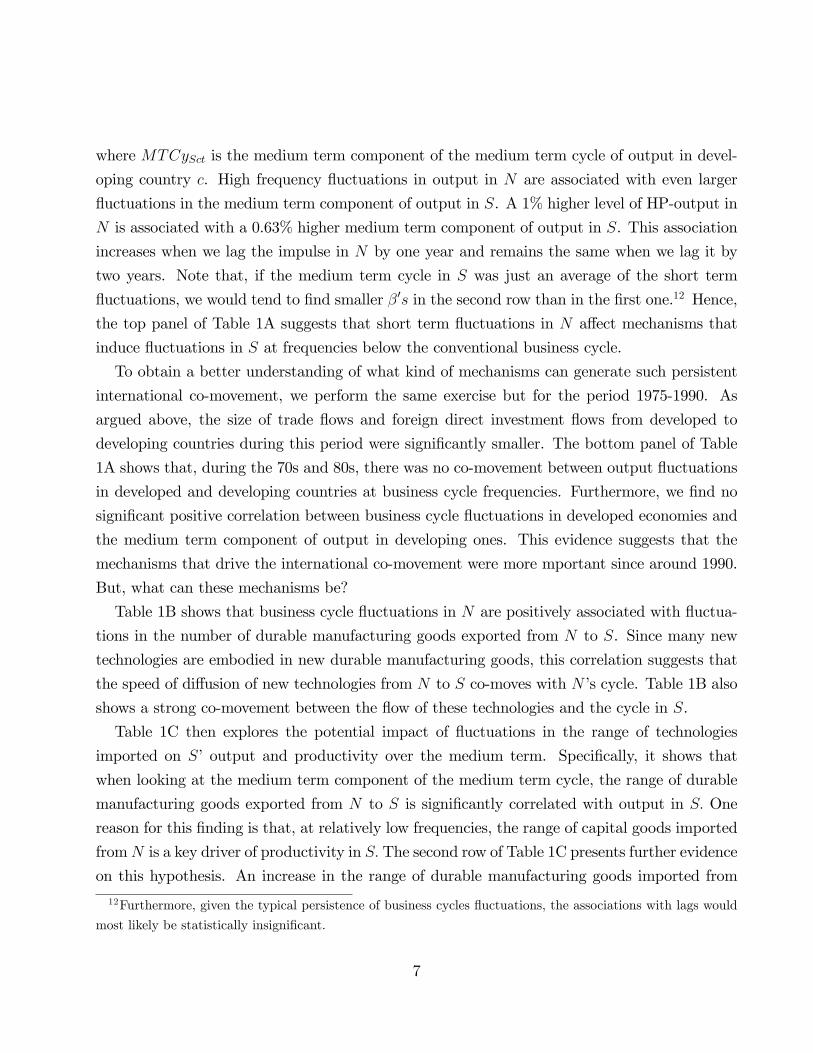
where MTCySct is the medium term component of the medium term cycle of output in devel-

oping country c. High frequency fluctuations in output in N are associated with even larger

fluctuations in the medium term component of output in S. A 1% higher level of HP-output in

N is associated with a 0.63% higher medium term component of output in S. This association

increases when we lag the impulse in N by one year and remains the same when we lag it by

two years. Note that, if the medium term cycle in S was just an average of the short term

fluctuations, we would tend to find smaller β′s in the second row than in the first one.12 Hence,

the top panel of Table 1A suggests that short term fluctuations in N affect mechanisms that

induce fluctuations in S at frequencies below the conventional business cycle.

To obtain a better understanding of what kind of mechanisms can generate such persistent

international co-movement, we perform the same exercise but for the period 1975-1990. As

argued above, the size of trade flows and foreign direct investment flows from developed to

developing countries during this period were significantly smaller. The bottom panel of Table

1A shows that, during the 70s and 80s, there was no co-movement between output fluctuations

in developed and developing countries at business cycle frequencies. Furthermore, we find no

significant positive correlation between business cycle fluctuations in developed economies and

the medium term component of output in developing ones. This evidence suggests that the

mechanisms that drive the international co-movement were more mportant since around 1990.

But, what can these mechanisms be?

Table 1B shows that business cycle fluctuations in N are positively associated with fluctua-

tions in the number of durable manufacturing goods exported from N to S. Since many new

technologies are embodied in new durable manufacturing goods, this correlation suggests that

the speed of diffusion of new technologies from N to S co-moves with N’s cycle. Table 1B also

shows a strong co-movement between the flow of these technologies and the cycle in S.

Table 1C then explores the potential impact of fluctuations in the range of technologies

imported on S’output and productivity over the medium term. Specifically, it shows that

when looking at the medium term component of the medium term cycle, the range of durable

manufacturing goods exported from N to S is significantly correlated with output in S. One

reason for this finding is that, at relatively low frequencies, the range of capital goods imported

fromN is a key driver of productivity in S. The second row of Table 1C presents further evidence

on this hypothesis. An increase in the range of durable manufacturing goods imported from

12Furthermore, given the typical persistence of business cycles fluctuations, the associations with lags would

most likely be statistically insignificant.

7

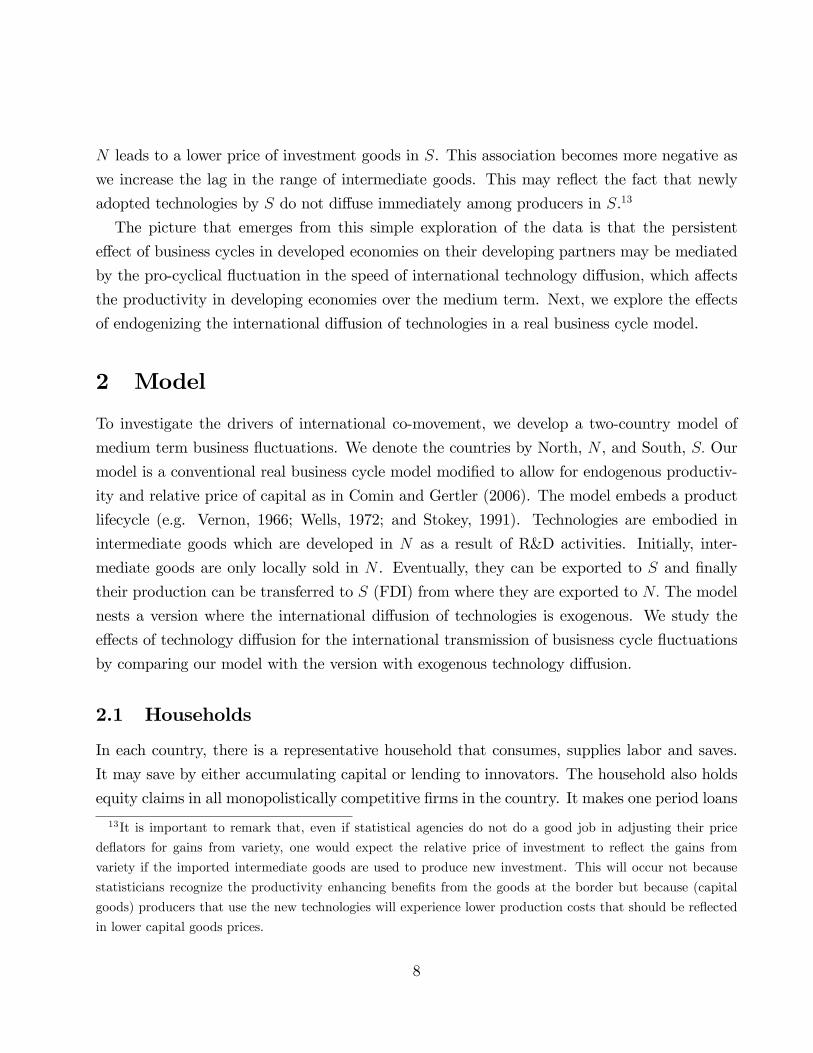
N leads to a lower price of investment goods in S. This association becomes more negative as

we increase the lag in the range of intermediate goods. This may reflect the fact that newly

adopted technologies by S do not diffuse immediately among producers in S.13

The picture that emerges from this simple exploration of the data is that the persistent

effect of business cycles in developed economies on their developing partners may be mediated

by the pro-cyclical fluctuation in the speed of international technology diffusion, which affects

the productivity in developing economies over the medium term. Next, we explore the effects

of endogenizing the international diffusion of technologies in a real business cycle model.

2 Model

To investigate the drivers of international co-movement, we develop a two-country model of

medium term business fluctuations. We denote the countries by North, N , and South, S. Our

model is a conventional real business cycle model modified to allow for endogenous productiv-

ity and relative price of capital as in Comin and Gertler (2006). The model embeds a product

lifecycle (e.g. Vernon, 1966; Wells, 1972; and Stokey, 1991). Technologies are embodied in

intermediate goods which are developed in N as a result of R&D activities. Initially, inter-

mediate goods are only locally sold in N . Eventually, they can be exported to S and finally

their production can be transferred to S (FDI) from where they are exported to N. The model

nests a version where the international diffusion of technologies is exogenous. We study the

effects of technology diffusion for the international transmission of busisness cycle fluctuations

by comparing our model with the version with exogenous technology diffusion.

2.1 Households

In each country, there is a representative household that consumes, supplies labor and saves.

It may save by either accumulating capital or lending to innovators. The household also holds

equity claims in all monopolistically competitive firms in the country. It makes one period loans

13It is important to remark that, even if statistical agencies do not do a good job in adjusting their price

deflators for gains from variety, one would expect the relative price of investment to reflect the gains from

variety if the imported intermediate goods are used to produce new investment. This will occur not because

statisticians recognize the productivity enhancing benefits from the goods at the border but because (capital

goods) producers that use the new technologies will experience lower production costs that should be reflected

in lower capital goods prices.

8

to innovators and rents capital to firms. Physical capital does not flow across countries. There

is no international lending and borrowing and the only international capital flow is N ′s FDI in

S.

Let Cct be consumption and µwct a shock to the disutility of working. Then the household

maximizes its present discounted utility as given by the following expression:

Et∞∑i=0

βt+i

[lnCct − µwct

(Lct)ζ+1

ζ + 1

], (1)

subject to the budget constraint

Cct = ωctLct + Πct +DctKct − P kctJct +RctBct −Bct+1 (2)

where Πct reflects corporate profits paid out fully as dividends to households, Dct denotes the

rental rate of capital, Jct is investment in new capital, P kct is the price of investment, and Bct

is the total loans the household makes at t − 1 that are payable at t. Rct is the (possibly

state-contingent) payoff on the loans.

The household’s stock of capital evolves as follows:

Kct+1 = (1− δ(Uct))Kct + Jct, (3)

where δ(Uct) is the depreciation rate which is increasing and convex in the utilization rate as

in Greenwood, Hercowitz and Huffman (1988).

The household’s decision problem is simply to choose consumption, labor supply, capital and

bonds to maximize equation (1) subject to (2) and (3).

2.2 Technology

The sophistication of the production process in country c depends on the number of intermediate

goods available for production, Act. There are three types of intermediate goods. There are

Alt local intermediate goods that are only available for production in N . There are Agt global

intermediate goods that have successfully diffused to S. These goods are produced in N and

exported to S, and are available for production in both N and S. There are ATt intermediate

goods whose production has been transferred to S. These goods are exported from S to N and

are available for production in both N and S. The total number of intermediate goods in each

9

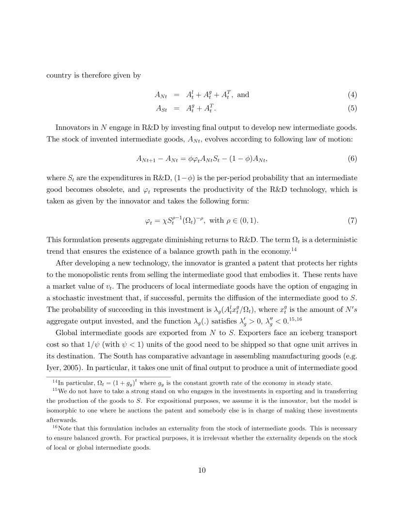
country is therefore given by

ANt = Alt + Agt + ATt , and (4)

ASt = Agt + ATt . (5)

Innovators in N engage in R&D by investing final output to develop new intermediate goods.

The stock of invented intermediate goods, ANt, evolves according to following law of motion:

ANt+1 − ANt = φϕtANtSt − (1− φ)ANt, (6)

where St are the expenditures in R&D, (1−φ) is the per-period probability that an intermediate

good becomes obsolete, and ϕt represents the productivity of the R&D technology, which is

taken as given by the innovator and takes the following form:

ϕt = χSρ−1t (Ωt)−ρ, with ρ ∈ (0, 1). (7)

This formulation presents aggregate diminishing returns to R&D. The term Ωt is a deterministic

trend that ensures the existence of a balance growth path in the economy.14

After developing a new technology, the innovator is granted a patent that protects her rights

to the monopolistic rents from selling the intermediate good that embodies it. These rents have

a market value of vt. The producers of local intermediate goods have the option of engaging in

a stochastic investment that, if successful, permits the diffusion of the intermediate good to S.

The probability of succeeding in this investment is λg(Altxgt/Ωt), where x

gt is the amount of N

′s

aggregate output invested, and the function λg(.) satisfies λ′g > 0, λ′′g < 0.15 ,16

Global intermediate goods are exported from N to S. Exporters face an iceberg transport

cost so that 1/ψ (with ψ < 1) units of the good need to be shipped so that ogne unit arrives in

its destination. The South has comparative advantage in assembling manufacturing goods (e.g.

Iyer, 2005). In particular, it takes one unit of final output to produce a unit of intermediate good

14In particular, Ωt = (1 + gy)t where gy is the constant growth rate of the economy in steady state.

15We do not have to take a strong stand on who engages in the investments in exporting and in transferring

the production of the goods to S. For expositional purposes, we assume it is the innovator, but the model is

isomorphic to one where he auctions the patent and somebody else is in charge of making these investments

afterwards.16Note that this formulation includes an externality from the stock of intermediate goods. This is necessary

to ensure balanced growth. For practical purposes, it is irrelevant whether the externality depends on the stock

of local or global intermediate goods.

10

in N , while if the intermediate good is assembled in S, it only takes 1/ξ(< 1) units of country

S output. Producers of global intermediate goods may take advantage of this cost advantage

by transferring the production of the global intermediate goods to S. As for exporting, we

model the transfer of production a stochastic investment. The probability of succeding in this

investment is λT (AgtxTt /Ωt), where the function λT (.) satisfies λ′T > 0, λ′′T < 0, and xTt is the

amount of S ′s aggregate output invested. We denote by et the relative price of N ′s output in

terms of S (i.e., the exchange rate). Because xT is S ′s aggregate output invested by a foreign

firm to start producing in S, we denote it as FDI.

Given this product cycle structure, the stock of global and transferred intermediate goods

evolve according to the following laws of motion:

Agt+1 = φλg(Altxgt/Ωt)A

lt + φ(1− λT (Agtx

Tt /Ωt))A

gt (8)

ATt+1 = φλT (AgtxTt /Ωt)A

gt + φATt . (9)

2.3 Production

The production side of the economy is composed of two sectors that produce, respectively,

aggregate output and investment. In both sectors, we allow for entry and exit that amplifies

business cycle shocks in a way similar to price or wage rigidities. In addition it allows our

model to capture the high-frequency counter-cyclicality of the relative price of investment which

is an important feature of business cycles. The dynamics of intermediate goods described in

the previous subsection determine the stock of intermediate goods available for production in

each country. Intermediate goods are embodied in new investment goods and determine their

effi ciency over the medium and long term. For simplicity, disembodied technological change is

taken as exogenous.17

Aggregate output is produced competitively by combining the outputs produced by Nyct

differentiated producers as follows:

Yct =

[∫ Nyct

0

[Yjct]1/µ dj

]µ(10)

Each differentiated producer has access to the following production function:

Yjct = χct (UcjtKcjt)α (Lcjt)

1−α , (11)

17Comin and Gertler (2006) endogenize both embodied and disembodied technological change in a one country

setting.

11

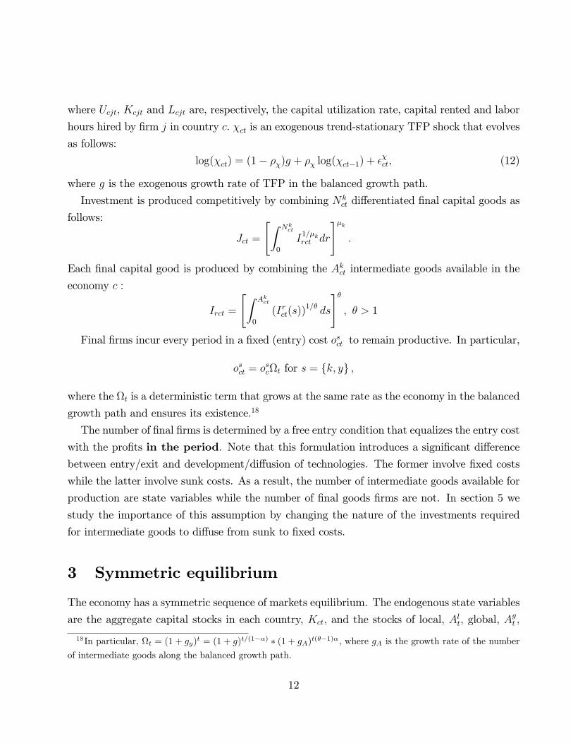
where Ucjt, Kcjt and Lcjt are, respectively, the capital utilization rate, capital rented and labor

hours hired by firm j in country c. χct is an exogenous trend-stationary TFP shock that evolves

as follows:

log(χct) = (1− ρχ)g + ρχ log(χct−1) + εχct, (12)

where g is the exogenous growth rate of TFP in the balanced growth path.

Investment is produced competitively by combining Nkct differentiated final capital goods as

follows:

Jct =

[∫ Nkct

0

I1/µkrct dr

]µk.

Each final capital good is produced by combining the Akct intermediate goods available in the

economy c :

Irct =

[∫ Akct

0

(Irct(s))1/θ ds

]θ, θ > 1

Final firms incur every period in a fixed (entry) cost osct to remain productive. In particular,

osct = oscΩt for s = k, y ,

where the Ωt is a deterministic term that grows at the same rate as the economy in the balanced

growth path and ensures its existence.18

The number of final firms is determined by a free entry condition that equalizes the entry cost

with the profits in the period. Note that this formulation introduces a significant differencebetween entry/exit and development/diffusion of technologies. The former involve fixed costs

while the latter involve sunk costs. As a result, the number of intermediate goods available for

production are state variables while the number of final goods firms are not. In section 5 we

study the importance of this assumption by changing the nature of the investments required

for intermediate goods to diffuse from sunk to fixed costs.

3 Symmetric equilibrium

The economy has a symmetric sequence of markets equilibrium. The endogenous state variables

are the aggregate capital stocks in each country, Kct, and the stocks of local, Alt, global, Agt ,

18In particular, Ωt = (1 + gy)t = (1 + g)t/(1−α) ∗ (1 + gA)t(θ−1)α, where gA is the growth rate of the number

of intermediate goods along the balanced growth path.

12

and transferred, ATt , intermediate goods. The following system of equations characterizes the

equilibrium.

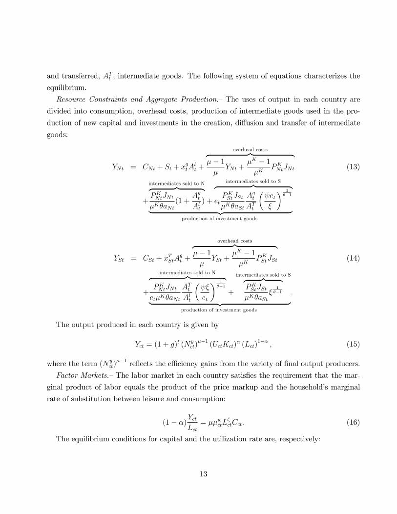
Resource Constraints and Aggregate Production.—The uses of output in each country are

divided into consumption, overhead costs, production of intermediate goods used in the pro-

duction of new capital and investments in the creation, diffusion and transfer of intermediate

goods:

YNt = CNt + St + xgtAlt +

overhead costs︷ ︸︸ ︷µ− 1

µYNt +

µK − 1

µKPKNtJNt (13)

+

intermediates sold to N︷ ︸︸ ︷PKNtJNt

µKθaNt(1 +

AgtAlt

) +

intermediates sold to S︷ ︸︸ ︷etPKStJSt

µKθaSt

AgtATt

(ψetξ

) 1θ−1

︸ ︷︷ ︸production of investment goods

YSt = CSt + xTStAgt +

overhead costs︷ ︸︸ ︷µ− 1

µYSt +

µK − 1

µKPKStJSt (14)

+

intermediates sold to N︷ ︸︸ ︷PKNtJNt

etµKθaNt

ATtAlt

(ψξ

et

) 1θ−1

+

intermediates sold to S︷ ︸︸ ︷PKStJSt

µKθaStξ

1θ−1︸ ︷︷ ︸

production of investment goods

.

The output produced in each country is given by

Yct = (1 + g)t (Nyct)

µ−1 (UctKct)α (Lct)

1−α , (15)

where the term (Nyct)

µ−1 reflects the effi ciency gains from the variety of final output producers.

Factor Markets.—The labor market in each country satisfies the requirement that the mar-

ginal product of labor equals the product of the price markup and the household’s marginal

rate of substitution between leisure and consumption:

(1− α)YctLct

= µµwctLζctCct. (16)

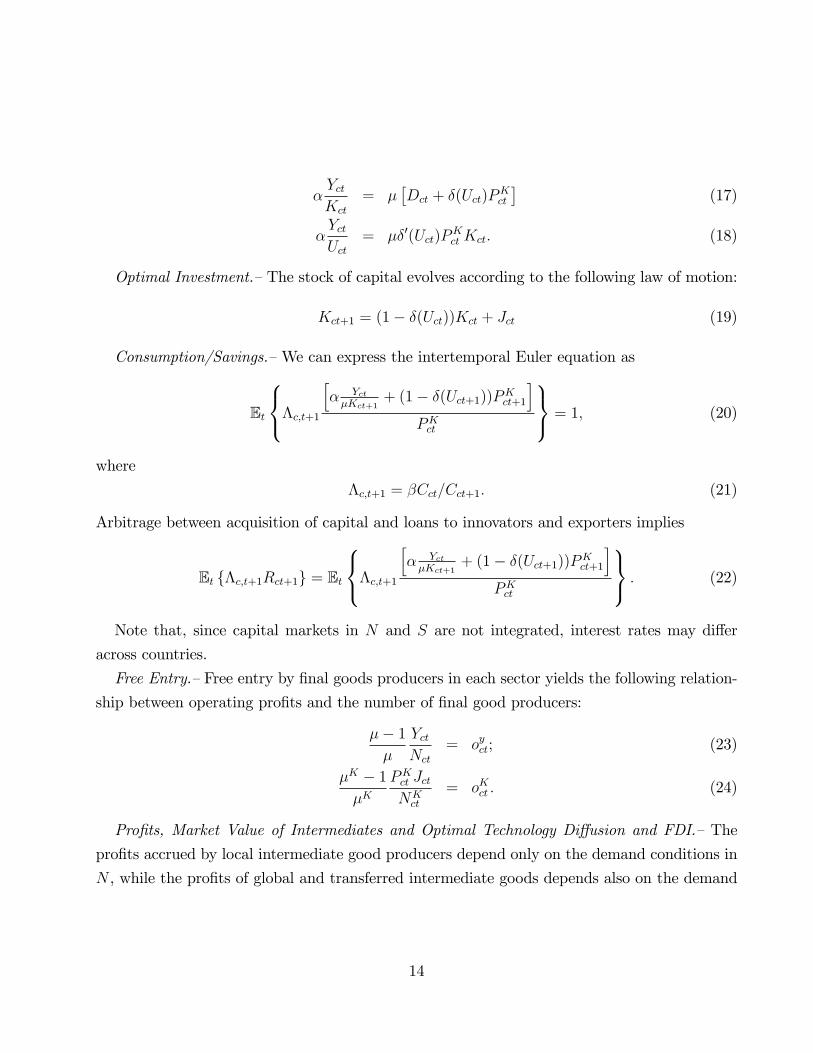
The equilibrium conditions for capital and the utilization rate are, respectively:

13

αYctKct

= µ[Dct + δ(Uct)P

Kct

](17)

αYctUct

= µδ′(Uct)PKct Kct. (18)

Optimal Investment.—The stock of capital evolves according to the following law of motion:

Kct+1 = (1− δ(Uct))Kct + Jct (19)

Consumption/Savings.—We can express the intertemporal Euler equation as

Et

Λc,t+1

[α YctµKct+1

+ (1− δ(Uct+1))PKct+1

]PKct

= 1, (20)

where

Λc,t+1 = βCct/Cct+1. (21)

Arbitrage between acquisition of capital and loans to innovators and exporters implies

Et Λc,t+1Rct+1 = Et

Λc,t+1

[α YctµKct+1

+ (1− δ(Uct+1))PKct+1

]PKct

. (22)

Note that, since capital markets in N and S are not integrated, interest rates may differ

across countries.

Free Entry.—Free entry by final goods producers in each sector yields the following relation-

ship between operating profits and the number of final good producers:

µ− 1

µ

YctNct

= oyct; (23)

µK − 1

µKPKct JctNKct

= oKct . (24)

Profits, Market Value of Intermediates and Optimal Technology Diffusion and FDI.—The

profits accrued by local intermediate good producers depend only on the demand conditions in

N , while the profits of global and transferred intermediate goods depends also on the demand

14

in S. Specifically, they are given by

πt =

(1− 1

θ

)PKNtJNt

µkaNtAlt

(25)

πgt =

(1− 1

θ

)PKNtJNt

µkaNtAlt

+

(1− 1

θ

)etPKStJSt

µkaStATt

(ψetξ

) 1θ−1

, (26)

πTt =

(1− 1

θ

)PKNtJNt

µkaNtAlt

(ψξ

et

) 1θ−1

+

(1− 1

θ

)etPKStJSt

µkaStATt

, (27)

where aNt is the ratio of the effective number of intermediate goods in N relative to Alt, and

aSt is the ratio of the effective number of intermediate goods in S relative to ATt :

aNt =

[1 +

AgtAlt

+ATtAlt

(ψξ

et

) 1θ−1]

; (28)

aSt =

[AgtATt

(ψetξ

) 1θ−1

+ 1

]. (29)

The market value of companies that currently hold the patent of a local, global and trans-

ferred intermediate good are, respectively,

vt = πt − xgt + φEt

ΛN,t+1

[λg(A

ltxgt/Ωt)v

gt+1 +

(1− λT (Agtx

Tt /Ωt)

)vt+1

], (30)

vgt = πgt − etxTt + (31)

φEt

ΛN,t+1

[λT (Agtx

Tt /Ωt)v

Tt+1 +

(1− λT (Agtx

Tt /Ωt)

)vgt+1

],

vTt = πTt + φEt

ΛN,t+1vTt+1

, (32)

where the optimal investments in exporting and transferring the production of intermediate

goods from N to S are given by the optimality conditions

1 = φ(Alt/Ωt

)λ′g(A

ltxgt/Ωt)Et

ΛN,t+1

(vgt+1 − vt+1

), (33)

et = φ (Agt/Ωt)λ′T (Agtx

Tt /Ωt)Et

ΛN,t+1

(vTt+1 − v

gt+1

). (34)

The optimal investment, xg and xT , equalize, at the margin, the cost and expected benefit

of exporting the intermediate good to S and of transferring the production of the intermediate

good to S.19 The marginal cost of investing one unit of output in exporting the good is 1,

19Given the symmetry between these two FOCs, we discuss only the exporting decision.

15

while the expected marginal benefit is equal to the increase in the probability of international

diffusion times the discounted gain frommaking the intermediate good global(i.e., vgt+1 − vt+1

).

Equation (31) illustrates why the international diffusion of technologies is procyclical. The value

of global intermediate goods is approximately equal to the value of local goods plus the value

from exporting goods to S. Since demand in S is pro-cyclical, the capital gain from exporting

an intermediate good (i.e. vgt+1 − vt+1) is pro-cyclical. It follows then from (33) that, since λg

is a concave function, xgt is pro-cyclical.

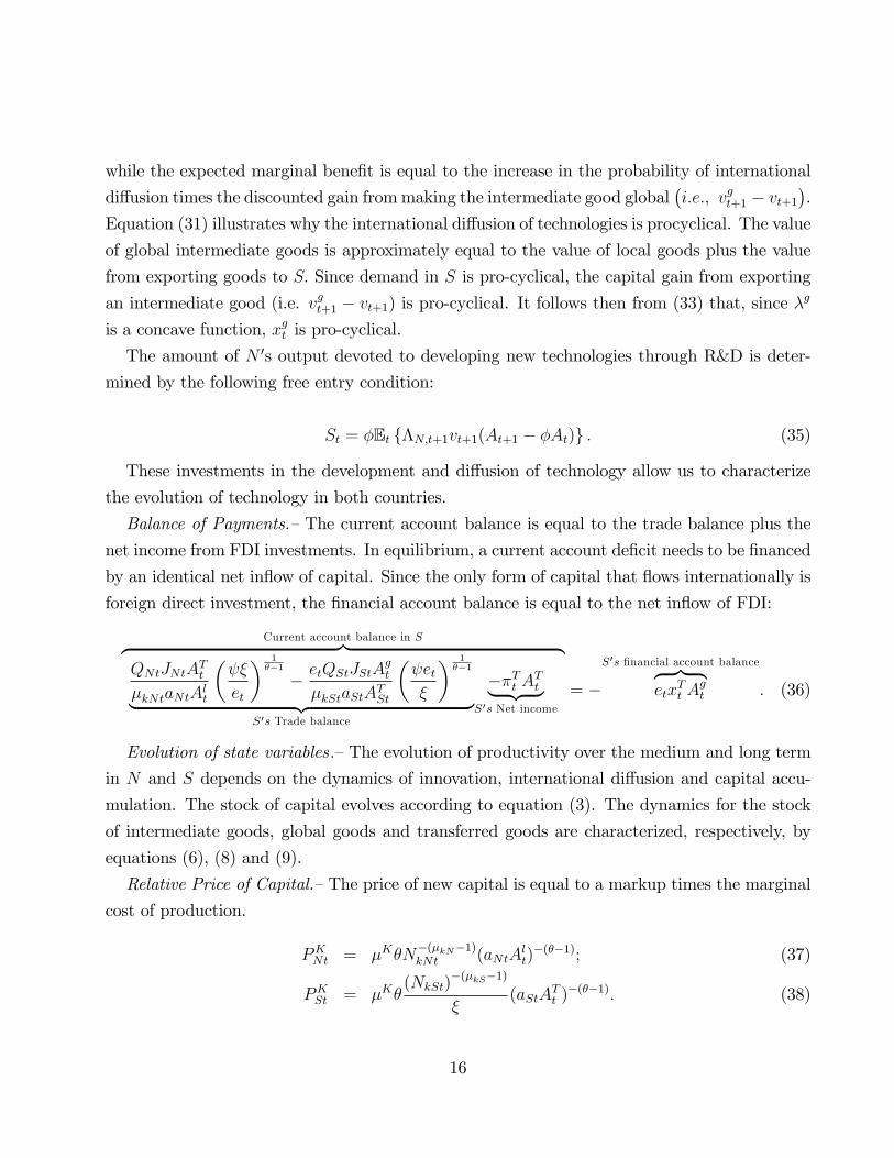
The amount of N ′s output devoted to developing new technologies through R&D is deter-

mined by the following free entry condition:

St = φEt ΛN,t+1vt+1(At+1 − φAt) . (35)

These investments in the development and diffusion of technology allow us to characterize

the evolution of technology in both countries.

Balance of Payments.—The current account balance is equal to the trade balance plus the

net income from FDI investments. In equilibrium, a current account deficit needs to be financed

by an identical net inflow of capital. Since the only form of capital that flows internationally is

foreign direct investment, the financial account balance is equal to the net inflow of FDI:

Current account balance in S︷ ︸︸ ︷QNtJNtA

Tt

µkNtaNtAlt

(ψξ

et

) 1θ−1

− etQStJStAgt

µkStaStATSt

(ψetξ

) 1θ−1

︸ ︷︷ ︸S′s Trade balance

−πTt ATt︸ ︷︷ ︸S′s Net income

= −S′s financial account balance︷ ︸︸ ︷

etxTt A

gt . (36)

Evolution of state variables.—The evolution of productivity over the medium and long term

in N and S depends on the dynamics of innovation, international diffusion and capital accu-

mulation. The stock of capital evolves according to equation (3). The dynamics for the stock

of intermediate goods, global goods and transferred goods are characterized, respectively, by

equations (6), (8) and (9).

Relative Price of Capital.—The price of new capital is equal to a markup times the marginal

cost of production.

PKNt = µKθN

−(µkN−1)kNt (aNtA

lt)−(θ−1); (37)

PKSt = µKθ

(NkSt)−(µkS−1)

ξ(aStA

Tt )−(θ−1). (38)

16

Observe from (37) and (38) that the effi ciency gains associated with Act and Nkct reduce the

marginal cost of producing investment. Fluctuations in these variables are responsible for the

evolution in the short, medium and long run of the price of new capital, PKct . However, Act and

Nkct affect P

Kct at different frequencies.

Because Act is a state variable, it does not fluctuate in the short term. Increases in Act reflect

embodied technological change and drive the long-run trend in the relative price of capital.

Pro-cyclical investments in the development and diffusion of new intermediate goods lead to

pro-cyclical fluctuations in the growth rate of Act, generating counter-cyclical movements in PKct

over the medium term. Nkct, instead, is a stationary jump variable. Therefore, the entry/exit

dynamics drive only the short term fluctuations in PKct .

Exogenous technology diffusion .—The version of the model with exogenous technology dif-

fusion we study below is characterized by the same system of equations with the exeption that

xg and xT are fixed at their steady state levels. That is, at the levels in which equations (33)

and (34) hold along the balanced growth path.

4 Model Evaluation

In this section we explore the ability of the model to generate cycles at short and medium term

frequencies that resemble those observed in the data in developed and, especially, in developing

economies. Given our interest in medium term fluctuations, a period in the model is set to

a year. We solve the model by log-linearizing around the deterministic balanced growth path

and then employing the Anderson-Moore code, which provides numerical solutions for general

first order systems of difference equations.20 We describe the calibration before turning to some

numerical exercises.

4.1 Calibration

The calibration we present here is meant as a benchmark. We have found that our results are

robust to reasonable variations around this benchmark. To the greatest extent possible, we

use the restrictions of balanced growth to pin down parameter values. Otherwise, we look for

evidence elsewhere in the literature. There are a total of twenty-three parameters summarized

in Table 2. Eleven appear routinely in other studies. Six relate to the process of innovation

20Anderson and Moore (1983).

17

and R&D and were used, among others, in Comin and Gertler (2006). Finally, there are six

new parameters that relate to trade and the process of international diffusion of intermediate

goods. We defer the discussion of the calibration of the standard and R&D parameters to

the Appendix and focus here on the adjustment costs parameters and those that govern the

interactions between N and S.

We calibrate the six parameters that govern the interactions between N and S by matching

information on trade flows, and U.S. FDI in Mexico, the micro evidence on the cost of exporting

and the relative productivity of U.S. and Mexico in manufacturing. First, we set ξ to 2 to match

Mexico’s relative cost advantage over the U.S. in manufacturing identified by Iyer (2005). We

set the inverse of the iceberg transport cost parameter, ψ, to 0.95,21 the steady state probability

of exporting an intermediate good, λg, to 0.0875, and the steady state probability of transferring

the production of an intermediate good to S, λT , to 0.0055. This approximately matches the

share of Mexican exports and imports to and from the U.S. in Mexico’s GDP (i.e. 18% and 14%,

respectively) and the share of intermediate goods produced in the U.S. that are exported to

Mexico. Specifically, Bernard, Jensen, Redding and Schott (2007) estimate that approximately

20 percent of U.S. durable manufacturing plants export. However, these plants produce a

much larger share of products than non-exporters. As a result, the share of intermediate

goods exported should also be significantly larger. We target a value of 33% for the share of

intermediate goods produced in the U.S. that are exported. This yields an average diffusion

lag to Mexico of 11 years, which seems reasonable given the evidence (e.g. Comin and Hobijn,

2010).

Das, Roberts and Tybout (2007) have estimated that the sunk cost of exporting for Colom-

bian manufacturing plants represents between 20 and 40 percent of their annual revenues from

exporting. We set the elasticity of λg with respect to investments in exporting, ρg, to 0.8 so that

the sunk cost of exporting represents approximately 30 percent of the revenues from exporting.

The elasticity of λT with respect to FDI expenses, ρT , together with the steady state value of

λT , determine the share of U.S. FDI in Mexico in steady state. We set ρT to 0.5 so that U.S.

FDI in Mexico represents approximately 2% of Mexican GDP.

21Interestingly, the value of ψ required to match the trade flows between the US and Mexico is smaller than

the values used in the literature (e.g. 1/1.2 in Corsetti et al., 2008) because of the closeness of Mexico and the

US and their lower (nonexistent after 1994) trade barriers.

18

4.2 Impulse response functions

In our model there are several variables that can be the sources of economic fluctuations. For

concreteness, we present most of our results using TFP shocks (i.e. shocks to the level of

disembodied productivity) both in the U.S. and Mexico as the source of fluctuations. However,

as we show below, our findings are robust to alternative sources of fluctuations such as shocks

to the price of investment and to the wedge markup. Throughout, we use solid lines for the

responses in Mexico and dashed lines for the responses in the U.S.

Exogenous international diffusion.—We start by considering the version of our economy

where the rate of international diffusion of technologies is fixed (Figure 2). That is, λT and λg

are constant and equal to their steady state values (i.e., 0.0875 and 0.0055, respectively). The

response of the U.S. economy to a domestic TFP shock is very similar to the single-country

version presented in Comin and Gertler (2006). In particular, a negative TFP shock reduces

the marginal product of labor and capital causing a drop in hours worked (panel 2) and in

the utilization rate of capital. The drop in hours worked and in the utilization rate causes a

recession (panel 1). The response of U.S. output to the shock is more persistent than the shock

itself (panel 12) due to the endogenous propagation mechanisms of the model. In particular,

the domestic recession reduces the firms’incentives to invest in physical capital and that leads

to a drop in teh demand for intermediate goods. As a result, the return to R&D investments

also drops, leading to a temporary decline in the rate of development of new technologies but

to a permanent effect on the level of new technologies relative to trend. The long-run effect of

the shock on output is approximately forty percent of its initial response.

The U.S. shock has important effects on Mexico’s economy in the short term. When the

U.S. experiences a recession, the demand for Mexican intermediate goods declines (i.e. intensive

margin of trade). In addition, the lower current and future output reduces Mexican investment

upon impact. The decline in aggregate demand is matched by an equivalent drop in Mexican

aggregate supply caused by a reduction in the utilization rate of capital, hours worked and net

entry (which leads to a reduction in the effi ciency of final output production). However, unlike

the estimates from Tables 1A-1C, the response of the Mexican economy to the U.S. shock is

monotonic, less persistent, and always smaller than the response of the U.S. economy. This

is also the case for the wage markup and price of investment shocks (see Figure A1 in the

non-published Appendix).

Correlated shocks.—A brute-force way to increase the impact of U.S. shocks in Mexico is

19

to impose an exogenous correlation in the shocks processes of the U.S. and Mexican economy.

This fix raises the question of what could be driving the correlation of the shocks. In reality,

few shocks are international in nature. Therefore, the cross-country correlation between shocks

should be relatively small. Indeed, if we focus on TFP shocks, the empirical contemporaneous

cross-country correlation in TFP tends to be relatively small. For the case of Mexico and the

US, the correlation between HP-filtered annual TFP since 1990 is 0.39.22

Despite these caveats, it may still be instructive to explore how allowing for cross-country

correlation in TFP shocks affects the response of the Mexican economy to a U.S. shock. Figure

3 plots the impulse response to a U.S. shock when calibrating the contemporaneous effect of

U.S. TFP on Mexico TFP at 0.4, which we regard as an upper bound.23 Despite the exogenous

correlation of the shocks, we continue to find that both the impact of the U.S. shock and,

especially, the peristence of its effects are larger in the U.S. than in Mexico. We therefore

conclude that the model with exogenous technology diffusion does not capture the pattern of

international co-movemnet we have documented in section 2.

Endogenous international technology diffusion.—Next, we explore the role of the endogenous

diffusion of technologies in the international propagation of shocks. Figure 4 plots the response

to a contractionary shock to U.S. TFP in the full-blown model. The response of the U.S.

economy is very similar to Figure 2, where international diffusion was exogenous. This is the

case because potential feed-backs from Mexico are negligible for the U.S. Also, as in Figure 2,

the U.S. shock has an important effect on the Mexican economy, upon impact. The magnitude

of the initial response is similar because the initial propagation channel is the same (a drop

in the demand for Mexican exports). However, the shape and persistence of the response

changes significantly once we allow for the speed of intenational technology diffusion to vary

endogenously. In particular, the response of the Mexican economy to a U.S. shock is hump-

shaped; within two years, it surpases the effect that the shock has on the U.S. itself, reaching

the maximum impact approximately within five years. After ten years, the effect of the shock

in Mexican output is still similar to the initial impact.

Why such a protracted and non-monotonic impact of U.S. shocks in Mexico? By endogenizing

the diffusion of technology from the U.S. to Mexico, we introduce new margins of pro-cyclical

22Since 1980 it is -0.02 and since 1950 it is 0.11.23Kehoe and Perri (2002) set the cross-country correlation of TFP shocks in their two-country model to 0.25

which they claim is in line with the VAR estimates of U.S. and a subsample of Western European countries

(Baxter and Crucini, (1995), Kollmann (1996) and Backus, Kehoe and Kydland (1992)).

20

variation in the state variables that govern the medium term dynamics of productivity in

Mexico, Ag and AT . More specifically, contractionary shocks such as a negative shock to U.S.

TFP reduce the return to exporting new intermediate goods and to transferring their production

to Mexico. As a result, fewer resources are devoted to these investments, xg and xT , (panel

7). Because the stock of Mexican technologies (Ag and AT ) are state variables, declines in

xg and xT only generate a gradual reduction of the stock of intermediate goods available for

production in Mexico relative to the steady state (panel 8). Since the stock of intermediate

goods determines the productivity in the capital producing sector, this results in a reduction in

the productivity of capital which manifests itself in a higher relative price of investment (panel

6) over the medium term.

The prospect of lower aggregate demand, initially, reduces investment causing net exit of

final investment good producers. Due to the presence of effi ciency gains from the number of

final capital producers, exit reduces the effi ciency in the production of investment goods causing

an initial increase in the price of investment (panel 6).24 However, note that the initial drop

of investment in Mexico is smaller than in the U.S. This is the case because, in Mexico, the

price of investment is expected to increase more than in the U.S. Since investment is cheap

relative to its future price, Mexican firms, initially, undertake smaller cuts in investment. As

the price of invetsment gradually increases, Mexican investment drops further contributing

to the subsequent drop in output. This is how the endogenous diffusion and international

transfer of technologies generate a hump-shaped response for the number of intermediate goods,

productivity, investment and output in Mexico.25

One may wonder about the nature and values of the parameters that affect the hump-shaped

response of Mexican technology to the U.S. shock. Inspection of the laws of motion of Ag and AT

(equations 8 and 9) suggests that the elasticities of diffusion and technology transfer with respect

to xg and xT are key in governing these dynamics. In particular, they play two roles. First, for

given investments xg and xT , the elasticities determine the contribution of the investments to

the number of intermediate goods available for production (and produced) in Mexico. Second,

from the optimal investment equations (33) and (34), the higher the elasticities, the larger are

24The price of investment also increases upon impact due to the shift in the use from foreign to domestically-

produced intermediate goods after the initial depreciation of the peso (to be discussed below).25The effect that the international diffusion of technology has on the persistence of output in developing

countries can provide a microfoundation for the finding of Aguiar and Gopinath (2007) that (in a reduced

form specification) the shocks faced by developing countries are more persistent than those faced by developed

economies.

21

the fluctuations in xg and xT in response to a given expected capital gain. These intuitions

are illustrated in Figure 5 where we plot the impulse response function to a U.S. TFP shock

in a version of the model where we have calibrated the elasticities of λg and λT with respect

to xg and xT to 0.2 (instead of our baseline values of 0.8 and 0.5, respectively). We consider

that this calibration captures a key aspect of the pre-NAFTA/pre-globalization period where

investments in FDI and in exporting new goods were much less prominent. As Figure 5 shows,

in this scenario, U.S. shocks had a much more transitory effect on Mexican macro variables.26

Still, one may wonder why is it the case that medium termfluctuations in Mexican technology

in response to a U.S. shock may be larger than in the U.S. itself. This is the result of various

forces. First, the stock of technologies available for production is smaller in Mexico than in

the U.S.; therefore, a given change in the flow of new technologies will tend to generate larger

fluctuations over the medium term in the stock of available technologies. Second, anticipating

the effects that a given fluctuation in xg and xT have on Ag and AT (and therefore on output and

investment), over the medium term, xg and xT tend to drop more than R&D, S, in response to

a contractionary U.S. shock. The final element that contributes to generating a higher eventual

impact of the U.S. shock in Mexico than in the U.S. itself is the exchange rate (panel 11,

where an increase represents a real appreciation in Mexico vis a vis the U.S.). The depreciation

of the peso in response to the shock has opposite effects in the effective stock of available

intermediate goods in the U.S. and Mexico. In the U.S., a depreciation of the peso makes

transferred intermediate goods more attractive increasing the effective number of intermediate

goods available for production (i.e., aNt ∗ Alt); in Mexico, instead, the depreciation of the pesomakes more expensive imported intermediate goods reducing the effi ency gains from using

global intermediate goods and hence the effective number of available intermediate goods (i.e.,

aSt ∗ Agt ).We conclude our qualitative exploration of the model’s response to a U.S. shock by studying

the impact on the exchange rate. In steady state, there is a net inflow of FDI to Mexico in

the form of the investments made by multinationals that want to transfer the production of

intermediate goods to Mexico. The surplus in the financial account implies that in steady state,

Mexico has a deficit in the current account. Since, its trade balance with the U.S. is positive,

in our model, the negative current account balance comes from the negative net income due

to the repatriation of multinational profits. Following a contractionary U.S. shock, the decline

26In results not reported, we have shown that the initial impact of the U.S. shock in Mexico also is smaller

when we calibrate higher transport costs so that the volume of trade is smaller.

22

in the return to transferring production to Mexico, causes a large drop in FDI inflows (i.e.,

xT , panel 7), a phenomenon that echoes the “sudden stops”literature (e.g. Calvo, 1998). The

drop in FDI inflows reduces the ability of the Mexican economy to finance its current account

deficit. Despite the reduction in net income outflows (due to the reduction in multinational

profits, πT ), restoring the balance of payments requires the peso to depreciate, and in this way

reduce the volume of U.S. exports to Mexico. Hence, the depreciation of the peso that follows

a contractionary U.S. shock.

Response to a Mexican Shock.—To complete our analysis of the model’s impulse responses,

we study the effects of Mexican TFP shocks (see Figure 6). There are some striking differences

with the response to the U.S. shock. First, a Mexican shock has a very small effect in the U.S.

This follows from the difference in size between the two economies. One consequence is that

the Mexican shock has a much smaller effect on U.S. R&D investments than the U.S. shock. As

a result, the slowdown in the flow of intermediate goods to Mexico is less protracted than for

the U.S. shock (panel 8) generating a less persistent response of Mexican output. This in turn

leads to more muted firms’responses in their investment decisions. In particular, the Mexican

shock leads to smaller reductions by U.S. firms in the resources they invest in exporting and

transfering the production of intermediate goods to Mexico (panel 7). Similarly, Mexican firms

respond by cutting domestic investment in physical capital by less (panel 4). As a result, of

these differences, the fluctuations in the range of technologies available for production in Mexico

is smaller and less protracted in response to the Mexican shock than to the US shock.

In addition to the dynamics of technology, another element that dampens the effect of the

shock on the Mexican economy is the exchange rate (panel 11). Unlike the U.S. shock, a

contractionary TFP shock to Mexico leads to an appreciation of the peso. The response of the

real exchange rate affects the behavior of the investment-output ratio in both countries. In

Mexico, the investment-output ratio drops less than with the U.S. shock because now Mexican

firms can import U.S. intermediate goods more cheaply. In the U.S., the appreciation of the

peso makes imported intermediate goods more expensive reducing the effective productivity

of the investment sector (panel 6). Firms respond to the higher investment prices by cutting

invetsment a lot (relative to the actual drop in U.S. output) (panel 4). This same logic accounts

for the worsening of the Mexican trade balance.

Finally, the last feature of the impulse response functions that deserve attention is the

response of domestic interest rates to a Mexican shock. As shown by Neumeyer and Perri

(2005), an important feature of business cycles in developing countries is the counter-cyclicality

23

of real interest rates. Our model delivers this result endogenously (panel 5). In our model,

the procyclical diffusion of technologies generates counter-cyclical fluctuations in the relative

price of capital. This is the case because, as one can see from expression (22), interest rates in

our model not only reflect the marginal product of capital but also the capital gains from the

appreciation in the price of capital. The pro-cyclical diffusion of technologies induces counter-

cyclical capital gains from holding a unit of capital. In the case of the domestic Mexican shock,

this second effect dominates the pro-cyclical response of the marginal product of capital (i.e.

the dividend), thus inducing interest rates in S (as well as the interest differential with respect

to N) to be counter-cyclical.

4.3 Simulations

We next turn to the quantitative evaluation of the model. To this end, we calibrate the volatility

and persistence of TFP shocks in the U.S. and Mexico and run 1000 simulations over a 17-year

long horizon each. Since we intend to evaluate the model’s ability to propagate shocks both

internationally and over time, we use the same autocorrelation for both U.S. andMexican shocks

and set the cross-country correlation of the shocks to zero. We set the annual autocorrelation

of TFP shocks to 0.8 to match the persistence of output in the U.S.27

We calibrate the volatility of the shocks by forcing the model to approximately match the

high frequency standard deviation of GDP in Mexico and the U.S. This yields a volatility of the

TFP shocks of 2.16% in the U.S. and 3.73% in Mexico. This is consistent with the suspicion

that developing economies are prone to bigger disturbances than developed countries.

Volatility.—Table 3 compares the standard deviations of the high frequency and mediumterm cycle fluctuations in the data and in the model. Our calibration strategy forces the model

to match the volatilities of output in Mexico and the U.S. at the high frequency. In addition,

the model also comes very close to matching the volatility of output over the medium term

both in Mexico (0.045 vs. 0.037 in the data) and in the U.S. (0.022 vs. 0.015 in the data).

Given the low persistence of shocks, matching these moments suggests that the model induces

the right amount of propagation of high frequency shocks into the medium term.

The model does a good job in reproducing the volatility observed in the data in most variables

27See Comin and Gertler (2006) for details. Note that, because of the propagation obtained from the endoge-

nous technology mechanisms, this class of models requires a smaller autocorrelation of the shocks to match the

persistence in macro variables. In short, they are not affected by the Cogley and Nason (1995) criticism that

the Neoclassical growth model does not propagate exogenous disturbances.

24

other than output. The model generates series for investment, bilateral trade flows, and FDI

flows that have similar volatilities to those observed in the data both at the high frequency and

medium term. For those instances where there are some differences, the empirical volatilities

tend to fall within the 95% confidence interval for the standard deviation of the simulated series.

The model tends to underpredict teh volatility of the relative price of capital, and the extensive

margin of trade. This however, is an indication that our calibration of the endogenous diffusion

mechanisms does not overstate its importance relative to the data. The variable where the

model fails is consumption. The model underpredicts the volatility of consumption in Mexico,

especially at the high frequency. This may be a reflection of our model’s lack of financial

frictions in developing countries which may enhance the volatility of consumption in the data.

In the U.S., instead, consumption is about as volatile in the model as in the data.

Co-movement.—Most international business cycle models have problems reproducing the

cross-country co-movement patterns observed in macro variables. First, they lack international

propagation mechanisms that induce a strong positive co-movement in output. Second, they

tend to generate a stronger cross-country co-movement in consumption than in output, while

in the data we observe the opposite (Backus, Kehoe and Kydland, 1992).28

Our model fares well in both of these dimensions. Panel A of Table 4 reports the cross

country correlations between Mexico and the U.S. for consumption and output, both in the

model and in the data. The model generates the strong co-movement between U.S. and Mexico

GDPs observed in the data. The average cross-country correlation in our simulations is 0.72

with a confidence interval of (0.4 , 0.9) that contains the correlation observed in the data (0.43).

The model also generates a smaller cross-country correlation for consumption than for output,

as we observe in the data: The average cross-correlation is 0.31 with a confidence interval that

contains the empirical correlation (0.2).29

The endogenous diffusion of technology contributes to generating this cross-country co-

movement pattern. Intuitively, the endogenous diffusion of technology generates a strong

cross-country co-movement in output and productivity over the medium term. Anticipating

28Several authors, including Baxter and Crucini (1995) and Kollmann (1996), have shown that reducing the

completeness of international financial markets is not suffi cient to match the data along these dimensions. Kehoe

and Perri (2002) have made significant progress by introducing enforcement contraints on financial contracts.

This mechanism limits the amount of risk sharing, reducing consumption co-movement and increasing the

cross-country co-movement in output. However, output still co-moves significantly less than in the data.29The international business cycle literature has also found it diffi cult to generate positive cross-correlations

in investment and employment (Baxter, 1995). As it is clear from Figure 4, our model delivers both.

25

the future evolution of the economy, Mexican firms adjust investment contemporaneously. The

large effect that foreign shocks have on domestic investment limits the possibility for a large

consumption response, hence inducing a higher cross-country correlation in output than in

consumption.

Panel B of Table 4 reports the contemporaneous correlation between the HP-filtered Mexican

variables and HP-filtered output in both Mexico and the U.S.30 Broadly speaking, the model

does a good job in capturing the contemporaneous co-movement patterns within Mexico but

also between Mexico and the U.S. The model generates a positive, albeit insignificant correlation

between consumption and output in Mexico (0.47 vs. 0.78 in the data). Also, in both model

and data, Mexico’s consumption is more correlated with Mexico’s GDP than with the U.S.

The model captures the strong co-movement between Mexican investment and output in both

the U.S. (0.78 vs. 0.6 in the data) and Mexico (0.99 vs. 0.62 in the data). In our model, the

pro-cyclical response of investment is in part due to the counter-cyclicality of the relative price

of investment. Our model approximately matches the co-movement between Mexico’s output

and the price of new capital (-0.8 vs. -0.54 in the data), although it overstates the co-movement

between the price of capital in Mexico and U.S. GDP (-0.9 in model vs. 0.13 in data). Similarly,

recall that the medium term productivity dynamics in Mexico result from the cyclicality of the

flow of intermediate goods that diffuse to Mexico (i.e. the extensive margin of trade). The

model matches quite closely the correlation between our data-counterpart for this variable and

output in both the U.S. (0.42 vs. 0.28 in the data) and in Mexico (0.36 vs. 0.42 in the data).

The model also captures broadly the cyclicality of the bilateral trade flows. In particular,

the model generates the strong counter-cyclicality of Mexico’s trade balance. The correlation

between Mexico’s trade balance and GDP is -0.96 vs. -0.83 in the data. This is the case because,

both in the data and in our model, imports from the U.S. co-move more with Mexico’s GDP

than exports to the U.S. However, the model overpredicts the cycality of Mexican exports to the

U.S. (with respect to Mexican GDP). The model approximately captures the high correlation

of bilateral trade flows with U.S. GDP.

A variable where the model underperforms is FDI. Though the model matches the cyclicality

of FDI in the data, the correlations with both U.S. and Mexico’s GDP are too high. This may

reflect the presence of a small but volatile component in actual FDI that does not respond to

the U.S. or Mexican business cycle. This hypothesis seems to be supported by the fact that

30Note that we do not filter the growth rate of intermediate goods since this variable is already trend stationary.

26

FDI is much more persistent in our model than in the data.31

Inter-frequency Co-movement.—One of the motivations for our model was the observation

that U.S. high frequency fluctuations lead medium term fluctuations in Mexico. The impulse

response functions to U.S. shocks (see Figure 2) show that, qualitatively, the model is able

to generate these persistent effects. Table 5 explores the quantitative power of the model to

reproduce the inter-frequency co-movement patterns we observe in the data. The first row

of Table 5 reports the empirical correlation between lagged HP-filtered U.S. output and the

medium term component of Mexico’s output. The second row reports the average of these

statistics across 1000 simulations of the model.

The model roughly captures the contemporaneous correlation between high frequency fluc-

tuations in U.S. output and medium term fluctuations in Mexico’s output (0.33 in the model

vs. 0.28 in the data). More importantly, the model generates a hump-shaped cross-correlogram

between these two variables as we observed in the data. However, in the data the peak cor-

relation occurs after two years (0.53), while in the model it occurs on average after one year

(0.37).

A key prediction of our model is that the high frequency response of FDI and the extensive

margin of trade to U.S. shocks generates counter-cyclical fluctuations in the relative price of

capital in Mexico over the medium term. The fourth row in Table 5 presents the average cor-

relation across our 1000 simulations between the medium term component of Mexico’s relative

price of capital and HP-filtered U.S. output at various lags. In both actual and simulated data,

the contemporaneous correlation is insignificant. The correlation becomes more negative as we

lag U.S. GDP in both cases. In the simulated data the peak (in absolute terms) is reached after

one years (-0.44), while in the actual data it is reached after three years (-0.5).

Unlike U.S. shocks, Mexican shocks do not have a hump-shaped effect on Mexico’s output

over the medium term fluctuations. The correlation between HP-filtered and the medium term

component of Mexico’s output is positive and declines monotonically as we lag the series of

HP-filtered output.32 Our model is consistent with this co-movement pattern. (See rows 5 and

6 in Table 5.)33

31In particular, the annual autocorrelation of FDI/GDP in our model is 0.42 while in the data it is -0.35.32In the working paper version, we make a similar point by estimating VARs with HP-filtered Mexico’s GDP

and the medium term component of several Mexican variables (including GDP).33A similar (but negative) co-movement patter is generated in the model between Hp-filtered output and teh

medium term component of teh relative price of capital in Mexico. In the data the co-movementbetween these

variables is also negative but insignificant. (See rows 7 and 8 in Table 5.)

27

5 Discussion

Next, we explore in more detail the implications of our model and compare it to existing models

of trade and international business cycles.

Other Shocks.—For concreteness, we have used TFP shocks as the sole source of fluctuations

in our simulations. However, our findings are not driven by the nature of the shocks. To

illustrate this, we introduce shocks to the wage markup and to the price of investment. Figure

7 presents the impulse response functions to a (positive) wage markup shock (second row) and

a (positive) shock to the price of investment (third row) both in the U.S. To facilitate the

comparison, the impulse response function to the U.S. TFP shock is presented in the first row

of the figure.

Qualitatively, the impulse response functions to these shocks are very similar. In all of them

there is a large effect upon the impact of the U.S. shock on Mexican output. All shocks generate

a hump-shaped response of Mexico’s output. And in all three cases, the U.S. shock eventually

has a larger effect on Mexico than in the U.S. The economics of the response are the same as

in the TFP shock described above. All three shocks trigger a large and persistent slowdown in

the flow of new technologies to Mexico and an initial decline in Mexico’s investment larger than

the initial decline in consumption. As the productivity of the capital goods sector deteriorates

relative to trend, investment declines further generating the hump in the output response. The

response to Mexican shocks is also robust to the nature of the shocks (see Figure A2).

Sunk vs. Fixed Exporting Costs.—Much of the theoretical international macro literature that

has incorporated the extensive margin of trade has relied on extensions of the Melitz (2003)

model. The Melitz model is a two country model with firms of heterogenous productivity and

where firms have to incur in some costs to export. Unlike our model, most of the models that

have used the Melitz framework to explore business cycle dynamics use fixed cost instead of

sunk cost to adjust the range of intermediate goods available for production.

The empirical literature on firm dynamics and exports has found that there are large sunk

costs of exporting new products (e.g. Roberts and Tybout, 1997; Das et al., 2007). However,

the use of fixed costs could be defended on the grounds of their tractability if the model with

fixed costs has propagation and amplification power similar to that of the model with sunk costs

of exporting. To explore whether this is the case, we develop a version of our model where,

to export intermediate goods, firms in N now just need to incur a per period fixed cost. For

consistency, we also make the investment in transferring production from N to S a fixed cost.

28

Other than these two changes, this version of the model is identical to our original model. This

model is basically a variation on the financial autarky model in Ghironi and Melitz (2005) with

physical capital and without heterogeneity. We calibrate the fixed costs of exporting and FDI

so that in steady state the trade flows are the same as in our original model.

Figure 8 plots the impulse response functions to a (negative) TFP shock in the U.S. in

the model with fixed costs. The differences with our original model are remarkable. In the

model with fixed costs of exporting and FDI, a contractionary U.S. shock causes no effect in

Mexico’s output upon impact. The sharp contrast between the responses in figures 4 and 7 is

ultimately due to the different nature of the costs of technology diffusion in the two models.

With the fixed costs of exporting and transferring technologies, the stock of technologies in S

depends on the profits accrued by local, global and transferred intermediate goods and on the

exchange rate. Since all these are jump variables, this means that Ag and AT are no longer

state variables. As a result, investments in exporting and transferring production no longer have

persistent effects on the productivity level in S. As a result, productivity in S fluctuates less

over the medium term, generating also a more muted response of the relative price of capital.

Anticipating smaller increases in the price of investment and smaller drops in future demand,

Mexican firms undertake smaller cuts in their investment, upon impact. The smaller response

of investment in Mexico has two significant feedback effects. First, it leads to a smaller drop in

the profits accrued by intermediate goods producers in Mexico, further dampening the response

of investments in technology diffusion. Second, the smaller drop in Mexican investment implies

that now Mexican net exports are counter-cyclical, while with the sunk cost formulation they

responded pro-cyclically to U.S. shocks. As a result, in response to a contractionary shock to

U.S. TFP, net exports increase dampening further the impact on Mexican output of the shock.

Implications for Aggregate Volatility.—It is clear from Figure 4 that U.S. shocks are a signif-

icant source of volatility in Mexico’s GDP. But what share of Mexican fluctuations is due to

U.S. shocks and what share is due to domestic shocks? Similarly, how much do Mexican shocks

contribute to the volatility of U.S. GDP?

Table 6 answers these questions by reporting the share of output volatility in each country

attributable to each kind of shock. The first two columns focus on the volatility of HP-filtered

output while the next two focus on the volatility of output over the medium term cycle. Con-

sistent with Figure 6, Mexican shocks account for a small fraction of U.S. fluctuations (10% at

high frequency and 11% over the medium term cycle).

In contrast, U.S. shocks represent a very significant source of Mexican fluctuations. At

29

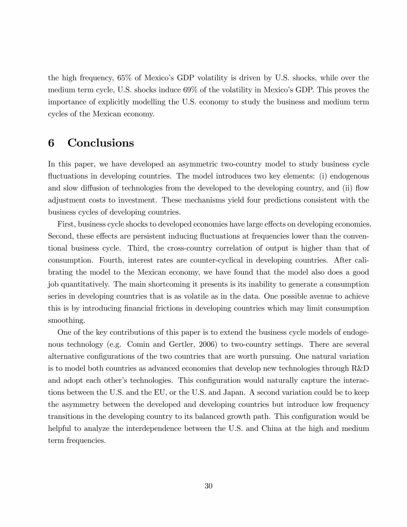
the high frequency, 65% of Mexico’s GDP volatility is driven by U.S. shocks, while over the

medium term cycle, U.S. shocks induce 69% of the volatility in Mexico’s GDP. This proves the

importance of explicitly modelling the U.S. economy to study the business and medium term

cycles of the Mexican economy.

6 Conclusions

In this paper, we have developed an asymmetric two-country model to study business cycle

fluctuations in developing countries. The model introduces two key elements: (i) endogenous

and slow diffusion of technologies from the developed to the developing country, and (ii) flow

adjustment costs to investment. These mechanisms yield four predictions consistent with the

business cycles of developing countries.

First, business cycle shocks to developed economies have large effects on developing economies.

Second, these effects are persistent inducing fluctuations at frequencies lower than the conven-

tional business cycle. Third, the cross-country correlation of output is higher than that of

consumption. Fourth, interest rates are counter-cyclical in developing countries. After cali-

brating the model to the Mexican economy, we have found that the model also does a good

job quantitatively. The main shortcoming it presents is its inability to generate a consumption

series in developing countries that is as volatile as in the data. One possible avenue to achieve

this is by introducing financial frictions in developing countries which may limit consumption

smoothing.

One of the key contributions of this paper is to extend the business cycle models of endoge-

nous technology (e.g. Comin and Gertler, 2006) to two-country settings. There are several

alternative configurations of the two countries that are worth pursuing. One natural variation

is to model both countries as advanced economies that develop new technologies through R&D

and adopt each other’s technologies. This configuration would naturally capture the interac-

tions between the U.S. and the EU, or the U.S. and Japan. A second variation could be to keep

the asymmetry between the developed and developing countries but introduce low frequency

transitions in the developing country to its balanced growth path. This configuration would be

helpful to analyze the interdependence between the U.S. and China at the high and medium

term frequencies.

30

References

[1] Aguiar, M. and G. Gopinath (2007). “Emerging Market Business cycle: The Trend is The

Cycle”Journal of Political Economy. Vol. 115: 69-102.

[2] Anderson, G., and G. Moore (1983). “An Effi cient Procedure for Solving Linear Perfect

Foresight Models.”Board of Governors of the Federal Reserve System mimeo.

[3] Backus, D., F. Kydland, and P. Kehoe (1992). “International Real Business Cycles,” Jour-

nal of Political Economy Vol. 100, No. 4: 745-775.

[4] Basu, S., and J. Fernald (1997). “Returns to Scale in U.S. Production: Estimates and

Implications,”Journal of Political Economy Vol. 105, No. 2: 249-283.

[5] Baxter, M. (1995). “International Trade and Business Cycles”Handbook of International

Economics, G. Grossman and K. Rogoff (eds.), Vol. 3 (Amsterdam: Noth-Holland), p.

1901-1864.

[6] Baxter, M. and M. Crucini (1995). “Business Cycles and the Asset Structure of Foreign

Trade,”International Economic Review, Vol. 36, No. 4., pp. 821-854.

[7] Bergin, P., R. Feenstra, G. Hanson (2009). “Volatility Due to Offshoring: Theory and

Evidence”mimeo U.C. Davis.

[8] Bernard, A., B. Jensen, S. Redding and P. Schott (2007). “Firms and International Trade”

mimeo.

[9] Broda, C. and D. Weinstein (2006). “Globalization and the Gains from Variety,”Quarterly

Journal of Economics, Vol. 121, Issue 2 - May 2006

[10] Burnstein, A., C. Kurz, and L. Tesar (2008): “Trade, Production Sharing and the Inter-

national Transmission of Business Cycles”Journal of Monetary Economics, Vol. 55, No.

4: 775-795.

[11] Caballero, R., and A. Jaffe (1993). “How High are the Giants’Shoulders: An Empirical

Assessment of Knowledge Spillovers and Creative Destruction in a Model of Economic

Growth,”NBER Macroeconomics Annual, O. J. Blanchard and S. Fischer editors, MIT

press, p. 15-72.

31

[12] Calvo, G. (1998). “Capital Flows and Capital-Market Crises: The Simple Economics of

Sudden Stops,”Journal of Applied Economics Vol. 1, No. 1: 35-54.

[13] Comin, D. (2007). “On the Integration of Growth and Business Cycles,”Empirica, Vol.

36, No. 2(May).

[14] Comin, D. and M. Gertler (2006). “Medium-Term Business Cycles,”American Economic

Review Vol. 96, No. 3: 523-551.

[15] Comin, D., M. Gertler and A. M. Santancreu (2008), “Innovations in Growth Potential as

Sources of Output and Asset Price Fluctuations" mimeo.

[16] Das, S., M. Roberts and J. Tybout (2007). “Market entry Costs, Producer Heterogeneity

and Export Dynamics”Econometrica, Vol. 75, No. 3 (May): 837-873.

[17] Gali, J., M. Gertler and D. Lopez-Salido (2007), “Markups, Gaps, and the Welfare Cost of

Economic Fluctuations”, Review of Economics and Statistics, Vol. 89 (February):. 44-59.

[18] Ghironi, F., and M. Melitz (2005). “International Trade and Macroeconomic Dynamics

with Heterogeneous Firms”Quarterly Journal of Economics, Vol. 120, No. 3: 865-915.

[19] Greenwood, J., Z. Hercowitz and G. W. Huffman (1988). “Investment, Capacity Utiliza-

tion, and the Real Business Cycle,”The American Economic Review Vol. 78, No. 3: 402-

417.

[20] Greenwood, J., Z. Hercowitz, and P. Krusell (1997), "Long-Run Implications of Investment-

Specific Technological Change," American Economic Review Vol. 87, n. 3: 342-362.

[21] Greenwood, J., Z. Hercowitz and P. Krusell (2000). “The role of investment-specific tech-

nological change in the business cycle,”European Economic Review Vol. 44, No. 1: 91-115.

[22] Greenwood, J. and M. Yorukoglu (1997), "1974," Carnegie-Rochester Conference Series

on Public Policy, Vol. 46: 49-95.

[23] Iyer, L. (2003). “NAFTA: To Trade or not To Trade,”HBS case #9-705-034.

[24] Griliches, Z. (1990). “Patent Statistics as Economic Indicators: A Survey.” Journal of

Economic Literature, 28(4), pp. 1661—707.

32

[25] Kehoe, P. and F. Perri (2002). “International Business CyclesWith Endogenous Incomplete

Markets,”Econometrica. Vol. 70, No. 3: 907-928, May.

[26] Kollman, R. (1996). “Incomplete Asset Markets and the Cross-Country Consumption Cor-

relation Puzzle,”Journal of Economic Dynamics and Control, Vol.20, pp.945-962.

[27] Loayza, N. and L. Serven (2006). “Capital flows to Developing Countries: The Old and

The New”mimeo.

[28] Mendoza, E. (2008). “Sudden Stops, Financial Crises and Leverage: A Fisherian Deflation

of Tobin’s Q”The American Economic Review (forthcoming).

[29] Neumeyer, P. and F. Perri (2005). “Business Cycles in Emerging Economies: The Role of

Interest Rates," Journal of Monetary Economics Vol. 52, No. 2: pp. 345-380.

[30] Pakes, A. and M. Schankerman (1984). “The Rate of Obsolescence of Knowledge, Research

gestation Lags, and the Private Rate of Return to Research Resources” p. 73-88, in Z.

Griliches (Ed.), Patents, R&D and Productivity, The University of Chicago Press.

[31] Romer, Paul M.(1990). “Endogenous Technological Change,”Journal of Political Economy

Vol. 98, No.5: 71-102

[32] Stokey, Nancy (1991). “The Volume and Composition of Trade between Rich and Poor

Countries”Review of Economic Studies Vol. 58, No. 1: 63-80, January.

[33] Vernon, Raymond (1966). “International Investment and International Trade in the Prod-

uct Cycle,”The Quarterly Journal of Economics Vol.80, No. 2: 190-207.

[34] Zlate, A. (2010): “Offshore Production and Business Cycle Dynamics with Heterogeneous

Firms,”International Finance Discussion Paper 2010-995, Board of Governors of the Fed-

eral Reserve System

33

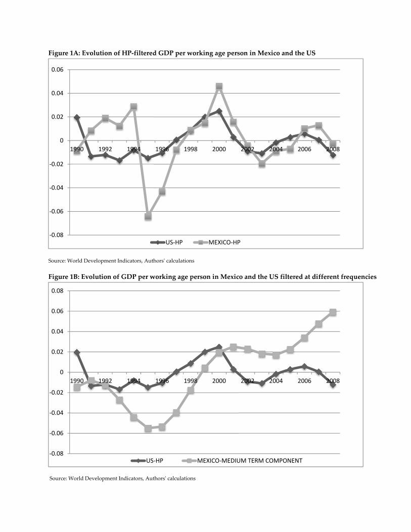
Figure 1A: Evolution of HP‐filtered GDP per working age person in Mexico and the US

Source: World Development Indicators, Authorsʹ calculations

Figure 1B: Evolution of GDP per working age person in Mexico and the US filtered at different frequencies

Source: World Development Indicators, Authorsʹ calculations

‐0.08

‐0.06

‐0.04

‐0.02

0

0.02

0.04

0.06

1990 1992 1994 1996 1998 2000 2002 2004 2006 2008

US‐HP MEXICO‐HP

‐0.08

‐0.06

‐0.04

‐0.02

0

0.02

0.04

0.06

0.08

1990 1992 1994 1996 1998 2000 2002 2004 2006 2008

US‐HP MEXICO‐MEDIUM TERM COMPONENT

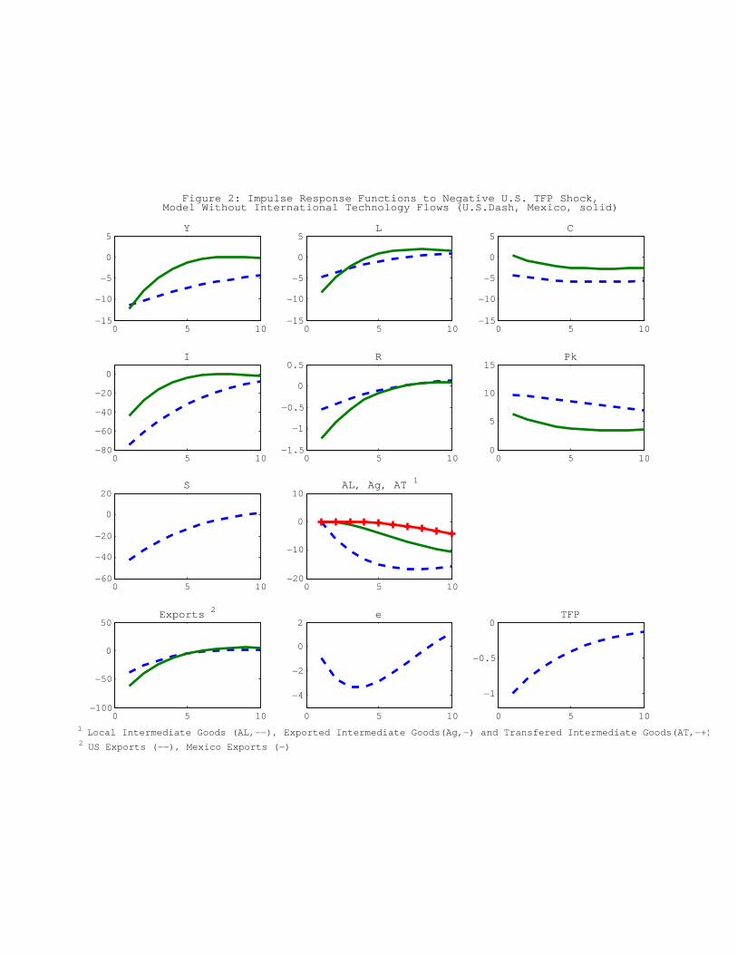
0 5 10−15

−10

−5

0

5Y

0 5 10−15

−10

−5

0

5L

0 5 10−15

−10

−5

0

5C

0 5 10−80

−60

−40

−20

0

I

0 5 10−1.5

−1

−0.5

0

0.5R

0 5 100

5

10

15Pk

0 5 10−60

−40

−20

0

20S

0 5 10−20

−10

0

10AL, Ag, AT 1

1 Local Intermediate Goods (AL,−−), Exported Intermediate Goods(Ag,−) and Transfered Intermediate Goods(AT,−+)

0 5 10−100

−50

0

50Exports 2

2 US Exports (−−), Mexico Exports (−)

0 5 10

−4

−2

0

2e

0 5 10

−1

−0.5

0TFP

Figure 2: Impulse Response Functions to Negative U.S. TFP Shock,Model Without International Technology Flows (U.S.Dash, Mexico, solid)

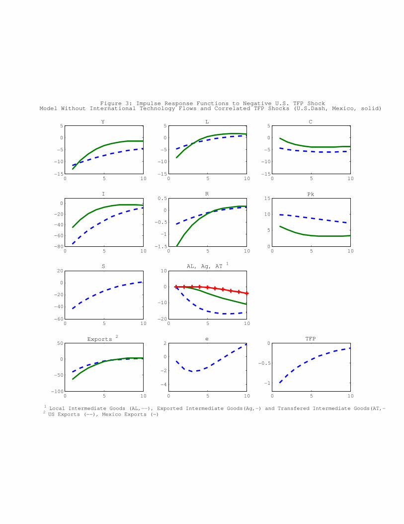
0 5 10−15

−10

−5

0

5Y

0 5 10−15

−10

−5

0

5L

0 5 10−15

−10

−5

0

5C

0 5 10−80

−60

−40

−20

0

I

0 5 10−1.5

−1

−0.5

0

0.5R

0 5 100

5

10

15Pk

0 5 10−60

−40

−20

0

20S

0 5 10−20

−10

0

10AL, Ag, AT 1

1 Local Intermediate Goods (AL,−−), Exported Intermediate Goods(Ag,−) and Transfered Intermediate Goods(AT,−+)

0 5 10−100

−50

0

50Exports 2

2 US Exports (−−), Mexico Exports (−)

0 5 10

−4

−2

0

2e

0 5 10

−1

−0.5

0TFP

Figure 3: Impulse Response Functions to Negative U.S. TFP ShockModel Without International Technology Flows and Correlated TFP Shocks (U.S.Dash, Mexico, solid)

0 5 10−15

−10

−5

0

5Y

0 5 10−15

−10

−5

0

5L

0 5 10−15

−10

−5

0

5 C

0 5 10−80

−60

−40

−20

0

I

0 5 10−1.5

−1

−0.5

0

0.5R

0 5 100

2

4

6

8

10Pk

0 5 10−80

−60

−40

−20

0

20S Xg, Xt 1

1 Research and development expenditures (S, −−), investments in exporting (Xg,−) and FDI (Xt, −+)

0 5 10−20

−15

−10

−5

0

5

10AL, Ag, AT 2

2 Local Intermediate Goods (AL,−−), Exported Intermediate Goods(Ag,−) and Transfered Intermediate Goods(AT,−+)

0 5 10−60

−40

−20

0

20ΠT and VT 3

3 Net income from transferred intermediate goods (−−), Value of transferred intermediate goods (−)

0 5 10−100

−50

0

50Exports 4

4 US Exports (−−), Mexico Exports (−)

0 5 10−5

0

5e

0 5 10

−1

−0.8

−0.6

−0.4

−0.2

0TFP

Figure 4: Impulse Response Functions to Negative U.S. TFP Shock, Endogenous Technology Diffusion (U.S.Dash, Mexico, solid)

0 5 10−15

−10

−5

0

5Y

0 5 10−15

−10

−5

0

5L

0 5 10−15

−10

−5

0

5C

0 5 10−80

−60

−40

−20

0

I

0 5 10−1.5

−1

−0.5

0

0.5R

0 5 100

5

10Pk

0 5 10−80

−60

−40

−20

0

20S Xg, Xt 1

1 Research and development expenditures (S, −−), investments in exporting (Xg,−) and FDI (Xt, −+)

0 5 10−20

−10

0

10AL, Ag, AT 2

2 Local Intermediate Goods (AL,−−), Exported Intermediate Goods(Ag,−) and Transfered Intermediate Goods(AT,−+)

0 5 10−80

−60

−40

−20

0

20ΠT and VT 3

3 Net income from transferred intermediate goods (−−), Value of transferred intermediate goods (−)

0 5 10−100

−50

0

50Exports 4

4 US Exports (−−), Mexico Exports (−)

0 5 10−5

0

5e

0 5 10

−1

−0.5

0TFP

Figure 5: Impulse Response Functions to Negative U.S. TFP Shock Pre−NAFTA, Endogenous Technology Diffusion(U.S.Dash, Mexico, solid)

0 5 10−6

−4

−2

0

2Y

0 5 10−6

−4

−2

0

2L

0 5 10−6

−4

−2

0

2C

0 5 10−20

−15

−10

−5

0

5

10I

0 5 10−0.5

0

0.5R

0 5 10−1

−0.5

0

0.5

1Pk

0 5 10−20

−10

0

10

20S Xg, Xt 1

1 Research and development expenditures (S, −−), investments in exporting (Xg,−) and FDI (Xt, −+)

0 5 10−5

0

5AL, Ag, AT 2

2 Local Intermediate Goods (AL,−−), Exported Intermediate Goods(Ag,−) and Transfered Intermediate Goods(AT,−+)

0 5 10−20

−10

0

10

20ΠT and VT 3

3 Net income from transferred intermediate goods (−−), Value of transferred intermediate goods (−)

0 5 10−20

−10

0

10

20Exports 4

4 US Exports (−−), Mexico Exports (−)

0 5 10−3

−2

−1

0

1

2

3e

0 5 10

−1

−0.8

−0.6

−0.4

−0.2

0TFP

Figure 6: Impulse Response Functions to Negative Mexico TFP Shock, Endogenous Technology Diffusion (U.S.Dash, Mexico, solid)

0 5 10−15

−10

−5

0Y

0 5 10−15

−10

−5

0C

0 5 10−60

−50

−40

−30

−20

−10

0I

0 5 10−60

−50

−40

−30

−20

−10

0

10

20S Xg, Xt 1

0 5 10−5

−4

−3

−2

−1

0Y

0 5 10−5

−4

−3

−2

−1

0C

0 5 10−20

−15

−10

−5

0I

0 5 10−40

−30

−20

−10

0

10

20S Xg, Xt 1

1 Research and development expenditures (S, −−), investments in exporting (Xg,−) and FDI (Xt, −+)

0 5 10−10

−8

−6

−4

−2

0

Y

0 5 10−10

−8

−6

−4

−2

0

C

0 5 10−40

−35

−30

−25

−20

−15

−10

−5

0I

0 5 10−40

−30

−20

−10

0

10

20S Xg, Xt 1

Figure 7: Impulse Response Functions for U.S. TFP, Wage Markup and Price of Investment Shocks, Baseline Model (U.S. Dash, Mexico, solid)

TFP(negative)

Markup

Price ofInvestment

0 5 10−10

−5

0

5Y

0 5 10−10

−5

0

5L

0 5 10−10

−5

0

5C

0 5 10−60

−40

−20

0

I

0 5 10−0.5

0

0.5R

0 5 100

1

2

3

4

5Pk

0 5 10−40

−20

0

20S

0 5 10−20

0

20

40AL, Ag, AT 1

1 Local Intermediate Goods (AL,−−), Exported Intermediate Goods(Ag,−) and Transfered Intermediate Goods(AT,−+)

0 5 10−40

−30

−20

−10

0

10Exports 2

2 US Exports (−−), Mexico Exports (−)

0 5 10

−2

0

2

e

0 5 10

−1

−0.5

0TFP

Figure 8: Impulse Response Functions to Negative U.S. TFP Shock, Model with Fixed Costs of International Technology Diffusion (U.S.Dash, Mexico, solid)

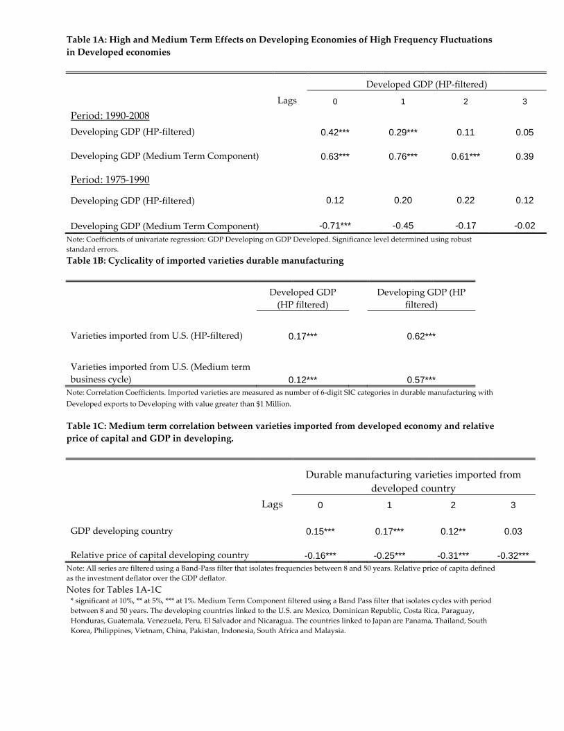
Table 1A: High and Medium Term Effects on Developing Economies of High Frequency Fluctuations

in Developed economies

Developed GDP (HP‐filtered)

Lags 0 1 2 3

Period: 1990‐2008

Developing GDP (HP‐filtered) 0.42*** 0.29*** 0.11 0.05

Developing GDP (Medium Term Component) 0.63*** 0.76*** 0.61*** 0.39

Period: 1975‐1990

Developing GDP (HP‐filtered) 0.12 0.20 0.22 0.12

Developing GDP (Medium Term Component) -0.71*** -0.45 -0.17 -0.02

Note: Coefficients of univariate regression: GDP Developing on GDP Developed. Significance level determined using robust

standard errors.

Table 1B: Cyclicality of imported varieties durable manufacturing

Developed GDP

(HP filtered)

Developing GDP (HP

filtered)

Varieties imported from U.S. (HP‐filtered) 0.17*** 0.62***

Varieties imported from U.S. (Medium term

business cycle) 0.12*** 0.57*** Note: Correlation Coefficients. Imported varieties are measured as number of 6‐digit SIC categories in durable manufacturing with

Developed exports to Developing with value greater than $1 Million.

Table 1C: Medium term correlation between varieties imported from developed economy and relative

price of capital and GDP in developing.

Durable manufacturing varieties imported from

developed country

Lags 0 1 2 3

GDP developing country 0.15*** 0.17*** 0.12** 0.03

Relative price of capital developing country -0.16*** -0.25*** -0.31*** -0.32*** Note: All series are filtered using a Band‐Pass filter that isolates frequencies between 8 and 50 years. Relative price of capita defined

as the investment deflator over the GDP deflator.

Notes for Tables 1A‐1C * significant at 10%, ** at 5%, *** at 1%. Medium Term Component filtered using a Band Pass filter that isolates cycles with period

between 8 and 50 years. The developing countries linked to the U.S. are Mexico, Dominican Republic, Costa Rica, Paraguay,

Honduras, Guatemala, Venezuela, Peru, El Salvador and Nicaragua. The countries linked to Japan are Panama, Thailand, South

Korea, Philippines, Vietnam, China, Pakistan, Indonesia, South Africa and Malaysia.

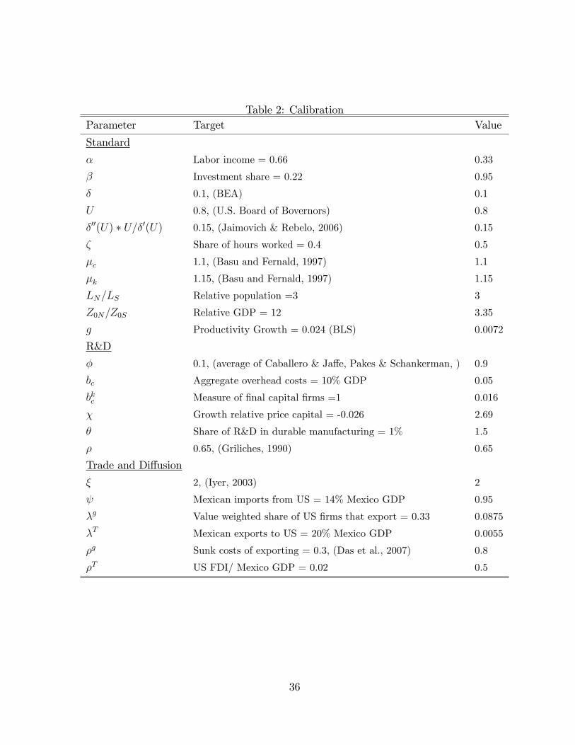
Table 2: CalibrationParameter Target Value

Standard

α Labor income = 0.66 0.33

β Investment share = 0.22 0.95

δ 0.1, (BEA) 0.1

U 0.8, (U.S. Board of Bovernors) 0.8

δ′′(U) ∗ U/δ′(U) 0.15, (Jaimovich & Rebelo, 2006) 0.15

ζ Share of hours worked = 0.4 0.5

µc 1.1, (Basu and Fernald, 1997) 1.1

µk 1.15, (Basu and Fernald, 1997) 1.15

LN/LS Relative population =3 3

Z0N/Z0S Relative GDP = 12 3.35

g Productivity Growth = 0.024 (BLS) 0.0072

R&D

φ 0.1, (average of Caballero & Jaffe, Pakes & Schankerman, ) 0.9

bc Aggregate overhead costs = 10% GDP 0.05

bkc Measure of final capital firms =1 0.016

χ Growth relative price capital = -0.026 2.69

θ Share of R&D in durable manufacturing = 1% 1.5

ρ 0.65, (Griliches, 1990) 0.65

Trade and Diffusion

ξ 2, (Iyer, 2003) 2

ψ Mexican imports from US = 14% Mexico GDP 0.95

λg Value weighted share of US firms that export = 0.33 0.0875

λT Mexican exports to US = 20% Mexico GDP 0.0055

ρg Sunk costs of exporting = 0.3, (Das et al., 2007) 0.8

ρT US FDI/ Mexico GDP = 0.02 0.5

36

Table 3: Volatility Model vs. Data

High Frequency Medium term Cycle

MEXICO Data Model Data Model

GDP 0.026 0.024 0.037 0.045

(0.020, 0.042) (0.029, 0.073)

CONSUMPTION 0.031 0.003 0.040 0.009

(0.003, 0.005) (0.006, 0.014)

INVESTMENT 0.079 0.079 0.082 0.149

(0.067, 0.138) (0.096, 0.242)

RELATIVE PRICE OF

CAPITAL 0.029 0.012 0.042 0.023

(0.011, 0.016) (0.017, 0.031)

IMPORTS (FROM US) 0.090 0.076 0.117 0.141

(0.065, 0.121) (0.086, 0.215)

EXPORTS (TO US) 0.090 0.065 0.134 0.110

(0.059, 0.098) (0.075, 0.168)

TRADE SUPLUS/GDP 0.014 0.014 0.026 0.026

(0.013, 0.024) (0.018, 0.042)

GROWTH IN INTERMEDIATE

GOODS EXPORTED FROM US

TO MEXICO

0.049 (all) 0.047 (dur.)

0.01

(0.006, 0.014)

FDI/GDP 0.004 0.003 0.005 0.012

(0.003, 0.005) (0.007, 0.019)

U.S.

GDP 0.013 0.015 0.015 0.022

(0.014, 0.016) (0.018, 0.025)

CONSUMPTION 0.008 0.006 0.012 0.013

(0.006, 0.007) (0.011, 0.015)

INVESTMENT 0.064 0.089 0.084 0.129

(0.088, 0.097) (0.101, 0.142)

Note: Period 1990‐2006. High frequency corresponds to cycles with periods lower than 8 years and is obtained by filtering simulated

data with a Hodrick‐Prescott filter. Medium term cycles corresponds to cycles with periods shorter than 50 years and is obtained by

filtering simulated data with a Band‐Pass filter. The relative price of capital is the investment deflator divided by the GDP deflator.

Growth in intermediate goods is not filtered. All stands for all manufacturing sectors while dur stands for durable manufacturing.

Table 4: Contemporaneous Co‐movement patterns

PANEL A: Cross‐country correlations between Mexico and U.S.

Data Model

GDP 0.43* 0.72

(0.40, 0.90)

CONSUMPTION 0.20 0.31

(-0.23, 0.72)

PANEL B: Correlation of Mexican Macro Variables with Mexican and U.S. GDP

GDP USA GDP MEXICO

Data Model Data Model

CONSUMPTION 0.02 0.35 0.78*** 0.47

(-0.18, 0.75) (-0.15, 0.87)

INVESTMENT 0.6*** 0.78 0.62*** 0.99

(0.53, 0.92) (0.97, 1.00)

RELATIVE PRICE OF CAPITAL 0.13 -0.90 -0.54*** -0.80

(-0.96, -0.83) (-0.95, -0.52)

IMPORTS (FROM US) 0.61*** 0.84 0.83*** 0.98

(0.62, 0.96) (0.94, 0.99)

EXPORTS (TO US) 0.68*** 0.91 0.08 0.92

(0.79, 0.98) (0.83, 0.97)

MEXICAN TRADE

SURPLUS/GDP 0.07 -0.73 -0.83*** -0.99

(-0.90, -0.42) (-1.00, -0.98)

GROWTH IN INTERMEDIATE

GOODS EXPORTED FROM US

TO MEXICO 0.20 (all)

0.28 (dur.) 0.42 0.35 (all)

0.42 (dur.) 0.36

(0.05, 0.74) (-0.02, 0.68)

FDI/GDP 0.23 0.78 0.11 0.87

(0.54, 0.92) (0.70, 0.97)

Note: Period 1990‐2006. All variables but FDI are scaled by working age population in Mexico. All variables other than growth of

intermediate goods have been HP‐filtered. The model statistics are the average of the contemporaneous cross‐correlations from the

Monte Carlo consisting of 1000 17‐year long simulations. In parenthesis are the 95 percent confidence intervals. The relative price of

capital is measured by the investment deflator over the GDP deflator. All stands for all manufacturing sectors while dur. stands for

durable manufacturing. * denotes significance at the 10% level, ** denotes significance at the 5% level and *** denotes significance at

the 1% level.

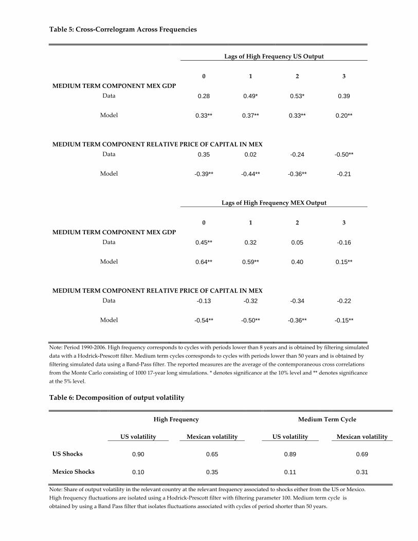
Table 5: Cross‐Correlogram Across Frequencies

Lags of High Frequency US Output

0 1 2 3

MEDIUM TERM COMPONENT MEX GDP

Data 0.28 0.49* 0.53* 0.39

Model 0.33** 0.37** 0.33** 0.20**

MEDIUM TERM COMPONENT RELATIVE PRICE OF CAPITAL IN MEX

Data 0.35 0.02 -0.24 -0.50**

Model -0.39** -0.44** -0.36** -0.21

Lags of High Frequency MEX Output

0 1 2 3

MEDIUM TERM COMPONENT MEX GDP

Data 0.45** 0.32 0.05 -0.16

Model 0.64** 0.59** 0.40 0.15**

MEDIUM TERM COMPONENT RELATIVE PRICE OF CAPITAL IN MEX

Data -0.13 -0.32 -0.34 -0.22

Model -0.54** -0.50** -0.36** -0.15**

Note: Period 1990‐2006. High frequency corresponds to cycles with periods lower than 8 years and is obtained by filtering simulated

data with a Hodrick‐Prescott filter. Medium term cycles corresponds to cycles with periods lower than 50 years and is obtained by

filtering simulated data using a Band‐Pass filter. The reported measures are the average of the contemporaneous cross correlations

from the Monte Carlo consisting of 1000 17‐year long simulations. * denotes significance at the 10% level and ** denotes significance

at the 5% level.

Table 6: Decomposition of output volatility

High Frequency Medium Term Cycle

US volatility Mexican volatility US volatility Mexican volatility

US Shocks 0.90 0.65 0.89 0.69

Mexico Shocks 0.10 0.35 0.11 0.31

Note: Share of output volatility in the relevant country at the relevant frequency associated to shocks either from the US or Mexico.

High frequency fluctuations are isolated using a Hodrick‐Prescott filter with filtering parameter 100. Medium term cycle is

obtained by using a Band Pass filter that isolates fluctuations associated with cycles of period shorter than 50 years.