Dissertation

Medical Tool Tracking in Fluoroscopic InterventionsNew Insights in Detection and Tracking of Tubular Tools

Tim Hauke Heibel

Fakultät für InformatikTechnische Universität München

Computer Aided Medical Procedures(CAMP)

Prof. Dr. Nassir Navab

TECHNISCHE UNIVERSITÄT MÜNCHEN

Fakultät für InformatikComputer-Aided Medical Procedures & Augmented Reality / I16

Medical Tool Tracking in Fluoroscopic InterventionsNew Insights in Detection and Tracking of Tubular Tools

Tim Hauke Heibel

Vollständiger Abdruck der von der Fakultät für Informatik der Technischen UniversitätMünchen zur Erlangung des akademischen Grades eines

Doktors der Naturwissenschaften (Dr. rer. nat.)

genehmigten Dissertation.

Vorsitzender: Univ.-Prof. Dr.-Ing. D. BurschkaPrüfer der Dissertation:

1. Univ.-Prof. Dr. N. Navab

2. Prof. Dr. A. Frangi,Universität Pompeu Fabra, Barcelona, Spain.

Die Dissertation wurde am 23.09.2010 bei der Technischen Universität Müncheneingereicht und durch die Fakultät für Informatik am 11.03.2011 angenommen.

Abstract

These days, fluoroscopic imaging is the modality used most widely to guide physiciansduring minimally invasive abdominal interventions. They involve transarterial chemoem-bolization for hepatocellular carcinoma, the placement of transjugular intrahepatic por-tosystemic shunts or needle aspiration of solitary lung nodules, to name a few. Thesekinds of interventions share the task of navigating a surgical tool to a specific anatomicalsite. Difficulties for the physicians arise from the fact that fluoroscopy, a two-dimensionalmodality, is used to support an actually three-dimensional navigation task. Thus, en-hanced navigation procedures incorporating three-dimensional data are desired for fluo-roscopic interventions. Not only should they improve the navigation but also offer thepotential to reduce treatment time and radiation exposure for the patient as well as thephysician. Due to the complexity of such a system and despite previous efforts, an inte-grated solution does not yet exist.

Localization of medical tools and the estimation of their motion are core componentsof such a navigation system and this work focuses on related methods to improve thedetection and tracking during fluoroscopic interventions.

To this end, different image enhancement algorithms required for the tool localizationare reviewed and analyzed in a unified framework. Based on the analysis a fast androbust localization scheme is developed. Furthermore, a novel method for tracking thetools in a non-rigid environment is introduced. The tracking algorithm is based on discreteoptimization and thus it is derivative free and can deal with complex models. It is fastand robust and hence complying with application specific constraints. Moreover, thepresented tracking method is generic and can be extended to closed curves, which makesit applicable to other problems such as segmentation.

Based on the results, a novel respiratory motion estimation procedure is developed. Itis the basis for the creation of a navigation system and is essential in order to establishthe relation between the location of medical tools and three-dimensional data used forthe actual navigation.

Keywords:Biomedical Image Processing, Image-Guided Interventions, Optical Tracking,Computer-Aided Navigation

Zusammenfassung

Durchleuchtung ist heutzutage die Modalität der Wahl, um Ärzte bei der Navigati-on während minimal-invasiven Eingriffen zu unterstützen. Abdominelle, minimal-invasiveEingriffe sind vielfältig und umfassen transarterielle Chemo-Embolisation (TACE) beiHepatocellular carcinoma (HCC), die Platzierung von transjugulären intrahepatischenportosystemischen Shunts (TIPS) oder auch die Punktion einzelner Knoten der Lun-ge, um nur einige zu nennen. Eine Gemeinsamkeit dieser Art von Interventionen ist es,dass der behandelnde Arzt während des Eingriffs ein interventionelles Werkzeug zu einerbestimmten anatomischen Stelle, dem sogenannten Situs, navigieren muss. Schwierigkei-ten bei der Navigation entstehen dadurch, dass zur Unterstützung bei dieser tatsächlichdreidimensionalen Navigationsleistung Durchleuchtung, also eine zweidimensionale Mo-dalität verwendet wird. Demzufolge ist die Entwicklung einer verbesserten Navigations-unterstützung erstrebenswert, die im besten Fall etwaige vorhandene, dreidimensionaleDaten nutzt. Diese Verbesserungen sollen nicht nur die Navigation vereinfachen, sondernmöglichst auch Interventionszeiten verkürzen und damit die Belastung durch Röntgen-strahlung und dies sowohl für den behandelnden Arzt als auch den Patienten. Aufgrundder Komplexität solch eines Systems gibt es trotz verschiedenster Bemühungen bis heutenoch keine in den klinischen Alltag integrierte Lösung.

Die Lokalisierung medizinischer Instrumente und die Bestimmung ihrer Bewegung sindzentrale Komponenten eines solchen Navigationssystems. Diese Arbeit beschäftigt sichmit Möglichkeiten zur Verbesserung von Methoden zur Detektion und dem sogenanntenTracking medizinischer Instrumente in Durchleuchtungssequenzen.

Zu diesem Zweck werden verschiedene Algorithmen zur Hervorhebung und Detektionvon medizinischen Werkzeugen untersucht und in einem einheitlichen Framework analy-siert. Basierend auf der Analyse, wird ein robustes Verfahren zur Detektion erarbeitet.Desweiteren wird in dieser Arbeit ein neuartiges Verfahren zum Tracking nicht-linearerBewegungen von interventionellen Geräten beschrieben. Das Tracking-Verfahren ist nichtgradientenbasiert und erlaubt deshalb die Verwendung komplexer Modelle. Desweiterenist das Verfahren effizient und entspricht somit strengen den Anforderungen der interven-tionellen Radiologie.

Basierend auf den Ergebnissen, wird ein neues Verfahren zur Bestimmung der Atem-bewegung entwickelt. Es bildet die Basis für zukünftige Navigationssysteme und ist not-wendig, um eine Beziehung zwischen zweidimensionalen Positionen von Werkzeugen undden dreidimensionalen Datensätzen für die eigentliche Navigation herzustellen.

Schlagwörter:Biomedizinische Bildverarbeitung, Bildgestützte Interventionen, Optisches Tracking,Computerunterstützte Navigation

Acknowledgments

First of all, I would like to thank Nassir Navab for his continuous support. His highlymotivating spirit, his interest in the field of medical computer science and his attitudetowards scientific research inspired and helped me a lot. Without his feedback and inspi-ration this work would not have been possible.

I also owe thanks to the Siemens Healthcare Angiography/X-Ray division (Forchheim,Germany) for their financial support. In particular I would like to thank Markus Pfisterand Klaus Klingenbeck for their continuous support during my work.

I would also like to thank the people from CAMP for their part in creating the researchfriendly environment which I had the pleasure to work within. In particular, I would liketo thank Ben Glocker for the many hours in which we discussed various problems on dis-crete optimization, in which we worked jointly on tracking, registration and segmentationproblems and for the fun we had in our spare time. I also want to thank Darko Zikic, An-dreas Keil, Olivier Pauly and Max Baust for the many fruitful discussions we had and thejoint work we did together. Many thanks got to Marco Feuerstein and especially MartinGroher. Not only did they take vast amounts of work from my shoulders during the timein which I was writing my thesis but they always supported me with valuable feedbackand their joint scientific experience. To all of you and those I did not mention, I wouldlike to say thank you once more. You have made writing my thesis a great experienceand have become more than mere co-workers.

I am much obliged to my family, my brother and especially my mother who supportedme throughout my whole studies making this thesis at all possible. Last but not least, Iwould like to thank my beloved wife Elena. You have endured most of all and stood bymy side the whole time, encouraging me when I lacked courage, cheering my up when Iwas not cheerful and listening to me when I needed to talk. You are the cornerstone ofthis work.

Without any of you this thesis would not have been possible.

This work is dedicated to my father.Dr. med. Jörg-H. Heibel

(January 18, 1949 – May 28, 1998)

vii

CONTENTS

Thesis Outline 1

1 Interventional Radiology and Navigation Procedures 51.1 Introduction . . . . . . . . . . . . . . . . . . . . . . . . . . . . . . . . . . . 51.2 Clinical Routine . . . . . . . . . . . . . . . . . . . . . . . . . . . . . . . . . 5

1.2.1 Imaging Modalities . . . . . . . . . . . . . . . . . . . . . . . . . . . 61.3 Problem Statement . . . . . . . . . . . . . . . . . . . . . . . . . . . . . . . 101.4 A Navigation System for Fluoroscopic Interventions . . . . . . . . . . . . . 11

1.4.1 Motion Compensation Module Details . . . . . . . . . . . . . . . . 14

2 Previous Work 192.1 Enhancement of Tubular Structures . . . . . . . . . . . . . . . . . . . . . . 19

2.1.1 Scale-Space Theory . . . . . . . . . . . . . . . . . . . . . . . . . . . 212.2 Detection of Guide-Wires and Needles . . . . . . . . . . . . . . . . . . . . 222.3 Tracking of Guide-Wires and Needles . . . . . . . . . . . . . . . . . . . . . 28

3 Tool Detection 333.1 Modeling Tubular Tools . . . . . . . . . . . . . . . . . . . . . . . . . . . . 33

3.1.1 X-ray Attenuation . . . . . . . . . . . . . . . . . . . . . . . . . . . 333.1.2 An Idealized Tube Model . . . . . . . . . . . . . . . . . . . . . . . . 343.1.3 Typical Tube Models . . . . . . . . . . . . . . . . . . . . . . . . . . 36

3.2 Enhancement of Tubular Structures . . . . . . . . . . . . . . . . . . . . . . 393.2.1 Differential Geometry in Image Processing . . . . . . . . . . . . . . 403.2.2 The Hessian and its Relation to Tube Models . . . . . . . . . . . . 433.2.3 Properties of Tube Enhancement Filters . . . . . . . . . . . . . . . 44

3.3 Semi-Automatic Detection . . . . . . . . . . . . . . . . . . . . . . . . . . . 533.4 Fully Automatic Detection . . . . . . . . . . . . . . . . . . . . . . . . . . . 58

3.4.1 Canny Ridge Detection . . . . . . . . . . . . . . . . . . . . . . . . . 583.4.2 Steger Ridge Detection . . . . . . . . . . . . . . . . . . . . . . . . . 60

3.5 Discussion . . . . . . . . . . . . . . . . . . . . . . . . . . . . . . . . . . . . 62

ix

CONTENTS

4 Tool Tracking 654.1 Modeling of Guide-Wires and Needles . . . . . . . . . . . . . . . . . . . . . 664.2 Modeling of Objective Functions . . . . . . . . . . . . . . . . . . . . . . . . 694.3 Markov Random Fields for Tracking . . . . . . . . . . . . . . . . . . . . . 74

4.3.1 Optimization . . . . . . . . . . . . . . . . . . . . . . . . . . . . . . 774.4 Experiments and Evaluation . . . . . . . . . . . . . . . . . . . . . . . . . . 78

4.4.1 Error Assessment . . . . . . . . . . . . . . . . . . . . . . . . . . . . 784.4.2 Approximation Error . . . . . . . . . . . . . . . . . . . . . . . . . . 794.4.3 Deformation Space Discretization . . . . . . . . . . . . . . . . . . . 804.4.4 Experiments on clinical data . . . . . . . . . . . . . . . . . . . . . . 82

5 A Simplified Motion Compensation System 875.1 Plugin Design . . . . . . . . . . . . . . . . . . . . . . . . . . . . . . . . . . 875.2 Visualization Component . . . . . . . . . . . . . . . . . . . . . . . . . . . . 89

6 Conclusion 936.1 Discussion . . . . . . . . . . . . . . . . . . . . . . . . . . . . . . . . . . . . 946.2 Future Work . . . . . . . . . . . . . . . . . . . . . . . . . . . . . . . . . . . 95

A Authored and Co-Authored Publications 99

B Mathematical Extensions 101B.1 Enhancement of Tubular Structures . . . . . . . . . . . . . . . . . . . . . . 101

B.1.1 Sato’s and Frangi’s Feature Enhancement . . . . . . . . . . . . . . 101B.1.2 Koller’s Feature Enhancement . . . . . . . . . . . . . . . . . . . . . 102

C Code Samples 103

List of Figures 105

References 107

Abbreviations 115

x

Thesis Outline

Minimally invasive procedures, in particular endovascular interventions have becomeclinical routine. The common task of these procedures is to navigate a medical tool likea needle or a guide-wire to an intervention situs. During this navigation task, physicianshave access to instant visual feedback in form of an X-ray image stream. Besides theimage data the interventionalists are solely relying on their knowledge of anatomicalstructures as well as haptic feedback. The actual three-dimensional pose of the toolsneeds to be currently reconstructed mentally. In case of endovascular interventions themental reconstruction has to be regularly verified by injecting contrast agent into theX-ray transparent vasculature.A possible way to aid physicians in this task is an improved three-dimensionalnavigation system. Two core components such a system requires are the localization andmotion estimation of medical tools. Localization refers to the problem of detecting amedical tool in the images without prior information regarding its location. During themotion estimation or tracking task on the other hand side the system is initialized withthe previous position of the medical tool. This prior knowledge simplifies the trackingproblem such that automatic methods that require no user interaction can be designedthough this is not yet possible for the tool detection. A complete navigation systemrequires more components which are described in detail in Section 1.4.Difficulties with these techniques arise from the fact that as a consequence of the lowenergy X-rays, the images usually exhibit a low signal to noise ratio (SNR).Furthermore, since needles and guide-wires are thin one-dimensional structures, they areoftentimes hard to distinguish from the cluttered anatomical background. For trackingguide-wires and catheters another problem that arises is the highly non-linear motionthe tools undergo. This is caused by patient breathing, different motions at organinterfaces, interactions of the physician, and perspective projection of transparentstructures. Together, these issues make the motion estimation problem in X-rayfluoroscopy extremely difficult.To be accepted by physicians, ease of use is an important requirement for a navigationsystem. In the optimal case it would not be interfering or changing existing work-flowsand it would not rely on user input from the physicians. So far, no such system existswhich is robust enough for every day clinical use. Especially the detection still requiresuser interactions. Another requirement is the real-time capability of a navigationsystem. Fast processing is required to keep the time intervals between observationssmall and because other modules belonging to a navigation system require computationtime as well. In summary, a navigation system should be capable of robustly handlinglow-quality image data, requiring minimal user interaction and operating near real-time.This thesis presents novel concepts to support physicians in their navigation task duringfluoroscopic interventions. The work evaluates and revisits methods required to build athree-dimensional navigation system. The focus of this work lies on the detection andtracking components. In particular a novel scheme for deformable tracking of curvilineartools such as guide-wires and needles in fluoroscopic X-ray sequences is derived andevaluated.

1

In the following, we give a brief outline and summary of the thesis and its chapters.

Chapter 1: Fluoroscopic Interventions and Navigation Procedures The firstchapter provides an overview of fluoroscopy guided interventions. Problems physiciansare facing and which can potentially be overcome or minimized by computer aidedsystems are discussed in detail. Furthermore, different imaging modalities used duringsuch procedures are introduced. These image modalities are of significant importance.First, their understanding gives insights to many problems involved in the design anddevelopment of a navigation system. Second, imaging modalities are not alwaysimposing problems but sometimes enable new ways of visualizations which are nowadaysnot used to their full potential. In the end, a navigation system for fluoroscopicinterventions is presented. The required components of such a system are discussed andan example of the working system is given.

Chapter 2: Previous Work After introducing the problem and a potential solution,Chapter 2 gives an overview of the related work. It is divided in three sections where atfirst image enhancement methods for tubular or curvilinear structures are discussed.These methods are required because of the degraded image quality caused by low energyX-rays. A summary of existing tool detection methods follows this section. The sectionpresents methods from various fields, not necessarily interventional imaging. A lot ofresearch has focused on the detection of curvilinear structures which can be streets fromaerial images and vessels or medical tools from clinical image data. The last sectionpresents the related work on tracking methods. The approaches to solve the trackingproblem can be categorized in two main branches. One branch is tackling the problemwith methods driven by image features and a second branch uses approaches which arebased on learned data.

Chapter 3: Tool Detection Chapter 3 on tool detection presents a novelsemi-automatic strategy for medical tool delineation. The presented method is based onstructural information contained in the second-order derivatives of image intensities andshortest-paths in a graph induced by the structural information. At first themathematical properties of tools and their imaging process are presented in Section 3.1.This follows a detailed discussion and comparison of enhancement techniques of tubularstructures and their mathematical formulations. Section 3.3 presents the actual methodfor tool delineation. An overview of fully automatic methods is given in Section 3.4. Itpresents two methods that can be used for the automatic generation of point setsrepresenting line-like structures and discusses the limitations of these methods. The lastSection 3.5 summarizes issues related to semi- and fully automatic methods and presentsearly ideas of what is required for the successful implementation of fully automaticdetection schemes which are clinically applicable.

Chapter 4: Tool Tracking The main focus of the thesis is a novel scheme for thetracking of medical tools. The method is presented in Chapter 4 which is divided inseveral sub-sections. The first one, Section 4.1 presents how to model medical tools and

2

their shapes mathematically. It also presents how tool motions are modeled andprovides a scheme for their efficient evaluation. In Section 4.2 the objective functionthat defines the optimization process of the motion estimation is presented. Objectivefunctions typically contain two components – a so called external energy which drivesthe optimization process and a second one, called internal energy which imposes softconstraints on the solutions. Choices for modeling internal energies are various anddiscussed separately. After the energy function is defined, Section 4.3 presents how tomodel the problem in a discrete framework in which the result is computed as amaximum a posteriori (MAP) estimate of a Markov random field (MRF) formulation.Experiments are part of the last section of this chapter. Section 4.4 containsexperiments on various synthetic as well as clinical sequences. Different experiments areused to evaluate different aspects of the proposed solution and serve to support thedesign of the final system.

Chapter 6: Conclusion The presented methods are not solving all issues occurringduring the detection and tracking of medical tools. The last chapter summarizes thework and discusses unsolved problems and parts that require further improvements inSection 6.1. The final part of the thesis, Section 6.2 provides novel ideas which can leadto further improvements during the detection and tracking. In particular it will discussthe feasibility of the integration of learning based methods into a MRF framework andprovide an example of such a method.

3

CHAPTER

ONE

INTERVENTIONAL RADIOLOGY AND NAVIGATIONPROCEDURES

1.1 IntroductionInterventional radiology is a medical branch in which diseases are treated minimallyinvasive using image guidance. To this end, physicians introduce small catheters,catheter-based devices or needles percutaneously without the need for surgery or generalanesthesia. Application fields for minimally invasive procedures and in particularendovascular interventions are various and range from diagnostic (e.g, needle biopsies)over treatment (e.g., percutaneous transluminal angioplasty) to palliative (e.g.,transarterial chemoembolization) purposes.The common task in these procedures is to navigate a medical tool like a needle or aguide-wire to an intervention situs. This guidance task is mainly supported throughdifferent imaging modalities which provide visual feedback for the interventionalist.Along with the visual information physicians rely on their three-dimensional knowledgeof anatomical structures as well as haptic feedback while tools are steered towards thedesired area of interest.Many cases which required surgical treatment in earlier days can today be treatednon-surgically. The minimally invasive treatment results in reduced risk for the patient.It causes less physical trauma and leads to reduced infection rates, improved recoverytime and shortened hospital stays.

1.2 Clinical RoutineImage-guided and in particular endovascular interventions have become clinical routine.Various procedures exist and they serve diagnostic, therapeutic and palliative purposes.Some common treatments are the transjugular intrahepatic portosystemic shunt (TIPS)placement, endovascular stent placement in case of abdominal aortic aneurysms (AAAs),needle biopsies and transarterial chemoembolization (TACE) to deal with hepatocellularcarcinoma (HCC). The common difficulty during these procedures is the placement of a

5

medical tool in the human vascular system. In interventional radiology this task isimage guided and the physicians can be supported by various imaging modalities.Diagnosis and planning of interventions is generally supported by images of the patient.Since these images are acquired before the intervention, they are referred to aspre-interventionally acquired images. This kind of images is usually characterized byhigh quality and consequently high X-ray dose exposure. The dimensionality of imagesvaries between 2D (e.g., chest X-ray) and 3D (e.g., magnetic resonance tomography(MRT) or computed tomography (CT)).During interventions, physicians have access to so called intra-interventional images andagain 2D and 3D images are used. Because it is important to reduce the radiationexposure during procedures, lower doses are common which results in degraded imagequality (i.e. a low SNR). In interventional radiology fluoroscopic image sequences aremost common. Their purpose is to monitor patient anatomy and the assessment ofmedical tool positions during the exam.Not all image data used during interventions is of low quality. Two exceptions aredigital subtraction angiographys (DSAs) and 3D rotational angiographys (3D-RAs).DSAs are commonly used and they mostly serve as roadmaps because fluoroscopicimages show vasculature only when contrast agent (typically iodine based) is injectedinto the vessel system. Three dimensional image data such as 3D-RA on the other handis more seldom used. The acquisition requires relatively high X-ray doses and also muchcontrast dye application to visualize the patient’s vessel anatomy. 3D angiograms can beused to diagnose diseases (e.g., stenosis), for the verification of interventions (e.g., afterballoon angioplasties) and also as roadmaps. Both modalities, DSA and 3D-RA, do notcapture patient motion nor temporal changes of instrument locations which means theyare not directly1 usable for navigation purposes.The imaging modalities mentioned above are the most common during endovascularinterventions. Especially for needle interventions other modalities exist as well, inparticular ultrasound is used oftentimes to guide the physician. Image properties andtheir corresponding acquisition processes, which are of most interest in this work, will bedescribed in more detail in the next section.

1.2.1 Imaging ModalitiesFluoroscopy

One of the most common imaging techniques used in interventional radiology isfluoroscopy. The method provides physicians with a real-time X-ray “movie” of thepatient’s internal structures. Typical acquisition rates for fluoroscopy are 3.5, 7.5, 15and 30 (continuous fluoroscopy) frames per second. Fluoroscopic imaging is used tomonitor instruments like catheters, organ movement, and vessel structures if combinedwith contrast injection.Even though, compared to classic radiography, physicians use low dose rates duringfluoroscopies, the overall absorbed dose can become relatively high due to the large

1Indirectly, because they are oftentimes used as roadmaps.

6

amount of images being acquired and the length of the procedure. The introduction offlat-panel detectors instead of formerly common image intensifiers lessens the problembut the procedure still requires careful balancing between risk and potential gain.

Images acquired during fluoroscopy oftentimes suffer from a low SNR. This appears asgraining on the image and is caused by the low dose used for the image acquisition. Thehigh noise level in fluoroscopy is one of the major limiting factors hampering objectdetection and it is directly affecting image processing in interventional radiology.

(a) Standard chest X-ray showing a catheterand no vasculature.

(b) Angriogram of liver vessels.

(c) Digital Subtraction Angiography. (d) Fluoroscopy showing a magnification ofa catheter and guide-wire.

Figure 1.1: Most common 2D image modalities in interventional radiology.

7

Angiography

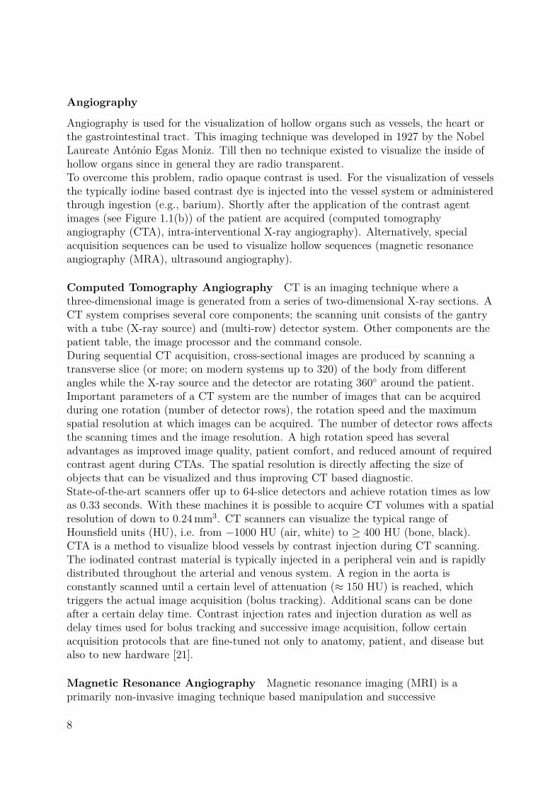
Angiography is used for the visualization of hollow organs such as vessels, the heart orthe gastrointestinal tract. This imaging technique was developed in 1927 by the NobelLaureate António Egas Moniz. Till then no technique existed to visualize the inside ofhollow organs since in general they are radio transparent.To overcome this problem, radio opaque contrast is used. For the visualization of vesselsthe typically iodine based contrast dye is injected into the vessel system or administeredthrough ingestion (e.g., barium). Shortly after the application of the contrast agentimages (see Figure 1.1(b)) of the patient are acquired (computed tomographyangiography (CTA), intra-interventional X-ray angiography). Alternatively, specialacquisition sequences can be used to visualize hollow sequences (magnetic resonanceangiography (MRA), ultrasound angiography).

Computed Tomography Angiography CT is an imaging technique where athree-dimensional image is generated from a series of two-dimensional X-ray sections. ACT system comprises several core components; the scanning unit consists of the gantrywith a tube (X-ray source) and (multi-row) detector system. Other components are thepatient table, the image processor and the command console.During sequential CT acquisition, cross-sectional images are produced by scanning atransverse slice (or more; on modern systems up to 320) of the body from differentangles while the X-ray source and the detector are rotating 360 around the patient.Important parameters of a CT system are the number of images that can be acquiredduring one rotation (number of detector rows), the rotation speed and the maximumspatial resolution at which images can be acquired. The number of detector rows affectsthe scanning times and the image resolution. A high rotation speed has severaladvantages as improved image quality, patient comfort, and reduced amount of requiredcontrast agent during CTAs. The spatial resolution is directly affecting the size ofobjects that can be visualized and thus improving CT based diagnostic.State-of-the-art scanners offer up to 64-slice detectors and achieve rotation times as lowas 0.33 seconds. With these machines it is possible to acquire CT volumes with a spatialresolution of down to 0.24 mm3. CT scanners can visualize the typical range ofHounsfield units (HU), i.e. from −1000 HU (air, white) to ≥ 400 HU (bone, black).CTA is a method to visualize blood vessels by contrast injection during CT scanning.The iodinated contrast material is typically injected in a peripheral vein and is rapidlydistributed throughout the arterial and venous system. A region in the aorta isconstantly scanned until a certain level of attenuation (≈ 150 HU) is reached, whichtriggers the actual image acquisition (bolus tracking). Additional scans can be doneafter a certain delay time. Contrast injection rates and injection duration as well asdelay times used for bolus tracking and successive image acquisition, follow certainacquisition protocols that are fine-tuned not only to anatomy, patient, and disease butalso to new hardware [21].

Magnetic Resonance Angiography Magnetic resonance imaging (MRI) is aprimarily non-invasive imaging technique based manipulation and successive

8

measurements of magnetic fields in the body. Because the method is not relying onionizing radiation the imaging technique is not harmful for the patient in terms of X-rayexposure. Opposed to CT, MRI offers better contrast between different types of softtissue which makes it useful for various clinical problems and in particular vascular andcardio-vascular imaging.During the imaging process a strong magnetic field is used to align protons in the body.Once the protons are aligned, radio frequency (RF) fields (i.e., electromagnetic fields)are used to systematically change this alignment. When the fields are deactivated, theprotons fall back into their original spin-state and the energy difference between the twostates causes the release of photons with a specific frequency and energy. These photonsare then measured by the magnetic resonance (MR) detector and the physicalrelationship between the field-strength and photon’s frequency allows to use the processfor imaging. Different tissues can be distinguished since protons return to theirequilibrium state at different rates, which can be measured too. In order to determinethe spatial location of the signals, magnetic field gradients are applied for slice selection,row selection (phase encoding), and column selection (frequency encoding).There are several MRA techniques, some of them involving a contrast injection as CTA.Here, however, the contrast has to be paramagnetic extracellular, e.g. gaudolinium.There are also fully non-invasive techniques for angiographic MR imaging by using theflow property of blood (Time-of-Flight MRA, Phase-Contrast MRA). See Figure 1.2 foran example of contrasted CTA and MRA slices.

Figure 1.2: Computed Tomography Angiography (left) and Magnetic Resonance Angiog-raphy (right).

Cone-Beam Computed Tomography Angiography Cone-Beam CT which is alsoreferred to as helical (or spiral) cone-beam CT is a technique in which an X-ray sourcerotates around the patient while acquiring a set of radiographies. Mathematicalmethods such as the filtered back projection (FBP) or algebraic reconstructiontechnique (ART) [37] can be used to reconstruct a three-dimensional representation of

9

the patient. The image acquisition can e.g. be performed with a modern C-arm systemin which the gantry is attached to a robot controlled arm which allows positioning withsix degrees of freedom. Alternatively, smaller and mobile C-arm systems exist whichallow to bring this technique into any intervention room or the operation theater.The advantages of cone-beam CT include a reduced scan-time, dose reduction as well asimproved image quality and reduced cost compared to conventional CT. From aninterventionalist’s point of view another improvement is that it is possible to perform theimage acquisition in the intervention room without being required to move the patient.Cone-Beam CTAs (sometimes also called 3D-RA or 3D X-ray angiography (3DXA)) areacquired by performing the image generation after the application of iodine basedcontrast agent. As it is common for other angiographic exams, the contrast agent iseither injected or ingested.

1.3 Problem StatementThis section presents which problems physicians and patients are facing duringendovascular interventions. Transarterial chemoembolizations (TACEs) serves as anexemplary procedure performed by interventionalists on a daily basis.Hepatocellular carcinomas (HCCs) are a common disease (cancer) of the liver. TACE isusually performed on unresectable tumors. It is done as a safe palliative treatment orwhile patients are waiting for a liver transplant. During the procedure a mixture of anantineoplastic drug, an embolic agent and radio opaque contrast agent is inserted intothe vessels feeding the liver tumor.While the physician is performing the intervention, he inserts a guide-wire into thefemoral artery in the groin. From there, the guide-wire is advanced through the aortavia the truncus coeliacus into the arteria hepatica communis and from there into thevessels feeding the actual tumor where the embolic mixture is released. Steering the

Figure 1.3: Angiographic intervention setup. The monitor shows a live X-ray video stream(left) next to a DSA (right) which serves as a roadmap during the intervention. The objecton the left-hand side of the image is a flat-panel detector from a modern C-arm system.

10

guide-wire involves passing through several vessel branches and the main difficulty is thefact that blood vessels are radio transparent. The immediate question arising is howinterventionalists deal with this difficult situation.TACE is performed under angiographic image guidance. It is common that at first,when the patient is entering the intervention room, a cone-beam CTA is generated toassess the exact location at which the embolic mixture should be released. Next, a DSA(see Figure 1.3, right image on the monitor) is generated which serves as a roadmapduring the navigation task. The actual procedure is performed under constantangiographic surveillance (see Figure 1.3, left image on the monitor). Whenever thephysician assumes to be close to a branching point contrast dye is release to visualizethe vessel structures in the vicinity of the catheter tip and in order to determine thenext steps. The catheter itself is advanced along the guide-wire. When the interventionsitus is reached the chemicals are released and the guide-wire and catheter areextracted. A standard system setup can be seen in Figure 1.3.The current procedure involves several problems. First, it requires much experience ofthe interventionalist to perform the procedure in a relatively short time – and time iscrucial due to the constant expose to ionizing radiation. Second, the physician needs tomentally transfer the observed flow information as perceived when injecting contrastagent to the roadmap to be able to correctly assess the current guide-wire and cathetertip location. There exist also problems related to the 2D imaging modalities used tosupport the navigation task. When a vessel branch is aligned with the projectiondirection spacial information is lost, because all 3D locations along that branch projectonto the same 2D image location. There is no way of assessing the tool depth and insuch a scenario, the physician must change the whole imaging setup and acquire a newDSA since it is only valid for a specific C-arm configuration.The intention of this work is to provide solutions and new insights required to create anovel navigation system aiding physicians during endovascular procedures. Such asystem should aim at improving the overall navigation. It should prevent the need forsuccessive image acquisitions, the need for system reconfigurations (e.g., C-armangulation) and thus reduce the intervention time and the involved exposure to ionizingradiation.

1.4 A Navigation System for FluoroscopicInterventions

In order to support physicians during endovascular procedures, various researchers havecome up with a variety of proposals. These can generally be classified into two differentapproaches – those using a roadmap while trying to overlay it onto a fluoroscopic imagesequence [73, 52, 53, 38, 25, 1] and those trying to utilize a 3D-RA to directly annotatethe tool locations in 3D [77, 8, 27]. Both approaches rely on establishing a spatialrelationship between the fluoroscopic sequence and either a roadmap or a 3D-RA. Oneof the main problems aggravating the development of navigation systems is the dynamicnature of this relationship.

11

The methods aiming at blending the fluoroscopic sequence with a roadmap require theC-arm projection geometry to be known. The imaging parameters consists of intrinsicparameters as source to image distance (SID), pixel size and field of view (FOV) as wellas extrinsic parameters, i.e. the C-arm orientation. Given the projection parameters, itis now possible to create the roadmap image by either creating a projection of a 3D-RAor by generating a DSA. Assuming furthermore a static scenario where the patient doesnot move (breathing, heart-beat) these roadmaps can directly be mixed with thefluoroscopic sequence because all data is generated under the same projection. Formerresearch has focused primarily on precision analysis [73, 52] as well as the effects ofimage distortion [55, 68].The second method is based on annotating guide-wire or catheter positions directly in3D. Here, one needs to establish a spatial relationship between the two-dimensionalfluoroscopic sequence and a three-dimensional data set such a CTA or a 3D-RA. Twoways to achieve this have been pursued so far – one approach based on biplane C-armsystems [2] and a second method which tries to compute the 3D locations from only asingle view [77, 8, 27].A common problem during the realization of such navigation systems is the dynamicnature of the observed scenes where patient breathing and heart-beat are two exemplarycauses. The motion is problematic because it is not reflected in the static,pre-operatively acquired image data (e.g. DSA, 3D-RA) that is used by theinterventionalists during the procedures. Dealing with the motion requires so calledtracking techniques for both approaches, those using roadmaps and those annotating

Registration

DSA – Fluoro

2D – 3D

Registration

Robust

Backprojection

3D Vessel Model

Motion

Compensation

Figure 1.4: Components of interventional navigation.

12

tool positions in three-dimensional image data.In the remainder of this section we will focus on the approach offering three-dimensionaltool annotations and provide a detailed overview of the required components for such asystem. In general, endovascular scenarios cannot be assume to be static – tools aremoving and bending and patients are breathing, exhibit cardiac activity and areoftentimes moving. Therefore, it is desired that a navigation system is capable ofdealing with such situations. It should be designed such that dynamic and non-linearprocesses can be modeled and captured. Ignoring the image acquisition, such a flexiblenavigation system requires 4 main components.

1. Deformable 2D-3D Registration Module: This module is required toestablish a spatial relationship between the two-dimensional roadmap (e.g. DSA)and the three-dimensional image data (e.g. 3D-RA). Literature dealing with thisproblem (e.g. [26, 29]) is still limited because the task is severely ill-posed. Givenonly a single view, it is not possible to assess displacements in the projectiondirection, i.e. in z-direction of the camera coordinate system. Theoretically, thisleads to an infinite number of possible solutions for such a registration and thussuch a system requires (soft) constrained optimizations processes. Lengthpreservation and deformation smoothness are two common ways of constrainingsuch a process. This module is depicted on the right in Figure 1.4 and labeled as“2D-3D Registration”.

2. Deformable 2D-2D Registration Module: The deformable registrationbetween a key-frame from the two-dimensional fluoroscopic sequence and thetwo-dimensional DSA allows to relate pixel positions in the key-frame to positionsin the DSA. This is an important step because so far, only the relation betweenthe DSA and the 3D-RA has been established but not the relation between thefluoroscopic sequence and the 3D-RA. To our best knowledge, this particularproblem has not yet been addressed by any researcher but it is likely that existing2D-2D registration methods such as [24] could be used to perform this task. It isnot even clear, whether a deformable registration is required at this step when theDSA is acquired under the same projection as the fluoroscopic image sequence.Given that the apparent motion observed in fluoroscopic videos is cyclic, thereexists a key-frame in the image sequence which was acquired in a similar cardiacphase as the DSA and therefore offers maximal similarity. Furthermore, DSAs aregenerated from two X-ray images – one with and another one without contrastagent. The contrast free X-ray image is of the same modality as the fluoroscopickey-frame which is another indicator that such a registration should be feasible.The module is depicted at the bottom of Figure 1.4 and labeled as “RegistrationDSA-Fluoro”.

3. Motion Compensation Module: The motion compensation is the componentencapsulating the main contribution of this work. Compensation of apparentmotion is required because the fluoroscopic video sequence is not static. Patientbreathing and heart-beat as well as tool interactions performed by the physicians

13

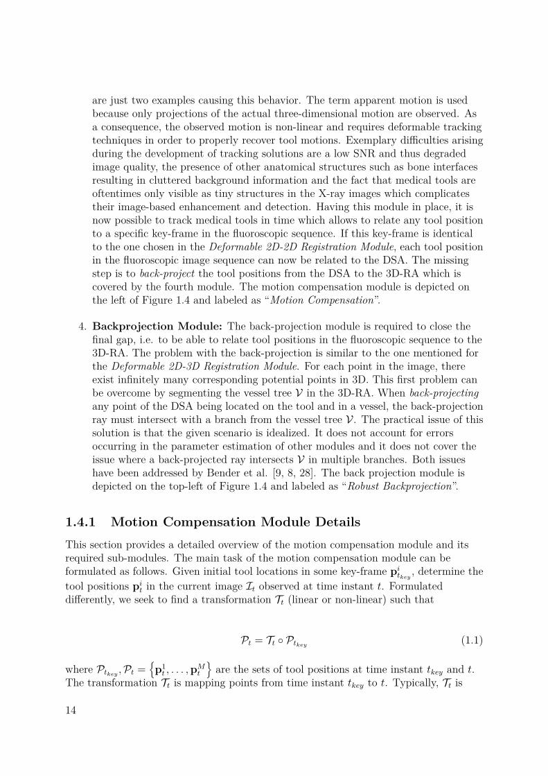
are just two examples causing this behavior. The term apparent motion is usedbecause only projections of the actual three-dimensional motion are observed. Asa consequence, the observed motion is non-linear and requires deformable trackingtechniques in order to properly recover tool motions. Exemplary difficulties arisingduring the development of tracking solutions are a low SNR and thus degradedimage quality, the presence of other anatomical structures such as bone interfacesresulting in cluttered background information and the fact that medical tools areoftentimes only visible as tiny structures in the X-ray images which complicatestheir image-based enhancement and detection. Having this module in place, it isnow possible to track medical tools in time which allows to relate any tool positionto a specific key-frame in the fluoroscopic sequence. If this key-frame is identicalto the one chosen in the Deformable 2D-2D Registration Module, each tool positionin the fluoroscopic image sequence can now be related to the DSA. The missingstep is to back-project the tool positions from the DSA to the 3D-RA which iscovered by the fourth module. The motion compensation module is depicted onthe left of Figure 1.4 and labeled as “Motion Compensation”.

4. Backprojection Module: The back-projection module is required to close thefinal gap, i.e. to be able to relate tool positions in the fluoroscopic sequence to the3D-RA. The problem with the back-projection is similar to the one mentioned forthe Deformable 2D-3D Registration Module. For each point in the image, thereexist infinitely many corresponding potential points in 3D. This first problem canbe overcome by segmenting the vessel tree V in the 3D-RA. When back-projectingany point of the DSA being located on the tool and in a vessel, the back-projectionray must intersect with a branch from the vessel tree V . The practical issue of thissolution is that the given scenario is idealized. It does not account for errorsoccurring in the parameter estimation of other modules and it does not cover theissue where a back-projected ray intersects V in multiple branches. Both issueshave been addressed by Bender et al. [9, 8, 28]. The back projection module isdepicted on the top-left of Figure 1.4 and labeled as “Robust Backprojection”.

1.4.1 Motion Compensation Module DetailsThis section provides a detailed overview of the motion compensation module and itsrequired sub-modules. The main task of the motion compensation module can beformulated as follows. Given initial tool locations in some key-frame pitkey , determine thetool positions pit in the current image It observed at time instant t. Formulateddifferently, we seek to find a transformation Tt (linear or non-linear) such that

Pt = Tt Ptkey (1.1)

where Ptkey ,Pt =p1t , . . . ,pMt

are the sets of tool positions at time instant tkey and t.

The transformation Tt is mapping points from time instant tkey to t. Typically, Tt is

14

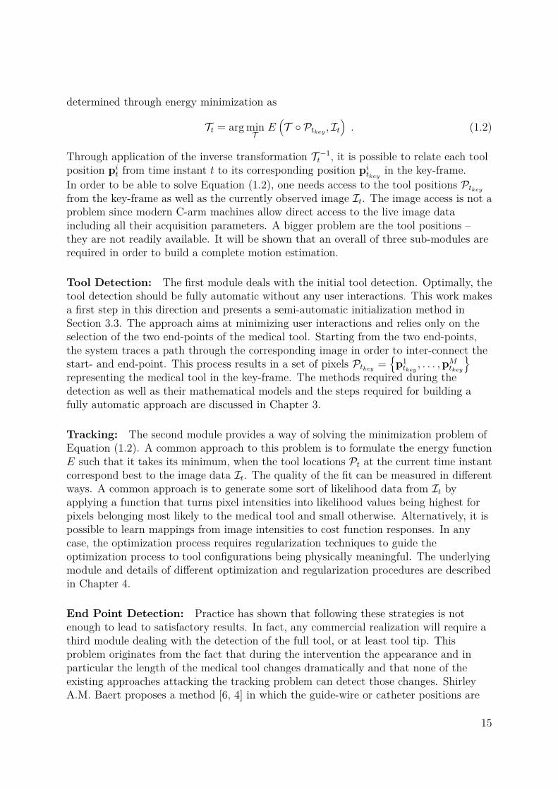
determined through energy minimization as

Tt = arg minT

E(T Ptkey , It

). (1.2)

Through application of the inverse transformation T −1t , it is possible to relate each tool

position pit from time instant t to its corresponding position pitkey in the key-frame.In order to be able to solve Equation (1.2), one needs access to the tool positions Ptkeyfrom the key-frame as well as the currently observed image It. The image access is not aproblem since modern C-arm machines allow direct access to the live image dataincluding all their acquisition parameters. A bigger problem are the tool positions –they are not readily available. It will be shown that an overall of three sub-modules arerequired in order to build a complete motion estimation.

Tool Detection: The first module deals with the initial tool detection. Optimally, thetool detection should be fully automatic without any user interactions. This work makesa first step in this direction and presents a semi-automatic initialization method inSection 3.3. The approach aims at minimizing user interactions and relies only on theselection of the two end-points of the medical tool. Starting from the two end-points,the system traces a path through the corresponding image in order to inter-connect thestart- and end-point. This process results in a set of pixels Ptkey =

p1tkey

, . . . ,pMtkey

representing the medical tool in the key-frame. The methods required during thedetection as well as their mathematical models and the steps required for building afully automatic approach are discussed in Chapter 3.

Tracking: The second module provides a way of solving the minimization problem ofEquation (1.2). A common approach to this problem is to formulate the energy functionE such that it takes its minimum, when the tool locations Pt at the current time instantcorrespond best to the image data It. The quality of the fit can be measured in differentways. A common approach is to generate some sort of likelihood data from It byapplying a function that turns pixel intensities into likelihood values being highest forpixels belonging most likely to the medical tool and small otherwise. Alternatively, it ispossible to learn mappings from image intensities to cost function responses. In anycase, the optimization process requires regularization techniques to guide theoptimization process to tool configurations being physically meaningful. The underlyingmodule and details of different optimization and regularization procedures are describedin Chapter 4.

End Point Detection: Practice has shown that following these strategies is notenough to lead to satisfactory results. In fact, any commercial realization will require athird module dealing with the detection of the full tool, or at least tool tip. Thisproblem originates from the fact that during the intervention the appearance and inparticular the length of the medical tool changes dramatically and that none of theexisting approaches attacking the tracking problem can detect those changes. ShirleyA.M. Baert proposes a method [6, 4] in which the guide-wire or catheter positions are

15

iteratively refined. The tool length is increased in tangential direction until the endpointis advanced beyond the endpoint of the guide-wire or catheter.

16

Together, the three modules described above build the motion compensation module.Applying a two-step procedure of tracking and tool extension after the system isinitialized results in the desired transformation Tt which allows the system to detect andtransform tool positions computed at time instant t to the key-frame and from there tothe pre-interventionally computed DSA. In applications, where an overlay of the DSAwith the current fluoroscopic view is required, the computed transformation could beused to transform the DSA image. This allows a blending in which the apparent motionwould be compensated.

17

CHAPTER

TWO

PREVIOUS WORK

Chapter two covers previous research performed in different areas which are relevant tothis thesis. In Section 2.1 methods on enhancement of tubular structures are discussedand summarized. These are of particular importance, because they are directly affectingall components required in the detection and tracking pipeline. The next part,Section 2.2 provides an overview of work related to the detection of medical tools.Finally, the recently growing interest of work in the field of tracking is covered inSection 2.3.

2.1 Enhancement of Tubular StructuresTubular structures are elongated line-like structures appearing at a specific width. Theseobjects are also referred to as curvilinear structures which are important for a multitudeof applications. In aerial images e.g., roads, railroads and rivers appear as curvilinearstructures. Other examples come from medical imaging. Here, tubular structures appearoftentimes in angiograms, where vessels are visualized in 2D or 3D. In ophthalmologyfundus images are of special interest because they contain indications about diseases ofthe eye and the primary diagnosis indicator are changes and abnormalities ofvascularization. Performing measurements on vascularization is based on techniques forthe analysis of tubular structures. Of most importance for this thesis is the enhancementof medical tools and in particular the enhancement of needles, guide-wires and catheters.Because the enhancement of tubular structures is of such importance in variousapplications the topic received a considerable amount of interest in the past. The mainfocus of this section are mathematical methods for enhancing the visibility of curvilinearstructures. Such an enhancement is a common pre-processing step for segmentationmethods and the enhancement can be performed such that the output image intensitiescan be interpreted as likelihood values. In such images high intensities correspond topixels having a high probability of belonging to a line-like structure and low intensitiesrepresent background pixels. Oftentimes, methods for extracting centerlines [44] oftubular structures have some overlap with those enhancing the structures. For this

19

thesis image processing methods enhancing those structures are of primary interest andthose are the methods which are revisited in this section.In his work on “Finding Edges and Lines in Images” [14], Canny discussed not only edgedetection methods but also the enhancement of ridges and valleys. When interpretingimages as height fields, where the intensity value of a pixel corresponds to a heightvalue, curvilinear structures appear in this landscape of image intensities either asmountain ridges or a valleys. According to Canny, “the only reason for using a ridgedetector is that there are ridges in images that are too small to be dealt with effectivelyby the narrowest edge operator”. The scenario he is referring to is exactly what can beobserved for medical tools since they appear only as tiny and thin structures within themedical images. Canny furthermore observed, that accurate estimates of ridge directionsare much harder to obtain than edge-directions. He states that the principal curvature,while being normal to the ridge direction, is a much less reliable quantity to measurefrom even in smoothed images. As a consequence Canny concludes that the detection orenhancement of curvilinear structures requires several oriented filer masks at each point.Since this early work, several strategies for the enhancement of ridges (or valleys) havebeen investigated.Koller et al. [39] propose to combine first and second order image filters for theenhancement of ridges. The authors build a line enhancement function by using the firstderivative of a Gaussian G′σ(x) which is a well known edge detector [13]. Given a brightbar profile of width w which serves as an approximation of an intensity ridge, theGaussian derivative G′σ(x) enhances the ridge edges on the left- and right-hand side ofthe profile. Following this observation, one can create shifted filters El = G′σ(x− w

2 ) andEr = −G′σ(x+ w

2 ) which, when convolved with the image, detect the left and rightprofile edges at x = 0. The authors combine the convolution responses in a non-linearway to overcome multiple line responses and sensitivity to edges, and the finalone-dimensional filter becomes

R(x) = min (pos(El ∗ f(x)), pos(Er ∗ f(x))) . (2.1)

Switching from bright (ridges) to dark (valleys) profiles, affects the shifted filters in theirsign and the function pos(x) maps all negative values of x to zero and acts as an identifyoperator on all other values. In 2D, the filter slightly changes because only the gradientsorthogonal to the ridges must be evaluated. To achieve this, the responses of the filtersEl and Er have to be projected on the ridge-normals which are the directions of principalcurvature of the ridge. These direction correspond to an eigenvector of the Hessian ofimage intensities in each pixel which is covered in more detail in Section 3.2. Anothertopic which will be covered in this section is the choice of the smoothing parameter σ.A different approach is proposed by Palti-Wasserman et al. in [58]. They suggest to usea modified Laplacian as well as a modified Marr-Hildreth [36] operator in order toenhance guide-wires while reducing the influence of noise. The authors achieve thisbehavior by adapting the original filters such that they act more globally. Each point iscompared not to its immediate 8-neighborhood (in case of 2D data), but to more distantpoints in the image. The optimal filter size is depending on the width of the guide-wirethough the authors suggest an empirical value of 11 pixels. In addition to modifying the

20

filters, the method is based on a fuzzy zero-crossing detection. The detection method isfuzzy in the sense that a pixel is marked as a zero crossing as soon as it has an intensityvalue smaller or equal than a specific threshold. The authors’ second filter, the modifiedMarr-Hildreth filter is a smoothed version of the modified Laplacian. It requires anadditional parameter in order to control the amount of smoothing.Frangi et al. [22] proposed another measure, which is based on the eigenvalues of theHessian matrix. The Hessian matrix H describes the second-order structure of localintensity variations around points of an image. The eigenvalues of H correspond to theprincipal curvatures and for line-like structures the eigenvector corresponding to thesmallest absolute eigenvalue points along the vessel. The approach is an extension of theworks of Sato et al. [66] and Lorenz at al. [50] who also use the eigenvalues of theHessian to locally determine the likelihood that a vessel is present. Frangi et al.modified these works by considering all eigenvalues and by giving the vesselness (orline-likeliness) measure an intuitive, geometric interpretation. Their measure consists ofthree components in 3D and two in 2D respectively. Assuming sorted eigenvalues|λ1| ≤ |λ2| ≤ |λ3|, the 3D specific component is based on the ratio of the largest absoluteeigenvalues

RA = |λ2||λ3|

. (2.2)

The measure is used to distinguish between plate-like and line-like structures and will bezero for the latter. The second component applies to the 2D and 3D case and measuresthe deviation of the observed structure from a blob-like or circular structure. It iscomputed as

RB = |λ1|√|λ2λ3|

. (2.3)

A last component is used to evaluate the amount of information contained in the Hessianby computing the Frobenius norm of H. For a real and symmetric matrix, the measure iscomputed as S =

√∑λ2i . This value will be low in background areas where no structure

is present and it becomes larger in areas of high contrast. The final filter response isbuilt up by combining the values through Gaussian distributions resulting in a scalarfilter response which can directly be interpreted as a likelihood value. The problem thisfilter poses for the user is the choice of three parameters (two in the 2D case) for theGaussians. Further details of the choice of these parameters are discussed in Section 3.2.

2.1.1 Scale-Space TheoryThese days, most of the research dealing with the detection or enhancement ofcurvilinear structures in 2D or 3D utilizes in some way differential geometry. Of specialinterest is the Hessian matrix (here exemplary for the 2D case)

H =[Ixx IxyIxy Iyy

](2.4)

21

which describes the second order structure of intensities of an image I. A first problemis that the computation of the Hessian requires second-order differentiation of the imageintensities and this differentiation process is ill-posed. The problem is ill-posed becauseof noise introduced by the acquisition process which is unavoidable. Consequently,differentiation of images requires regularization and a detailed analysis of thisobservation has been presented by Torre and Poggio [74]. The authors conclude, thatGaussian derivative filters are nearly optimal filters for computing image derivatives. Aproblem that arises in this context is how to choose the parameter σ – the scale – of theGaussian.Where is now the connection between scale-space and the enhancement or detection ofline-like structures? An intuitive idea, of why different scales are required here isbecause line-like objects are viewed from different distances or have different physicalsizes. Both cases result in the images of the objects to be of different size. Hence, thedetection of tubular objects requires a way to define the scale, i.e. the size of theline-like structure in the image. This scale is typically unknown and Witkin [82]proposed to obtain a multi-scale representation of the image. This multi-scalerepresentation is generated by the convolution of the image with different Gaussianfilters, where the parameter σ defines the scale. This pencil of filtering functions andtheir responses define the scale-space.When performing analysis in scale-space, in particular when trying to select “optimal”scales, additional modifications are required. Lindeberg [47, 48] analyzed the problem ofoptimal scale selection and introduced so called γ-normalized filters. In Lindeberg’sframework a one-dimensional γ-normalized Gaussian filter is written as

tγ/2 1√2πt

exp(−x2

2t

). (2.5)

Here, the parameter t = σ2 is referred to as the scale space parameter. Thenormalization constant γ is used, to ensure that a Gaussian based filter response yieldsonly a single maximum within a potentially limited scale support. In some scenarios,the parameter can also be used to modify the response function’s shape such that themaximum is reached exactly at a specific scale. Specific examples and mathematicaldetails will be presented in Section 3.1.

2.2 Detection of Guide-Wires and NeedlesTracking algorithms estimate the motion of an object between two points in time. Givenan object location at time ti−1, the algorithms estimate the position of the same objectat another point int time ti. When such an algorithm is initially executed, the spatialinformation at some time t0 is needed. This phase, when no a priori knowledge isavailable is oftentimes referred to as the initialization phase. During this phase, someway is required to detect the object, i.e. to determine its initial position in space. In thescenario of medical tool tracking, this means to be able to detect the object in the imageonly based on limited constraints regarding its position. Due to the limited constraints,this problem is much more difficult than the actual tracking step.

22

If a fully automatic method existed to solve this problem without a priori knowledge,tracking and other post-processing steps would not be required anymore. Unfortunately,the problem is so ill-posed, that currently no fully automatic methods exist whichperform this task so reliably, that it could be applied in clinical practice. But why is theproblem ill-posed? And why is the problem at all underlying any constraints? Thereasons for the problem to be ill-posed are manifold. The list below gives a briefoverview of some of the reasons:

• Multiple Tools: A first problem is that during minimal invasive proceduresoftentimes multiple tools are used. Using for instance several catheters is notuncommon during cardiac interventions. All of them might be visible and withoutany user interaction it is not clear, which of these tools is the object of interest. Apossible approach to handle such a situation is to use all potential candidates.This, however, would lead not only to a more complicated tracking algorithm butalso to reduced performance regarding the run-time. Considering the fact, that thetracking is only one of many components required for a navigation application, itis important to minimize computational requirements.

• Background Clutter: For a human observer, background clutter is usually not aproblem. This is especially then true, when observing dynamic scenes like forinstance a video stream as it is the case during fluoroscopy guided interventions.For a computer on the other hand side the situation is different. In fluoroscopicimages, anatomical structures like bone-tissue interfaces can have a quite similarappearance as guide-wires or needles. Therefore, background clutter ultimatelycauses similar problems as Multiple Tools do. The initialization algorithm requiresguidance to be able to select the correct tool of interest.

• Noise: The detection process is usually based on an early preprocessing stage inwhich candidate pixels potentially belonging to tools are highlighted. As has beendiscussed before in Section 2.1 many methods for the enhancement of tubularstructures rely on second-order image filters. These filters get unstable in thepresence of noise which was also discussed by Canny [14] and generate spuriousresponses when the SNR is low. Additional feature responses created due to noiseare more difficult to deal with than those created by multiple tools. Simply addingall false positive responses to the tracking algorithm does not only increase therun-time but it also leads to noise in the motion estimation. This is the casebecause noisy background cannot be assumed to exhibit motion which is free ofnoise.

• Tool Size: Guide-wires and interventional needles have small diameters resultingin bad visibility within fluoroscopic sequences. The physical diameters ofguide-wires are typically in the range of 0.5 to 1.0 mm and a common biopsyneedle size is 14-gauge (i.e. 2.108 mm). The resulting projections are often justaround pixel wide and even result in multiple disconnected lines. This hasimplications on image filtering techniques because scale-space filter responses orfor many methods designed such that they take their optimal response at a scale

23

that corresponds to the ridge radius, i.e. half the tool diameter and thus the scalecan be as 0.5 pixels. When using such small scale values for image filtering, theinfluence of discretization effects is strongly degrading the responses and results innoisy responses.

• Temporal Averaging: In order to improve image quality hardware-vendors ofmedical imaging devices such as C-arms integrate signal processing algorithms intheir machines. One common method to reduce the speckle-noise observed inlow-dose X-ray videos is the use of temporal averaging. A straight forwardapproach of this methods takes a number of images in a fixed size time-windowand computes the average of these images. Indeed, this method reduces thespeckle-noise but is not without drawbacks. The main problem behind thismethod is that in dynamic scenes with apparent motion, temporal averaging willcause phantom responses of objects resulting from different spatial locations ofthese objects. Such phantom locations are disturbing detection systems becauseagain, it is not clear which responses are the correct ones belonging to the actualtool position.

All these issues make the detection task a difficult problem. The remainder of thissection gives a brief overview of how researchers tried to solve the aforementioned issuesor at least how to reduce their influence. The approaches are quite different rangingfrom semi-automatic methods to attempts at fully-automatic procedures.Palti-Wassermann et al. [58] propose to use a semi-automatic method for the detectionof guide-wires which is based on fitting second-degree polynomials in “limited activewindows”. Initially, the authors pre-process the input image with modified Laplacian orMarr-Hildreth filters. The filters are modified such that they enhance intensity ridgesinstead of corners. This is achieved by altering the influence range of the original filtersin combination with an adapted method for the labeling of zero crossings. A fuzzylabeling process of zero-crossings allows to turn the image into a binary form where onlypotential ridge pixels are colored white and all other pixels are marked as black. In anext step, the authors approximate the guide-wire shaped by a second-degreepolynomial y = ax2 + bc+ c. To calculate the parameters a, b and c, three pointsbelonging to the guide-wire need to be known. This requirement can be reduced byassuming two points, e.g. the end-points of the guide-wire are provided by the user.Once this condition is met, guide-wire locations can be represented by a singleparameter and the authors chose to use b as their unknown variable. The parameterestimation is performed in sub-windows along the curve by applying a Houghtransformation to the local window. After this transformation, the parameter bcorresponding to the guide-wire is selected as the value corresponding to the maximumof the histogram of b-values in the sub-window. Given this parameter, the second-orderpolynomial representing the guide-wire part passing through the sub-window iscompletely known. In a next step, the sub-window is advanced further along the curveand starting from the known two overlap points, the procedure is applied iterativelyuntil the local window is finally placed on the guide-wire’s end point. The authors usefurther techniques such as dynamic histogram size, b-value thresholding and

24

pixel-grouping to enhance the detection method. Regarding future work, the authorsargue that “time must be added” to increase the level of automation.Carsten Steger developed a robust and fast method in his research on the detection ofcurvilinear structures [70, 71]. The method results in multiple sets of points, where eachset represents one line. Multiple properties are assigned to each point. The propertiesinclude the point’s sub-pixel location, the line normal, line width, its strength and itstype (end-point, center-point or junction-point). The algorithms starts by computingthe line’s normal directions for each point. This is done in the same way as during theenhancement of tubular structures. The direction (nx, ny) is computed as theeigenvector of the Hessian of image intensities which corresponds to the eigenvalue ofmaximum absolute value. In a next step, the point’s sub-pixel location is computed byinserting (dx, dy) = (t nx, t ny) into the Taylor polynomial

I(x+ dx, y + dy) = I(x, y) + (dx, dy)(IxIy

)+ 1

2(dx, dy)(Ixx IxyIxy Iyy

)(dxdy

)(2.6)

and setting the derivative along t to zero. It turns out, t can be compactly representedas a function of the line normal and first- and second-order derivatives. To ensure, thatthe final pixel location is within the unit-circle centered at (x, y), only points witht ∈

[−1

2 ; 12

]are accepted as line points. This first step results in a sub-set of the initial

image pixels and associated sub-pixel locations (x+ dx, y + dy).In a next step, pixels are linked together to form line segments. The system stores foreach pixel, its sub-pixel location, its direction and its ridge strength. These values arethen used to perform the actual linking. First, depending on the edge direction, thethree candidate neighbors are selected for each pixel. This procedure is depicted inFigure 3.12. From the potential neighbors, the one that minimizes d+ c β is chosen.Here, d = ‖p1 − p2‖2 is the euclidean distance between two sub-pixel points andβ = |α1 − α2| ∈ [0, π/2], is the angle difference between the two points. In his work,Carsten Steger used c = 1 throughout his experiments. Similar to hysteresisthresholding, the linking process is controlled by two thresholds. A first, high thresholdis used to determine whether a new line segment is created. As long, as the systemdetects a pixel with a second directional derivative being bigger or equal to the highthreshold. A second, lower threshold is used to determine when the tracing of a linesegment is terminated. In case all potential neighbors have second directional derivativebeing lower than the second threshold, the current line segment tracing is stopped. Theedges and the width of line segments are determined similarly to what has been done forthe sub-pixel locations. The paper proposes additional methods in order to deal withlines that having asymmetrical profiles. The evaluation has been primarily performed onaerial images though the work also contains examples from a coronary angiogram. Oncecorrect parameters are chosen, the method is fully automatic. As it is often the case,good parameters can be estimated from properties of the expected line profiles. Theproblem on the other-hand side is that the method is detecting many points andsegments resulting from background clutter. Currently, the correct lines must be chosenmanually, or it must be accepted that only parts of the medical tools are extractedfully-automatically. Similar to the previous approach, a stable fully-automatic system

25

needs to incorporate time information during the detection process.The algorithm presented by Can et al. [11] focuses on vessel segmentation in fundusimages. The authors propose a tracing algorithm which works recursively given a set ofinitial seed points. Seed points are detected by sampling the image along a grid ofone-pixel-wide lines and by detecting local gray-level minima along these lines. Thisapproach will choose points lying most probably on vessels which appear as dark tubularstructures in fundus images. Once the seed points p0 are computed, the algorithmcontinues by recursively adding new neighbors pk to the seeds. Here, k is representingthe time-step or iteration. Vessel directions sk are discretized into 16 fixed orientations,one every 22.5. To determine the direction sk for a point pk, directional filters areapplied on the left- and right-hand side of the vessel, orthogonal to the currently probeddirection s. These filters are not only applied for different potential orientations s butalso at different distances to the current centerline location pk. The left- and right-handside filter searches result in responses Rmax(s) and Lmax(s). The optimal orientation ischosen as 1

sk+1 = arg maxs

(max (Rmax(s), Lmax(s))

)(2.7)

and the tracing follows the strongest ridge by setting the new position vectorpk+1 = pk + αuk+1. The vector uk+1 corresponds here to the unit vector pointing in thedirection defined by sk+1. The iterative procedure is stopped when a new point pk+1 islocated outside the image or when a previously detect vessel intersects the current one,or when the sum of the filter responses falls below a certain threshold T ,|Rmax(sk+1) + Lmax(sk+1)| < T . Additionally, the authors took care in their method todevelop approaches to extract branching and cross-over points while aiming at a highlevel of automation and robustness. To summarize, the method proposed by Can et al.uses vessel tracing which does not require global image filtering but only local filterapplication. The method is capable of extracting the whole vessel tree from fundusimages while offering good performance both in terms of robustness and run-time.Nonetheless, the method can not be seen as a fully automatic implementation for vesselor tool detection. The robustness is depending on the choice of several parameters suchas grid size, neighborhood size, and amongst others the step size used to select the nextneighbor. Despite the parameter choice, the algorithm is potentially detecting orsegmenting more candidates as are of interest for the application of guide-wire tracking.No improvement has yet been made on detecting and removing false positivesegmentation results.Another algorithm based on tracing vessels is proposed by Schneider et al. [67]. Theauthors use a Hessian based algorithm for the segmentation of vessels. The method isgeneric and can also be applied to the detection of medical tools such as guide-wires orneedles. The idea is based on using not only the eigenvalues of the Hessian matrix ofimage intensities but also the eigenvectors as well as a likelihood image (e.g. Frangi’s[22] vesselness). Given initial seed points, the algorithm propagates a wave front in thedirection of the eigenvector corresponding to the smallest absolute eigenvalue. The

1The formula has been slightly rewritten. Its orignal can be found in [11], in Equation (7).

26

segmentation result keeps growing iteratively until the following boolean criteria isfulfilled: (∣∣∣v>1 v′1

∣∣∣ ≤ θα)∨((V < θV ) ∧ (λ1 ≥ θλ1 ∨ λ2 ≤ θλ2)

)(2.8)

The first term is corresponding to a smoothness criterion and ensures that neighboringpoints exhibit similar directions. The second, two-component term ensures, that eitherthe likelihood of the currently selected point is high enough, or that the eigenvaluesexhibit characteristics corresponding to a bifurcation. The last term, the bifurcationcheck is required because it is common that eigenvalue based vesselness measures aredegraded on bifurcations. The authors coined the resulting vessel or tool representationas streamline representation and argue that it provides additional information about theglobal object shape. One example are length and density maps. The length mapassociates to each pixel the length of the longest fiber crossing its location. Similarly,the density maps represents for each pixel a counter of how many fibers passed throughits location. So far, the procedure does not result in a single pixel wide segmentationand thus rely on additional thinning techniques to create a representation of the centerline only. The thinning is performed by iteratively removing pixels that do not fulfillcertain criteria depending on the current pixel’s density and the expected object lengthand uniqueness. Finally, the authors propose a method that allows the detection ofcatheters and their removal from vessel images. The idea is based on heuristicsregarding the length of the catheter and its shape. The authors claim that catheterstypically pass through the whole image and “have a rather straight shape with smallconstant curvature”. The authors assess the curvature by fitting B-splines to streamlinecandidates and by computing curvature responses analytically on the estimated B-splinecurves. Angular changes and the segment length are then computed against empiricallyestimated values in order to classify a segment as being a guide-wire or not. Altogether,the method is promising but still requires user interactions. In case seed points weredetected automatically, one would be facing the same problem as before – segmentationresults from the anatomical background without obvious ways to detect or remove them.A different, learning-based approach for the detection of guide-wires has been proposedby Mazouer et al. [54]. As opposed to their previous work [7], the authors extended thenew method such that it allows user-interactions to constrain the detection process. Themethod allows to follow two distinct paths for the guide-wire detection. A first pathallows to perform a fully-automatic detection which can be refined by interactivelyadding additional constraints. The second path performs already the initial detectionbased on constraints provided by the user.The overall system consists of several modules. In the beginning constant lengthsegment candidates are extracted by a low-level segment detector. To each segmentthree parameters (x, y, θ) are associated, where (x, y) is the segment location andθ ∈ [−90; 90] the segment orientation. The segment detector is based on Haar featuresand uses a probabilistic boosting tree (PBT) for the detection process. The secondcomponent is a curve classifier, again based on a PBT. The curve classifier is used tomodel the shape and appearance of an n-segment curve. In the initial work by Barbu etal. [7], the probability of a guide-wire consisting of segments s1 to sn and end-points xB

27

and xE is computed as

P (G(s1, . . . , sn, xB, xE)) = P (C(s1, . . . , sn))PE(xB)PE(xE) . (2.9)

The guide-wire with the highest probability is reported as the final localization resultwhen the fully automatic procedure is being used. For the path that allows userinteractions, Mazour et al. introduced a novel scheme. So far, the method is based onsegments sk and probabilities P (si, sj) of connecting two segments. User inputs areprovided as two dimensional point coordinates (x, y) on the guide-wire. In order to benow able to incorporate these coordinates into the probability framework, probabilitiesof connecting a given point with already known segments is required. Theseprobabilities are computed based on a so called extension field (EF) introduced by Guyet al. [30]. Once the missing probabilities are available, dynamic programming (DP) isused to connect the segments as well as the user inputs.In their evaluation the authors report false detection rates of below 5% as soon as fiveuser interactively selected points are available. Given the same number of userinteraction, the missed detection rate reaches similar values. As an average annotationtime for full guide-wires including loops the paper reports about 6.23 seconds.The methods above represent more than 10 years of research and constitute only afraction of what has been done in the field of ridge detection. The applications arevarious ranging from aerial image analysis over the detection of vasculature to thedetection of medical tools. The approaches range from early image processing and imagefiltering techniques over approached using ridge tracing to learning based methodsincluding hybrid solutions which aim at utilizing the benefits from all worlds. There isstill a trend towards semi-automatic methods that allow user interactions because formany applications the fully-automatic approaches do not yet meet the strong real-worldrequirements. In particular the robustness, i.e. being able to distinguish spuriousline-like structures from the desired objects is often-times difficult. Since so far, allmethods are based on static images, future work is probably going to investigate theintegration of temporal information which might give additional clues about how todetect and remove noisy image structures.

2.3 Tracking of Guide-Wires and NeedlesIn this section existing approaches are discussed which mainly deal with the problem oftracking guide-wires during fluoroscopic interventions. The problem is yet unsolved andin no commercially available system integrated. First publications working on the ideaof enhancing navigation during fluoroscopic interventions appeared in the mid 80s – thatmeans we are already looking back at a quarter century of research. Since then, avariety of work has been performed in the direction of navigation aids and on theenhancement and detection of medical tools. Surprisingly, image-based (deformable)tracking of medical tools has only relative recently received growing interest and itseems as if it still keeps growing.Baert et al. [5, 3] propose a guide-wire tracking procedure based on energy minimizationof a B-spline parameterization. The method is stratified, i.e. the motion estimation is

28

performed in two steps. At first a rigid transformation of the guide-wire is estimatedwhich is followed by computing the remaining deformable component.The rigid transformation, here translation only, is determined by creating a binarytemplate from the currently known guide-wire positions. Once the template is given, theoptimal location in the new frame is determined by maximizing the template’s crosscorrelation within a certain search region in the new image. The cross correlation can becomputed on the original image intensities or some feature image highlighting line-likestructures.The deformable motion component is estimated by energy minimization using Powell’sdirection set method. To this end, the guide-wire shape is approximated by athird-degree B-spline curve defined as

C(u) =p∑i=0

Ni,3(u)Pi , 0 ≤ u ≤ 1 . (2.10)

In the papers of Baert et al. [5, 3, 4] 3 or 4 control points were used to model differentguide-wire shapes. The optimization is now carried out, by finding displacements di foreach control point Pi such that the displaced curve corresponds in an optimal way to thecurrent fluoroscopic frame. Because mere image based constraints lead to an ill-posedformulation, the deformed curve must adhere to additional geometric constraints. Theoptimization is formulated as an energy minimization and the energy function modelsthe aforementioned components by external and internal forces.The external forces are based on feature images F . These are constructed by enhancingline-like structures with and without using directional information of the initial splineposition. The structures are enhanced in unprocessed images, in background-subtractedimages as well as in images which are preprocessed by coherence enhancing diffusion(CED). As the internal energy the authors have chosen to penalize the curvature κ ofthe curve at a given point. The overall energy is formulated as

E =n∑i=0

(ακ2(i) + F (i)

)l(i) . (2.11)

Here, n = 100 is the number of samples used along the spline curve. The weightingparameter α = 6.25 is used to control the influence of the internal energy. F (i) and κ(i)are the values of the external and internal energy for the i-th sample point on the curveand l(i) can be interpreted as the integration step.For this work it is of most interest to note that the authors conclude that Hessian featureimages allow to achieve results with a precision “similar to the inter-observer variability”.This indicates that it is not essential to use advanced preprocessing methods such asCED which is advantageous because such methods would lead to longer processingtimes. The authors report running-times of about 5 seconds per frame and suppose thata reduction by an order of magnitude is possible after optimizing the method.Slabaugh et al. [69] present a similar approach. The authors are also using a stratifiedapproach, i.e. perform a rigid as well as a deformable registration and they are alsomodeling guide-wires as B-splines. Besides these similarities, the work presents variousnovelties. As before, the curve locations are determined by energy minimization. Here,

29

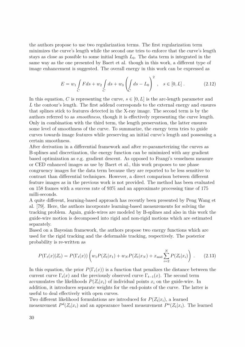
the authors propose to use two regularization terms. The first regularization termminimizes the curve’s length while the second one tries to enforce that the curve’s lengthstays as close as possible to some initial length L0. The data term is integrated in thesame way as the one presented by Baert et al. though in this work, a different type ofimage enhancement is suggested. The overall energy in this work can be expressed as

E = w1

∫C

Fds+ w2

∫C

ds+ w3

∫C

ds− L0

2

, s ∈ [0, L] . (2.12)

In this equation, C is representing the curve, s ∈ [0, L] is the arc-length parameter andL the contour’s length. The first addend corresponds to the external energy and ensuresthat splines stick to features detected in the X-ray image. The second term is by theauthors referred to as smoothness, though it is effectively representing the curve length.Only in combination with the third term, the length preservation, the latter ensuressome level of smoothness of the curve. To summarize, the energy term tries to guidecurves towards image features while preserving an initial curve’s length and possessing acertain smoothness.After derivation in a differential framework and after re-parameterizing the curves asB-splines and discretization, the energy function can be minimized with any gradientbased optimization as e.g. gradient descent. As opposed to Frangi’s vesselness measureor CED enhanced images as use by Baert et al., this work proposes to use phasecongruency images for the data term because they are reported to be less sensitive tocontrast than differential techniques. However, a direct comparison between differentfeature images as in the previous work is not provided. The method has been evaluatedon 158 frames with a success rate of 93% and an approximate processing time of 175milli-seconds.A quite different, learning-based approach has recently been presented by Peng Wang etal. [79]. Here, the authors incorporate learning-based measurements for solving thetracking problem. Again, guide-wires are modeled by B-splines and also in this work theguide-wire motion is decomposed into rigid and non-rigid motions which are estimatedseparately.Based on a Bayesian framework, the authors propose two energy functions which areused for the rigid tracking and the deformable tracking, respectively. The posteriorprobability is re-written as

P (Γt(x)|Zt) = P (Γt(x))(w1P (Zt|x1) + wNP (Zt|xN) + xmid

N∑i=2

P (Zt|xi))

. (2.13)

In this equation, the prior P (Γt(x)) is a function that penalizes the distance between thecurrent curve Γt(x) and the previously observed curve Γt−1(x). The second termaccumulates the likelihoods P (Zt|xi) of individual points xi on the guide-wire. Inaddition, it introduces separate weights for the end-points of the curve. The latter isuseful to deal effectively with open curves.Two different likelihood formulations are introduced for P (Zt|xi), a learnedmeasurement P d(Zt|xi) and an appearance based measurement P a(Zt|xi). The learned

30

measurement is computed from the numerical output f(z, xi) of an AdaBoost classifierfor any given point xi. It takes its maximum, when the classification value of f(z, xi) ismaximal. The AdaBoost classifier is trained with a set of offline collected data.Appearance based measurements are evaluated by the likelihood P a(Zt|xi). Here, thelikelihood becomes maximal, when the image patch centered at xi in the current frameis most similar to the patch centered at the corresponding location in the previous (oralternatively initial) frame. The general likelihood term is computed as

P (Zt|xi) = P d(Zt|xi)P d + P a(Zt|xi)P a , (2.14)

where P d and P a are priors for the two types of measurement models. Wang et al.propose so called kernel-base measurement smoothing for the likelihood functions. Thisadditional modification allows them to perform a hierarchical and multi-resolutiontracking and the details can be found in [79].During the solution of the rigid-tracking, the authors maximize the posteriori based onEquations (2.13) and (2.14). This is not the case during the estimation of thedeformable component. In the latter case, additional terms for the regularization of theproblem are introduced. These terms are integrals of first- and second-order derivativesof guide-wire curves, and act as guide-wire smoothness priors.The algorithm has been evaluated on 47 clinical sequences. It achieves an overallguide-wire tracking precision of 1.8 pixels and is currently processing data at 2 framesper second (i.e. 500 ms per frame). The authors claim that near real-time speed can beachieved with an optimized implementation based on multi-threading and GPUaccelerations. Learning appearance models or likely deformations of guide-wires seemslike a promising direction though currently they impose the additional difficulty to meetrequired real-time constraints.

Table 2.1: Overview of different guide-wire tracking methods.method parameter

estimationlikelihood prior stratified fps a

Baert [3] continuous feature image (Hessian,CED, . . .)

curvature X 0.2

Slabaugh [69] continuous feature image (phasecongruency based)

curvature &length changes

X 5.7

Wang [79] coarse-to-fine,exhaustive

AdaBoost classifier &intensity differences

displacements& derivativenorms

X 2

Method A discrete feature image (Hessian &gradient based)

length changes – 20

Method B discrete SVR of orthogonal intensityprofiles

length changes – 1.5

a The given run-times cannot directly be compared since they are assessed on different systems.They serve mainly to get an idea of the magnitude of the algorithm run-times.

To summarize, all methods dealing with guide-wire tracking are using B-splines formodeling curvilinear medical tools (guide-wires, catheters and even needles since they

31

may bend). Furthermore, it is important that the methods presented in this work aswell as the aforementioned methods are tracking a segment of a medical tool whiletrying to prevent that this segment is vanishing. This implies, that all methods mayrequire an additional procedure to perform the full tool detection or at least the tool-tipdetection. A possible approach of dealing with this end-point detection is presented byBaert et al. [6].The most important differences between the individual methods are summarized inTable 2.1. Here, the parameter estimation column is intended to provide a roughclassification of the underlying optimization process. Entries of the likelihood (externalenergy, data term) column are meant to be read as “is based on” or as “is a function of”and the entries of the prior (internal energy, regularization) column list whichgeometrical properties the authors are minimizing in order to constrain the set ofpossible solutions. Some approaches (so called stratified ones) decompose the probleminto a rigid and a non-rigid motion and solve both problems individually whereas othersrepresent the whole curve motion by a single displacement field – the second last columnstratified denotes to which of these two groups the method belongs. The last entry ofthe table is intended to give the reader a rough idea of the magnitude of the individualalgorithm’s run-times. Since the experiments were performed on separate systems withdifferent processors and program environments, these values cannot be directlycompared. Furthermore, the different methods offer different levels of potentialregarding optimizations which follows that faster run-times may be achieved.The key innovations of the method presented in this work can be summarized as follows.The algorithm introduced here is using discrete optimization to solve the parameterestimation. Discrete optimization has the advantage of being able to provide optimalsolutions within the discretized parameter space. This property reduces the likelihood ofthe optimization process to get stuck in local minima.Method A introduces a novel motion model and an adapted regularization scheme.Related tracking algorithms try to minimize geometric properties as e.g. curvature orthe first- and second-order derivative norms of the curve in order to impose smoothnesson the resulting curves and in order to prevent over-deformation. Slabaugh et al. [69]started to leave this path by penalizing absolute length changes, thus enforcing somelevel of self-similarity between the tracked curves and the curves as they are appearingduring the initialization. This work is adapting this regularization approach andintroducing a novel deformation model which is required to properly address discreteoptimization inherent approximation errors.A second learning based algorithm is briefly introduced in Section 6.2 and referred to asMethod B. The idea is to learn a mapping between orthogonal intensity profiles of curvesand the associated likelihood of belonging to a medical tool. This has the advantage ofbeing able to adapt to the tool appearance which is typical for fluoroscopic imagesequences including the influence of noise. Another advantage is that by learning anappearance model, one overcomes the problems which are inherent to image filteringbecause the learning can be performed on the raw and unprocessed image data.

32

CHAPTER

THREE

TOOL DETECTION

3.1 Modeling Tubular ToolsTubular tools, or those that appear as tubular or line-like after projection by an X-raysystem are of critical importance during the development of a tracking system. In thischapter the mathematical properties of line-like structures are revised. Only, when amathematical model for line-like structures is given, it is possible to understand, analyzeand optimize enhancement, detection and tracking algorithms. Already the modeling isnot an easy task. The fact that till today, researchers have no common agreement upona single mathematical model is one indicator that supports this statement.

3.1.1 X-ray AttenuationThe way in which tubular objects appear in images depends on various factors.Primarily, the appearance is defined by the physical rules underlying the imagingprocess of conventional X-ray. On a modern C-arm system, two-dimensional radiographsare acquired by an X-ray source and a planar, flat-panel detector. Image intensities aredepending on the amount by which X-rays are attenuated while passing through thebody. The attenuation of X-rays passing through a single object is an exponentialfunction which depends on the object’s attenuation coefficient. X-rays passing throughan object with a diameter d and with constant attenuation coefficient µ are measured onthe detector plane with an intensity of

I = I0 exp(−µd) . (3.1)

For objects with locally varying attenuation properties, this equation generalizes to

I = I0 exp(−∫µ(u)du

), (3.2)

where the parameter of the exponential term is the line integral through µ(u). In bothEquations (3.1) and (3.2), I0 is the intensity of the incident X-ray beam. Ideal X-raydetectors are producing images with intensities being proportional to the negative

33

x

y

α

r

l(cx, cy, r, α)

detector row

X-ray source S = (0, 0)>

C = (cx, cy)>

α

Figure 3.1: Idealized X-ray projection of a tubular object. The object is centered at C.The path lengths at which X-rays are attenuated in the tubular object vary with theprojection direction α. The path length is denoted as l(cx, cy, r, α) and two examples forα = 0 and α = 8 are shown in red.

logarithm of the attenuation intensities. An optimal projection image would have imageintensities corresponding to

I(x, y) = − log(I0) +∫µ(u)du . (3.3)

Image intensities are depending on the incident X-ray beam intensity I0, the attenuationcoefficients and the distance at which X-rays are traversing objects while beingattenuated. These observations allow the formulation and analysis of a simplifiedprojection model for tubular objects.

3.1.2 An Idealized Tube ModelFor the analysis of image intensities as generated by tubular objects, a simplified twodimensional projection model is considered. The setup is sketched in Figure 3.1. In thismodel, a coordinate system is centered in the X-ray source S. A single scan-line in theimage is generated by the attenuation responses measured on the detector row. Themeasurement are assumed to be corresponding to the ideal function of Equation (3.3).X-rays are emanating from the origin towards the detector row and the detectorexcitation is depending on the projection direction α. The model is parameterized suchthat for α = 0, the projection ray is passing through the center of a tubular structure.In Figure 3.1, this ray corresponds to the bottom ray.To be able to evaluate Equation (3.3), one needs to know for each projection direction αthe path length l at which the rays travel through the tubular structure. In this example,

34

the tubular structure is representing a cross-section of a three-dimensional object. For atwo-dimensional circular object C with a radius r, its equation is given implicitly by√

(cx − x)2 + (cy − y)2 = r . (3.4)

The general line equation of a projection ray lp deviating by the ray passing through theobject center at an angle α (e.g. the upper ray from Figure 3.1) can be written as

y = − sin(α)cx + cos(α)cycos(α)cx + sin(α)cy

x . (3.5)

If a projection ray lp and the object C intersect, two real-valued intersection points pinand pout can be computed from Equations (3.4) and (3.5). The length l as a function ofcx, cy, s and α, at which X-rays are traversing the circular object is then

l(cx, cy, r, α) = ‖pin − pout‖ (3.6)

= 2√r2 + (cos(α)2 − 1)(c2

x + c2y) . (3.7)

Combining now Equations (3.7) and (3.3) one can picture the synthetic intensity profilegenerated by a perfect C-arm system when imaging a tubular structure. Beforeassembling the final equation another simplification needs to be introduced. InEquation (3.3), the general case of varying attenuation along the X-ray path is assumedthough in this example the object C is assumed to have a constant attenuationcoefficient of µ. This assumption leads to the simplified equation 1

I(α) = − log(I0) + µl(cx, cy, r, α) (3.8)

= − log(I0) + 2µ√r2 + (cos(α)2 − 1)(c2

x + c2y) . (3.9)

The intensity profile from Equation (3.9) is not corresponding to reality for severalreasons – this is why it is referred to as idealized. The model depicted in Figure 3.1makes several strong assumptions which are not true in clinical practice. First, tubularobjects are in general not perfectly tubular; they are not even elliptic because manypatients undergoing procedures from interventional radiology have calcified vessels andsuffer from stenoses, aneurisms or other diseases of the vascular system. The secondreason why the model does not hold is because it assumes that the vessel is runningparallel to the detector plane. Again, this is not true because it can be arbitrarilyoriented with respect to the detector plane. This results in Equation (3.7) being only arough approximation which is typically underestimating the path length. The effect,which one observes in this case is foreshortening. A similar effect is caused by the fact,that the typical ray direction is not depending on a single angle α as in the givenexample. In order to describe a line direction passing through the origin, two angles forthe azimuth and elevation are required. There are more reasons, why the given model isnot general. They include background clutter, X-ray scattering, noise effects during theimage acquisition, just to name a few.

1The model and X-ray parameters are omitted for the sake of brevity.

35

−34π −

π2 −π

4 0 π4

π2

34π

0

5

10

15

I(α

)

µ = 1µ = 2µ = 4µ = 8

Figure 3.2: Idealized intensity responses of a tubular object with a radius r = 1 whichis located at a distance of 1 (i.e. c2

x + c2y = 1) to the X-ray source. The plot shows the

responses for a constant incident intensity of I0 = 1 for varying attenuation coefficientsµ. The functions correspond to the output of Equation (3.9).

The question may arise, why the modeling is then done this way if there are so manyreason rendering it inaccurate. One of the reasons is that incorporating all phenomenapresented before is close to impossible. Let us assume for a moment a simple formulawere available that modeled actual three-dimensional projection rays by incorporating asecond angle β. What would one gain in the analysis? In this section, our intention is togive a rough idea about the image generation process and how close different modelsproposed by different authors are to reality. It is not the intention to create a modelthat perfectly resembles reality.But there is more to ask since it could well be that a model which is closer to realitywould allow for a better modeling of the application. So again, let us assume weincorporated the second angle β. How could this help in a real application? There is noobvious way how that could help because in practice we have no a priori knowledgeregarding the vessel orientation within the patient. The orientation is even subject tochange during the intervention – one of the aspects this thesis tries to recover.To summarize, it is true, that the model is approximative but it is likewise as close toreality as it is useful for the following comparison. Some of the properties, like e.g. thelimited support of the function will not change when moving to more realistic models.In the next section, the curve model given by Equation (3.9) will be compared to modelsproposed by different authors.

3.1.3 Typical Tube ModelsDuring the analysis of enhancement filters which is following in the next section,mathematical models of contour intensities are required. This is especially then true,when the analysis is of analytical nature. Thus it is not a surprise, that already many

36

different models exists in the literature. It is also no more a surprise that there is not asingle model. The previous section has given some indications why the derivation of ageneric model is hardly possible.The different models which are used in today’s literature have different origins. Some ofthem are likely to be evidence based. The investigation of image data, be it of medicalnature or not, in combination with the knowledge about what is actually being imagesallows researchers to follow such a path. Other reasons may be that some models allowfor a simplified analytical investigation of model properties. Since in image processingthe convolution of image data with image filters is a fundamental procedure and becauseit has been already shown that especially for the analysis of edges and ridges Gaussianimage filters are most appropriate, having Gaussian image profiles is beneficial. This isthe case because in such a scenario, the convolution can easily be expressed analyticallyas it is just another Gaussian with a different mean and variance.A commonly used (e.g. [70, 71, 39]) model is the block model or bar shaped model.Besides its spatial location x, the model is only parameterized by a radius r and theridge height h. It can be defined as a piecewise function as

Ib(x, r, h) =

h, |x| ≤ r

0, |x| > r. (3.10)

An extension to this model has been proposed by Carsten Steger [71]. In his works onthe detection of curvilinear structures he wanted to be able to model different contrastlevels on the two ridge sides and thus introduced what he called the “asymmetrical barshape” model

Iab(x, r, a, h) =

0, x < −rh, |x| ≤ r

h a, x > r

. (3.11)

Another model of which we will show that it is most close to the previously derivedidealized model is a parabolic shape. As for the block model, it is only parameterized bythe object radius r and height h.

Ip(x, r, h) =

h(1− x2

r2

), |x| ≤ r

0, |x| > r. (3.12)

As opposed to the asymmetrical bar shape, the parabolic function in the form presentedhere, does not support different contrast levels on the two vessel sides. The last,commonly used model is a Gaussian model. Here, the radius is controlled by theGaussian’s variance, effectively controlling the radius of the function. A secondparameter is required to model the ridge height and it is incorporated as a simplescaling. Sato et al. [66] used a similar model in their work.

IG(x, σ, h) = h exp(− x2

2σ2 ) (3.13)

37

−2 0 20

1

2

Block Model

−2 0 20

1

2

Parabolic Model

−2 0 20

1

2

Gaussian Model

Figure 3.3: The figure shows optimal fits between three different ridge models and theidealized block model derived in Section 3.1.2. The models are (from left to right), a sym-metric block model, an elliptical model and a Gaussian model. The red curves representthe optimal models after fixing the width to the expected value while the green curvesshow the optimal models after fixing their height to the expected value.

What is of interest for the remainder of this work is how well each model canapproximate the idealized one. This question can be analyzed by finding for each modelI∗ the optimal parameters p such that the following quantity gets minimal

∞∫−∞

(I(x)− I∗(x,p)

)2dx . (3.14)

In order to be able to perform this derivation analytically, one of the parameters of eachmodel will be fixed (e.g. the radius r) and the remaining parameter p will be computedby solving

∂

∂p

∞∫−∞

(I(x)− I∗(x, p)

)2dx = 0 . (3.15)

The analysis has been carried out for the symmetrical profiles only. Including theadditional degree of freedom the asymmetrical bar profile is offering does not bring anyadvantages in terms of error reduction – for the block model, the minimal error that canbe achieved is identical to the asymmetrical bar shape. The three models that wereanalyzed are the block model (Equation (3.10)), the parabolic model (Equation (3.12))and the Gaussian model (Equation (3.13)).The function I(x) = 2

√cos(x)2 serves as a reference model. It is corresponding to the

idealized model response for a vessel at a 1 unit distance to the projection center, withincident intensity of I0 = 1 and a constant attenuation of µ = 1. For this function bothparameters are known, its exact radius r = π

2 and its height h = 2. The “optimal” modelparameters are determined by fixing one out of these two parameters. This approachdoes not necessarily reveal the global optimum of Equation (3.14) but it is most closelyrelated to the intended interpretation of the individual parameters and serves as anacceptable approximation.

38

For the block and parabolic model, both parameters can be easily fixed and theremaining parameter can be computed by solving Equation (3.15). Following thisapproach leads to analytical solutions for the optimal height parameters

hb = 4π

hp= 60π3 . (3.16)

The resulting curves corresponding to these parameters are the red curves in Figure 3.3.Because the Gaussian model has infinite support, it is not easily possible to fix themodel’s radius and thus the optimal height has not been computed in this case.Fixing the height in all three cases to h = 2 leads to a different set of curves and theseare corresponding to the green curves in Figure 3.3. Here, the optimal parameters couldonly be determined numerically and they resulted in

wb ≈ 1.04720 wp≈ 1.51513 σ ≈ 0.84173 . (3.17)

In Figure 3.3, the three optimal models are plot together with the reference function.Already a visual inspection of the three plots reveals, that the parabolic modelrepresents the most optimal fit. The block model is used primarily because of its simplemathematical properties but does not reflect well the physical properties. The Guassianmodel on the other-hand side results in a better approximation of physical propertiesbut again, it is primarily chosen because of its nice mathematical properties and inparticular its infinite support does not agree with reality.

3.2 Enhancement of Tubular StructuresIn this section several methods for the enhancement and detection of tubular structuresare reviewed and analyzed in a unified framework. Besides this review a novel view onthe requirement for γ-normalized Gaussian derivatives is provided. So far, Lindeberg[49] has shown that γ-normalized derivatives are necessary for scale selection, when “thescale selection mechanism should commute with re-scalings of the image pattern”. Inother places γ-normalized derivatives are said to be required to ensure a “fair comparisonbetween different scales”. Here, we will provide an intuitive reason why and whenγ-normalization is required in the context of the enhancement of tubular structures.Furthermore, this section will provide the required steps of an attempt at derivingformulas to choose detection parameters in an optimal way. This is not possible in allsituations and it will be shown that a priori knowledge of the model is required. Ridgedetection and especially the scale space analysis are oftentimes used to answer twoquestions.

• Where are ridges located in the image? This question is a placeholder forthe highlighting step. Each pixel in the image gets some intensity assigned whichis in the optimal case corresponding to the likelihood of that pixel to be a part ofthe ridge. An optimal detector would be highlighting ridge pixels only and shouldnot create spurious responses as e.g. on edges.

39

• What are the geometric properties of the ridge? The second question isdealing with the model parameters. As shown in Section 3.1, different modelsexhibit different parameters like the ridge height, its radius and the contrastdifference on the two sides of the ridge. The capabilities of a method to recoverthe correct parameters for a specific model is what is referred to by this question.

Depending on the actual application it may be the case, that both questions are subjectof the enhancement or detection method. In some cases only this first question is ofinterest and that the second question is known beforehand. It will be shown, that in sucha situation it is possible to determine some of the algorithms parameters analytically.Most methods dealing with the topic of ridge enhancement are in some way based onderivative filters. Even those methods that are working with steerable filters are usuallyworking with approximations of special directional derivative filters. Differentialgeometry deals with the shape description through derivatives and thus the basicprinciples of differential geometry will be shortly summarized before continuing with theindividual methods.

3.2.1 Differential Geometry in Image ProcessingDifferential geometry is based on the assumption that structures observed in an imageexhibit smooth, i.e. differentiable intensity profiles. The typical coordinate system usedwhen applying methods from differential geometry to images is depicted Figure 3.4.Here, the special case of a tubular structure is visualized but what is in generalimportant is that images as those shown on the right side of Figure 3.4 are interpretedas three-dimensional surfaces.

-8 -4 0 4 8 -80

80

5

pq

-8 -4 0 4 8-8

0

8

p

q

Figure 3.4: The two graphs in this figure depict a ridge model as it is generated byEquation (3.9). The left-hand side figure displays the model as a three-dimensional surfaceand the right-hand side figure show the corresponding two-dimensional gray-scale image.The red coordinate system with axes p and q represents the second-order gauge coordinateswhich are intrinsic to the image surface.

First and second-order derivatives are of main interest for many vision tasks and inparticular the enhancement of ridges. The entities behind these derivatives are curve or

40

surface tangents as well as normals. For the formalization of derivatives the notion of animage as a function is required. When I(x, y) is the image intensity of a pixel located at(x, y), derivatives with respect to the spatial coordinates x and y are written as

∂I(x, y)∂x

= Ix(x, y) ∂I(x, y)∂y

= Iy(x, y) . (3.18)

For the sake of brevity, the spatial coordinates are usually omitted and the generalizedderivative in an arbitrary direction v is denoted as Iv. The same notation can beextended for second-order derivatives resulting in Ixx, Ixy and Iyy, respectively.Generalizing once more, the derivative with respect to a vector u as it changes in thedirection of v is expressed as Iuv.

Image Gradient: The first-order derivative of an image is quantified by the imagegradient and defined by

∇I =[IxIy

]. (3.19)

The general form of the first derivative, the derivative in an arbitrary direction v can bewritten as

Iv = v>∇I . (3.20)

Geometrically, the gradient direction at a point (x, y) is the direction of steepest ascentin that point. The steepness of the slope in the same point is given by the gradientmagnitude. Furthermore, the gradient direction is equal to the normal of the level setcurve passing through the point (x, y).

The Hessian Matrix: The equivalent to the gradient for second-order derivatives isthe Hessian matrix H. The Hessian is a symmetric real square matrix of the form

H =[Ixx IxyIxy Iyy

](3.21)

which has been used earlier in Equation (2.4). Similar to the computation of first-oderderivatives, second-order derivatives can be computed as

Iuv = u>Hv . (3.22)

An important property of the Hessian H is that its eigenvalues λ1 and λ2 are invariantto rotations.

Theorem 1. Given a Hessian matrix H, its eigenvalues λ1 and λ2 are invariant to anyrotation R of the underlying coordinate system.

41

Proof. Since the derivative of a surface is independent of the coordinate system in whichthe surface is expressed the following equation must hold.

u>Hv = (Ru)>H′(Rv) (3.23)= u>R>H′Rv (3.24)

From this equation follows, that the Hessian matrix H′ in the transformed coordinatesystem can be expressed as

H′ = RHR> . (3.25)

Assuming the eigendecomposition of the real symmetric Hessian H is given by

H = QΛQ> , (3.26)

the eigendecomposition corresponding to H′ computes to

H′ = RQΛQ>R> = Q′ΛQ′> . (3.27)

Because both matrices R and Q are orthogonal, their product Q′ is orthogonal too. Forany eigenvector v of H holds Hv = λv and one can easily verify that the correspondingequation for H′ is holding as well:

H′Rv = RQΛQ>R>Rv (3.28)= RHv = λRv . (3.29)

This theorem, even though well known, is of particular importance for the analysis offunctions dealing with the enhancement of line-like structures. A direct implication ofthis theorem is that there exists a coordinate system transformation R for every Hessianmatrix which turns it into a diagonal matrix. Setting R = Q> in Equation (3.27) willresult in the Hessian H′ being a diagonal matrix where the diagonal elements are equalto the eigenvalues.To summarize, each Hessian H has the following mathematical properties. First, itsdeterminant is equal to the product of its eigenvalues and as seen before, it is invariantto rigid transformations of the underlying coordinate system. It can similarly be shownthat its trace is invariant under rotations and equal to the sum of its eigenvalues.Because H is real and symmetric, the matrix has real valued eigenvectors which aremutually orthogonal and thus provide a basis of RN where N is the dimensionality – forimage processing applications common values are N = 2 or N = 3.For the analysis of ridges, geometrical interpretations of the Hessian are useful too.Assuming, the eigendecomposition of a N -dimensional Hessian is performed such thatthe eigenvalues are ordered by magnitude, i.e. |λ1| ≥ |λ2| ≥ . . . |λN |, one can use thenotion of first, second, and N -th eigenvector. Geometrically, the first eigenvector, i.e.the one corresponding to the eigenvalue of largest absolute value, is the direction oflargest curvature. From an image processing point of view, this can be interpreted such

42

that this eigenvector is pointing in the direction in the image in which the intensitieshave maximal variability. The N -th eigenvector, the one corresponding to the eigenvaluebeing closest to zero, is the direction of least curvature. Again, in terms of imageprocessing this means the N -th eigenvector is pointing in the direction with leastintensity variations.This means for a two-dimensional ridge, that when located directly on top of the ridge,there is in the optimal and noise free case, one eigenvector pointing along the ridge. Itscorresponding eigenvalue should be equal to zero. A second eigenvector is pointingorthogonal to the ridge, in its normal direction and the associated eigenvector |λ1| isexpected to be greater than zero.

Gauge Coordinates: A general concept of differential geometry is that surfaceproperties like the aforementioned curvature, can be decoupled from a global coordinatesystem. These properties can be analyzed with respect to a local coordinate systeminduced by the local surface of image intensities. Such coordinate systems exist for both,first- and second-order derivatives.The gradient direction and its normal build the basis of the first-order gauge coordinatesystem. Geometrically, the normal of the gradient is corresponding to the tangent of thelevel set of image intensities in the current pixel location and the gradient itself iscorresponding to the normal. The gauge coordinates can be expressed as directionsw = ∇I/ ‖∇I‖ and v = w⊥.The second-order gauge coordinates are defined by the principle direction, i.e. theeigenvectors of the Hessian matrix H. Like the first-order gauge basis, the direction ofthe eigenvectors is defined by the image intensities and they are oftentimes denoted as pand q. Figure 3.4, is representing a synthetic ridge and its corresponding gaugecoordinate system.

3.2.2 The Hessian and its Relation to Tube Models

In the next section this work tries to find analytical answers to questions related to theHessian based enhancement of line-like structures. Because of the simplified shape (adiagonal matrix), the Hessian will be expressed in the gauge coordinate system. Allfindings in this coordinate system are true for all other coordinate systems because ofthe invariance of the eigenvalues to rotations.For the analysis, an analytic form of the Hessian and therefore its eigenvalues will bepresented. Its form is depending on the line models which were introduced inSection 3.1.2 and 3.1.3 as well as the model parameters. Given such a representation itis then possible to perform an analysis of the vesselness responses proposed by differentauthors and this analysis can be related to the model parameters.In order to be able to derive the analytical expression of the Hessian, Gaussianderivatives are required. In fact, because the investigation is solely carried out in thegauge coordinate system only the second-order derivatives of that system will be needed.

43

The γ-normalized, one-dimensional Gaussian is defined as

g(x, t, γ) = tγ2

1√2πt

exp(−x

2

2t

), (3.30)

and its derivatives have the form

gx(x, t, γ) = ∂g(x, t, γ)∂x

(3.31)

gxx(x, t, γ) = ∂g(x, t, γ)∂x2 . (3.32)

Because of the separability of multi-dimensional Gaussian filters, the second-ordertwo-dimensional Gaussian Gxx can be written as

Gxx(x, y, t, γ) = gxx(x, t, γ)g(y, t, γ) (3.33)

= −tγ−3(t− x2)

2π exp(−x

2 + y2

2t

). (3.34)

In all equations t = σ2 represents the scale-space parameter as it was introduced byLindeberg [46]. For the remainder of this discussion, the derivative subscripts will bechanged to p and q respectively, in order to emphasize that the remaining discussion iscarried out in the pq gauge coordinate system. The system is described in Section 3.2.1on differential geometry and it is visualized in Figure 3.4.Given an arbitrary function I∗ representing a tubular shape’s intensity profile beingaligned with the q-coordinate axis as it is depicted in Figure 3.4, the two-dimensionalHessian has the following form

H =[Gpp ∗ I∗ 0

0 Gqq ∗ I∗

]=[Gpp ∗ I∗ 0

0 0

]. (3.35)

Without loss of generality, we assume the following ordering on eigenvalues, |λ1| ≤ |λ2|and additionally for three-dimensional cases |λ2| ≤ |λ3|. Given such an ordering, thediagonalized Hessian matrix from Equation (3.35) has a single zero eigenvalue λ1 = 0and a second eigenvalue λ2 = Gpp ∗ I∗.

3.2.3 Properties of Tube Enhancement FiltersThe filters and functions which are discussed in this section are well known and widelyapplied – especially in the field of medical image processing. Historically, the filter andworks introduced here were developed between 1995 and 1999. Earlier works in lineenhancement exist but investigating more but a few common filters is out of the scope ofthis work. The different methods are discussed in no particular order.

Sato’s Feature Enhancement

Sato et al. [66] propose a filter for the enhancement of three-dimensional tubularstructures which utilizes all three eigenvalues. Assuming eigenvalues are ordered as

44

|λ1| ≤ |λ2| ≤ |λ3|, one expects the following properties for the eigenvalues when filteringtubular objects. First, λ1 is expected to be an eigenvalue close to zero. Second, theother two eigenvalues are expected to exhibit similar values, i.e. |λ2| ≈ |λ3| whencircular structures are processed.Following these observations, Sato et al. formulated the following filter for bright lines

λc = min(−λ2,−λ3) VS=

λc exp(− λ2

1α2

1λ2c) λ1 ≤ 0

λc exp(− λ21

α22λ

2c) λ1 > 0

0 λc ≤ 0, (3.36)

where they chose α1 = 0.5 and α2 = 2.0 in their experiments. In the two-dimensionalcase, and in the pq-coordinate frame, the function reduces to

VS =

−λ2 λ2 < 00 otherwise

. (3.37)

We have seen before, that in the pq-coordinate frame Hpp = λ2 = Gpp ∗ I∗. Applying thisequation to the block-model from Equation (3.10) results in the following convolution

Hpp(x, t, γ, r, h) =∞∫−∞

∞∫−∞

Gpp(u, v, t, γ) Ib(x− u, y − v, r, h) du dv . (3.38)

In this equation, an additional parameter y has been added to the function Ib fromEquation (3.10) without modifying the function itself, i.e. the response is actuallyindependent of y – exactly what we expect to happen in the pq-coordinate frame. Theconvolution result is no more depending on y and thus it has been omitted on theright-hand side. The introduction of the second dimension is nonetheless importantbecause it affects the influence of γ. Because Hpp = λ2, substituting Equation (3.38) and(3.37) results in the following function

VS(x, t, γ, r, h) =

−Hpp(x, t, γ, r, h) Hpp(x, t, γ, r, h) < 00 otherwise

(3.39)

which can now be analyzed for its extremal properties.First, it is desired that the function takes a maximum when x = 0. Given the derivative,it can easily be shown that the function is extremal at x = 0 by verifying that

∂VS(x, t, γ, r, h)∂x

∣∣∣∣∣x=0

= 0 (3.40)

holds. In order to ensure a maximum we need to ensure in addition that thesecond-derivative with respect to x is negative and it turns out that this is only the casewhen −2r3 + 6rt > 0. Given r is positive, which it is because curves do not havenegative radius, this is exactly true when

t >r2

3 . (3.41)

45

−4 −2 0 2 4 0

100

0.5

1

xt

Figure 3.5: The figure shows the vesselness response of the filter proposed by Sato etal. for a block model Ib(x, 2, 2) with width and height equal to 2. The ditch for smallscale-space values of t and x = 0 indicates, that the responses are not meaningful for allscale-space parameters.

This fact can be visually observed in Figure 3.5. Only for scale-space parameters t > r2

2the energy function exhibits a maximum at x = 0.The second desired property of the energy VS(x, t, γ, r, h) is that it takes its maximumnot only for x = 0 but also at a specific scale t. A popular choice in the past was tochoose t = r2 which is corresponding to σ = r. Being able to shape the function suchthat its extremum in the scale-space is a function of the curve radius enables users todetermine the radius by searching for the optimum in scale-space. It turns out, thatexactly this property can be controlled with the scale-space normalization as introducedby Lindeberg. Formally, we seek γ such that the following equation holds

∂VS(x, t, γ, c, r, h)∂t

∣∣∣∣∣x=0t=r2

= 0 . (3.42)

For the block model Ib it turns out, that the optimal value is γ = 1. A problem is, thatboth of these values are model dependent. Using a different model, as e.g. the parabolicmodel Ip results in different values. Table 3.1 contains exemplary γ values for the blockand parabolic model. As mentioned earlier, these value are oftentimes chosen such thatt = r2. Analytic expressions for Equations (3.38) and (3.39) as well as analytic

Table 3.1: Required parameter choices for Sato’s line enhance-ment.Model Type Block Model Ib Parabolic Model Ip

Maximum for x = 0, VS t > r2

3 noneMaximum for t = r2 (σ = r), VS 1 1.217474755

46

expressions of the optimal γ parameter for the parabolic model from Table 3.1 can befound in the Appendix B.1.1.

Frangi’s Feature Enhancement

A different feature enhancement filter has been proposed by Frangi et al. [22]. Theauthors propose a filter which utilizes all eigenvalues. In the two-dimensional case, thefilter consists of a blobness measure and a structuredness measure. The blobness term issimilar to the function proposed by Sato et al. and is based on

RB = λ1

λ2. (3.43)

An object’s structuredness is measure by the Frobenius norm of the Hessian and it iscomputed in 2D as

S = ‖H‖F =√λ2

1 + λ22 . (3.44)

In fact, this is the only term controlling the vesselness in the pq-coordinate framebecause RB is vanishing when λ1 = 0. The general vesselness is measured as

VF =

exp(−R

2B

2β2

) (1− exp

(− S2

2c2

))λ2 ≤ 0

0 otherwise. (3.45)

Utilizing again that in the pq-coordinate frame Hpp = λ2 holds, this term reduces to

VF(x, t, γ, c, r, h) =

1− exp(−Hpp(x,t,γ,r,h)2

2c2

)λ2 ≤ 0

0 otherwise. (3.46)

During the analysis of Frangi’s feature enhancement, it turns out that the scale-spaceparameter t and the scale-space normalization value γ are subject to the sameconstraints as for Sato’s filter. Intuitively, this is the case because in the pq-coordinateframe, the structuredness measure is very similar to the measure used by Sato et al. Theonly difference is that Frangi formulated the problem probabilistic by modeling theexpected Frobenius norm of the Hessian by a Gaussian. Contrary to Sato’s filter, theGaussian modeling requires to choose an additional parameter c, the variance. The

Table 3.2: Required parameter choices for Frangi’s line enhance-ment.Model Type Block Model Ib Parabolic Model Ip

Minimal scale parameter, VF t > r2

3 noneOptimal γ value (t = r2, σ = r), VF 1 1.217474755

additional degree of freedom offered by Frangi’s parameter leads to the problem ofproper parameter choice. The authors propose a heuristic value equal to half of the

47

0 1 2 3 4 5

0

0.2

0.4

0.6

0.8

1

S

V

c = 0.5c = 1c = 2c = 4

Figure 3.6: This plot shows the effect of the choice of the parameter c for Frangi’s struc-turedness measure 1 − exp

(− S2

2c2

). When c is chosen too small, the filter responses of

neighboring but large values of S are hard to distinguish.

maximum Hessian norm Smax observed in an image. Following this advice and settingc = Smax

2 leads to the following upper bound for the structuredness response

1− exp(S2

2c2

)= 1− exp

(S2

2c2

)≤ 1− exp (−2) ≈ 0.8646647168 . (3.47)

Following this idea, a more generalized approach is to find a factor n such that forc = nSmax the upper bound is defined by 1− ε. It turns out, that n can be computed as

n = 1√−2 ln ε

. (3.48)

From a practical point of view, this choice is similar to computing the vesselnessresponse for every pixel and rescaling the responses such that the maximal value ismapped to 1− ε. What is important for the choice of c is that c is not chosen too small.Figure 3.6 shows this problem. Assuming the Hessian norms are uniformly distributedbetween 0 and 5 and setting c = 0.5, more than 60% of the response values are mappedso close to 1 that they can hardly be distinguished.In both vessel-enhancement methods discussed until now, the scale-space normalizationconstant γ has been determined by isolating γ in Equation (3.42). It is interesting tonote that this equation is depending on the side-constraint t = r2 and this choice iseffecting at which scale, i.e. for which σ the function takes its maximum. If theconstraint were generalized to t = (nr)2, it were possible to design a function taking itsmaximum at a different scale which were resulting in additional smoothing. Such amodification could be beneficial in cases where the radii are small and when the inputprofiles were corrupted by noise.Changing Equation (3.42) to the side-constraint t = (nr)2 instead of t = r2 and isolating

48

(a) Frangi Features – t = r2 (b) Frangi Features – t = (1.5r)2

Figure 3.7: Comparison between Frangi’s vesselness enhancement with different scale-space normalization constants. The images were created with scales σi ∈ 0.5, 1.5, 2.0and 1.5σi. The scale-space normalization constants are computed according to Equa-tion (3.49).

γ leads to

γf (n) =exp

(− 1

2n2

)√π

n2(−2 exp

(− 1

2n2

)√π +√

2 erf(

1n√

2

)nπ) . (3.49)

An example of the additional smoothing effect is provided in Figure 3.7. The latterequation is exactly then of importance, when the user desires to determine the actualvessel width from the optimal scale.

Koller’s Feature Enhancement

The filter that has been proposed by Koller et al. [39] is following a slightly differentapproach as compared to the two previously discussed filters. In this case, the idea isbased on the assumption that ridge profiles exhibit two symmetric edges located at −rand r. The authors propose to use shifted first-derivative Gaussian filters for thecomputation. In the one-dimensional case, the profile edges can be detected by anon-linear combination of the following filters

Rl(x, t, γ, r, h) = Gx(x−√t, t, γ) ∗ I∗(x, r, h) (3.50)

Rr(x, t, γ, r, h) = −Gx(x+√t, t, γ) ∗ I∗(x, r, h) . (3.51)

A scan-line of the filter responses is depicted in Figure 3.8. Koller et al. propose severalpossibilities for the non-linear combination of the responses Rl and Rr. The two

49

combinations which are of most interest are

VKa =

√RlRr Rl > 0 and Rr > 0

0 otherwise, (3.52)

corresponding to the geometrical mean and

VKb =

min (Rl,Rr) Rl > 0 and Rr > 00 otherwise

. (3.53)

The latter form is equivalent to the filter Rs presented by Koller et al. [39] thoughEquation (3.53) is considered to be more clear. So far, there are a few differencescompared with the original work. In order to stay within the same scale-spaceframework, the variable σ has been substituted by

√t, where t is corresponding to the

scale-space parameter as introduced by Lindeberg [46]. The second difference is that theshifted Gaussian derivatives are written as ±Gx(x∓

√t, t, γ), i.e. with a single

scale-space parameter t.For the extension of the filter to two dimensions, one needs to compute the first-orderderivative responses in the direction of the ridge normal. In Section 3.2.1 is explained,that the eigenvector corresponding to the largest absolute eigenvalue is pointing in thedirection of highest curvature. For a ridge this direction is equivalent to the curvenormal and it will be denoted as n = (nx, ny). Given this normal direction, the formulasof Equations (3.50) and (3.51) can be compactly written as

Rl = n>∇(G(t, γ) ∗ I

)(x− tnx, y − tny) (3.54)

Rr = −n>∇(G(t, γ) ∗ I

)(x+ tnx, y + tny) . (3.55)

which is corresponding to Equation (3.20) presented in Section 3.2.1. Because of theseparability of the Gaussian G, the same equation can be expressed more verbosely as

Rl = Gx(x− tnx, y − tny, t, γ)nx +Gy(x− tnx, y − tny, t, γ)ny (3.56)Rr = −Gx(x+ tnx, y + tny, t, γ)nx −Gy(x+ tnx, y + tny, t, γ)ny . (3.57)

The remaining discussion of extremal points of the filter is based on theEquations (3.50) and (3.51). These equations are corresponding to the two-dimensionalfilters when being applied in gauge coordinates. Similar to what has been done earlier inthis work, one needs to investigate the following functions

∂VK(x, t, γ, r, h)∂x

∣∣∣∣∣x=0

= 0 ∂VK(x, t, γ, r, h)∂t

∣∣∣∣∣x=0t=r2

= 0 . (3.58)

These equations are analyzed for both possible linear combinations VKa as well as VKb .Furthermore, the optimal parameters are computed for the block model as well as theparabolic mode. What is initially surprising is that the values computed in this work

50

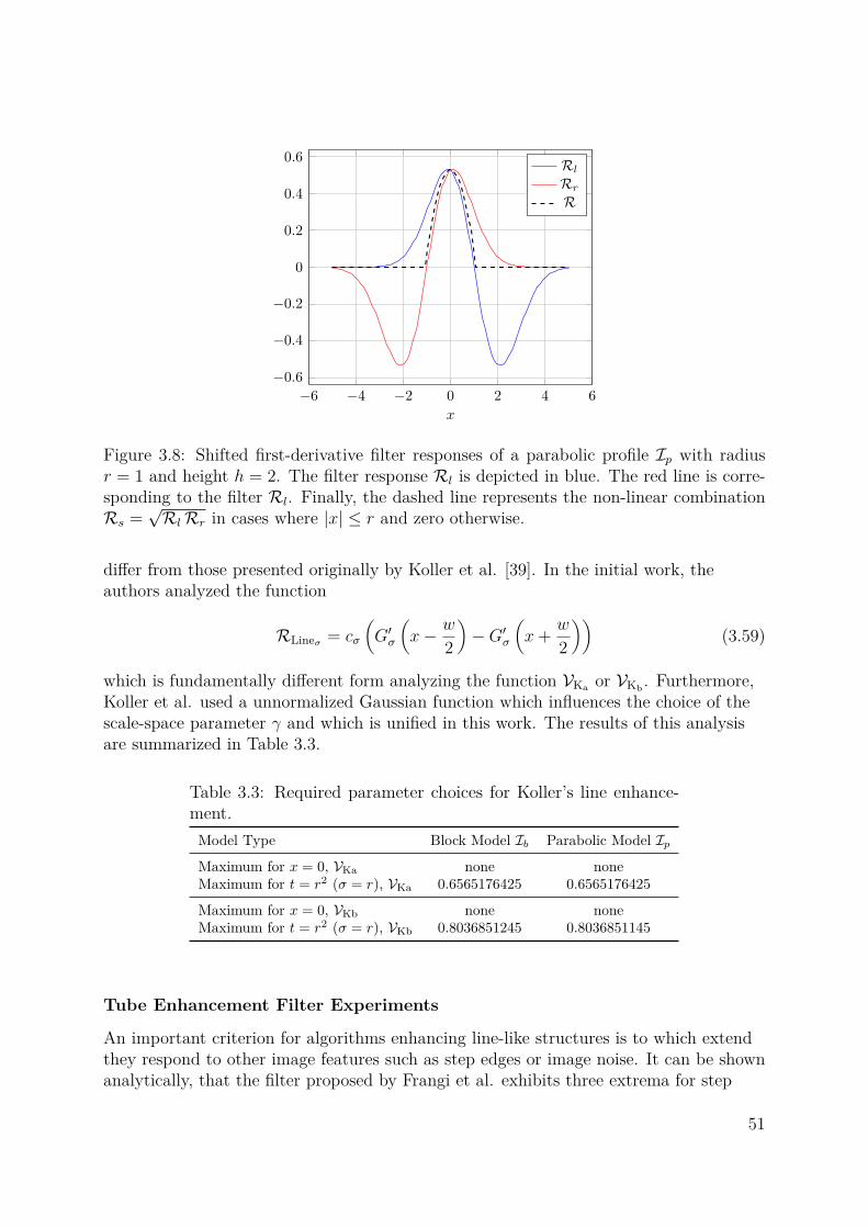
−6 −4 −2 0 2 4 6−0.6

−0.4

−0.2

0

0.2

0.4

0.6

x

Rl

Rr

R

Figure 3.8: Shifted first-derivative filter responses of a parabolic profile Ip with radiusr = 1 and height h = 2. The filter response Rl is depicted in blue. The red line is corre-sponding to the filter Rl. Finally, the dashed line represents the non-linear combinationRs =

√RlRr in cases where |x| ≤ r and zero otherwise.

differ from those presented originally by Koller et al. [39]. In the initial work, theauthors analyzed the function

RLineσ = cσ

(G′σ

(x− w

2

)−G′σ

(x+ w

2

))(3.59)

which is fundamentally different form analyzing the function VKa or VKb . Furthermore,Koller et al. used a unnormalized Gaussian function which influences the choice of thescale-space parameter γ and which is unified in this work. The results of this analysisare summarized in Table 3.3.

Table 3.3: Required parameter choices for Koller’s line enhance-ment.Model Type Block Model Ib Parabolic Model Ip

Maximum for x = 0, VKa none noneMaximum for t = r2 (σ = r), VKa 0.6565176425 0.6565176425

Maximum for x = 0, VKb none noneMaximum for t = r2 (σ = r), VKb 0.8036851245 0.8036851145

Tube Enhancement Filter Experiments

An important criterion for algorithms enhancing line-like structures is to which extendthey respond to other image features such as step edges or image noise. It can be shownanalytically, that the filter proposed by Frangi et al. exhibits three extrema for step

51

(a) Toy Example (b) Frangi et al. (c) Koller et al.

Figure 3.9: Filter responses on a toy example. The scale-space responses are computedwith the optimal σ values for the parabolic model. Scale values are ranging from 1 to 4and an overall of 21 scales were probed, i.e. t ∈ 1, 1.15, 1.3, . . . , 4.0.

edges. For a step edge Is defined as

Is(x, h) =

0 x ≤ 0h otherwise

(3.60)

the filter response becomes

V(x, t, γ, c, h) = 1− exp−exp

(−x2

t

)h2x2t−3+2γ

4πc2

. (3.61)

Computing the extrema of V(x, t, γ, c, h) depending on the variable x leads to threesolutions. These are

x ∈

0,+√t,−√t

. (3.62)

These additional responses on step edges can be observed as expected in the toyexample presented in Figure 3.9(b). The second filter discussed in this section does notexhibit such behavior on step edges. In fact, the nonlinear combination of the filter iseffectively suppressing these kind of edges. The toy example of Figure 3.9(a) containsfour edges on the horizontal and vertical image centers and these are suppressed in theresponse Figure 3.9(c). The remaining noise responses in the Figure 3.9(c) are hardlypossible to remove. In the bottom right square of the toy example which show a whitecurve on black background, Koller et al.’s filter produces spurious responses. However,these responses are according to what is modeled by the filter. Close to the crossing ofthe white lines, two of the path are approaching each other in a steep angle and thusstart acting as the borders of a dark line structure which is correctly detected by thefilter. A real world example of different filter responses is provided in Figure 3.10.The above analysis provides a simple derivation for properly configuring and using twoof the most popular feature enhancement algorithms. In particular, it was derived how

52

(a) Contrasted Brain Image (b) Frangi et al. (c) Koller et al.

Figure 3.10: Filter responses of a medical example. The input image on the left shows ahead in which the vessels supporting the brain are enhanced by contrast agent.

to properly normalize filter responses within the scale-space when using normalizedGaussian derivative filters base on Euqations 3.30 to 3.32. Especially Sato’s and Frangi’svessel enhancement filters are commonly used in medical applications. Both algorithmsare integrated in the well known and widely used Insight Toolkit [34]. From amathematical point of view, Frangi’s filter is an extension to Sato’s filter because it doesnot only include the structuredness but it is also modeling the blobness as the ratiobetween the smallest and largest eigenvalue. This additional term acts as an additionaldiscrimination factor to separate line-like from blob-like structures.Koller’s line enhancement algorithm on the other hand side seems still being lessaccepted as other alternatives. Here, it has been shown that the filter has severaladvantageous properties. First, the filter does not require any constraints on theminimal scale selection in order to ensure a maximal response on ridge tops and thisindependently of the ridge models analyzed in this work. Second, Koller et al.’s filterdoes not create any spurious responses on step-edges which means the method is causingless spurious responses. A third advantage is the fact that the filter does not require thechoice of an additional parameter and thus no individual tuning. However, the methodis not without problems though they are primarily of practical nature. Because the filterrequires the gradient projection onto ridge normals, the method requires to calculate theHessian and its eigendecomposition as well as the image gradient which is not needed forFrangi et al.’s filter. The result is a slightly worse run-time behavior. Overall, it hasbeen decided for this work, that the advantageous outweigh the run-time impact and itis suggested to favor the filter proposed by Koller et al.

3.3 Semi-Automatic DetectionIn Section 1.4.1 two modules for motion compensation are introduced. The first modeldeals with the initial tool detection and is designed to create a set of pixelsP = p1, . . . ,pM from a given key- or reference frame acquired at time tkey. In theoptimal case, this detection process would be fully automatic. However, currently nomethod for the fully automatic detecting of guide-wires in fluoroscopy exists which

53

(a) Overview (b) Close-up

Figure 3.11: Closeup of minimal initialization-graph with branching points.

produces results of sufficient accuracy [54]. In this section we present an approach forthe semi-automatic detection of guide-wires. The method is based on the second-orderstructural information contained in the images which has already been used for theenhancement of ridges. It utilizes the directional information provided by the Hessiananalysis to establish neighborhood relationships within the image and form a graph withpixels being the nodes where the graph’s edges connect neighboring pixels. Guide-wiresare then detected by manual selection of start- and end-nodes within this graph and bycomputing a shortest path [20] between these terminal nodes. The approach is similar tothe work recently presented by [67]. Other algorithms which motivated the developmentthis method are e.g. Livewire (also known as Intelligent Scissors) by Mortensen et al.[56] or the point linking method Steger [71, 70] proposes.In contrast to Livewire, the proposed method creates only a sparse graph of the pixelneighborhoods which results in faster processing. However, the presented approach mayin some cases result in segmentation failures because it may happen that the generatedgraph contains disconnected components. A prerequisite of Steger’s method is theexistence of multiple pre-detected sets of pixels, where it is assumed that all pixelsrepresent objects of interest. This is not the case for the method at hand. Here, it isrequired that two pixels on the curve are manually selected and the algorithm tries toestablish a connection between the selected points while being guided by image features.

Graph Creation

Here, an initialization procedure is proposed that requires the user to select two pointsclose to the extremities or end-points of a single medical tool. The basic idea is that thealgorithm tries to connect these two points by traversing pixels supposedly belonging tothe medical tool. In fact, the algorithm traverses a graph G = (V,E) with nodes Vcorresponding to individual pixels. The edges E of the graph are connecting neighboringpixels and to each edge ei ∈ E is a weight wi associated which is small for those edgesbelonging most likely to the medical tool.

54

Given two user-selected seed points s1 and s2, the system initializes a graphG1 = (V1, E1) with the seed point s1 as its first node, i.e. V1 = s1. Additionally to thegraph initialization, the node initializes a stack U = s1 of unprocessed nodes. Fromhere, the algorithm proceeds as follows. As long as the list of unprocessed nodes is notempty, i.e. U 6= , a node vc is popped from the stack U . For this node, up-to threeneighbors n1,n2 and n3 are selectively added to the graph G1. In case a node ni is notyet part of the graph, i.e. ni /∈ V1, it is added to the stack of unprocessed nodes and thestack becomes U = U ∪ ni. The weighted graph itself is extended by each neighbor nias

V1 = V1 ∪ ni (3.63)E1 = E1 ∪ (vc,ni, wi) . (3.64)

This growing process is continued until the stack U is empty and results in a first graphG1. In case the second seed point is already a part of the graph G1, one sets G = G1and continues with a single pair shortest-path computation. If s1 /∈ V1, the process isrepeated in the same way with the second, yet unprocessed seed point s2 which willresult in a graph G2 and the final graph G becomes G = G1 ∪G2. The final set of pixelsP = p1, . . . ,pM representing the medical tool is now computed as the solution of theshortest path problem on G for the node pair s1 and s2.Several question are now remaining. First, it needs to be defined how the neighborselection is working. Next, it needs to be discussed what happens in the aforementionedcase, when G1 ∩G2 = . This means, G consists of two disconnected components and inthis case a special fallback routine is required. Finally, computing shortest pathsrequires edge weights wi and it needs to be defined how to compute these weights.

Neighborhood Selection

During the graph creation process, a neighbor selection is required. It is claimed in theintroduction, that the method is utilizing directional information contained in the imagedata. As described in Section 3.2.1, the Hessian H of image intensities is providing therequired directional information. For any point vc being currently processed by thegrowing routine, the local Hessian matrix is analyzed. Its eigenvector tc correspondingto the smallest absolute eigenvalue is equivalent to the tangential direction of the curvein the point vc. Examples of such eigenvectors are represented by the green arrows inFigure 3.11(b).The directional information of the eigenvector or tangent is then used for the neighborselection in the following way. Assuming the tangent tc in the current point vc is definedas

tc =(txctyc

), (3.65)

where ‖tc‖ = 1, the corresponding direction α can be computed as α = atan2(tyc , txc ).This angle will fall into one of eight quadrants each spanning 45 and each defining asingle triplet of neighbors. The quadrants and the selected neighbors n1,n2 and n3 foran exemplary tangent direction are sketched in Figure 3.12.

55

−π + π8

−π2 −

π8 −π

2 + π8

−π8

π8

π2 −

π8

π2 + π

8

π − π8

r(√

32 , 1

2

)

Figure 3.12: Neighbor selection based on tangent direction t (corresponding to the redvector). The green squares indicate the selected neighbors.

Neighbor Saliency

As mentioned before, not all three candidate neighbors n1,n2 and n3 are added to thegraph but only salient ones. In order to accept all of the three following conditions musthold:

1. ni ∈ ΩI

2. V(ni) 6= 0

3. γ = arccos(‖〈tc, ti〉‖

)≤ 1

4π

The first condition is trivial and simply preventing the selection of invalid points byensuring the no points outside the image domain are chosen. The second condition isbased on any vesselness measure V introduced in Section 3.2.3. In case of Frangi’svesselness measure, V(nxi , n

yi ) is non-zero if and only if the largest eigenvalue of the

Hessian at point ni is positive which ensures that we are only tracing dark and line-likestructures. This can be seen from Equation (3.45) though it is defined for bright lines asopposed to dark lines which explains the negation of the relation. For Koller’svesselness, the feature value is non-zero when both side responses Rl and Rr arepositive (see also Equations (3.52) and (3.53)). The last condition ensures that theeigenvectors located at vc and ni are pointing in similar directions and do not deviateby more than 45. This is motivated by the assumption that the object we want tosegment exhibits certain smoothness.

56

Graph Dilation

The graph dilation is the aforementioned fallback routine which is used to deal withcases in which the created graph G consists of two disjunct components. How can thishappen? During the selection of salient neighbors, some neighbors are rejected. Inparticular problematic is the second saliency criterion which requires that V(nxi , n

yi ) 6= 0

holds for a candidate neighbor ni. Due to the noisy nature of interventional images anddue to the small size of the desired structures and partial occlusion by backgroundobjects such as ribs or the spine, guide-wires and other medical tools sometimes appearas disconnected objects. In cases where the object appearance is corrupted by noise, thecorruption are is most often caused by single pixels. This means, that beyond this singlecorrupted pixel, the object is again visible and leads to the idea to dilate the pixelgraph. So far, the neighborhood selection considers only direct eight-neighborhood of apixel vc. The dilation process relaxes this neighborhood selection by extending theneighbor search range.The method is performed by reconfiguring the graph growing such that the eighteenneighbor pixels around vc are investigated. Each of the leafs of graph G is pushed intoan empty stack U and the graph growing is run a third time which results in a newgraph G which may contain edges (vc, ni) of length up to 2

√2. This method is primarily

a heuristic approach giving the system a second chance to recover from initial failures.This indicates, that even after the graph dilation it is possible to face the situationwhere either s1 /∈ V or s2 /∈ V which prevent the computation of a shortest pathbetween the nodes s1 and s2. In such cases, the algorithm failed and the user is requiredto choose a different set of seed points s1 and s2 or a different input image I.

Edge Weights

Assuming, everything went fine and the graph G allows the computation of a shortestpath between the nodes s1 and s2 it is required to provide edge weights wi for every edgeei = (nj,nk, wi). Given the tangents tj and tk of the nodes nj = (nxj , n

yj ) and

nk = (nxk, nyk) and the feature image V , the edge weights wi are computed as

wi =(

1−√V(nj)V(nk)

)arccos

(‖〈tj, tk〉‖

). (3.66)

This measure leads to small values when the geometric mean of the vesselness measuresat locations nj and nk is high, i.e. when both pixel locations are likely to belonging to aline-like structure. Furthermore, the measure gets the smaller the smoother the curve is,which is modeled by the angle between the tangents tj and tk.Using these edge weights wi as defined above, it is possible to Dijkstra’s [20] shortestpath algorithm and to compute an ordered set

P = p1, . . . ,pM (3.67)

resembling the discrete points belonging to the desired medical tool.An overview of the basic algorithm without the second chance or graph dilation,respectively is provided in the pseudo-code algorithm 22.

57

3.4 Fully Automatic DetectionIn this section, two methods for the fully automatic detection of ridge like structures arediscussed. The first method is the result of the work of Carsten Steger [71, 70] and it isnot only detecting and linking edge points but also providing a classification of the pixeltype, i.e. whether the pixel is a center curve pixel, whether it is an end-point orbelonging to a junction. Furthermore, the method computes sub-pixel locations of ridgecenters and local tube widths. The second method that is presented in this section is amodification of Canny’s well known edge detection algorithm. The adaption replaces thegradient magnitude by a ridge indicator and adapts the non-maximum suppression in away that it is performed along ridge normals.

3.4.1 Canny Ridge DetectionThe well known edge detection method proposed by Canny [13] is originally based onthe computation of the image gradient ∇I. It uses the gradient magnitude ‖∇I‖ as an

Algorithm 1: Semi-Automatic Tool Detectioninput : Image I, Vesselness V , Tangents Toutput: Tool Pixels P

1 s1, s2 ← initializeSeedPoints();2 G← (V,E);3 for i← 1 to 2 do4 U ← si;5 while U 6= do6 vc ← pop(U);7 tc ← T (vc);8 N ← computeNeighbors();9 foreach ni ∈ N do

10 if ni ∈ V then continue;11 U ← push(ni, U);12 ti ← T (ni);13 γ ← arccos

(‖〈tc, ti〉‖

);

14 if ni ∈ ΩI ∧ V(ni) = 0 ∧ γ ≤ π/2 then15 wi ← computeEdgeWeight(V(nc),V(ni), γ);16 V ← V ∪ ni;17 E ← E ∪ (nc,ni, wi);18 end19 end20 end21 end22 P ← dijkstra(G, s1, s2);

58

(a) Canny Ridges (b) Steger Ridges

Figure 3.13: The figure shows two exemplary results of a fully automatic ridge detectionmethod. On the left-hand side, an approach derived from Canny’s edge detection algo-rithm has been used and on the right-hand side is the method of Carsten Steger. Bothmethods generate multiple responses and require additional post-processing to filter outspurious results.

indicator of edge strength. After the computation of the gradients and gradientmagnitude, the method starts by a non-maximum suppression in the direction of thegradient, i.e. orthogonal to edges. Gradients at a pixel location p are only then retainedwhen neighboring gradient magnitudes in the gradient direction ±∇I are both smallerthan the gradient magnitude located in the current pixel. This method is then followedby a hysteresis threshold based on two threshold values thigh and tlow, where the highthreshold value is used to select salient pixels and the low threshold is used to perform aregion growing starting from this pixel and including neighbors until their gradientmagnitude is greater or equal to the lower threshold. This method ensures, that theoutput of the detection algorithm are only a single pixel wide and in the originalmethod, these pixel sets are corresponding to edge locations.As opposed to Steger’s method (see below), Canny’s edge detection does not provideany ordering on the pixels nor any additional geometric information besides the factthat pixels are located on edges. Additional methods for linking pixels to line segmentsare required to generate this additional kind of information.The adaption to the detection of ridges is straight forward and requires only twomodifications of the original algorithm. First, the gradient magnitude needs to bereplaced with a measure which indicates high likelihood for pixels belonging to ridges asopposed to edges. Here, again any vesselness measure V of the previously mentioned(see Section 3.2.3) tube or ridge enhancement methods suffices. After the adaption ofthe salience measure, the gradient direction need to be adapted. Non-maxima need tobe suppressed orthogonal to the object of interest. For edges, this direction is

59

corresponding to the gradient

∇I =[Gx ∗ IGy ∗ I

], (3.68)

though for ridges this choice is not correct. Following the findings of Section 2.2, it isclear that again the directional information provided by the Hessian H of imageintensities can be used to determine the normal of the ridges – it is equal to theeigenvector p corresponding to the largest absolute eigenvalue. From a practical,run-time point of view it is no problem that now second-order derivatives of the imageare required since the data is already computed for during the generation of thevesselness V .Exemplary results of this detection algorithm are shown in Figure 3.13(a). The resultsindicate that additional post-processing methods are required to filter out spuriousresponses. But not only does this method create false positives but it is also notproviding a segmentation of the whole guide-wire but only parts of it. Even though itmay theoretically be possible to improve the results by careful tuning of the choice ofthe hysteresis parameters as well as the parameters which are required for thegeneration of the feature image V the results will most likely not be generally applicable.Consequently, so far the method requires additional user interaction in order to selectthe correct line-segments or at least for the verification of the segmentation results.

3.4.2 Steger Ridge DetectionIn his work on “An Unbiased Detector of Curvilinear Structures” [70], Carten Stegerproposes a method which is based on the saliency or vesselness measure introduced bySato et al. The algorithms consists of two phases, a first one which selects pointsforming ridges and a second phase in which these points are linked to lines.As in the “Canny Ridge Detection”, points are detected by combining a saliencymeasure in combination with a hysteresis thresholding. The saliency measure Stegerproposes is identical to the measure proposed by Sato et al. presented inEquation (3.39). Therefore, the algorithm is also bound to the same constraints asSato’s method and requires the same scale-space normalization and constraints on t.Table 3.1 summarizes these results and they are corresponding in general to the findingsof C. Steger. A minor difference is that the choice of σ (see Equation (10) in [70]) whichcorresponds to

√t should be tightened to2

σ >r√3. (3.69)

The basic idea of the saliency measure is derived from the commonly known secondderivative test. Given a stationary point, here the ridge top, the ridge profile I∗(x, r, h)is a local maximum (belongs to a bright line) when

∂I∗(x, r, h)∂2x

< 0 . (3.70)

2In the work of Carsten Steger, the tube radius is defined by w as opposed to r which is used in thiswork.

60

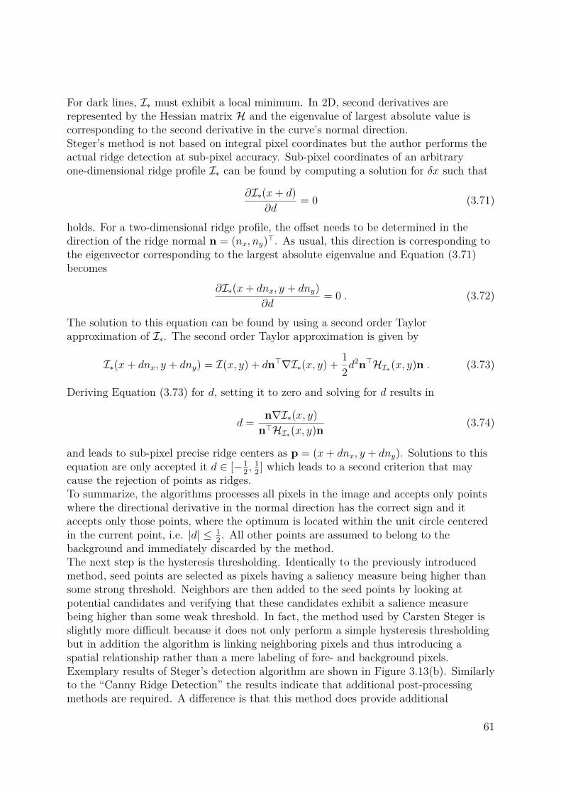
For dark lines, I∗ must exhibit a local minimum. In 2D, second derivatives arerepresented by the Hessian matrix H and the eigenvalue of largest absolute value iscorresponding to the second derivative in the curve’s normal direction.Steger’s method is not based on integral pixel coordinates but the author performs theactual ridge detection at sub-pixel accuracy. Sub-pixel coordinates of an arbitraryone-dimensional ridge profile I∗ can be found by computing a solution for δx such that

∂I∗(x+ d)∂d

= 0 (3.71)

holds. For a two-dimensional ridge profile, the offset needs to be determined in thedirection of the ridge normal n = (nx, ny)>. As usual, this direction is corresponding tothe eigenvector corresponding to the largest absolute eigenvalue and Equation (3.71)becomes

∂I∗(x+ dnx, y + dny)∂d

= 0 . (3.72)

The solution to this equation can be found by using a second order Taylorapproximation of I∗. The second order Taylor approximation is given by

I∗(x+ dnx, y + dny) = I(x, y) + dn>∇I∗(x, y) + 12d

2n>HI∗(x, y)n . (3.73)

Deriving Equation (3.73) for d, setting it to zero and solving for d results in

d = n∇I∗(x, y)n>HI∗(x, y)n (3.74)

and leads to sub-pixel precise ridge centers as p = (x+ dnx, y + dny). Solutions to thisequation are only accepted it d ∈ [−1

2 ,12 ] which leads to a second criterion that may

cause the rejection of points as ridges.To summarize, the algorithms processes all pixels in the image and accepts only pointswhere the directional derivative in the normal direction has the correct sign and itaccepts only those points, where the optimum is located within the unit circle centeredin the current point, i.e. |d| ≤ 1

2 . All other points are assumed to belong to thebackground and immediately discarded by the method.The next step is the hysteresis thresholding. Identically to the previously introducedmethod, seed points are selected as pixels having a saliency measure being higher thansome strong threshold. Neighbors are then added to the seed points by looking atpotential candidates and verifying that these candidates exhibit a salience measurebeing higher than some weak threshold. In fact, the method used by Carsten Steger isslightly more difficult because it does not only perform a simple hysteresis thresholdingbut in addition the algorithm is linking neighboring pixels and thus introducing aspatial relationship rather than a mere labeling of fore- and background pixels.Exemplary results of Steger’s detection algorithm are shown in Figure 3.13(b). Similarlyto the “Canny Ridge Detection” the results indicate that additional post-processingmethods are required. A difference is that this method does provide additional

61

information as geometric properties like the ridge width and ridge orientation as well assemantic properties where ridge pixels are classified as center pixels, end pixels or pixelsbelonging to junctions. It is not really an advantage because when looking at thealgorithm from a modular point of view, the same information can be added to the“Canny Ridge Detection”. This is not only true for the geometric and semanticproperties but also for the sub-pixel positioning of individual pixels. For future researchit might be beneficial to replace the salience measure used by Carsten Steger by thevesselness measure of Koller et al. because of its advantageous properties discussed atthe end of Section 3.2.3.

3.5 DiscussionIn this chapter, different methods for the enhancement and the semi-automatic as wellas fully automatic detection of medical tools were discussed. It turns out, that thesedays no method for the fully automatic detection of medical tools exists which performsat a level of reliability being required in clinical practice. Actually, it is most likely avalid assumption that simplified methods which operate only on single frames withoutthe consideration of temporal changes will not even in the future be capable ofperforming a segmentation at the desired level of reliability. From a practical point ofview this statement is strongly supported by the fact that even human observers havesometimes difficulties in detecting small structures in fluoroscopic image sequences whenthese do not exhibit any motion.Two ideas to tackle the problem in the future are presented in this section. In somesense both potential approaches considered here solve a classification problem. Recently,some authors [54, 33] proposed learning based algorithms for guide-wire detection and infact, these methods are already solving a fuzzy classification problem but one couldclaim that even hysteresis thresholding is a crude classification method. Moreinterestingly, both methods mentioned before do not yet utilize the time domain whichis in this work considered crucial for the development of fully automatic methods.Similarly to the image based methods presented in this chapter, the aforementionedlearning based methods mainly focus on appearance and intensity models.The incorporation of the time domain is considered important for future work and whatmost obviously changes in time is the spatial location of medical tools. For these objectstheir location is determined by the patient motion, dynamic changes of the projectiongeometry and tool interactions performed by the physician. One can observe thatbackground objects typically follow a different motion pattern than medical tools.Responses caused by image noise are unlikely to exhibit regular motion but can beassumed to follow random motion patterns. Other responses as e.g. the spinal discs as itis observed in abdominal interventions are hardly moving at all but remaining stationary.One possibility for the detection of medical tools within noisy background is spectralclustering [16, 83]. The method is based on the design of an affinity function which gluestogether objects belonging most likely to the same cluster. Given curvesCti (i = 1, . . . , n) and a method for tracking curves over time, it is possible to collect

spatial information for each curve Cti resulting in a set of curves

62

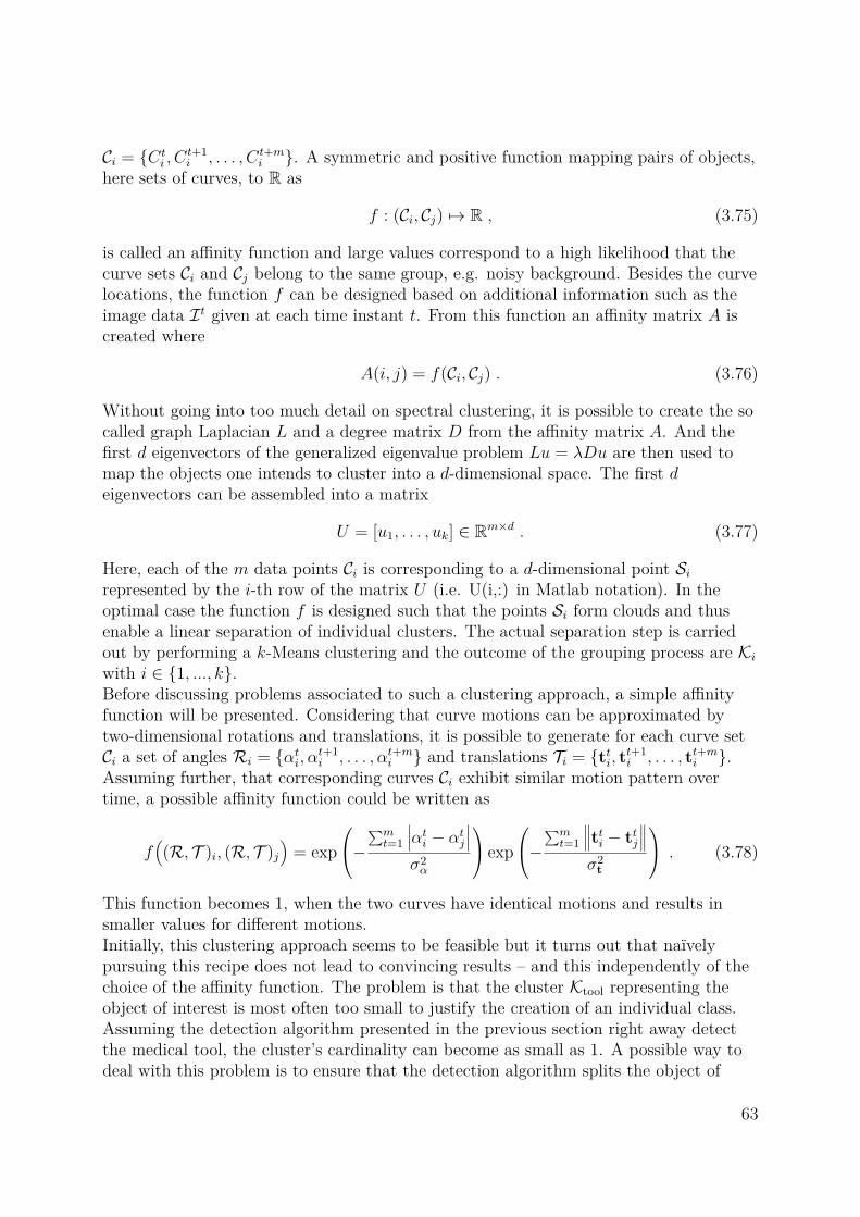
Ci = Cti , C

t+1i , . . . , Ct+m

i . A symmetric and positive function mapping pairs of objects,here sets of curves, to R as

f : (Ci, Cj) 7→ R , (3.75)

is called an affinity function and large values correspond to a high likelihood that thecurve sets Ci and Cj belong to the same group, e.g. noisy background. Besides the curvelocations, the function f can be designed based on additional information such as theimage data It given at each time instant t. From this function an affinity matrix A iscreated where

A(i, j) = f(Ci, Cj) . (3.76)

Without going into too much detail on spectral clustering, it is possible to create the socalled graph Laplacian L and a degree matrix D from the affinity matrix A. And thefirst d eigenvectors of the generalized eigenvalue problem Lu = λDu are then used tomap the objects one intends to cluster into a d-dimensional space. The first deigenvectors can be assembled into a matrix

U = [u1, . . . , uk] ∈ Rm×d . (3.77)

Here, each of the m data points Ci is corresponding to a d-dimensional point Sirepresented by the i-th row of the matrix U (i.e. U(i,:) in Matlab notation). In theoptimal case the function f is designed such that the points Si form clouds and thusenable a linear separation of individual clusters. The actual separation step is carriedout by performing a k-Means clustering and the outcome of the grouping process are Kiwith i ∈ 1, ..., k.Before discussing problems associated to such a clustering approach, a simple affinityfunction will be presented. Considering that curve motions can be approximated bytwo-dimensional rotations and translations, it is possible to generate for each curve setCi a set of angles Ri = αti, αt+1

i , . . . , αt+mi and translations Ti = tti, tt+1i , . . . , tt+mi .

Assuming further, that corresponding curves Ci exhibit similar motion pattern overtime, a possible affinity function could be written as

f((R, T )i, (R, T )j

)= exp

−∑mt=1

∣∣∣αti − αtj∣∣∣σ2α

exp−∑m

t=1

∥∥∥tti − ttj∥∥∥

σ2t

. (3.78)

This function becomes 1, when the two curves have identical motions and results insmaller values for different motions.Initially, this clustering approach seems to be feasible but it turns out that naïvelypursuing this recipe does not lead to convincing results – and this independently of thechoice of the affinity function. The problem is that the cluster Ktool representing theobject of interest is most often too small to justify the creation of an individual class.Assuming the detection algorithm presented in the previous section right away detectthe medical tool, the cluster’s cardinality can become as small as 1. A possible way todeal with this problem is to ensure that the detection algorithm splits the object of

63

interest into a reasonable amount of sub-segments. This can be achieved by separatingthe image I in the initial detection step into small sub-patches and by applying thedetection method on each of these sub-patches separately.Since the method proposed here is just a suggestion in which direction future researchmight continue, no evaluation has been performed. The recipe presented above is asimple way to incorporate information provided by the time domain. State of the artmethods aiming at the fully automatic detection of medical tools do not yet perform atan acceptable precision and stability suitable for clinical practice which leads to theconclusion that additional information is essential.

64

CHAPTER

FOUR

TOOL TRACKING

This chapter presents a novel method for the tracking of curves modeled by B-splines.In principle the tracking can be applied to open as well as closed curves thus enablingthe application of the method to segmentation problems where the B-spline is describinga contour as opposed to an open line-like structure. However, in this work the focus lieson medical tools and thus open curves.The tracking algorithm is based on discrete optimization methods and does not rely ongradient based formulations. This approach enables the utilization of complex modelsfor which derivatives can most often only be approximated by numerical methods. Suchnumerical differentiation methods are sometimes difficult to handle because they aresensitive to the discretization schemes, e.g. the step size at which derivatives areapproximated. This problem gets even more difficult for functions having a highdimensional parameter space and parameters which live in different sub-spaces as e.g.angles and translations which require different step sizes for a proper differentiation.One example where discrete optimization is beneficial and where derivatives can hardlybe estimated are energy terms of cost functions which are learned with offline data.Local minima, oftentimes caused by noise represent another problem which can bepotentially overcome by discrete optimization strategies. Because discrete optimizationmethods do not rely on gradient information, they lack strong forces keeping them fromleaving local minima and have the potential to discard such configurations and convergetowards a global optimum. Global optima in discrete optimization are slightly differentfrom those in continuous optimization because global refers to global within the discreteset of solutions. Especially for open curves, there exist discrete optimization strategiesthat are guaranteed to find the global optimum within the discrete set of solutions, i.e.that do not rely on any approximations.Nonetheless, also discrete optimization techniques are not without disadvantages.Gradient-based method intrinsically model interactions of different parameters. Fordiscrete optimization techniques which are based on graphs in which nodes representrandom variables and edges dependencies of these variables (or parameters) this wouldbe only guaranteed in cases where a node were connected to all nodes on which it isdepending. Such a procedure is in practical applications not feasible because it results in

65

an explosion of the computational complexity and therefore these interactions requireapproximative solutions. The efficient design of approximation schemes is an importanttopic in this work and will be discussed in this chapter.The first section of this chapter focuses on the modeling of curves and the modeling oftool motions. Afterwards, several possibilities for the modeling of objective functions arediscussed and defined as continuous functions which could potentially be used in anyoptimization framework. It is common that such cost function consist of at least twocomponents. A first component which drives the optimization and which is usuallyreferred to as data term or internal energy. These terms are usually based on somesaliency measures sometimes also called feature images or vesselness images in case ofline-like structures. The second term, the regularization is required to deal with theill-posedness of the optimization problem. Regularization terms are used to convexifyobjective functions and are often based on geometric observations. Several methods forthe regularization are reviewed in this chapter and a group of regularization schemes ispresented.After the introduction of the energy terms, MRFs are introduced and it is described howto use these optimization techniques for tracking. Section 4.3 goes into detail on how todiscretize the continuous functions presented in Section 4.2. Additionally, the section willprovide details on approximation errors related to an incomplete modeling of parameterinterdependency. Various approximation schemes are introduced and evaluated.The last part, Section 4.4 presents a variety of synthetic experiments which are inparticular used to support the validity of the approximation schemes. In addition, theexperimental section contains results on hand-labeled clinical data. The results show theapplicability of the method and its potential to correctly estimate the apparent toolmotion. Besides synthetic experiments and those on clinical data, the last sectioncontains a quantitative comparison of the proposed tracking algorithm with a recentlyintroduced learning based method.

4.1 Modeling of Guide-Wires and Needles

In this work, curves are modeled by non-uniform B-splines. The general form of a p-thdegree B-spline is

C(u) =m−1∑i=0

Ni,p(u)Pi , (4.1)

where u is a parameter defining the location on the curve. The curves which are used inthis work are not arc-length parameterized. In Equation (4.1), u = 0 and u = 1 arecorresponding to the curve’s end-points. The functions Ni(u) are different B-spline basisfunctions, each associated to a control point Pi. In this work, the objects of interest areobserved in two-dimensional images and thus the B-spline’s control points aretwo-dimensional as well, i.e. Pi ∈ R2. The i-th B-spline basis function of degree Ni,p(u)

66

is defined by

Ni,0(u) =

1 if ui ≤ u < ui+1

0 otherwise(4.2)

Ni,p(u) = u− uiui+p − ui

Ni,p−1(u) + ui+p+1 − uui+p+1 − ui+1

Ni+1,p−1(u) , (4.3)

which is usually referred to as the Cox-de Boor recursion formula [19]. This function isdefined by so called knots ui ∈ R and the augmented knot-vector

U = u0, u1, . . . , um+p . (4.4)

Augmented is here used because the first and last p+ 1 knots are equal to 0 and 1,respectively. For an augmented knot vector with n = m+ p+ 1 knots, the knots ui withi = p+ 1, p+ 2, . . . , n− p− 1 are referred to as internal knots.The utilization of B-splines is most common for the tracking of medical tools. In fact, allother works presented in Section 2.3 are using B-splines too. In general researchers tendto use uniform B-splines because they can be efficiently implemented since in thisspecial case, the basis functions are just shifted copies of each other. The uniformity of aB-spline curve is reflected in the distribution of the knots on the interval [0; 1] since inthe uniform case, the knots are uniformly distributed on that interval. From a practicalpoint of view, non-uniform distributions enable better approximation of curves whichexhibit strong local variations of curvature.

Fitting of Smoothing Splines: For the task of tracking, one is initially given a listof points

P = p1,p2, . . . ,pM (4.5)

by the detection module for which a spline function C(u) with a maximum of m controlpoints is sought after which obeys certain optimality criteria. The spline C(u) shouldapproximate the data by finding a compromise between a close fit and a smooth solutionin the sense that discontinuities in the curve’s p-th derivative should be as small aspossible. Dierckx [17, 19] proposes to formulate this problem in terms of the followingminimization:

Minimize η :=n−p−1∑i=p+1

(C(p)(u)(ui+)− C(u)(p)(ui−)

)2(4.6)

s.t. δ :=M∑j=1

wj(pj − C(uj)

)2≤ S (4.7)

In this equation C(p) is the p-th derivative with respect to u. An implementation of thismethod called parcur is publicly available in the library FITPACK [18]. It does notonly compute the optimal control points Pi but also allows for the computation of anon-uniformly distributed knot vector U . In this work, the weights for individual datapoints are set to wj = 1.

67

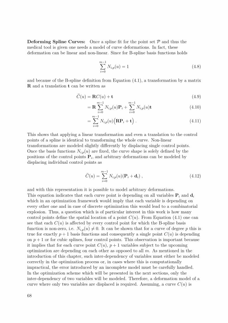
Deforming Spline Curves: Once a spline fit for the point set P and thus themedical tool is given one needs a model of curve deformations. In fact, thesedeformation can be linear and non-linear. Since for B-spline basis functions holds

m−1∑i=0

Ni,p(u) = 1 (4.8)

and because of the B-spline definition from Equation (4.1), a transformation by a matrixR and a translation t can be written as

C(u) = RC(u) + t (4.9)

= Rm−1∑i=0

Ni,p(u)Pi +m−1∑i=0

Ni,p(u)t (4.10)

=m−1∑i=0

Ni,p(u)(RPi + t

). (4.11)

This shows that applying a linear transformation and even a translation to the controlpoints of a spline is identical to transforming the whole curve. Non-lineartransformations are modeled slightly differently by displacing single control points.Once the basis functions Ni,p(u) are fixed, the curve shape is solely defined by thepositions of the control points Pi, and arbitrary deformations can be modeled bydisplacing individual control points as

C(u) =m−1∑i=0

Ni,p(u)(Pi + di) , (4.12)

and with this representation it is possible to model arbitrary deformations.This equation indicates that each curve point is depending on all variables Pi and diwhich in an optimization framework would imply that each variable is depending onevery other one and in case of discrete optimization this would lead to a combinatorialexplosion. Thus, a question which is of particular interest in this work is how manycontrol points define the spatial location of a point C(u). From Equation (4.1) one cansee that each C(u) is affected by every control point for which the B-spline basisfunction is non-zero, i.e. Ni,p(u) 6= 0. It can be shown that for a curve of degree p this istrue for exactly p+ 1 basis functions and consequently a single point C(u) is dependingon p+ 1 or for cubic splines, four control points. This observation is important becauseit implies that for each curve point C(u), p+ 1 variables subject to the upcomingoptimization are depending on each other as opposed to all m. As mentioned in theintroduction of this chapter, such inter-dependency of variables must either be modeledcorrectly in the optimization process or, in cases where this is computationallyimpractical, the error introduced by an incomplete model must be carefully handled.In the optimization scheme which will be presented in the next sections, only theinter-dependency of two variables will be modeled. Therefore, a deformation model of acurve where only two variables are displaced is required. Assuming, a curve C(u) is

68

displaced in the j-th and k-th control points, the deformed curve can be written as

C(u,dj,dk) = Nj,p(u)(Pj + dj) +Nk,p(u)(Pk + dk) +m−1∑i=0

i 6=j,i6=k

Ni,p(u)Pi

= C(u) +Nj,p(u)dj +Nk,p(u)dk . (4.13)

In the same way, it is possible to derive the displacement in three control points i, j andk as

C(u,di,dj,dk) = C(u) +Ni,p(u)di +Nj,p(u)dj +Nk,p(u)dk . (4.14)

The deformation model which is used in this work is slightly different than the onepresented in Equation (4.13). A problem caused by Equation (4.13) is the assumptionthat only two control points are moving while no other control point is changing itsposition. This assumption leads to intermediate curves C(u,dj,dk) which are onlyroughly approximating the reality. The fact, that in reality neighboring curve pointsexhibit a similar motion lead to the development of a new deformation model. In thenew model, the smoothness of the motion is incorporated by applying the displacementsof the control points Pj and Pk also to their neighbors. The resulting curve beingdisplaced by dj and dk is represented by

C(u,dj,dk) =j∑i=0

Ni,p(u)(Pi + dj

)+

m−1∑i=k

Ni,p(u)(Pi + dk

)

= C(u) +j∑i=0

Ni,p(u)dj +m−1∑i=k

Ni,p(u)dk . (4.15)

To summarize, the most important point of this section is that medical tools aremodeled with non-uniform B-splines. The non-uniformity improves the curve evaluationbecause it allows a linear sampling of the domain [0; 1] while preventing linearly spacedpoints on the curve – i.e. even though the domain is linearly sampled, curve points maycluster in areas of high curvature. A second important result is the way in which toolsare deformed which is described by Equations (4.14) and in particular (4.15). Regardingthe remaining details as e.g. the efficient evaluation of B-splines the reader is kindlyasked to refer to secondary literature [61, 19].

4.2 Modeling of Objective FunctionsIn the following, the general continuous formulation of the curve tracking problem isreviewed. Given an initial curve C, one wants to estimate transformation parametersleading to a new curve C∗ which is conforming with observed image data I.Mathematically, this means one seeks to maximize the posterior probability

C∗ = arg maxC∈F

P (C | I) , (4.16)

69

and in this equation C∗ is referred to as the MAP estimate. Based on Bayes’ theorem,which states that

P (C | I) = P (I |C)P (C)P (I) , (4.17)

Equation (4.16) can be rewritten. Assuming a constant P (I) is generally considered safeand since a constant factor does not affect the result of the maximization, the problemcan be rewritten as

C∗ = arg maxC∈F

P (I |C)P (C) . (4.18)

In this equation the term P (I |C) is referred to as the likelihood distribution and itevaluates how well a given curve C fits the observed image I. The second term P (C) iscalled the prior distribution and models potentially available a priori knowledge. In thecase of curve tracking this term can for instance be used to encode constraints on thegeometric appearance of a curve or prior knowledge regarding the type oftransformation one expects the curve to undergo. If no a priori knowledge is available,P (C) is assumed to be a uniform distribution where each curve configuration has thesame prior probability.Assuming furthermore, the probability distributions of Equation (4.18) follow a Gibbsdistribution with underlying energy functions, one can rewrite the MAP estimation asan energy minimization of the form

C∗ = arg minC∈F

E(I |C) + E(C) . (4.19)

In this case, one can interpret the likelihood energy E(I |C), often referred to as costfunction or data term, as measuring the quality of a certain model configuration.Likewise the prior energy E(C) can be interpreted as a regularization (or smoothness)term on the parameter space which allows to impose constraints on the solution.

External Energy When formulating the tracking problem based on B-spline curveswhich are defined on the interval [0; 1], the likelihood term (4.20) or external energy,driving the curve to its actual position can be formulated as

Eext(I |C) =1∫

0

ψ(I (C(u))

)du . (4.20)

Given that the image I is equal to one of the feature images V presented in Section 3.2,i.e. I = V , the function ψ is used to make the feature image’s values suitable forminimization. For a feature image with intensity values normalized to the interval [0; 1],this function can be defined as

ψ(I) = 1− I . (4.21)

When using such a function definition, the tracking problem is said to be modeled as animage based problem as compared to alternative, e.g. learning based models. In general,

70

image based methods differ only in the type of image I being used in Equation (4.20).To be more precise, the methods differ in the sort of pre-processing applied to the rawimage data. For the tracking of curvilinear objects, the most important image featuresare typically chosen as one of the earlier introduced ridgeness or vesselness measures[66, 22, 39].Several alternatives are possible too. In addition to Frangi’s vesselness filter [22], Baertet al. evaluated vesselness images on preprocessed input images in [3, 4]. Two types ofimages were evaluated. One with input images being pre-processed by some sort ofbackground removal and a second method where the input image was preprocessed withcoherence enhancing diffusion (CED) as proposed by Weickert [80]. According to theexperimental results of Baert et al. [3], Heassian feature images computed onunprocessed and pre-processed images lead both to a spline localization being similar tothe inter-observer variability. These results lead to the decision to ignore minimalpotential gains of these methods while preventing their inherent run-time penalties. Forthe same reason, other diffusion based filters such as the works of Canero et al. [12] andManniesing et al. [51] have not been adopted in this work.

Internal Energy The prior, which is also referred to as internal energy, constrainsthe motion of the curve. Regularization is well known and many regularization functionsare universally applicable for a multitude of problems. Constraints on B-splines whichpenalize geometric properties such as the curvature, length, or relative changes of thesevalues, are generically applicable to curve evolution algorithms.Another option for regularization is regarding the curve motions. In Equation (4.12),the curve motion is parameterized by displacements di for each control point. Similarlyto Equations (4.14) and (4.15), the deformation can be decomposed into the originalcurve C plus some deformation field D as

C(u) = C(u) +D(u) (4.22)

=m−1∑i=0

Ni,p(u)Pi +m−1∑i=0

Ni,p(u)di . (4.23)

These two curves have identical knots and differ only in their control points. A commonapproach is to ensure smoothness of the displacement field or to penalize deviations ofneighboring displacements. In fact, it is a common assumption that both approacheslead to the same results though this is not generally true. First, the displacement fieldone observes in this application is intrinsically smooth because it is a spline of degree pand thus Cp−1 continuous. Minimizing the distances of neighboring displacements leadsto a different effect causing the transformation to tend towards a pure translation. Inthe latter case, the spline D exhibits multiple identical control points di which leads to adegree reduction of the spline curve and thus to D being a straight line and finally aninfinitesimal point which is the same effect one achieves by minimizing the length ofD(u).Because of the natural smoothness of the displacement field, regularization approachestrying to explicitly enforce such a smoothness are considered to be needless for the task

71

of tracking and the focus will be laid on constraints of the curve’s geometry and itschanges over time.In this work, relative changes to initially observed data are considered in order toformulate the regularization. This is advantageous because it does not rely on fixedvalues which may be subject to changes caused by a different acquisition protocol orbecause of varying patient anatomy.Investigating the curve properties being acquired during the semi-automatic detectionphase results in reference data vinit which can be used to realistically constrain curvedeformations. Deviations of observed data values v from these values can then bepenalized by the squared relative error

ρ(v, vinit) =(

1− v

vinit

)2. (4.24)

During the development of the tracking algorithm, two possible ways of regularizing thecurve geometry were investigated. The first measure is based on length changescompared to a reference curve Cinit observed during the detection phase and the secondmeasure is penalizing deviations of the curvature between the currently observed curveC and the reference curve.In order to evaluate length changes, a mathematical formulation of a curve’s length isrequired and from differential geometry of curves it is known that for any given curve C,its length can be computed as

l =1∫

0

‖C ′(u)‖ du , (4.25)

where C ′ is the first derivative of the curve with respect to u. This follows, that lengthchanges can be penalized by

Elengthint = ρ

1∫0

‖C ′init(u)‖ du,1∫

0

‖C ′(u)‖ du . (4.26)

For reasons that will be justified later, it is desired to formulate energies as integrals ofsome error function and not like in Equation (4.26) as error functions taking integrals astheir parameters. Therefore, Equation (4.26) is reformulated and leads to the modifiedpenalty term

Elengthint =

1∫0

ρ(‖C ′(u)‖ , ‖C ′init(u)‖

)du , (4.27)

with ρ being defined as in Equation (4.24). This modification does not lead to the exactsame results but it is an acceptable approximation. In fact, it is even beneficial for thetracking because it helps to prevent a drift of the tracked curve along the observed one.The drift is oftentimes prevented because the measure forces tangent norms to be locallyequal.

72

The second penalty term measures differences of the curvature between the initial curveCinit and the currently observed one C. For a single point on the curve, the curvature iscomputed as

κ(C, u) =

∣∣∣C ′x(u)C ′′y (u)− C ′y(u)C ′′x(u)∣∣∣

‖C ′(u)‖3 . (4.28)

Here, the indices indicate which parameter is used (x for coordinates of the x-axis andvice versa y) and the primes indicate first- and second-derivatives of the curve C withrespect to u. Based on this equation, the penalty term can be written as

Ecurvatureint =

1∫0

ρ(κ(C(u)), κ(Cinit(u))

)du , (4.29)

This approach is not following the common methodology of minimizing the curvature toenforce smoothness. In case of B-splines, the inherent smoothness is often sufficient andterms such as the absolute value of the curvature can be discarded [15]. We are moreinterested in modeling the fact that the curve as seen at time instant t is similar to thecurve observed at a later point in time t+ n which is based on the assumption that thevessel-anatomy is not changing too much during the intervention.Experimental validation has revealed that the most important regularization componentduring the tracking is the length preserving term from Equation (4.27). Using thecurvature preservation alone is not sufficient because the measure is not scale variantand allows the curve to shrink or grow. Consequently, the only alternative to usinglength preservation only, is to combine both measures. Such an approach would lead tothe following energy function

Etotal = (1− λ)Eext + λ((1− γ)Elength

int + γ Ecurvatureint

)(4.30)

where λ and γ act as weighting factors from [0; 1] controlling the influence of externalversus internal energy and length versus curvature regularization, respectively.Exhaustive experiments have shown that introducing the curvature preservation does notlead to greatly improved tracking results. The main problem which arises when usingEquation (4.30) is the proper choice of the regularization weights λ and γ. To be moreprecise, even though it is possible to find specific parameters which work on a singlesequence, it is not necessarily true that the same parameters could be applied to anothersequence. These experiences lead to the choice of the follwoing energy formulation

Etotal = (1− λ)Eext + λElengthint . (4.31)

In continuous optimization, minimizing the above energies is commonly done in agradient descent approach. The initial contour is updated iteratively by computing thederivative of the energy function with respect to the model parameters. The algorithmstops if no further improvement on the energy can be achieved, meaning the methodconverges to a local minimum. Even if sometimes convenient to use, such an approach

73

CP1

P2

P3

P4

Lsparse Ldense

Figure 4.1: MRFModel of an open cubic B-spline curve C with control points Pi. A sparseand a dense version of the discrete set of labels L capturing the deformation space areillustrated (each black square corresponds to a displacement plus the zero-displacementat the control point position).

has two major drawbacks. First of all, the algorithm requires the derivation of theenergy term, which is oftentimes complex to calculate analytically and has to be donespecifically for every function. Second, a convergence to a good solution relies on thefact that the initial contour is sufficiently close. If the gradient descent starts far awayfrom the structure to be tracked, chances are high for obtaining bad solutions. This mayeasily happen in sequences with larger motion. Multi-resolution approaches (e.g.Gaussian scale space) might help in certain scenarios but do not overcome this generallimitation. Discrete optimization improves these issues and a strong indication is that inthis work, as opposed to previous works, no stratified approach is used (see alsoTable 2.1).

4.3 Markov Random Fields for TrackingSo far, this chapter provides a formulation of continuous energies which couldpotentially be minimized by using gradient based optimization. As mentioned earlier,this approach is difficult and can lead to problems. In order to overcome the limitationsof continuous optimization or at least in order to be able to diminish their influence, it isproposed in this work to render the tracking problem in a discrete framework.Discrete problems can be represented by so called probabilistic graphical models(PGMs). The entities required to build a PGM similar to the one presented inFigure 4.1 are nodes v ∈ V and edges e ∈ E which define a graph G = (V , E). The nodesof a PGM represent random variables of the problem being modeled which are linked byedges representing the variable interdependency. To be more general, G can even be ahyper-graph and in that case the edges e ∈ E are referred to as hyper-edges and maycontain more than just two nodes.Markov random fields (MRFs) are a special form of a PGM and belong to the class of socalled undirected graphical models (UGMs). Over the last years, MRFs have becomeincreasingly popular and the reasons for this raising popularity are two fold. First,MRFs are well suited for typical vision problems because the MRF graph structure isdirectly corresponding to the image structure which makes the modeling process

74

intuitive. Second, new methods for the efficient handling and solution of MRFs emergedrecently which allow to utilize these methods in real-world applications with demandingrun-time requirements.Let us consider a graph G = (V , E) consisting of a set of discrete variables or nodes Vand a set of edges E connecting neighboring pairs of variables in order to represent theirdependencies. Additionally, we introduce a discrete set of labels L capturing the searchspace of the model parameters. Each label xi ∈ L is associated with a two-dimensionaldisplacement vector dxi from the deformation space D ⊂ R2. Two possibilities for thediscretization of the deformation space are illustrated in Figure 4.1. If we associate eachcontrol point Pi of our B-spline model with one node of our graph, the task is to assignan optimal label to each of the nodes or a displacement to each of the control points,respectively. A common approach for modeling the labeling task in terms of energyminimization is the usage of first-order MRFs [45]

Emrf =∑i∈V

θi(xi) +∑

(i,j)∈Eθij(xi, xj) (4.32)

where θi are the unary potentials and θij are the pairwise potentials.In most applications, the unary terms play the role of the likelihood energy.Independently from all other nodes, the cost for an assignment of a certain label xi isevaluated. Then, the pairwise interaction terms play the role of regularization betweenneighboring nodes. However, the assumption that the likelihood of a labeling can becomputed from a sum of independent unary terms is actually not valid in our scenario.Considering B-splines with higher-order basis functions, the effect of a single controlpoint onto the deformation of the curve cannot be modeled independently from itsneighbors because the basis functions overlap. Therefore, a novel MRF model isproposed for the case of curve tracking using B-splines. First, the basis functions will beused as weighting coefficients within the energy terms. This leads to a higher influenceon the energy for curve points close to a certain control point as compared to theinfluence of points being farther away. A similar approach is used by Glocker et al. in[24] where the authors are using MRFs for non-rigid image registration based on cubicB-splines. Such a weighting allows a suitable approximation of the energy terms withrespect to the control points.In conventional modeling, external energies are represented by the unary terms ofEquation (4.32). This procedure imposes difficulties because it is based on theassumption that the energy is locally affected by a single node or control point whichwere only true when also the curve location were affected by a single control point. Ithas already been explained in Section 4.1 that this is not true for B-splines of degree pwhich are depending on p+ 1 control points.In order to improve this approximation, it is proposed to reformulate the externalenergy from the continuous domain as pairwise interaction terms and not as it iscommonly done as unary terms. Modeling the external energy as pairwise terms has bigadvantages. The non-vanishing interval of basis functions along the curve domain forcontrol point tuples is bigger than the corresponding interval of a single control point.Compared to unary potentials, the energy computation for the simultaneous movement

75

0 0.5 10

0.5

1

Unary – Ni(u)

0 0.5 10

0.5

1

Pairwise Sum – N+i,j(u)

0 0.5 10

0.5

1

Pairwise Product – N∗i,j(u)

Figure 4.2: Influence functions originating from an open cubic B-spline with seven controlpoints.

of a pair of control points yields a more accurate approximation of the continuousenergy. In the proposed approach both energies, the external and internal are defined aspairwise interaction terms as

Emrf =∑

(i,j)∈E

((1− λ) θijext(xi, xj) + λ θijint(xi, xj)

)(4.33)

where the discrete version of Equation (4.20) is build up by the pairwise terms

θijext(xi, xj) =1∫

0

Nij(u)ψ(I (Cij(xi, xj, u))) du (4.34)

and the internal energy from Equation (4.27) by all pairwise terms

θijint(xi, xj) =1∫

0

Nij(u) ρ(∥∥∥C ′ij(xi, xj, u)

∥∥∥ , ‖C ′init(u)‖)

du . (4.35)

Here, the weighting coefficient Nij(u) evaluates the influence of a curve point of the siteu to the energy of a control point pair (i, j) and the curve function Cij(xi, xj, u)describes the potential deformation of a curve when two control points i and j aredisplaced simultaneously by dxi and dxj , respectively. The potential deformation can becomputed efficiently by evaluating

Cij(xi, xj, u) = C(u) +i∑

k=0Nk(u) dxi +

m−1∑k=j

Nk(u) dxj , (4.36)

according to Equation (4.15).Regarding the influence functions Nij, two different versions are considered in this work.Either through the addition of basis functions which is called the sum model

N+ij (u) = Ni(u) +Nj(u)∑k+p−1

l=k Nl(u) +Nl+1(u)(4.37)

76

or through multiplication which is referred to as the product model

N∗ij(u) = Ni(u)Nj(u)∑k+p−1l=k Nl(u)Nl+1(u)

. (4.38)

Here, k is the index of the first non-zero basis function of a point C(u) and p is thedegree of the curve. The number of elements in the normalization terms (denominator)is solely depending on the curve’s degree because every point C(u) on a curve of degreed is defined by exactly p+ 1 control points, i.e. for every point p+ 1 basis functionsNl(u) are non-zero. The normalization is required in order to ensure that the discretizedversion (4.33) of the energy term is correctly approximating the continuous version fromEquation (4.31).Exemplary plots of these functions can be found in Figure 4.2. The curves in the middleand right-hand side plot can be interpreted as weighting functions for points belongingto curve segments defined by two control points. As can be seen in the section onexperiments in Table 4.1, the product model performs best. The reason is that thefunctions are steeper than those of the sum model. In other words one can say that thelocality of the product model is better than the one of the sum model.The performance of the two weighting functions is evaluated in Section 4.4.2 and theresults which include a comparison to the naïve approach where external energies aremodeled by unary potentials, i.e.

θiext(xi) =1∫

0

Ni(u)ψ(I (Ci(xi, u))) du , (4.39)

are summarized in Table 4.1.It is shown that the presented modeling of the tracking represents a good compromisebetween model accuracy and complexity. One could claim that the approximation errorcould be reduced (or even completely removed) if more complex models were used.However, the consideration of higher-order cliques as proposed by Ramalingam et al.[64] is even despite recent developments of Ishikawa [35] computationally tootime-consuming in order to be applicable in real-time environments.

4.3.1 OptimizationOnce the problem is formulated in a discrete setting, one needs to choose an MRFoptimization strategy. Fortunately, recent advances in discrete optimization brought acouple of very powerful techniques, mainly based on iterative graph-cuts or efficientmessage passing. Regarding the proposed model, there are two properties which shouldbe considered when using one of the existing techniques. First, for the special case ofopen curves the MRF graph from Figure 4.1 is a tree which allows the exactcomputation of the global optimal labeling when using max-product algorithms [60, 81](e.g. Belief Propagation, TRW-S [40]). Second, the energy is nonsubmodular which is a(theoretical) problem for some methods using graph-cuts [42]. Using certain truncationtechniques [65] on the energy terms make it still possible to use graph-cut based

77

techniques (e.g. Expansion Move [10]). Another possibility for minimizingnonsubmodular functions is described in [41] but this technique might result inunlabeled nodes which is not appropriate in the given setting. There are also methodsbased on iterative graph-cuts which can handle a wider class of MRF energies (e.g.Swap Move [10], FastPD [43]). Especially the FastPD algorithm is interesting in thiscase since a good performance with strong optimality properties is reported. InSection 4.4 the performance of the TRW-S and the FastPD algorithms are compared asrepresentatives for the message-passing and graph-cut approaches. As it turns out, asusual there is a compromise between speed and accuracy.

4.4 Experiments and EvaluationIn this section the performance analysis of the proposed tracking approach is presented.The evaluation consists of three parts. First, it is shown based on synthetic tests thatthe optimal influence function is the product model from Equation (4.38). Next, theinfluence of sparse as well as dense label sets is evaluated. In parallel to the label setsthe performance of fast but approximative optimization strategies is compared to exactthough slower strategies. For this analysis, TRW-S (exact), FastPD (approximative) andQPBO (approximative) were chosen as representatives for the two possible optimizationstrategies. The last part presents evaluations of the tracking algorithm on hand-labeledclinical data and a comparisons to the guide-wire tracking approach presented recentlyby Wang et al. [79].

4.4.1 Error AssessmentBefore continuing with the experiments the assessed error measures needs to be defined.A typically used error term for measuring the similarity of curves is the Hausdorffdistance

dH(C,CG) = max(

maxs

mintd(C(s), CG(t)

),

maxs

mintd(CG(s), C(t)

)). (4.40)

It is defined between a tracked curve C and the expected ground truth curve CG andinformally computes the maximal shortest distance between the two curves. Oneproblem is that the whole curve C could be displaced orthogonal by some vector oflength l and the Hausdorff distance would report the same error as for the case in whichboth curves were perfectly aligned with only a single pixel being off by a distance of l.In other words the distance measure does not handle outliers.Another issue is that the proposed method tracks guide-wire segments over time whilethe guide-wire itself is usually advanced further through the vessel system duringinterventions. As a consequence such a system may be initialized with curves beingsubstantially shorter than the ones observed later in the sequences. Since they arenonetheless labeled by experts during the generation of the ground-truth data, the

78

Hausdorff distance would report the length difference of the curves – even when thetracking were perfectly working.These constraints lead to the choice of a simple discretized and asymmetric errormeasure

d(C,CG, s) = mint

( ∥∥∥C(s)− CG(t)∥∥∥

2

)(4.41)

where one computes the minimal distance between the tracked and annotated curve.Evaluating Equation (4.41) at different sites s allows to compute statistics such as themean tracking error, its standard deviation or the median error.Similarly to what has been done in the work of Wang et al. [79] additional statistics arecomputed. These are the percentage of missed annotated pixels and the percentage offalse tracked pixels. The missed pixels are pixels of the annotation having a distance tothe tracked curve being higher than a specific threshold. Similarly, the false pixels arethose on the tracked curve being further away from the annotation as defined by thesame threshold. Conforming with previous works, the threshold is chosen to be equal to3 pixels.In the first case, regarding the missed pixels, the tracking failed to annotateground-truth data. It basically missed to highlight given data. An example when thisoccurs is exactly the case described before where the initial curve or tracked curve isshorter than the corresponding annotated curve. The second case, the false pixels arethose where the tracking computes a curve in locations where it actually does notbelong to. The algorithms is literally creating false or wrong results.

4.4.2 Approximation ErrorThe first experiment is evaluating different ways of diminishing our model inherentapproximation errors. In order to measure the influence of the approximation errorseveral tests are performed on synthetic data. The data is generated by randomlydeforming an initial open B-spline curve Cinit consisting of six control points. After thedeformation, an image frame is generated by careful rasterization of the deformed curveCt. Different sequences with different amount of deformations are generated and eachframe in every sequence is generated from the same initial curve Cinit.In this experiment the TRW-S [40] is used as the optimization method since it canrecover the global optimal solution for tree-like MRF topologies as they occur in theproposed model. By knowing that the exact ground truth spline Cinit is within thediscrete label space, it is possible to estimate the error induced by the energyapproximation only. Since furthermore each frame from every sequence is generatedfrom the exact same initial curve Cinit and since in this experiment the system isreinitialized with that specific curve in every frame, it is possible to discard theregularization term (i.e. set λ = 0) and thus an additional source which could bias theresults because regularization is mainly of interest in longer sequences where trackingerrors can accumulate over time.As mentioned before, different amounts of maximum deformations are used in eachsequence, ranging from 6 to 20 pixels control point displacements. Both proposed

79

model

max. def. unary pairwise sum pairwise product

6 1.00(±0.43) 0.34(±0.19) 0.28(±0.17)8 1.15(±0.52) 0.36(±0.23) 0.30(±0.19)10 1.33(±0.60) 0.42(±0.25) 0.36(±0.22)12 1.41(±0.70) 0.43(±0.27) 0.36(±0.23)14 1.74(±0.82) 0.48(±0.30) 0.43(±0.28)16 1.79(±0.93) 0.49(±0.32) 0.43(±0.29)18 2.00(±1.04) 0.52(±0.34) 0.47(±0.32)20 2.19(±1.15) 0.57(±0.40) 0.52(±0.34)

Table 4.1: Synthetic experiment which assesses theenergy approximation error under different amountsof deformation and three different likelihood models.Reported are the average curve distances and stan-dard deviations in pixels over one hundred frames persequence.

pairwise weighting functions, the sum model and the product model, are evaluated as wellas the naïve approach with unary potentials for the external energy. For a quantitativeevaluation of the synthetic results, the mean of the distances (and their standarddeviations) from Equation (4.41) at different, uniformly sampled sites s are evaluated.The results are summarized in Table 4.1. The product model performs best on allsequences. Especially, when considering larger deformations the approximation error hasa strong influence in case of unary potentials while both pairwise models still yield goodresults of always less than one pixel.

4.4.3 Deformation Space DiscretizationThe second experiment is intended to evaluate different discretization strategies as wellas the effect of approximative optimizers like the FastPD or QPBO. Since the number oflabels is an important parameter for the runtime of MRF optimization techniques, it isdesired to determine a reasonable compromise between speed and tracking accuracy.Two different strategies for discretization, a sparse one and a dense one, are proposed.They are visualized in Figure 4.1. Both versions are parametrized by two values, thenumber of sampling steps along a certain displacement direction and the range whichdefines the allowed maximum displacement. In case of sparse discretization, thedeformation space is sampled along eight directions, namely horizontal, vertical anddiagonal each in positive and negative direction. In case of dense sets, the completesquare space at a control point is sampled. Given the number of sample steps S, onegets |Lsparse| = 8S + 1, i.e. eight directions with S steps and in addition thezero-displacement. For the dense version one gets |Ldense| = (S + 1)2. Similar to the firstexperiment, eight synthetic sequences are generated by assigning uniformly distributedrandom displacements on the six control points of a given initial curve Cinit. Thedifference is that this time the ground truth is not covered by the label space. The range

80

of the label space is set to the maximum random deformation and different values forthe number of sampling steps are tested, namely 5, 10, and 20.

sparse dense

max. def. steps TRW-S FastPD QPBO TRW-S FastPD QPBO

5 0.32(±0.11) 0.44(±0.14) 0.35(±0.11) 0.30(±0.10) 0.41(±0.14) 0.33(±0.12)6 10 0.32(±0.11) 0.43(±0.13) 0.33(±0.11) 0.29(±0.10) 0.40(±0.12) 0.33(±0.12)

20 0.31(±0.10) 0.43(±0.13) 0.33(±0.12) 0.29(±0.10) 0.39(±0.13) 0.32(±0.11)5 0.42(±0.13) 0.59(±0.28) 0.48(±0.20) 0.37(±0.12) 0.53(±0.18) 0.43(±0.16)

8 10 0.41(±0.14) 0.56(±0.22) 0.45(±0.18) 0.35(±0.12) 0.48(±0.18) 0.40(±0.15)20 0.40(±0.14) 0.55(±0.22) 0.44(±0.17) 0.35(±0.12) 0.48(±0.17) 0.40(±0.14)5 0.52(±0.16) 0.76(±0.29) 0.61(±0.23) 0.48(±0.12) 0.69(±0.25) 0.57(±0.24)

10 10 0.51(±0.15) 0.74(±0.28) 0.59(±0.23) 0.43(±0.12) 0.66(±0.25) 0.54(±0.20)20 0.50(±0.15) 0.73(±0.29) 0.57(±0.18) 0.44(±0.12) 0.64(±0.26) 0.54(±0.22)5 0.62(±0.24) 0.87(±0.39) 0.72(±0.34) 0.53(±0.20) 0.75(±0.33) 0.65(±0.31)

12 10 0.60(±0.23) 0.84(±0.33) 0.69(±0.29) 0.50(±0.17) 0.70(±0.26) 0.64(±0.38)20 0.59(±0.22) 0.82(±0.33) 0.70(±0.33) 0.48(±0.16) 0.73(±0.38) 0.61(±0.36)5 0.75(±0.27) 0.98(±0.39) 0.85(±0.34) 0.59(±0.22) 0.86(±0.39) 0.75(±0.36)

14 10 0.71(±0.29) 0.93(±0.42) 0.84(±0.39) 0.56(±0.20) 0.82(±0.42) 0.71(±0.41)20 0.71(±0.28) 0.93(±0.44) 0.82(±0.38) 0.56(±0.21) 0.79(±0.46) 0.71(±0.39)5 0.91(±0.49) 1.30(±0.75) 1.13(±0.75) 0.69(±0.33) 1.17(±0.89) 0.95(±0.70)

16 10 0.88(±0.47) 1.34(±0.96) 1.04(±0.65) 0.67(±0.28) 1.24(±0.97) 0.98(±0.79)20 0.87(±0.48) 1.33(±0.89) 1.09(±0.68) 0.66(±0.29) 1.14(±0.89) 0.94(±0.77)5 1.11(±0.56) 1.47(±0.90) 1.26(±0.76) 0.89(±0.54) 1.34(±0.96) 1.22(±0.87)

18 10 1.07(±0.56) 1.42(±0.84) 1.20(±0.70) 0.84(±0.49) 1.29(±0.95) 1.18(±0.94)20 1.07(±0.59) 1.48(±0.90) 1.25(±0.77) 0.84(±0.51) 1.28(±0.93) 1.13(±0.84)5 1.16(±0.64) 1.54(±0.81) 1.38(±0.76) 0.96(±0.46) 1.37(±0.86) 1.20(±0.74)

20 10 1.09(±0.68) 1.52(±0.87) 1.27(±0.70) 0.85(±0.45) 1.40(±0.98) 1.16(±0.78)20 1.08(±0.63) 1.51(±0.84) 1.31(±0.69) 0.83(±0.38) 1.33(±0.95) 1.14(±0.69)

5 119.49 25.80 38.15 356.00 30.55 33.61run-time 10 493.13 39.53 51.42 > 4.5 · 104 71.22 70.07

20 1573.80 68.36 81.49 > 1.1 · 105 303.56 284.03

Table 4.2: Synthetic experiment for comparing the sparse and dense deformation spacediscretization. Run-times are reported in milliseconds and assessed on a 1.6 GHz IntelCore i7. All errors are reported in pixels. Throughout the experiment the FastPD wasconfigured with a maximum of 100 iterations and the QPBO with 2 outer sweeps.

Another difference is that the initial curve used during the tracking is not parameterizedin the same way as the curve used to generate the synthetic data. Therefore, theexperiment does not only reflect errors resulting from deformations which are notcovered by the label space but also those errors resulting from a sub-optimal curveparameterization.Again, we use the mean distance (and its standard deviation) as a measure of trackingquality. The TRW-S optimizer is chosen since it represents a state-of-the-art algorithmcomputing the optimal labeling for our energy term (recall that our MRF is a chain).On the approximative side, we chose the FastPD and QPBO because of their speed andgood optimality properties.

81

sequence name frames spacing deformation curve length

mean max mean max

cardiac 01 55 0.184 17 28 413 438cardiac 02 72 0.184 13 25 440 457cardiac 03 30 0.184 16 43 505 543cardiac 04 10 0.278 20 51 432 437cardiac 05 11 0.278 13 49 645 665abdominal 01 143 0.432 8 20 170 175abdominal 02 228 0.308 8 19 78 83

Table 4.3: Sequence Properties. The pixel spacing is given inmm and the deformation and length parameters are denotedin pixels.

category parameter

name value

spline modeling degree 3control points 12

discretization search steps 40 (321 labels)search range 15 (mm)

regularization λ 0.7

Table 4.4: Tracking Parameters.

Table 4.2 shows that the use of FastPD combined with sparse label sets is extremelyefficient and reasonable tracking accuracy can be achieved. Furthermore, it shows thatthe QPBO achieves tracking results which are even closer to the optimal ones whileintroducing a minor runtime penalty. The difference between sparse and dense label setsis quite small regarding the tracking error while in case of sparse sets we achieve nearreal-time performance in all experiments. Expectedly, the TRW-S gives the betterresults in terms of accuracy but it is not suitable for real-time applications. In the initialwork [31] these experiments lead to choosing the FastPD as the underlying optimizerwhich is now changed in favor of the QPBO.

4.4.4 Experiments on clinical dataIn the final experiment, the tracking is evaluated on 7 clinical sequences out of which 5are acquired during cardiac (diagnostic catheterizations) and 2 during abdominal(transarterial chemoembolization; TACE) interventions with an AXIOM-Artis 1 systemat a cine rate of 15 frames per second. The sequences contain an overall of more than500 frames and deformations of up to 50 pixels. More detailed properties of theindividual sequences can be found in Table 4.3.The cardiac data sets were made available to us by Wang et al. [79] and each of the

1Siemens Healthcare, Forchheim, Germany

82

sequence name mean standard deviation median

MRF-T RGWT MRF-T RGWT MRF-T RGWT

cardiac 01 (55 frames) 1.50812 1.66698 1.87401 1.63623 0.97893 1.17436cardiac 02 (72 frames) 1.52339 1.57126 2.71825 1.80749 0.70623 0.89453cardiac 03 (30 frames) 1.49126 1.29458 2.40836 1.50879 0.69463 0.730933cardiac 04 (10 frames) 0.84560 0.82023 0.92164 0.732867 0.61347 0.686065cardiac 05 (11 frames) 1.13857 1.33017 1.31548 1.4922 0.68615 0.817549

abdominal 01 (143 frames) 0.80728 n/a 0.63047 n/a 0.68212 n/aabdominal 02 (228 frames) 1.18741 n/a 1.37192 n/a 0.78049 n/a

Table 4.5: Experimental validation between the robust guide-wire tracking (RGWT)method of [79] and the proposed MRF based tracking (MRF-T). The last two rowsof the table show our method applied to two additional abdominal sequences whereno comparison with the robust guide-wire tracking was possible.

data sets did not only contain image data but also ground-truth annotations as well asthe tracking results of the author’s algorithm. The abdominal sequences were providedby our clinical partners; they were acquired during TACE interventions and as thecardiac sequences, hand-labeled by an expert.We use a single set of parameters (see Table 4.4) throughout all experiments. Theregularization weight is set to λ = 0.7 though Figure 4.3 indicates that other choices arepossible without severely decreasing the algorithm’s performance. The figure shows theresults of an experiment in which we evaluated the tracking error (the mean of false andmissed rates) for 100 different parameters λ and for each medical sequence.The labeling is configured with a search range of 15 mm and 40 search steps in eachdirection resulting in an overall of 321 labels per node. The sparse labeling is chosenaccordingly to Section 4.4.3 and following the results of Section 4.4.2 the product modelis used as our influence function.Regarding the algorithm run-time, it is useful to split the overall processing into twosteps. The first step, before the optimization is carried out, is the computation of thefeature image I and the second step is the actual optimization process. We havemeasured a mean processing time of about 33.52 ms (σ = 13.06 ms) for the computationof the feature image I and a mean optimization time of 26.22 ms (σ = 9.60 ms). Thisresults in an overall of about 60 ms processing time. With these processing rates this isto the best of our knowledge the first algorithm which is capable of processingfluoroscopic images at the same rate as they are acquired by the imaging system.A summary of the comparison between the two methods can be found in Tables 4.5 and4.6. The experiments show that our method is performing on average equally well ascompared to the robust guide-wire tracking (RGWT) by Wang et al. [79] while it is notrelying on any learning. Visual results of the tracking performance are depicted inFigure 4.4. The results show that the tracking may suffer from the introduction of localloops and foldings in areas of high curvature but it also shows corresponding imagesfrom the same sequences in which the algorithm recovered from such intermediateerrors. The first row of Figure 4.4 shows in particular the robustness to poor features

83

sequence name missed false

MRF-T RGWT MRF-T RGWT

cardiac 01 (55 frames) 10.7778 12.213 15.6204 13.5093cardiac 02 (72 frames) 7.14789 11.3662 7.65493 9.94366cardiac 03 (30 frames) 8.86207 9.18966 9.87931 11.1552cardiac 04 (10 frames) 3.11111 1.44444 2 0.61111cardiac 05 (11 frames) 9.1 10.3 8.8 11.85

abdominal 01 (143 frames) 1.86972 n/a 4.1338 n/aabdominal 02 (228 frames) 6.14537 n/a 18.7489 n/a

Table 4.6: Experimental validation between the robust guide-wire tracking (RGWT) method of [79] and the proposed MRFbased tracking (MRF-T). The last two rows of the table showour method applied to two additional abdominal sequenceswhere no comparison with the robust guide-wire tracking waspossible.

0 0.1 0.2 0.3 0.4 0.5 0.6 0.7 0.8 0.9 10

10

20

30

40

50

60

70

80

90

100

λ

erro

r

cardiac 01cardiac 02

cardiac 03

cardiac 04

cardiac 05

abdominal 01abdominal 02

Figure 4.3: The plot shows the evaluation of the regularization parameter λ and itsdependency on the mean of false and missed tracking rates. The plot indicates that awide variety of parameter choices is possible without dramatically hampering the trackingquality.

where the algorithm is capable of maintaining correct curve shapes despite the lack ofimage information.

84

(a) fluoro - cardiac 01 (b) noisy feature image I (c) guide-wire annotation

(d) fluoro - cardiac 04 (e) too sparse label set (f) tracking recovered

(g) fluoro - abdominal 01 (h) folded curve) (i) tracking recovered

(j) fluoro - abdominal 02 (k) looped curve (l) tracking recovered

Figure 4.4: Tracking results from selected clinical sequences. The first row shows thatthe algorithm is able to deal with noisy feature images and the remaining rows depictthe sources of intermediate tracking errors – a too sparse label set, foldings and theintroduction of loops. In all three cases, the algorithm was capable of recovering fromthese errors.

85

CHAPTER

FIVE

A SIMPLIFIED MOTION COMPENSATION SYSTEM

In this chapter, the current status of an integrated motion compensation system ispresented. The work which is described in this chapter has been carried out in closecollaboration with the Siemens Healthcare Angiography/X-Ray division (AX) located inForchheim, Germany and Siemens Corporate Research (SCR) in Princeton, New Jersey.The presented motion compensation system has been integrated into InSpace, a volumeimaging application shipped with many radiologic hardware products of Siemens. Theapplication allows the addition of new software modules in form of plug-ins which canbe developed in C++ and added to any existing system.The motion compensation module’s structure can be described at best with three layers.A first layer is the actual core application hosting the plug-in, i.e. InSpace itself.InSpace provides the infrastructure for loading different plug-ins, for generating userinterfaces and most importantly for accessing medical image and meta data. The secondlayer is the actual plug-in. It is used to leverage the infrastructure provided by InSpacein order to allow user interactions and for the generation of a user interface. Besides theuser interface and interaction, the plug-in implements a control loop in which the dataflow between InSpace and the underlying algorithmic component is handled. The thirdlayer is build by the actual algorithms for guide-wire, catheter and needle detection aswell as the tracking and motion estimation.

5.1 Plugin DesignSince the plug-in was designed as a research tool and not a clinical product it does notonly contain dialogs which would be required in clinical routine. The additionalinterfaces allow to modify the visualization, e.g. the blending between thetwo-dimensional fluoroscopic image sequence and three-dimensional image data. It alsoallows the specification of offline data instead of being bound to online data which isimportant to be able to evaluate different methods on identical data sets. Regarding theonline processing of data in principle only a single user input is required which allowsthe user to manually enter the detection phase where user interactions are requiredwhich are in general not available.

87

Another requirement during the design of the plug-in was the ability to interchangedifferent tracking algorithms. To achieve this a generic programming interface wasdesigned which allows different researchers to implement individual approaches to solvethe detection, tracking and motion estimation. The implementation is provided in formof a so called dynamic library which is loaded during the run-time by the plug-in, i.e.from within the second layer. This approach allows a seamless exchange of theunderlying library and thus the used algorithms and improves future maintainabilitybecause it separates the application interface from the underlying algorithmiccomponents. The developed interface is provided in Listing C.1.The interface has been designed based on the subsequent reasons. Starting with therequirements, it can be assumed that a motion compensation system needs to providethe following functionality

1. algorithm configuration

2. initialization

3. tracking

4. data exchangeand these items have been directly translated into the design of the interface. Anotherimportant factor is a strong decoupling of the second layer, i.e. the plug-in and thealgorithmic component. Its definition must not impose dependencies on user specificdata types but should be solely build upon fundamental data types or aggregates ofthese. This constrained is fulfilled on the one-hand side by creating an interface which isbased on simple and well defined objects. On the other-hand side, a specialimplementation method, the Pimpl idiom [72] has been used. It allows to move allimplementation details into a separate object which does not require to be exposed tothe end-user. This procedure allows to provide an implementation of the abovefunctionality without introducing additional dependencies. It reduces the interface to anabsolute minimum of pre-defined objects.The interface which is provided for the first point, the algorithm configuration assumesthat all kinds of algorithms can be setup through a single configuration file. This shouldeven be true for learning based algorithms which do not only need to provide generalalgorithmic parameters but also offline learned data and other prior information.So far, the second point, the initialization is a semi-automatic method. Thus it requiresnot only images and the associated meta data but also the data generated by the userinteraction. Currently, this data is simply a set of two user selected points but in orderto be flexible in regard to potential extensions, the data is encapsulated in a separateclass.For the actual tracking a slightly different approach has been chosen in the sense thatthe interface does not allow to provide additional information besides the evidentlyrequired image data. The reasoning here is that even for complex algorithms,customizations are performed either internally or the required data is provided duringthe configuration phase. It is assume unlikely that a use case exists which explicitlyrequires the plug-in layer to provide dynamic information during the course of tracking.

88

The last point is regarding the data exchange. So far, only two use-cases are considered.First, it is of interest to visualize the tracking results and thus the interface providesfunctionality to retrieve the locations of tracked curves. Second, the plug-in layerrequires information regarding the actual motion the curves performed. Thisinformation is provided in form of a two-dimensional transformation even though thepresented algorithms actually compute dense deformation fields. The reason is that atthe moment not all components of the system envisioned in Section 1.4 are availablewhich lead to the development of an intermediate and simplified visualization system.

5.2 Visualization ComponentBecause the current work is only dealing with the third component presented inSection 1.4, which is the motion compensation within a fluoroscopic image sequence, afully featured navigation system cannot yet be provided. Instead a simpler approach foraiding physicians during their navigation task is chosen. The approach chosen in thiswork is based on the rigid alignment of a roadmap image Imap and the currentlyobserved fluoroscopic image It. This is either possible by applying a rigidtransformation Tt provided by the motion estimation to the roadmap image Imap, or

Figure 5.1: The image shows a screenshot of InSpace. The top-left view is used to displaythe actual fluoroscopic image stream including a DSA as its roadmap overlay.

89

alternatively the inverse transformation to the fluoroscopic image It.All choices presented here assume that the alignment between the roadmap image Imapand a key-frame Itkey is known and without loss of generality this transformation isassumes to be the identity transformation. The required roadmap image can be createdin one of the following ways:

1. Based on a 3DRA: Given a pre-interventionally acquired 3D-RA, it is possibleto create a projection image Imap with the same projection geometry as the one ofa fluoroscopic image sequence. 3D-RAs are reconstructed from native X-rayimages generated by a calibrated C-arm system. The projection is possiblebecause the 3D image as well as the 2D image sequences are generated by thesame system in which all projections are performed relative to a commoncoordinate frame. Modern robot controlled system do not only allow highprecision positioning of the X-ray source and the digital detector but also enableto read out the required pose information.

2. Based on a DSA: Alternatively to 3D-RAs, the generally acquired DSA can beused as a roadmap image. As opposed to the usage of a 3D-RA, the DSA must begenerated with the same projection configuration as the fluoroscopic sequence inorder to be able to overlay the images. Potential zooming which is oftentimes usedduring fluoroscopic runs can be compensated by an additional scaling andtranslation of the two-dimensional image data and the required transformationinformation is provided by the C-arm systems.

Both approaches suffer from the same problem – once the two-dimensional roadmapimage is generated Imap the question remains how to choose the correct key-frame Itkeyfrom the fluoroscopic image sequence. The issue is that the choice is not arbitrary sinceone needs to find a reference image which is optimally corresponding to the roadmap,i.e. with an underlying physical patient geometry being as close as possible to the onefrom which the roadmap was generated. A first step towards a similar patient geometryis to find a fluoroscopic image which is acquired in the same phase of the breathing cycleas the roadmap image Imap. In Section 1.4, this task is meant to be solved within theDeformable 2D-2D Registration Module. For the task of finding a fluoroscopic imageItkey corresponding best to a given DSA a straight forward approach were to select theimage which correlates best to the native X-ray image based on which the DSA wasgenerated. The so chosen image Itkey is the best candidate one can find to pursue themissing 2D-2D registration in order to compensate additional deformations.The only component which is missing to finalize the plug-in visualization is the actualcomputation of the rigid transformation Tt which relates the guide-wire locations Ptkeyof the key-frame to the currently observed image It. To this end, a method for theleast-squares estimation of transformation parameters between two points sets which isproposed by Umeyama [76] is used. In his work Umeyama shows that for two points setsX = x1,x2, . . . ,xn and Y = y1,y2, . . . ,yn, the transformation that minimizes

ε2(R, t) = 1n

n∑i=1‖yi − (Rxi + t)‖2 (5.1)

90

can be computed from the covariance matrix of the demeaned point sets

Σxy = 1n

n∑i=1

(yi − µy)(xi − µx)> . (5.2)

and the corresponding mean values µx and µy. Having computed the solution to thisproblem, for points sets Ptkey and Pt, one gets

Tt =[Rt tt0 1

]. (5.3)

Based on the above description a motion compensation system has been built andintegrated into InSpace. Figure 5.1 shows a screenshot of the system including atransformed image It such that it optimally fits a DSA roadmap.

91

CHAPTER

SIX

CONCLUSION

This thesis introduces novel methods for the semi-automatic detection of medical toolssuch as guide-wires, catheters or biopsy needles. Furthermore, the work presents for thefirst time an approach which solves the tracking problem for B-spline curves based ondiscrete optimization. The focus of this work lies on clinical applications being guidedby fluoroscopic imaging. In particular the method has been evaluated on abdominaldata sets acquired during transarterial chemoembolization (TACE) and five clinicalcardiac sequences.The development of the semi-automatic detection method which is based on sparsegraphs induced by the second-order structure of image intensities does not only allow arobust but also a fast segmentation of curvilinear structures. Since full featuredapplications usually consist of processing pipelines containing several algorithms at once,run-time reduction while retaining stable algorithms is an important topic.A new tracking approach which is based on a MRF formulation represents the maincontribution of this work. The problem is formulated as finding a solution to a discretelabeling problem which has recently received increasing attention in many early visionproblems. In contrast to the common approach applied in vision problems, in whichMRF nodes correspond to the image lattice this work proposes to model MRF nodes ascontrol points of a B-spline curve. Such curves can be either open curves representingcurvilinear structures such as e.g. medical tools or they can be close curves asparameterizations of object contours. This implies that the approach is not limited totracking but maybe as well applied to segmentation problems.One of the main advantages of discrete optimization is that it is currently considered asone of the most-powerful techniques to minimize non-convex functions. Especially in thescenario of tracking curves in fluoroscopic image sequences non-convexity is a potentialproblem. All image based data terms rely on feature images highlighting curvilinearstructures in one or the other way and these methods have no way of distinguishingbetween bone interfaces and thin medical tools. As it can be seen in the examples inFigure 3.13, the images contain many line-like structures which can potentially attractthe curves and cause local minima.Another advantageous property of MRF based methods is that they do not rely on

93

gradients. This property makes it possible to use a large variety cost functions withoutbeing able to provide analytical derivatives and without worrying about performance orstability degradations that might be caused by numerical differentiation. This allows forinstance to use learning based measures which offer the potential of further increasingtracking stability.Experiments have shown that the proposed method is performing at high-precision.This is true for multiple sequences which are even acquired during differentinterventional procedures (abdominal and cardiac). Furthermore, experiments analyzingthe behavior of the regularization revealed that the algorithm is relative stable within acertain parameter range. Last but not least, the procedure is running near real-timebeing faster than other tracking systems being presented so far without necessarilyrequiring a rigid pre-registration.

6.1 DiscussionBesides the just presented advantages the approach is not without difficulties. Oneproblem is the incomplete modeling of the inter-dependency of individual randomvariables. This problem leads to intermediate curves C(u,dj,dk) which onlyapproximate the expected curve as it is depicted in Figure 6.1. Careful handling of thisapproximation via weighting functions (Equations (4.37) and (4.38)) diminishes theissue but does not completely solve it.In the configuration depicted in Figure 6.1, a source curve consisting of control points Sibeing rotated by 15 to a target curve Ti is displaced in the control points S1 to S4 withthe expected displacements of S2 and S3 repectively. This results in and intermediatecurve where I1 = S1 + (T2 − S2), I2 = T2, I3 = T3, I4 = S4 + (T3 − S3) and I5 = S5. Sucha configuration is exactly what were evaluated by θ23

ext and θ23int from Equations (4.34)

and (4.35). The problem in this case is evident in Figure 6.1. Despite the correctdisplacements being applied the control points S2 and S3 of the source curve, theintermediate approximation does not overlap with the target.

S1 S2 S3 S4 S5T1

T2

T3

T4

T5

I1 I2

I3 I4

I5

Figure 6.1: Approximation Errors of Intermediate Curves.

Even though a perfect alignment is not necessary it can still lead to difficulties andhamper the convergence properties. There are two possible reasons, why the perfectintermediate alignment is not required. First, even though thin, medical tools have a

94

specific width, i.e. it exists a corridor around the target curve in which the externalenergy is non-zero and where the intermediate curve does result in an energy responsewhich drives the optimization towards the correct solution. The second potential reasonis that the optimization algorithm can solve the problem by initially assigning wrongintermediate results. In fact, such results will be tested and even assigned as long asthey result in a reduced energy. Since the optimization is an iterative process, upcomingiterations can fix the initially wrong result.Again, there may occur a potential problem with the latter solution of choosing actuallywrong intermediate results. It arises from certain regularization terms. In theory it mayhappen that wrong intermediate labels are the only way to reduce the external energybut on the other hand side such labelings may vastly increase the internal energy. Anexample is a regularization term penalizing transformations varying from rigidtransformations. In case such a cost function would be evaluated on the actual splinepoints the intermediate labeling would be penalized by the regularization.Unfortunately, the situation is rather difficult to evaluate because in this case the dataterm and regularization are acting against each other.The issues above were raised for the sake of clarity and to increase awareness. Theexperimental section has proven the effectiveness of the method and should encouragefuture researchers to utilize the possibilities offered by discrete optimization frameworks.

6.2 Future Work

In this section an alternative learning based tracking method is provided. The work hasbeen developed in collaboration with Olivier Pauly and Nassir Navab [59]. In principlethis work proposes to replace the external energy function defined in Equation (4.20) byanother function which is learned from hand-labeled offline data. The proposedmodification also leads to a slight modification of the original discretization (seeEquation (4.34)).The main idea of the approach is that instead on relying on feature image intensities Valong the curve profile C(u), a curve descriptor is extracted from the unprocessed imageI. To this end, so called mean orthogonal intensity profiles are used. They represent arelatively simple descriptor for curves and the external energy can be seen as measuringthe deviation from an observed descriptor to a learned and expected descriptor.Figure 6.2 shows a spline curve and the close-up of a ground-truth spline segment(dashed red curve) as well as a displaced spline segment (solid red curve). In theclose-up view, the top-right plot shows the mean orthogonal profile of the ground-truthcurve (green) and the mean orthogonal profile of the displaced curve (red).As it is expected from the derivation provided in Sections 3.1.2 and 3.1.3, theground-truth curve’s model is similar to a parabolic model. However, the model is notidentical since it is not symmetric in the sense that the intensities on both sides of themedical tool are varying. For such cases, learning based methods are advantageousbecause they make no prior assumptions on the actual model though they do rely on alearning database which provides the whole variety of possible curve appearances.

95

Figure 6.2: The left-hand side picture shows a guide-wire with a curve segment (dashedred line). The curve segment corresponds to the part of the guide-wire which is influencedby two neighboring control points. The right-hand side image shows a close-up with atransformed spline segment and equally sampled orthogonal profiles. The top left showsthe mean profiles of the ground truth as well as the displaced curve segment.

For a curve segment Cij(xi, xj, u) orthogonal line segments of length 2r are defined as

Nij(xi, xj, u, r) = Cij(xi, xj, u) + rn(u) (6.1)

where n(u) is corresponding to the normal of the curve segment Cij at the site u. Amean intensity profile can then be defined as

Mij(xi, xj, r) = 1|supp(Cij)|

∫supp(Cij)

r∫−r

I(Nij(xi, xj, u, r)) dr du . (6.2)

The mean profiles are only parameterized by the control points i and j as well as thenormal radius. Given a curve C(u) with m control points one can compute exactlym− 1 profiles with neighboring control points which build the input data set

M =Mi,i+1|i = 0, 1, . . . ,m− 2

(6.3)

whose elements are later evaluated by the learned cost function.The goal is now to learn a function ψ which maps local mean orthogonal profilesMij ∈M to a real values corresponding in some way to the expected tracking error, i.e.ψ is defined as

ψ : M 7→ R , (6.4)

where M is the set of mean orthogonal profiles. Since such a function should be convexand smooth, a thorough sampling of the space M is required. In [59] it is proposed tolearn a probability distribution corresponding to typical guide-wire motions from

96

hand-labeled sequences to ensure a proper sampling of M. Once the probabilitydistribution is available it is possible to create random curve displacements exhibitingtypical guide-wire motions. Such a sampling allows the generation of pairs of meanintensity profiles and the associated errors

(Mi,i+1, εi)k

(6.5)

on which a regression can be performed to learn the actual function ψ. Details on thelearning of typical guide-wire motions and the regression learning can be found in [59].The actual pairwise data term is then computed as

θij(xi, xj) = ψ (Mij(xi, xj, r)) . (6.6)

Preliminary results have shown that the method is feasible for the tracking ofguide-wires in fluoroscopic sequences. Sub-pixel precision was achieved in differentexperiments with different profile radii of r = 5mm and r = 10mm on two abdominaldata sets. The experiments were carried out by learning on one abdominal sequence andperforming the tracking on the other and vice versa. The advantage of the method isthat no pre-processing of the images is required and no prior assumptions on the modelare required since its appearance is learned.Despite the integration of a learning based cost function into a discrete framework, thework also proposes a second novel idea. Initially, the high-dimensionality of the featurespace M posed a problem since it severely complicates a meaningful sampling of thespace in order to generate data for the learning process. This problem has beenovercome by fitting a mixture of Gaussian model to hand-labeled deformations which inturn allows the random generation of deformations which are likely to occur in reality.Future improvements can be achieved by exploring the possibility of an adaptedregularization term which could be e.g. derived from the motion distribution model.Another improvement can probably be achieved by integrating the weighting functionsintroduced in Equation (4.38). So far these are ignored and as it has been shown in thisthesis, they may increase the performance of the algorithm even further.

97

APPENDIX

A

AUTHORED AND CO-AUTHORED PUBLICATIONS

1. Bender, F., Groher, M., Khamene, A., Wein, W., Heibel, T. H., andNavab, N. 3D dynamic roadmapping for abdominal catheterizations. InInternational Conference on Medical Image Computing and Computer AssistedIntervention (New York, USA, September 2008)

2. Groher, M., Bender, F., Khamene, A., Wein, W., Heibel, T. H., andNavab, N. 3D guide wire navigation from single plane fluoroscopic images inabdominal catheterizations. In Bildverarbeitung in der Medizin (2009)

3. Heibel, T. H., Glocker, B., Groher, M., Paragios, N., Komodakis, N.,and Navab, N. Discrete tracking of parametrized curves. In IEEE Conference onComputer Vision and Pattern Recognition (2009)

4. Heibel, T. H., Glocker, B., Paragios, N., and Navab, N. Needle trackingthrough higher-order MRF optimization. In IEEE International Symposium onBiomedical Imaging (2010)

5. Pauly, O., Heibel, T. H., and Navab, N. A machine learning approach fordeformable guide-wire tracking in fluoroscopic sequences. In InternationalConference on Medical Image Computing and Computer Assisted Intervention(2010)

6. Platonov, J., Heibel, T. H., Meier, P., and Grollmann, B. A mobilemarkerless AR system for maintenance and repair. In International Symposium onMixed and Augmented Reality (2006)

7. Traub, J., Heibel, T. H., Dressel, P., Heining, S., Graumann, R., andNavab, N. A multi-view opto-xray imaging system: Development and firstapplication in trauma surgery. In International Conference on Medical ImageComputing and Computer Assisted Intervention (2007)

8. Platonov, J., Heibel, T. H., and Meier, P. Camera position andorientation determining method for use in e.g. production area, involves projecting

99

data model of virtual information with preset camera parameters and findingcurrent parameters using external values of cost-function. Patent No.DE102005025470 (A1), 2006

9. Navab, N., Traub, J., and Heibel, T. H. Method for calibration of a cameraaugmented c-arm. Patent No. WO2009077480 (A1), 2009

10. Glocker, B., Heibel, T. H., Navab, N., Kohli, P., and Rother, C.Triangleflow: Optical flow with triangulation-based higher-order likelihoods. InEuropean Conference on Computer Vision (Crete, Greece, September 2010)

11. Wang, L., Springer, M., Heibel, T. H., and Navab, N. Floyd-WarshallAll-Pair Shortest Path for Accurate Multi-Marker Calibration. In InternationalSymposium on Mixed and Augmented Reality (October 2010)

100

APPENDIX

B

MATHEMATICAL EXTENSIONS

B.1 Enhancement of Tubular Structures

B.1.1 Sato’s and Frangi’s Feature Enhancement

The following equations represent the analytic expressions of Sato’s and Frangi’s featureenhancement in the pq-coordinate frame which are used in Equation (3.39) andEquation (3.46), respectively. Equation (B.1) is corresponding to the block model Ibwhich is defined in Equation (3.10) and Equation (B.2) corresponds to the parabolicmodel Ip defined by Equation (3.12).

Hpp(x,t, γ, r, h) = − 1√2√π

(

exp(−(r + x)2

2t

)tγ−

32h(

exp(2rx

t

)(r − x) + r + x

) )(B.1)

Hpp(x,t, γ, r, h) = −exp

(− rx

t

)tγ−1h

πr2√

2

(

πt√

2 exp(rx

t

)(erf

(r + x√

2√t

)+ erf

(r − x√

2√t

))−

2√t√πr

(exp

(−r

2 + x2

2t

)+ exp

(−r

2 − 4rx+ x2

2t

)) ). (B.2)

The γ value provided in Table 3.1 and Table 3.2 results form the following analyticalexpression

γ = 1√

2√

e√π erf

(12

√2)− 2

. (B.3)

101

B.1.2 Koller’s Feature EnhancementThe following equations represent the analytic expressions of Koller’s featureenhancement in the pq-coordinate frame which are used to compute Equations (3.50)and (3.51). The formulas are computed as Ix = Gx ∗ I∗.

Ix(x,t, γ, r, h) = − 1√2√π

(√

2 exp(−(r + x)2

2t

)tγ−

12h(

exp(2rx

t

)− 1

) )(B.4)

Ix(x,t, γ, r, h) =exp

(− rx

t

)tγh

πr2√

2

(√

2πx exp(rx

t

)(erf

(r + x√

2√t

)− erf

(r − x√

2√t

))+

2√t√π

(exp

(−r

2 − 4rx+ x2

2t

)− exp

(−r

2 + x2

2t

)) )(B.5)

The actual formulas Rl and Rr are computed as

Rl(x, t, γ, r, h) = Ix(x−√t, t, γ, r, h) (B.6)

Rr(x, t, γ, r, h) = −Ix(x+√t, t, γ, r, h) (B.7)

where Ix is chosen as Equation (B.4) for the block model Ib and as Equation (B.5) forthe parabolic model Ip.The analytic equations for the γ values presented in Table 3.3 are defined below.

γ = 12

e2 + 1e2 − 1 (B.8)

γ = −12

4√π +√

2 erf(√

2)πe2 − 4

√πe2

2√π +√

2 erf(√

2)πe2 − 2

√πe2

(B.9)

γ = −12

erf(√

2)2πe4 + 3

√2√π erf

(√2)

e2(1− e2)− 8e4 + 4e4 + 4

erf(√

2)2πe4 + 2

√2√π erf

(√2)

e2(1− e2)− 4e4 + 2e4 + 2(B.10)

Above, Equation (B.8) is the optimal γ for the block model Ib for both non-linearfunctions defined in Equations (3.52) and (3.53). The last two Equations are the γvalues of the parabolic model Ip belonging to Equations (3.52) and (3.53), respectively.

102

APPENDIX

C

CODE SAMPLES

Listing C.1: Minimalistic but generic interface for tracking which allows the implementa-tion and evaluation of various approaches.class MotionEstimationpublic:

/** Member variable initialization. */MotionEstimation();

/** Implements memory cleanup. */~MotionEstimation();

/** System configuration via configuration file. */void ConfigureSystem(const char *configuration_file);

/** Curve detection with an image and potential user interactions as its parameters. */void Detection(const ImageContainer& image, const DetectionParameter* detection_parameter = 0);

/** Tracking based on the current image and meta data. */void Tracking(const ImageContainer& image);

/** Retrieval of two-dimensional rigid motion data. */void GetMotionEstimate(float& x, float& y, float& angle) const;

/** Retrieval of detected curves. */void GetGWCurves(GWCurve const*& curves, int& no_curves) const;

/** Optional system reset to recover from errornous states. */void Reset();

private:/* Copying or cloning as well as assigning of the class are prohibited. */MotionEstimation(const MotionEstimation&) MotionEstimation& operator=(const MotionEstimation&) return *this;

int m_numberOfCurve; // Holds the number of tracked/detected curves.GWCurve* m_curves; // Holds tracked curves in form of point sets.

struct MotionEstimationImpl; // Forward declaration of the implementation.MotionEstimationImpl* m_pImpl; // A pointer to the implementation.

;

103

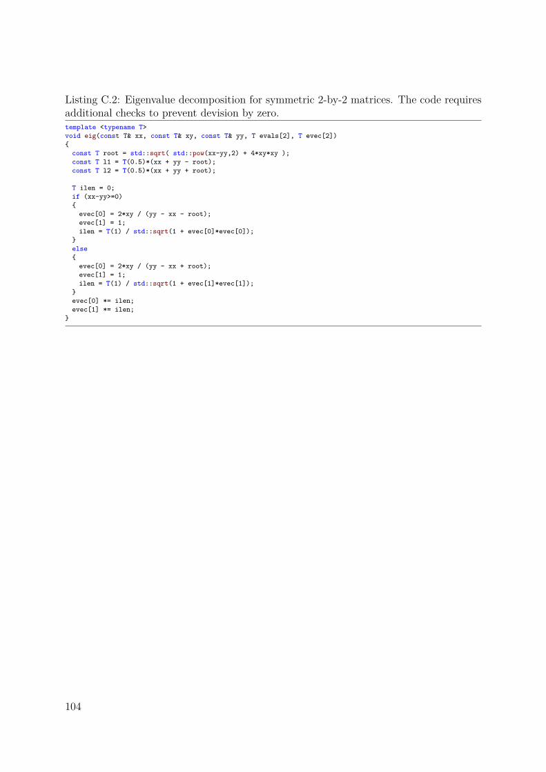
Listing C.2: Eigenvalue decomposition for symmetric 2-by-2 matrices. The code requiresadditional checks to prevent devision by zero.template <typename T>void eig(const T& xx, const T& xy, const T& yy, T evals[2], T evec[2])

const T root = std::sqrt( std::pow(xx-yy,2) + 4*xy*xy );const T l1 = T(0.5)*(xx + yy - root);const T l2 = T(0.5)*(xx + yy + root);

T ilen = 0;if (xx-yy>=0)

evec[0] = 2*xy / (yy - xx - root);evec[1] = 1;ilen = T(1) / std::sqrt(1 + evec[0]*evec[0]);

else

evec[0] = 2*xy / (yy - xx + root);evec[1] = 1;ilen = T(1) / std::sqrt(1 + evec[1]*evec[1]);

evec[0] *= ilen;evec[1] *= ilen;

104

LIST OF FIGURES

1.1 Most common 2D image modalities in interventional radiology. . . . . . . . 71.2 Computed Tomography Angiography (left) and Magnetic Resonance An-

giography (right). . . . . . . . . . . . . . . . . . . . . . . . . . . . . . . . . 91.3 Angiographic intervention setup. The monitor shows a live X-ray video

stream (left) next to a DSA (right) which serves as a roadmap during theintervention. The object on the left-hand side of the image is a flat-paneldetector from a modern C-arm system. . . . . . . . . . . . . . . . . . . . . 10

1.4 Components of interventional navigation. . . . . . . . . . . . . . . . . . . . 12

3.1 Idealized X-ray projection of a tubular object. The object is centered at C.The path lengths at which X-rays are attenuated in the tubular object varywith the projection direction α. The path length is denoted as l(cx, cy, r, α)and two examples for α = 0 and α = 8 are shown in red. . . . . . . . . . . 34

3.2 Idealized intensity responses of a tubular object with a radius r = 1 whichis located at a distance of 1 (i.e. c2

x + c2y = 1) to the X-ray source. The

plot shows the responses for a constant incident intensity of I0 = 1 forvarying attenuation coefficients µ. The functions correspond to the outputof Equation (3.9). . . . . . . . . . . . . . . . . . . . . . . . . . . . . . . . . 36

3.3 The figure shows optimal fits between three different ridge models and theidealized block model derived in Section 3.1.2. The models are (from left toright), a symmetric block model, an elliptical model and a Gaussian model.The red curves represent the optimal models after fixing the width to theexpected value while the green curves show the optimal models after fixingtheir height to the expected value. . . . . . . . . . . . . . . . . . . . . . . . 38

3.4 The two graphs in this figure depict a ridge model as it is generated byEquation (3.9). The left-hand side figure displays the model as a three-dimensional surface and the right-hand side figure show the correspondingtwo-dimensional gray-scale image. The red coordinate system with axes pand q represents the second-order gauge coordinates which are intrinsic tothe image surface. . . . . . . . . . . . . . . . . . . . . . . . . . . . . . . . . 40

105

3.5 The figure shows the vesselness response of the filter proposed by Sato etal. for a block model Ib(x, 2, 2) with width and height equal to 2. The ditchfor small scale-space values of t and x = 0 indicates, that the responses arenot meaningful for all scale-space parameters. . . . . . . . . . . . . . . . . 46

3.6 This plot shows the effect of the choice of the parameter c for Frangi’sstructuredness measure 1 − exp

(− S2

2c2

). When c is chosen too small, the

filter responses of neighboring but large values of S are hard to distinguish. 483.7 Comparison between Frangi’s vesselness enhancement with different scale-

space normalization constants. The images were created with scales σi ∈0.5, 1.5, 2.0 and 1.5σi. The scale-space normalization constants are com-puted according to Equation (3.49). . . . . . . . . . . . . . . . . . . . . . . 49

3.8 Shifted first-derivative filter responses of a parabolic profile Ip with radiusr = 1 and height h = 2. The filter response Rl is depicted in blue. The redline is corresponding to the filter Rl. Finally, the dashed line representsthe non-linear combination Rs =

√RlRr in cases where |x| ≤ r and zero

otherwise. . . . . . . . . . . . . . . . . . . . . . . . . . . . . . . . . . . . . 513.9 Filter responses on a toy example. The scale-space responses are com-

puted with the optimal σ values for the parabolic model. Scale valuesare ranging from 1 to 4 and an overall of 21 scales were probed, i.e.t ∈ 1, 1.15, 1.3, . . . , 4.0. . . . . . . . . . . . . . . . . . . . . . . . . . . . . 52

3.10 Filter responses of a medical example. The input image on the left showsa head in which the vessels supporting the brain are enhanced by contrastagent. . . . . . . . . . . . . . . . . . . . . . . . . . . . . . . . . . . . . . . 53

3.11 Closeup of minimal initialization-graph with branching points. . . . . . . . 543.12 Neighbor selection based on tangent direction t (corresponding to the red

vector). The green squares indicate the selected neighbors. . . . . . . . . . 563.13 The figure shows two exemplary results of a fully automatic ridge detection

method. On the left-hand side, an approach derived from Canny’s edgedetection algorithm has been used and on the right-hand side is the methodof Carsten Steger. Both methods generate multiple responses and requireadditional post-processing to filter out spurious results. . . . . . . . . . . . 59

4.1 MRF Model of an open cubic B-spline curve C with control points Pi.A sparse and a dense version of the discrete set of labels L capturingthe deformation space are illustrated (each black square corresponds to adisplacement plus the zero-displacement at the control point position). . . 74

4.2 Influence functions originating from an open cubic B-spline with sevencontrol points. . . . . . . . . . . . . . . . . . . . . . . . . . . . . . . . . . . 76

4.3 The plot shows the evaluation of the regularization parameter λ and its de-pendency on the mean of false and missed tracking rates. The plot indicatesthat a wide variety of parameter choices is possible without dramaticallyhampering the tracking quality. . . . . . . . . . . . . . . . . . . . . . . . . 84

106

4.4 Tracking results from selected clinical sequences. The first row shows thatthe algorithm is able to deal with noisy feature images and the remainingrows depict the sources of intermediate tracking errors – a too sparse labelset, foldings and the introduction of loops. In all three cases, the algorithmwas capable of recovering from these errors. . . . . . . . . . . . . . . . . . 85

5.1 The image shows a screenshot of InSpace. The top-left view is used to dis-play the actual fluoroscopic image stream including a DSA as its roadmapoverlay. . . . . . . . . . . . . . . . . . . . . . . . . . . . . . . . . . . . . . . 89

6.1 Approximation Errors of Intermediate Curves. . . . . . . . . . . . . . . . . 946.2 The left-hand side picture shows a guide-wire with a curve segment (dashed

red line). The curve segment corresponds to the part of the guide-wirewhich is influenced by two neighboring control points. The right-hand sideimage shows a close-up with a transformed spline segment and equallysampled orthogonal profiles. The top left shows the mean profiles of theground truth as well as the displaced curve segment. . . . . . . . . . . . . 96

107

108

REFERENCES

[1] Atasoy, S., Groher, M., Zikic, D., Waggershauser, T., Marcus, P., andNavab, N. Real-time respiratory motion tracking: Roadmap correction for hepaticartery catheterizations. In SPIE Medical Imaging (2008).

[2] Baert, S., van de Kraats, E. B., van Walsum, T., Viergever, M. A.,and Niessen, W. J. Three-dimensional guide-wire reconstruction from biplaneimage sequences for integrated display in 3-D vasculature. IEEE Transactions onMedical Imaging 22 (2003), 1252 – 1258.

[3] Baert, S., Viergever, M. A., and Niessen, W. J. Guide-wire trackingduring endovascular interventions. IEEE Transactions on Medical Imaging 22, 8(Aug. 2003), 965–972.

[4] Baert, S. A. M. Guide wire tracking and reconstruction in interventionalradiology. PhD thesis, University Medical Center Utrecht, 2003.

[5] Baert, S. A. M., Niessen, W. J., Meijering, E. H. W., Frangi, A. F.,and Viergever, M. A. Guide wire tracking in interventional radiology. InComputer Assisted Radiology and Surgery (2000).

[6] Baert, S. A. M., van Walsum, T., and Niessen, W. J. Endpoint localizationin guide wire tracking during endovascular interventions. Academic Radiology 10(2003), 1424–1432.

[7] Barbu, A., Athitsos, V., Georgescu, B., Böhm, S., Durlak, P., andComaniciu, D. Hierarchical learning of curves application to guidewirelocalization in fluoroscopy. In IEEE Conference on Computer Vision and PatternRecognition (2007), IEEE Computer Society.

[8] Bender, F., Groher, M., Khamene, A., Wein, W., Heibel, T. H., andNavab, N. 3D dynamic roadmapping for abdominal catheterizations. InInternational Conference on Medical Image Computing and Computer AssistedIntervention (New York, USA, September 2008).

109

[9] Bender, F. T. Segmentation, 2D-3D registration and uncertainty propagation fordynamic roadmapping in angiographic interventions. Master’s thesis, TechnischeUniversitüt München, 2007.

[10] Boykov, Y., Veksler, O., and Zabih, R. Fast approximate energyminimization via graph cuts. IEEE Transactions on Pattern Analysis and MachineIntelligence 23, 11 (2001), 1222–1239.

[11] Can, A., Shen, H., Turner, J. N., Tanenbaum, H. L., and Roysam, B.Rapid automated tracing and feature extraction from retinal fundus images usingdirect exploratory algorithms. IEEE Trans. Inf. Technol. Biomed. 3, 2 (1999),125–138.

[12] Canero, C., and Radeva, P. Vesselness enhancement diffusion. Pattern Recogn.Lett. 24, 16 (2003), 3141–3151.

[13] Canny, J. A computational approach to edge detection. IEEE Transactions onPattern Analysis and Machine Intelligence 8 (1986), 679–698.

[14] Canny, J. F. Finding edges and lines in images. Tech. rep., Artifical IntelligenceLab, MIT, 1983.

[15] Cipolla, R., and Blake, A. The dynamic analysis of apparent contours. InIEEE International Conference on Computer Vision (1990).

[16] Dhillon, I. S., Guan, Y., and Kulis, B. Kernel k-means: spectral clusteringand normalized cuts. In International ACM Conference on Knowledge Discoveryand Data Mining (New York, NY, USA, 2004), pp. 551–556.

[17] Dierckx, P. An algorithm for smoothing, differentiation and integration ofexperimental data using spline functions. Journal of Computational and AppliedMathematics 1 (1975), 165–184.

[18] Dierckx, P. FITPACK user guide part 1: curve fitting routines. Tech. Rep. 89,Department of Computer Science, Katholieke Universiteit Leuven, Belgium, 1987.

[19] Dierckx, P. Curve and Surface Fitting with Splines. Oxford University Press,Inc., New York, NY, USA, 1993.

[20] Dijkstra, E. W. A note on two problems in connexion with graphs. NumerischeMathematik 1 (1959), 269–271.

[21] Fleischmann, D. Contrast medium injection protocols for CT angiography. Tech.rep., Department of Radiology, Standford University, 2009.

[22] Frangi, A. F., Niessen, W. J., Vincken, K. L., and Viergever, M. A.Multiscale vessel enhancement filtering. Lecture Notes in Comput. Sci. 1496(1998), 130–137.

110

[23] Glocker, B., Heibel, T. H., Navab, N., Kohli, P., and Rother, C.Triangleflow: Optical flow with triangulation-based higher-order likelihoods. InEuropean Conference on Computer Vision (Crete, Greece, September 2010).

[24] Glocker, B., Komodakis, N., Tziritas, G., Navab, N., and Paragios, N.Dense image registration through MRFs and efficient linear programming. MedicalImage Analysis 12, 6 (2008), 731–741.

[25] Gorges, S., Kerrien, E., Berger, M.-O., Trousset, Y., Pescatore, J.,Anxionnat, R., Picard, L., and Bracard, S. 3D Augmented Fluoroscopy inInterventional Neuroradiology: Precision Assessment and First Evaluation onClinical Cases. In Workshop on Augmented environments for Medical Imaging andComputer-aided Surgery (2006).

[26] Groher, M. 2D-3D Registration of Vascular Images. PhD thesis, TechnischeUniversität München, 2007.

[27] Groher, M., Bender, F., Khamene, A., Wein, W., Heibel, T. H., andNavab, N. 3D guide wire navigation from single plane fluoroscopic images inabdominal catheterizations. In Bildverarbeitung in der Medizin (2009).

[28] Groher, M., Bender, F., Khamene, A., Wein, W., Heibel, T. H., andNavab, N. 3D guide wire navigation from single plane fluoroscopic images inabdominal catheterizations. In Bildverarbeitung in der Medizin (2009).

[29] Groher, M., Zikic, D., and Navab, N. Deformable 2D-3D registration ofvascular structures in a one view scenario. IEEE Trans. Med. Imag. 28, 6 (2009),847–860.

[30] Guy, G., and Medioni, G. Inferring global perceptual contours from localfeatures. International Journal of Computer Vision 20 (1996), 113–133.

[31] Heibel, T. H., Glocker, B., Groher, M., Paragios, N., Komodakis, N.,and Navab, N. Discrete tracking of parametrized curves. In IEEE Conference onComputer Vision and Pattern Recognition (2009).

[32] Heibel, T. H., Glocker, B., Paragios, N., and Navab, N. Needle trackingthrough higher-order MRF optimization. In IEEE International Symposium onBiomedical Imaging (2010).

[33] Honnorat, N., Vaillant, R., and Paragios, N. Robust guide-wiresegmentation through boosting, clustering and linear programming. In IEEEInternational Symposium on Biomedical Imaging (2010).

[34] Ibanez, L., Schroeder, W., Ng, L., and Cates, J. The ITK Software Guide,second ed. Kitware, Inc. ISBN 1-930934-15-7,http://www.itk.org/ItkSoftwareGuide.pdf, 2005.

111

[35] Ishikawa, H. Higher-order clique reduction in binary graph cut. In IEEEConference on Computer Vision and Pattern Recognition (2009).

[36] Jr., T. G. S., Marks, W. B., Lange, G. D., Jr., W. H. S., and Neale,E. A. Edge detection in images using Marr-Hildreth filtering techniques. Journalof Neuroscience Methods 26 (1988), 75–81.

[37] Kak, A. C., and Slaney, M. Principles of Computerized Tomographic Imaging.Society of Industrial and Applied Mathematics, 1999.

[38] Klein, J. L., Hoff, J. G., Peifer, J. W., Folks, R., Cooke, C. D., King,S. B., and Garcia, E. V. A quantitative evaluation of the three dimensionalreconstruction of patients’ coronary arteries. International Journal of CardiacImaging 14 (1998), 75–87.

[39] Koller, T., Gerig, G., Szekely, G., and Dettwiler, D. Multiscaledetection of curvilinear structures in 2d and 3d image data. In IEEE InternationalConference on Computer Vision (1995), pp. 864–869.

[40] Kolmogorov, V. Convergent tree-reweighted message passing for energyminimization. IEEE Transactions on Pattern Analysis and Machine Intelligence28, 10 (2006), 1568 – 1583.

[41] Kolmogorov, V., and Rother, C. Minimizing nonsubmodular functions withgraph cuts-a review. IEEE Transactions on Pattern Analysis and MachineIntelligence 29, 7 (2007), 1274 – 1279.

[42] Kolmogorov, V., and Zabih, R. What energy functions can be minimized viagraph cuts? IEEE Transactions on Pattern Analysis and Machine Intelligence 26,2 (2004), 147–159.

[43] Komodakis, N., Tziritas, G., and Paragios, N. Fast, approximately optimalsolutions for single and dynamic MRFs. In IEEE Conference on Computer Visionand Pattern Recognition (2007).

[44] Krissian, K., Kikinis, R., and Westin, C.-F. Algorithms for extracting vesselcenterlines. Tech. rep., Laboratory of Mathematics in Imaging, 2004.

[45] Li, S. Z. Markov random field modeling in image analysis. Springer-Verlag NewYork, Inc., 2001.

[46] Lindeberg, T. Discrete Scale-Space Theory and the Scale-Space Primal Sketch.PhD thesis, Royal Institute of Technology, 1991.

[47] Lindeberg, T. On Scale Selection for Differential Operators. In ScandinavianConference on Image Analysis (1993).

[48] Lindeberg, T. Edge detection and ridge detection with automatic scale selection.International Journal of Computer Vision 30 (1998), 465–470.

112

[49] Lindeberg, T. Principles for Automatic Scale Selection. Tech. rep.,Computational Vision and Active Preception Laboratory, 1998.

[50] Lorenz, C., Carlsen, I.-C., Buzug, T. M., Fassnacht, C., and Weese, J.Multi-scale line segmentation with automatic estimation of width, contrast andtangential direction in 2d and 3d medical images. In CVRMed-MRCAS (1997).

[51] Manniesing, R., and Nissen, W. Multiscale vessel enhancing diffusion in ctangiography noise filtering. Lecture Notes in Computer Science 3565/2005 (2005),138–149.

[52] Masutani, Y., Dohi, T., Yamane, F., Iseki, H., and Takakura, K.Augmented reality visualization system for intravascular neurosurgery. Computer 3(1997), 239 – 247.

[53] Masutani, Y., Dohi, T., Yamane, F., Iseki, H., and Takakura, K.Interactive virtualized display system for intravascular neurosurgery. InCVRMed-MRCAS (1997).

[54] Mazouer, P., Chen, T., Zhu, Y., Wang, P., Durlak, P., Thiran, J.-P.,and Comaniciu, D. User-constrained guidewire localization in fluoroscopy. InSPIE Medical Imaging (2009).

[55] Molina, M. C., Prause, G. P., Radeva, P., and Sonka, M. 3D catheterpath reconstruction from biplane angiograms. In SPIE Medical Imaging (1998).

[56] Mortensen, E. N., and Barrett, W. A. Intelligent scissors for imagecomposition. In Proc. SIGGRAPH (New York, NY, USA, 1995), ACM,pp. 191–198.

[57] Navab, N., Traub, J., and Heibel, T. H. Method for calibration of a cameraaugmented c-arm. Patent No. WO2009077480 (A1), 2009.

[58] Palti-Wasserman, D., Brukstein, A., and Beyar, R. Identifying andtracking a guide wire in the coronary arteries during angioplasty from x-ray images.IEEE Trans. Biomed. Eng. 44, 2 (1997), 152–164.

[59] Pauly, O., Heibel, T. H., and Navab, N. A machine learning approach fordeformable guide-wire tracking in fluoroscopic sequences. In InternationalConference on Medical Image Computing and Computer Assisted Intervention(2010).

[60] Pearl, J. Probabilistic reasoning in intelligent systems: networks of plausibleinference. Morgan Kaufmann Publishers Inc., 1988.

[61] Piegl, L., and Tiller, W. The NURBS book (2nd ed.). Springer-Verlag NewYork, Inc., New York, NY, USA, 1997.

113

[62] Platonov, J., Heibel, T. H., and Meier, P. Camera position and orientationdetermining method for use in e.g. production area, involves projecting data modelof virtual information with preset camera parameters and finding currentparameters using external values of cost-function. Patent No. DE102005025470(A1), 2006.

[63] Platonov, J., Heibel, T. H., Meier, P., and Grollmann, B. A mobilemarkerless AR system for maintenance and repair. In International Symposium onMixed and Augmented Reality (2006).

[64] Ramalingam, S., Kohli, P., Alahari, K., and Torr, P. Exact inference inmulti-label CRFs with higher order cliques. In IEEE Conference on ComputerVision and Pattern Recognition (2008).

[65] Rother, C., Kumar, S., Kolmogorov, V., and Blake, A. Digital tapestry.In IEEE Conference on Computer Vision and Pattern Recognition (2005).

[66] Sato, Y., Nakajima, S., Atsumi, H., Koller, T., Gerig, G., Yoshida, S.,and Kikinis, R. 3D multi-scale line filter for segmentation and visualization ofcurvilinear structures in medical images. In CVRMed-MRCAS (1997).

[67] Schneider, M., and Sundar, H. Automatic global vessel segmentation andcatheter removal using local geometry information and vector field integration. InIEEE International Symposium on Biomedical Imaging (2010).

[68] Shechter, G., Devernay, F., Coste-Maniere, E., and McVeigh, E. R.Temporal tracking of 3D coronary arteries in projection angiograms. In SPIEMedical Imaging (2002).

[69] Slabaugh, G. G., Kong, K., Unal, G. B., and Fang, T. Variationalguidewire tracking using phase congruency. In International Conference on MedicalImage Computing and Computer Assisted Intervention (2007).

[70] Steger, C. An unbiased detector of curvilinear structures. IEEE Transactions onPattern Analysis and Machine Intelligence 20, 2 (1998), 113–125.

[71] Steger, C. Unbiased Extraction of Curvilinear Structures from 2D and 3DImages. PhD thesis, Technische Universität München, 1998.

[72] Sutter, H. Exceptional C++: 47 engineering puzzles, programming problems, andsolutions. Addison-Wesley Longman Publishing Co., Inc., Boston, MA, USA, 2000.

[73] Tobis, J., Johnston, W., Montelli, S., Henderson, E., Roeck, W.,Bauer, B., Nalcioglu, O., and Henry, W. Digital coronary roadmapping asan aid for performing coronary angioplasty. American Journal of Cardiology 56(1985), 237–241.

[74] Torre, V., and Poggio, T. On edge detection. IEEE Transactions on PatternAnalysis and Machine Intelligence 8 (1984), 147–163.

114

[75] Traub, J., Heibel, T. H., Dressel, P., Heining, S., Graumann, R., andNavab, N. A multi-view opto-xray imaging system: Development and firstapplication in trauma surgery. In International Conference on Medical ImageComputing and Computer Assisted Intervention (2007).

[76] Umeyama, S. Least-squares estimation of transformation parameters between twopoint patterns. IEEE Transactions on Pattern Analysis and Machine Intelligence13, 4 (1991), 376–380.

[77] van Walsum, T., Baert, S. A. M., and Niessen, W. J. Guide wirereconstruction and visualization in 3DRA using monoplane fluoroscopic imaging.IEEE Transactions on Medical Imaging 24, 5 (May 2005), 612–623.

[78] Wang, L., Springer, M., Heibel, T. H., and Navab, N. Floyd-WarshallAll-Pair Shortest Path for Accurate Multi-Marker Calibration. In InternationalSymposium on Mixed and Augmented Reality (October 2010).

[79] Wang, P., Chen, T., Zhu, Y., Zhang, W., Zhou, S. K., and Comaniciu,D. Robust guidewire tracking in fluoroscopy. In IEEE Conference on ComputerVision and Pattern Recognition (2009).

[80] Weickert, J. Coherence-Enhancing Diffusion Filtering. International Journal ofComputer Vision 31 (1999), 111–127.

[81] Weiss, Y., and Freeman, W. On the optimality of solutions of the max-productbelief-propagation algorithm in arbitrary graphs. IEEE Trans. On InformationTheory 47, 2 (2001), 736 – 744.

[82] Witkin, A. Scale-Space Filtering. In International Joint Conference on ArtificialIntelligence (1983).

[83] Zelnik-manor, L., and Perona, P. Self-tuning spectral clustering. In Advancesin Neural Information Processing Systems 17 (2004), MIT Press, pp. 1601–1608.

115