1

MEDICAL IMAGE COMPRESSION

Itzik BayazMedical Computing course

Winter 2008

papers:- Introduction to wavelet-based compression of medical images- A Comparison of JPEG and Wavelet Compression Applied to Computed Tomography Brain, Chest, and Abdomen Images

Why Compression?

Storage (archive) − Tera bytes of images per institute per year

Bandwidth (telemedicine) − Transmitting many times the original data

2

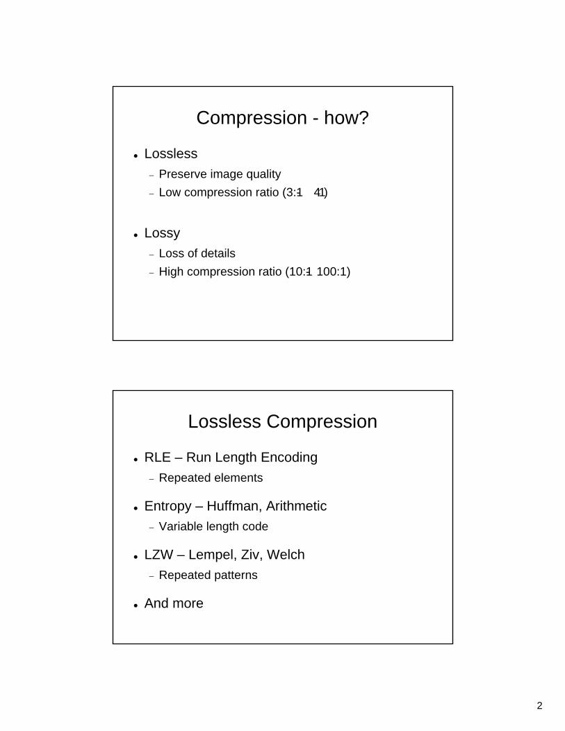
Compression - how?

Lossless− Preserve image quality− Low compression ratio (3:1- 4:1)

Lossy− Loss of details− High compression ratio (10:1- 100:1)

Lossless Compression

RLE – Run Length Encoding− Repeated elements

Entropy – Huffman, Arithmetic− Variable length code

LZW – Lempel, Ziv, Welch− Repeated patterns

And more

3

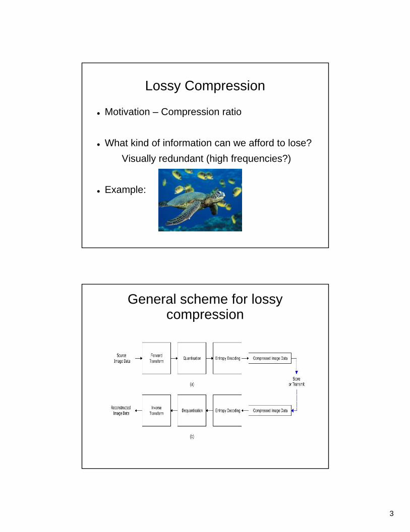
Lossy Compression

Motivation – Compression ratio

What kind of information can we afford to lose?Visually redundant (high frequencies?)

Example:

General scheme for lossy compression

4

Lossy Compression

The most prominent two schemes are:

JPEG – Joint Photographic Expert Group− Extension: .jpg/.jpeg

Wavelets (small waves) – JPEG2000− Extension: .jp2

Both part of DICOM standard(Digital Imaging and Communications in Medicine)

JPEG

DCT based (Discrete Cosine Transform) − A close relative of DFT (no complex numbers) − Transforms the data into the frequency domain

Blocks of 8x8− Introduces blocking artifacts

Scheme:

5

JPEG Example:

Quantization table:

Original -128

DC

T

Quantization

JPEG Example:

original

De-quantizatio

n

+128

Inverse DC

T

Original

6

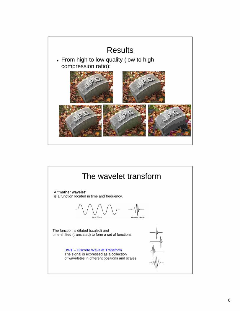
ResultsFrom high to low quality (low to high compression ratio):

The wavelet transform

A “mother wavelet”is a function located in time and frequency.

The function is dilated (scaled) andtime-shifted (translated) to form a set of functions:

DWT – Discrete Wavelet TransformThe signal is expressed as a collectionof waveletes in different positions and scales

7

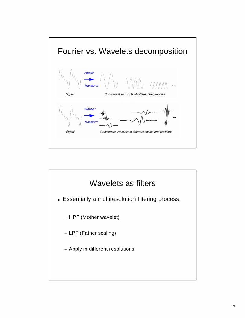
Fourier vs. Wavelets decomposition

Wavelets as filters

Essentially a multiresolution filtering process:

− HPF (Mother wavelet)

− LPF (Father scaling)

− Apply in different resolutions

8

One Stage Filtering Approximations and details:

The low-frequency content is the most important part in many applications, and gives the signal its identity.This part is called “Approximations”

The high-frequency gives the ‘flavor’, and is called “Details”

Approximations and Details:

Approximations:low- frequency components of the signalDetails: high- frequency components

Input Signal

LPF

HPF

A

D

9

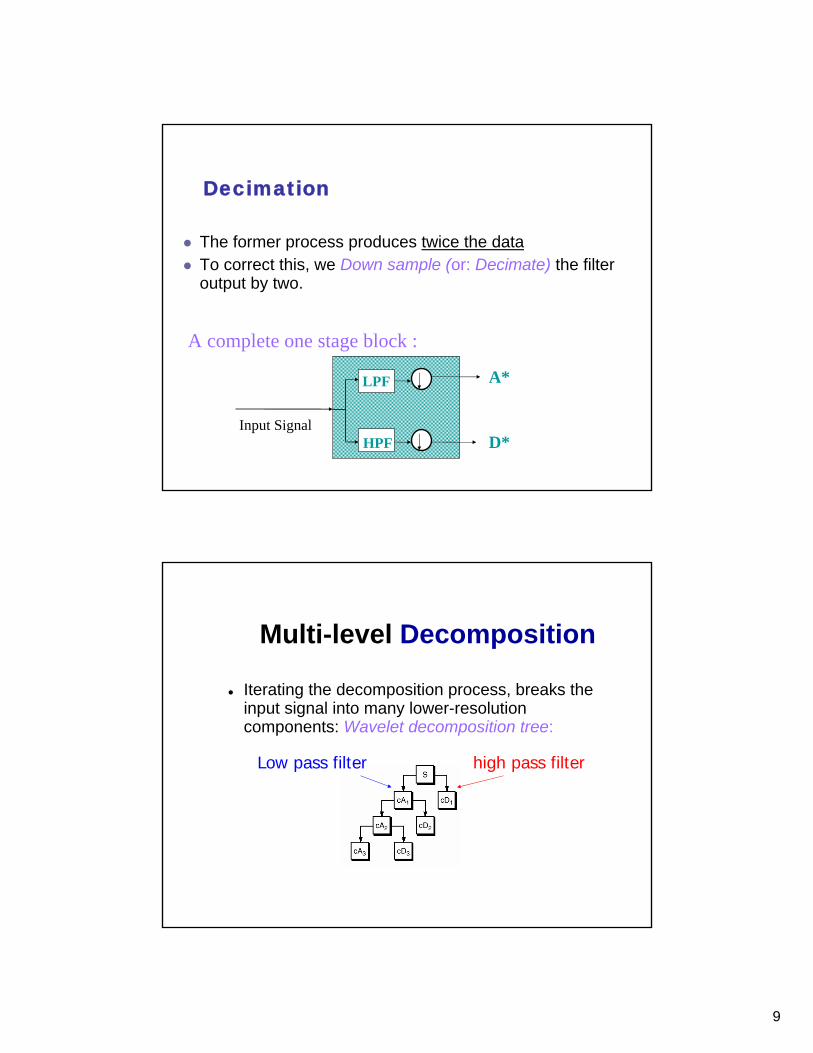
Decimation

The former process produces twice the dataTo correct this, we Down sample (or: Decimate) the filter output by two.

A complete one stage block :

Input Signal

LPF

HPF

A*

D*

Multi-level Decomposition

Iterating the decomposition process, breaks the input signal into many lower-resolution components: Wavelet decomposition tree:

Low pass filter high pass filter

10

A Simple Example: The Haar Wavelet

Consider two neighboring samples a and b of a sequence.- a and b have some correlation.

A simple linear transform:

High correlation- small |d|, fewer bits representation.(i.e. a=b,d=0)

No loss of any information Reconstruction formula of a and b:

The Haar Wavelet Con’t

The key behind Haar Wavelet Transform:these reconstruction formulas can be found by inverting a 2x2 matrix.

11

Sn = {Sn,i | 0=< i <= 2n}

The Haar Wavelet Con’t Signal Sn of 2n sample values Sn,i:

Apply average (Sn-1) and difference (dn-1) transform onto each pair:

a = S2i, b = S2i+1 Sn-1,i = Sn,2i+Sn,2i- 2n-1 pairs (i=0…2n-1) 2

dn-1,i = Sn,2i+1- Sn,2i

Recover the original signal Sn from Sn-1 and dn-1

The Haar Wavelet Con’t Sn-1 as Approximationsdn-1 as Details

Signal with local coherence- approximations closely resembles the

original signal- detail is very small (efficient representation)

12

The Haar Wavelet Con’tApplying the same transform (averages and differences) to Sn-1 itself.Split Sn-1 to (yet) coarser signal Sn-2 and another difference signal dn-2,each of them contain 2n-2

samples.We can repeat this transform n times till S0

contains only one sample S0,0.

This is the Haar transform

The Haar transform

Structure of the wavelet transform: recursively split into averages and differences

Sn

Sn- 1 dn- 1

Sn-2 dn-2

S0 d0

S1 d1

13

The Haar transformd0 d1 dn-2,i dn-1,i

S0 S1 S2 … Sn-1,i Sn,i

Structure of the inverse wavelet transform: recursively merge averages and differences.

The Haar transform Con’t

The cost of computing the transform is O(N).

(FFT cost is O(NlogN))

14

Wavelet functions examples

Haar function

Daubechies function

Coiflet

Symlet

Meyer

Morlet

Biorthogonal Splines

15

Wavelets Image decomposition

One level decomposition

Wavelets Image decomposition

Multi level decomposition

16

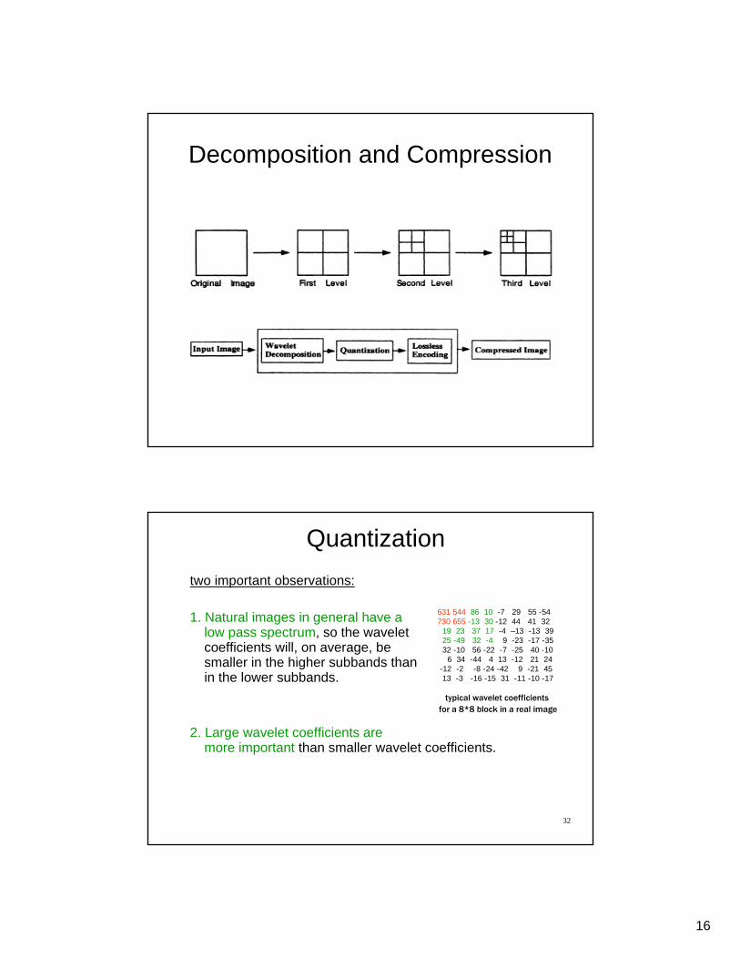
Decomposition and Compression

32

Quantizationtwo important observations:

1. Natural images in general have a low pass spectrum, so the wavelet coefficients will, on average, be smaller in the higher subbands than in the lower subbands.

2. Large wavelet coefficients are more important than smaller wavelet coefficients.

631 544 86 10 -7 29 55 -54 730 655 -13 30 -12 44 41 32

19 23 37 17 -4 –13 -13 39 25 -49 32 -4 9 -23 -17 -35 32 -10 56 -22 -7 -25 40 -10

6 34 -44 4 13 -12 21 24 -12 -2 -8 -24 -42 9 -21 45 13 -3 -16 -15 31 -11 -10 -17

typical wavelet coefficientsfor a 8*8 block in a real image

17

33

Quantization• At low bit rates a large number of the transform

coefficients are quantized to zero (Insignificant Coefficients).

34

Example• Here is a two-stage wavelet decomposition of an image.

Notice the large number of zeros (black):

Matlab toolbox

18

35

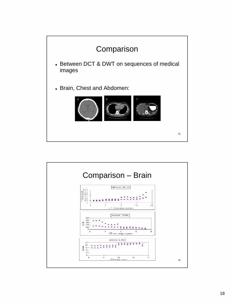
Comparison

Between DCT & DWT on sequences of medical images

Brain, Chest and Abdomen:

36

Comparison – Brain

19

37

Comparison – Chest

38

Comparison – Abdomen

20

39

Comparison

Reconstructed images compressed at 0.25 bpp

JPEG JPEG2000

40

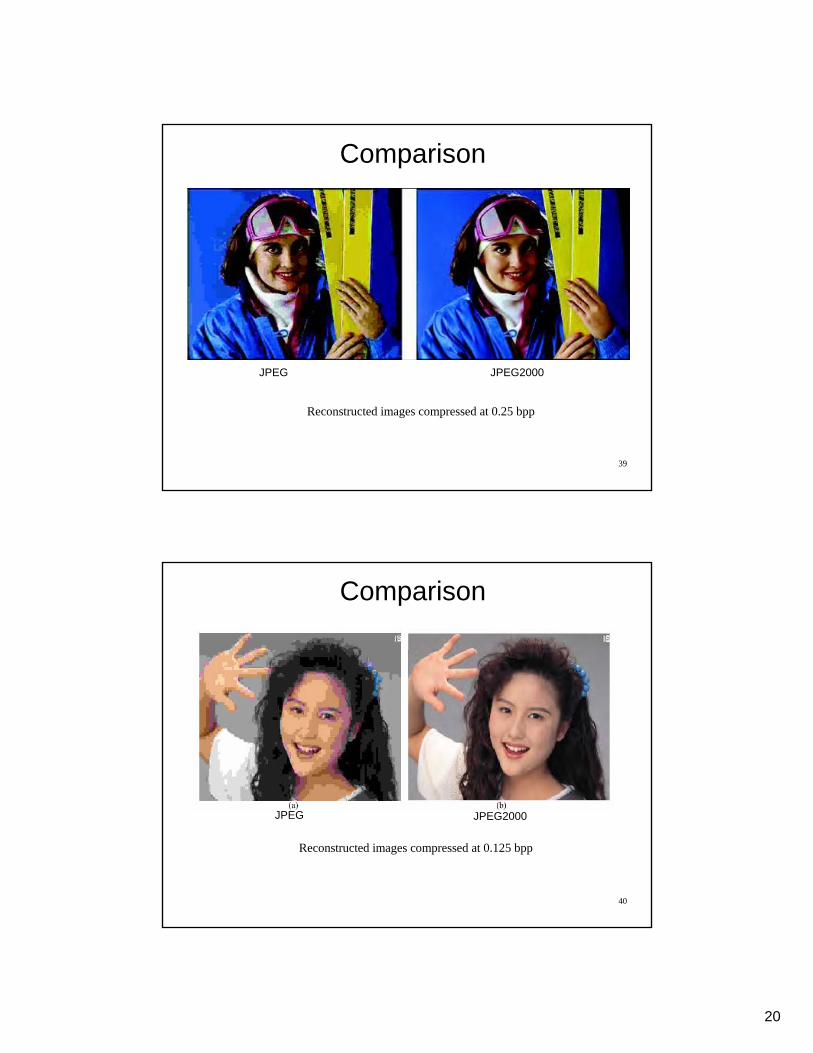
Comparison

Reconstructed images compressed at 0.125 bpp

JPEG2000JPEG

21

41

ComparisonJPEG 2000 (1.83 KB)

Original (979 KB)

JPEG (6.21 KB)

42

Conclusions

DWT outperforms DCT at high compression ratios and is (a bit) fasterDepends on the image – anatomic structures, complexity of diagnostic informationCareful consideration must be given to the level of compression ratio before archiving clinical images otherwise essential information will be lostWavelets in other areas (e.g. epilepsy)