Medical Image Analysis 18 (2014) 359–373

Contents lists available at ScienceDirect

Medical Image Analysis

journal homepage: www.elsevier .com/locate /media

Evaluation of prostate segmentation algorithms for MRI: The PROMISE12challenge

1361-8415/$ - see front matter � 2013 Elsevier B.V. All rights reserved.http://dx.doi.org/10.1016/j.media.2013.12.002

⇑ Corresponding author. Tel.: + 31243655793.E-mail address: g.litjens@rad.umcn.nl (G. Litjens).URL: http://www.diagnijmegen.nl (G. Litjens).

Geert Litjens a,⇑, Robert Toth b, Wendy van de Ven a, Caroline Hoeks a, Sjoerd Kerkstra a,Bram van Ginneken a, Graham Vincent e, Gwenael Guillard e, Neil Birbeck f, Jindang Zhang f,Robin Strand g, Filip Malmberg g, Yangming Ou h, Christos Davatzikos h, Matthias Kirschner i,Florian Jung i, Jing Yuan j, Wu Qiu j, Qinquan Gao k, Philip ‘‘Eddie’’ Edwards k, Bianca Maan l,Ferdinand van der Heijden l, Soumya Ghose d,m,n, Jhimli Mitra d,m,n, Jason Dowling d,Dean Barratt c, Henkjan Huisman a, Anant Madabhushi b

a Radboud University Nijmegen Medical Centre, The Netherlandsb Case Western Reserve University, USAc University College London, England, United Kingdomd Commonwealth Scientific and Industrial Research Organisation, Australiae Imorphics, England, United Kingdomf Siemens Corporate Research, USAg Uppsala University, Swedenh University of Pennsylvania, USAi Technische Universitat Darmstadt, Germanyj Robarts Research Institute, Canadak Imperial College London, England, United Kingdoml University of Twente, The Netherlandsm Université de Bourgogne, Francen Universitat de Girona, Spain

a r t i c l e i n f o

Article history:Received 17 April 2013Received in revised form 3 December 2013Accepted 5 December 2013Available online 25 December 2013

Keywords:SegmentationProstateMRIChallenge

a b s t r a c t

Prostate MRI image segmentation has been an area of intense research due to the increased use of MRI asa modality for the clinical workup of prostate cancer. Segmentation is useful for various tasks, e.g. toaccurately localize prostate boundaries for radiotherapy or to initialize multi-modal registration algo-rithms. In the past, it has been difficult for research groups to evaluate prostate segmentation algorithmson multi-center, multi-vendor and multi-protocol data. Especially because we are dealing with MRimages, image appearance, resolution and the presence of artifacts are affected by differences in scannersand/or protocols, which in turn can have a large influence on algorithm accuracy. The Prostate MR ImageSegmentation (PROMISE12) challenge was setup to allow a fair and meaningful comparison of segmen-tation methods on the basis of performance and robustness. In this work we will discuss the initial resultsof the online PROMISE12 challenge, and the results obtained in the live challenge workshop hosted by theMICCAI2012 conference. In the challenge, 100 prostate MR cases from 4 different centers were included,with differences in scanner manufacturer, field strength and protocol. A total of 11 teams from academicresearch groups and industry participated. Algorithms showed a wide variety in methods and implemen-tation, including active appearance models, atlas registration and level sets. Evaluation was performedusing boundary and volume based metrics which were combined into a single score relating the metricsto human expert performance. The winners of the challenge where the algorithms by teams Imorphicsand ScrAutoProstate, with scores of 85.72 and 84.29 overall. Both algorithms where significantly betterthan all other algorithms in the challenge (p < 0:05) and had an efficient implementation with a run timeof 8 min and 3 s per case respectively. Overall, active appearance model based approaches seemed to out-perform other approaches like multi-atlas registration, both on accuracy and computation time. Although

360 G. Litjens et al. / Medical Image Analysis 18 (2014) 359–373

average algorithm performance was good to excellent and the Imorphics algorithm outperformed thesecond observer on average, we showed that algorithm combination might lead to further improvement,indicating that optimal performance for prostate segmentation is not yet obtained. All results are avail-able online at http://promise12.grand-challenge.org/.

� 2013 Elsevier B.V. All rights reserved.

Table 1Details of the acquisition protocols for the different centers. Each center supplied 25T2-weighted MR images of the prostate.

Center Fieldstrength(T)

Endorectalcoil

Resolution (in-plane/through-plane in mm)

Manufacturer

HK 1.5 Yes 0.625/3.6 SiemensBIDMC 3 Yes 0.25/2.2–3 GEUCL 1.5 and 3 No 0.325–0.625/3–3.6 SiemensRUNMC 3 No 0.5–0.75/3.6–4.0 Siemens

1. Introduction

Prostate MRI image segmentation has been an area of intenseresearch due to the increased use of MRI as a modality for the clin-ical workup of prostate cancer, e.g. diagnosis and treatment plan-ning (Tanimoto et al., 2007; Kitajima et al., 2010; Villeirs et al.,2011; Hambrock et al., 2012; Hoeks et al., 2013). Segmentation isuseful for various tasks: to accurately localize prostate boundariesfor radiotherapy (Pasquier et al., 2007), perform volume estimationto track disease progression (Toth et al., 2011a), to initialize multi-modal registration algorithms (Hu et al., 2012) or to obtain the re-gion of interest for computer-aided detection of prostate cancer(Vos et al., 2012; Tiwari et al., 2013), among others. As manualdelineation of the prostate boundaries is time consuming and sub-ject to inter- and intra-observer variation, several groups have re-searched (semi-) automatic methods for prostate segmentation(Pasquier et al., 2007; Costa et al., 2007; Klein et al., 2008; Makniet al., 2009; Toth et al., 2011b; Chandra et al., 2012; Gao et al.,2012b). However, as most algorithms are evaluated on proprietarydatasets a meaningful comparison is difficult to make.

This problem is aggravated by the fact that most papers cannotinclude a comparison against the state-of-the-art due to previousalgorithms being either closed source or very difficult to imple-ment without help of the original author. Especially in MRI, wheresignal intensity is not standardized and image appearance is for alarge part determined by acquisition protocol, field strength, coilprofile and scanner type, these issues present a major obstacle infurther development and improvement of prostate segmentationalgorithms.

In recent years several successful ‘Grand Challenges in MedicalImaging’ have been organized to solve similar issues in the fields ofliver segmentation on CT (Heimann et al., 2009), coronary imageanalysis (Schaap et al., 2009), brain segmentation on MR (Shattucket al., 2009), retinal image analysis (Niemeijer et al., 2010) and lungregistration on CT (Murphy et al., 2011). The general design ofthese challenges is that a large set of representative training datais publicly released, including a reference standard for the task athand (e.g. liver segmentations). A second set is released to the pub-lic without a reference standard, the test data. The reference stan-dard for the test data is used by the challenge organizers toevaluate the algorithms. Contestants are then allowed to tune theiralgorithms to the training data after which their results on the testdata are submitted to the organizers who calculate predefinedevaluation measures on these test results. The objective of mostchallenges is to provide independent evaluation criteria and subse-quently rank the algorithms based on these criteria. This approachovercomes the usual disadvantages of algorithm comparison, inparticular, bias.

The Prostate MR Image Segmentation (PROMISE12) challengepresented in this paper tries to standardize evaluation and objec-tively compare algorithm performance for the segmentation ofprostate MR images. To achieve this goal a large, representativeset of 100 MR images was made available through the challengewebsite: http://promise12.grand-challenge.org/. This set was sub-divided into training (50), test (30) and live challenge (20) datasets(for further details on the data, see Section 2). Participants coulddownload the data and apply their own algorithms. The goal ofthe challenge was to accurately segment the prostate capsule.

The calculated segmentations on the test set were then submittedto the challenge organizers through the website for independentevaluation. Evaluation of the results included both boundary andvolume based metrics to allow a rigorous assessment of segmenta-tion accuracy. To calculate an algorithm score based on these met-rics, they were compared against human readers. Further detailsabout generation of the algorithm score can be found inSection 3.2.

This paper will describe the setup of the challenge and the ini-tial results obtained prior to and at the workshop hosted by theMICCAI2012 conference in Nice, where a live challenge was heldbetween all participants. New results, which can still be submittedthrough the PROMISE12 website, can be viewed online.

2. Materials

2.1. MRI images

In MRI images, the pixel/voxel intensities and therefore appear-ance characteristics of the prostate can greatly differ betweenacquisition protocols, field strengths and scanners (Dickinsonet al., 2011; Barentsz et al., 2012). Example causes of appearancedifferences include the bias field (Leemput et al., 1999; Sunget al., 2013), signal-to-noise ratio (Fütterer and Barentsz, 2009; Liet al., 2012) and resolution (Tanimoto et al., 2007; Kitajima et al.,2010), especially through-plane. Additionally, signal intensity val-ues are not standardized (Nyúl and Udupa, 1999; Nyúl et al., 2000).Therefore a segmentation algorithm designed for use in clinicalpractice needs to deal with these issues (Bezdek et al., 1993; Clarkeet al., 1993). Consequently, we decided to include data from fourdifferent centers: Haukeland University Hospital (HK) in Norway,the Beth Israel Deaconess Medical Center (BIDMC) in the US, Uni-versity College London (UCL) in the United Kingdom and the Rad-boud University Nijmegen Medical Centre (RUNMC) in theNetherlands. Each of the centers provided 25 transverse T2-weighted MR images. This resulted in a total of 100 MR images.Details pertaining to the acquisition can be found in Table 1. Addi-tionally, a central slice of a data set for each of the centers is shownin Fig. 1 to show the appearance differences. These scans whereacquired either for prostate cancer detection or staging purposes.However, the clinical stage of the patients and the presence andlocation of prostate cancer is unknown to the organizers. Trans-verse T2-weighted MR was used because these contain mostanatomical detail (Barentsz et al., 2012), are used clinically forprostate volume measurements (Hoeks et al., 2013; Toth et al.,2011a) and because most current research papers focus on

Fig. 1. Slice of a data set from different centers to show appearance differences.

G. Litjens et al. / Medical Image Analysis 18 (2014) 359–373 361

segmentation on T2-weighted MRI. The data were then split ran-domly into 50 training cases, 30 test cases and 20 live challengecases. Although the selection process was random, it was stratifiedaccording to the different centers to make sure no training bias to-wards a certain center could occur.

2.2. Segmentation reference standard

Each center provided a reference segmentation of the prostatecapsule performed by an experienced reader. All annotations wereperformed on a slice-by-slice basis using a contouring tool. Thecontouring tool itself was different for the different institutions,but the way cases were contoured was similar. Contouring wasperformed by annotating spline-connected points in either 3DSlic-er (www.slicer.org) or MeVisLab (www.mevislab.de). The refer-ence segmentations were checked by a second expert, C.H., whohas read more than 1000 prostate MRIs, to make sure they wereconsistent. This expert had no part in the initial segmentation ofthe cases and was asked to correct the segmentation if inconsisten-cies were found. The resulting corrected segmentations were usedas the reference standard segmentation for the challenge. Anexample of a reference segmentation at the base, center and apexof the prostate is shown in Fig. 2.

2.3. Second observer

For both the testing and the live challenge data a relatively inex-perienced nonclinical observer (W.v.d.V, two years of experience

Fig. 2. Example T2-weighted transverse prostate MRI images displaying an apical, centrsecond observer segmentation in red. (For interpretation of the references to colour in t

with prostate MR research) was asked to manually segment theprostate capsule using a contouring tool. The second observer wasblinded to the reference standard to make sure both segmentationswere independent. The second observer segmentations were usedto transform the evaluation metrics into a case score, as will be ex-plained in Section 3.2. An example of a second observer segmenta-tion is shown in Fig. 2.

3. Evaluation

3.1. Metrics

The metrics used in this study are widely used for the evalua-tion of segmentation algorithms:

1. the Dice coefficient (DSC) (Klein et al., 2008; Heimann et al.,2009),

2. the absolute relative volume difference, the percentage of theabsolute difference between the volumes (aRVD) (Heimannet al., 2009),

3. the average boundary distance, the average over the shortestdistances between the boundary points of the volumes (ABD)(Heimann et al., 2009),

4. the 95% Hausdorff distance (95HD) (Chandra et al., 2012).

All evaluation metrics were calculated in 3D. We chose bothboundary and volume metrics to give a more complete view of seg-mentation accuracy, i.e. in radiotherapy boundary based metrics

al and basal slice. The reference standard segmentation is shown in yellow and thehis figure legend, the reader is referred to the web version of this article.)

362 G. Litjens et al. / Medical Image Analysis 18 (2014) 359–373

would be more important, whereas in volumetry the volume met-rics would be more important. In addition to evaluating these met-rics over the entire prostate segmentation, we also calculated themspecifically for the apex and base parts of the prostate, becausethese parts are very important to segment correctly, for examplein radiotherapy and TRUS/MR fusion. Moreover, these are the mostdifficult parts to segment due the large inter-patient variability anddifferences in slice thickness. To determine the apex and base theprostate was divided into three approximately equal parts in theslice dimension (the caudal 1/3 of the prostate volume was consid-ered apex, the cranial 1/3 was considered base). If a prostate had anumber of slices not dividable by 3 (e.g. 14), the prostate would bedivided as 4-6-4 for the base, mid-gland and apex respectively.

The DSC was calculated using:

DðX;YÞ ¼ 2jX \ YjjXj þ jY j ð1Þ

where jXj is the number of voxels in the reference segmentation andjY j is the number of voxels in the algorithm segmentation.

The relative volume difference was calculated as:

RVDðX;YÞ ¼ 100� jXjjYj � 1� �

ð2Þ

and thus the absolute relative volume difference is

aRVDðX;YÞ ¼ jRVDðX;YÞj ð3Þ

Note that although we use the aRVD to measure algorithm perfor-mance (both under- and over-segmentation are equally bad), inthe results we will present the RVD, which makes it possible toidentify if algorithms on average tend to over- or under-segmentthe prostate.

For both the 95th percentile Hausdorff distance and the averageboundary distance we first extract the surfaces of the referencesegmentation and the algorithm segmentation. The regular Haus-dorff distance is then defined as:

HDasymðXs;YsÞ ¼maxx2Xs

miny2Ys

dðx; yÞ� �

ð4Þ

HDðXs;YsÞ ¼max HDasymðXs;YsÞ;HDasymðYs;XsÞ� �

ð5Þ

where Xs and Y s are the sets of surface points of the reference andalgorithm segmentations respectively. The operator d is the Euclid-ean distance operator. As the normal Hausdorff distance is very sen-sitive to outliers we use the 95th percentile of the asymmetricHausdorff distances instead of the maximum.

Finally, the average boundary distance (ABD) is defined as:

ABDðXs; YsÞ ¼1

NXs þ NYs

Xx2Xs

miny2Ys

dðx; yÞ þXy2Ys

minx2Xs

dðy; xÞ !

ð6Þ

3.2. Score

Algorithms were ranked by comparing the resulting evaluationmeasures to the second observer and the reference segmentationin a way similar to Heimann et al. (2009). First, the metrics ofthe second observer segmentations are calculated with respect tothe reference segmentation. Then we average each metric overall cases and define a mapping function:

scoreðxÞ ¼maxðaxþ b;0Þ ð7Þ

This function maps a metric value x to a score between 0 and 100.The equation is solved for a and b by setting a score of 100 to a per-fect metric result, e.g. a DSC of 1.0 and setting a score of 85 to a met-ric result equal to the average metric value of the second observer.This will give us two equations to solve the two unknowns, a and b.

Additionally, a score of zero was set as the minimum because other-wise cases with a very poor or missing segmentation could bias thefinal score of an algorithm too much. As an example, if the secondobserver segmentations have an average DSC of 0.83, a and b are88.24 and 11.76 respectively. As such, if an algorithm obtains aDSC of 0.87 on a case the score will be 88.53. This approach is ap-plied to all metrics. The scores for all metrics were averaged to ob-tain a score per case. Then the average over all cases was used torank the algorithms.

A relatively high reference score of 85 was chosen for the sec-ond observer because her segmentations were in excellent corre-spondence with the reference standard. An even higher scorethan 85 would not be warranted, as the segmentations still containerrors experienced observers would not make. The average metricscores for the second observer are presented in Tables 6 and 7.Comparing these metric scores to scores reported in literature forinter-observer variability we can see that they are at approxi-mately at the same level (Pasquier et al., 2007; Costa et al., 2007;Klein et al., 2008; Makni et al., 2009; Toth et al., 2011b; Chandraet al., 2012; Gao et al., 2012b).

The main reason to use this approach is that it allows us toincorporate completely different, but equally important metricslike average boundary distance and the Dice coefficient. Further-more, in addition to allowing us to rank algorithms, the scoresthemselves are also meaningful, i.e. higher scores actually corre-spond to better segmentations. An alternative approach could havebeen to rank algorithms per metric and average the ranks over allmetrics. However, such an average rank is not necessarily relatedto a segmentation performance: the best ranking algorithm couldstill show poor segmentation results that are much worse thanthe second observer.

4. Methods

This section gives an overview of all the segmentation methodsthat participated in the challenge. A short description for each algo-rithm is given. More detailed descriptions of the algorithms can befound in peer-reviewed papers submitted to the PROMISE12 chal-lenge, available at: http://promise12.grand-challenge.org/Results.Algorithms were categorized as either automatic (no user interac-tion at all), semi-automatic (little user interaction, e.g. setting asingle seed point) or interactive (much user interaction, e.g. paint-ing large parts of the prostate). The algorithm categories andadditional details can be found in Tables 2 and 8. The names insubsection titles are the team names chosen by the participantsand are as such not related to the method themselves. Most namesare either abbreviations of group names or company names. Linksto the websites of the individual groups can also be found on thePROMISE12-website.

4.1. Fully automatic segmentation of the prostate using activeappearance models – Imorphics

Vincent et al. (2012) of Imorphics Ltd. have developed a genericstatistical modeling system designed to minimize any bespokedevelopment needed for different anatomical structures and imagemodalities.

The Imorphics system generates a set of dense anatomical land-marks from manually segmented surfaces using a variant of theMinimum Description Length approach to Groupwise Image Regis-tration (Cootes et al., 2005). The correspondence points and associ-ated images are used to build an Appearance Model. TheAppearance Model is matched to an unseen image using an ActiveAppearance Model (AAM) which optimizes the model parameters

Table 2Overall challenge results. The last three columns contain the scores including standard deviations. These scores are an average of all individual metric scores over all cases, asexplained in Section 3.2. For the live challenge scores with an asterisk, teams had either missing or incomplete segmentations for some cases. Incomplete or failed cases wereassigned a score of 0. The scores of these groups over all completed cases is shown in brackets. The UBUdG team did not participate in the live challenge and as such received azero score.

Rank Team name Type Online Live Average

1 Imorphics Automatic 84:36� 7:11 87:07� 3:36 85:72� 5:902 ScrAutoProstate Automatic 83:49� 5:92 85:08� 3:54 84:29� 5:103 CBA Interactive 80:66� 6:46 81:21� 9:60 80:94� 7:864 Robarts Semi-automatic 77:32� 4:04 80:08� 7:18 78:70� 5:515 Utwente Semi-automatic 75:23� 10:53 80:26� 7:30 77:75� 9:376 Grislies Automatic 77:56� 12:60 74:35� 11:28 75:96� 12:087 ICProstateSeg Automatic 76:06� 9:40 75:74� 8:81� ð84:16� 4:43Þ 75:90� 9:178 DIAG Automatic 73:30� 13:69 77:01� 12:09 75:16� 13:079 SBIA Automatic 78:34� 8:22 61:38� 28:22� ð76:72� 7:44Þ 69:86� 18:9510 Rutgers Automatic 65:97� 13:13 71:77� 11:02 68:87� 12:3211 UBUdG Semi-automatic 70:44� 9:12 00:00� 0:0� 35:22� 9:12– SecondObserver – 85:00� 4:50 85:00� 4:91 85:00� 4:67

G. Litjens et al. / Medical Image Analysis 18 (2014) 359–373 363

to generate an instance which matches the image as closely as pos-sible (Cootes et al., 2001).

Active Appearance Models require an initial estimate of themodel parameters including position, rotation and scale. The sys-tem uses a multi-resolution gridded search method. This is startedat a low image and model resolution with a small number of mea-sured residuals to make it reasonably fast. The results of thesesearches are ranked according to the sum of squares of the resid-ual, and a proportion removed from consideration. The remainingsearch results are used to initialize models at a higher resolution,and so on. Finally, the single best result at the highest resolutiongives the segmentation result.

4.2. Region-specific hierarchical segmentation of MR prostate usingdiscriminative learning – ScrAutoProstate

The segmentation pipeline developed by Birkbeck et al. (2012)addresses the challenges of MR prostate segmentation throughthe use of region-specific hierarchical segmentation with discrim-inative learning.

First, an intensity normalization is used to adjust for global con-trast changes across the images. Images with an endorectal coil arethen further enhanced by flattening the intensity profile on thebright regions near the coil using an automatic application of Pois-son image editing (Pérez et al., 2003).

In the next phase of the pipeline, a statistical model of meshsurface variation learned from training data is aligned to the nor-malized image. The pose parameters of the shape model are ex-tracted through the use of marginal space learning (Zheng et al.,2009), which decomposes the estimation of pose into sequentialestimates of the position, orientation, scale, and then the firstfew modes of variation. The estimation of each set of pose param-eters relies on a probabilistic boosting tree classifier to discrimina-tively model the relationship between the image data and theunknown parameters being estimated. During training, each classi-fier automatically selects the most salient features from a large fea-ture pool of Haar and steerable features. After the statistical meshmodel has been aligned to the input image using marginal spacelearning, the segmentation is refined through a coarse-to-fineboundary refinement that uses surface varying classifiers to dis-criminate the boundary of the prostate from adjacent soft tissue.The mesh from this final refinement stage is constrained by thestatistical shape model.

4.3. Smart paint – CBA

Malmberg et al. (2012) have developed an interactive segmen-tation tool called Smart Paint. The user segments the organ of

interest by sweeping the mouse cursor in the object or background,similar to how an airbrush is used. Areas are painted with a semi-transparent color which gives immediate feedback in the choseninteraction plane. As the paint is applied in 3D, when the usermoves to another plane using the mouse thumb-wheel the effectof the painting is seen also there.

The algorithm works by taking both the spatial distance to thecursor and the image content (intensity values) into account. Theimage I and the segmentation function f are mappings from ele-ments of a three dimensional voxel set to the interval [0, 1]. A voxelx belongs to the foreground if f ðxÞP 0:5, and to the backgroundotherwise. Initially, f ¼ 0. The brush tool has a value v that is either1 (to increase the foreground) or 0 (to increase the background). Asingle brush stroke centered at voxel x affects the segmentation atall nearby voxels y according to

f ðyÞ ð1� aðx; yÞÞf ðyÞ þ aðx; yÞv ð8Þ

aðx; yÞ ¼ bð1� jIðyÞ � IðxÞjÞk maxðr � dðx; yÞÞ

r;0

� �ð9Þ

where dðx; yÞ is the Euclidean distance between the voxel centers ofx and y; r is the brush radius specified by the user and b and k areconstants.

Additionally, the user can smooth the current segmentationusing a weighted average filter. The algorithm is not very sensitiveto the values selected for the b and k constants. Values for b were inthe range 0.01–0.1 and for k in the range 1–5 and influence thebehavior of the brush. These variables could be changed by theuser.

4.4. Multi-atlas segmentation of the prostate: a zooming process withrobust registration and atlas selection – SBIA

The multi-atlas based segmentation framework designed by Ouet al. (2012) automatically segments the prostate in MR images. At-lases from 50 training subjects are nonrigidly registered to the tar-get image. The calculated deformations are used to warp expertannotated prostate segmentations of the atlases into the target im-age space. The warped prostate annotations are then fused by theSTAPLE strategy (Warfield et al., 2004) to form a single prostatesegmentation in the target image.

The main challenge in this multi-atlas segmentation frameworkis image registration. To account for the registration challenges,three measures are taken in the multi-atlas segmentation frame-work. First, the DRAMMS image registration algorithm is used(Ou et al., 2010). DRAMMS establishes anatomical correspondencesby using high dimensional texture features at each voxel. Voxeltexture features are more distinct than just using intensity, which

364 G. Litjens et al. / Medical Image Analysis 18 (2014) 359–373

helps to improve registration accuracy. Second, a two-phase strat-egy is used. In phase 1 the entire prostate images from trainingsubjects are used to compute an initial segmentation of the pros-tate in target image. Phase 2 focuses only on the initially seg-mented prostate region and its immediate neighborhood. Third,in each phase, atlas selection is used. Those atlases having highsimilarity with the target image in the prostate regions after regis-tration are kept. Similarity is measured using the correlation coef-ficient, mutual information, as well as the DSC between the warpedprostate annotation and the tentative prostate segmentation.

4.5. Automatic prostate segmentation in MR images with aprobabilistic active shape model – Grislies

Kirschner et al. (2012) segment the prostate with an ActiveShape Model (ASM) (Cootes et al., 2001). For training the ASM,meshes were extracted from the ground truth segmentations usingMarching Cubes (Lorensen and Cline, 1987). Correspondence be-tween the meshes was determined using a nonrigid mesh registra-tion algorithm. The final ASM has 2000 landmarks and was trainedusing principal component analysis (PCA). The actual segmentationis done with a three step approach, consisting of (1) image prepro-cessing, (2) prostate localization and (3) adaption of the ASM to theimage.

In the preprocessing step, the bias field is removed using coher-ent local intensity clustering, and the image intensities are normal-ized (Li et al., 2009). Prostate localization is done using the slidingwindow approach: a boosted classifier based on 3D Haar-like fea-tures is used to decide whether the subimage under the currentdetector window position contains the prostate or not. This ap-proach is similar to the Viola-Jones algorithm for face detectionin 2D images (Viola and Jones, 2001),.

The actual segmentation is done with a Probabilistic ASM. Inthis flexible ASM variant, shape constraints are imposed by mini-mizing an energy term which determines a compromise betweenthree forces: an image energy that draws the model towards de-tected image features, a global shape energy that enforces plausi-bility of the shapes with respect to the learned ASM, and a localshape energy that ensures that the segmentation is smooth. Fordetection of the prostate’s boundary, a boosted detector using 1DHaar-like features is used, which classifies sampled intensity pro-files into boundary and nonboundary profiles.

4.6. An efficient convex optimization approach to 3D prostate MRIsegmentation with generic star shape prior – Robarts

The work by Yuan et al. (2012) proposes a global optimization-based contour evolution approach for the segmentation of 3D pros-tate MRI images, which incorporates histogram matching and avariational formulation of a generic star shape prior.

The proposed method overcomes the existing challenges of seg-menting 3D prostate MRIs: heterogeneous intensity distributionsand a wide variety of prostate shape appearances. The proposedstar shape prior does not stick to any particular object shape fromlearning or specified parameterized models, but potentially re-duces ambiguity of prostate segmentation by ruling out inconsis-tent segments; it provides robustness to the segmentation whenthe image suffers from poor quality, noise, and artifacts.

In addition, a novel convex relaxation based method is intro-duced to evolve a contour to its globally optimal position duringeach discrete time frame, which provides a fully time implicitscheme to contour evolution and allows a large time step size toaccelerate the speed of convergence.

Moreover, a new continuous max-flow formulation is proposed,which is dual to the studied convex relaxation formulation and de-rives a new efficient algorithm to obtain the global optimality of

contour evolution. The continuous max-flow based algorithm isimplemented on GPUs to significantly speed up computation inpractice.

4.7. An automatic multi-atlas based prostate segmentation using localappearance specific atlases and patch-based voxel weighting –ICProstateSeg

Gao et al. (2012a) present a fully automated segmentation pipe-line for multi-center and multi-vendor MRI prostate segmentationusing a multi-atlas approach with local appearance specific voxelweighting.

An initial denoising and intensity inhomogeneity correction isperformed on all images. Atlases are classified into two categories:normal MRI scans An and scans taken with a transrectal coil Am.This is easily achieved by examining the intensity variation aroundthe rectum since the transrectal coil produces significant physicaldistortion but also has a characteristic bright appearance in the lo-cal region near the coil itself. The subatlas database whose atlasappearance is closest to the new target is chosen as the initial atlasdatabase. After that, the top N similar atlases are further chosen foratlas registration by measuring intensity difference in the region ofinterest around prostate.

After all the selected atlases are nonrigidly registered to a targetimage, the resulting transformation is used to propagate the ana-tomical structure labels of the atlas into the space of the target im-age. Finally, a patch-based local voxel weighting strategy isintroduced, which was recently proposed for use in patch-basedbrain segmentation (Coupé et al., 2011) and improved by introduc-ing the weight of the mapping agreement from atlas to target. Afterthat, the label that the majority of all warped labels predict foreach voxel is used for the final segmentation of the target image.

4.8. Prostate MR image segmentation using 3D active appearancemodels – Utwente

The segmentation method proposed by Maan and van derHeijden (2012) is an adaptation of the work presented by Kroonet al. (2012) by using a Shape Context based nonrigid surface reg-istration in combination with 3D Active Appearance Models(AAM).

The first step in AAM training is describing the prostate surfacein each training case by a set of landmarks. Every landmark in atraining case must have a corresponding landmark in all othertraining cases. To obtain the corresponding points Shape Contextbased nonrigid registration of the binary segmentation surfaceswas used (Maan and van der Heijden, 2012; Kroon et al., 2012).PCA is applied to determine the principal modes of the shape var-iation. The appearance model can be obtained in a similar way:first each training image is warped so that its points correspondto the mean shape points. Subsequently, the grey-level informationof the region covered by the mean shape is sampled. After normal-ization, a PCA is applied to obtain the appearance model. The com-bined shape and appearance model can generalize to almost anyvalid example.

During the test phase, the AAM is optimized by minimizing thedifference between the test image and the synthesized images. Themean model is initialized by manually selecting the center of theprostate based on visual inspection. Subsequently, the AAM is ap-plied using two resolutions with both 15 iterations.

4.9. A multi-atlas approach for prostate segmentation in MR images –DIAG

Litjens et al. (2012) investigated the use of a multi-atlassegmentation method to segment the prostate using the Elastix

G. Litjens et al. / Medical Image Analysis 18 (2014) 359–373 365

registration package. The method is largely based on the work ofKlein et al. (2008) and Langerak et al. (2010). The 50 availabletraining data sets are used as atlases and registered to the unseenimage using localized mutual information as a metric. Localizedmutual information calculates the sum of the mutual informationof image patches instead of the mutual information of the entireimage. This approach reduces the effect of magnetic field biasand coil profile on the image registration.

The registration process consists of two steps: first a rough ini-tial alignment is found, after which an elastic registration is per-formed. The 50 registered atlases are then merged to form asignal binary segmentation using the SIMPLE optimization algo-rithm (Langerak et al., 2010). SIMPLE tries to automatically discardbadly registered atlases in an iterative fashion using the correspon-dence of the atlas to the segmentation result in the previous itera-tion. The DSC was used as the evaluation measure in the SIMPLEalgorithm.

4.10. Deformable landmark-free active appearance models:application to segmentation of multi-institutional prostate MRI data –Rutgers

Toth and Madabhushi (2012a) propose a Multi-Feature, Land-mark-Free Active Appearance Model (MFA) based segmentationalgorithm, based on (Toth and Madabhushi, 2012b). The MFA con-tains both a training module and a segmentation module. The MFAis constructed by first aligning all the training images using an af-fine transformation. Second, the shape is estimated by taking thesigned distance to the prostate surface for each voxel, which repre-sents a levelset, such that a value of 0 corresponds to the voxels onthe prostate surface. Third, principal component analysis is used tomap the shape and intensity characteristics of the set of trainingimages to a lower dimensional space. Then a second PCA is per-formed on the joint set of lower dimensional shape and appearancevectors to link the shape and appearance characteristics.

To segment an unseen image, the image must be registered tothe MFA, resulting in transformation T mapping the input imageto the MFA. This is performed by first calculating the PCA projec-tion of the intensities learned from the training data. Then thelinked projections are reconstructed and subsequently the intensi-ties and shape. The normalized cross-correlation between thereconstruction and the original image are calculated and the trans-form T is optimized to obtain maximum normalized cross-correla-tion. The shape corresponding to the optimal transformation wasthresholded at 0 to yield the final segmentation.

While the original algorithm (Toth and Madabhushi, 2012b) de-fined ‘‘T’’ as an affine transformation, to account for the high vari-ability in the prostate shape and appearance (e.g. with or withoutan endorectal coil), a deformable, b-spline based transform wasused to define ‘‘T’’. This resulted in a more accurate registrationthan affine, although further studies suggest that separate subpop-ulation based models could potentially yield more accurate seg-mentations, given enough training data.

4.11. A random forest based classification approach to prostatesegmentation in MRI – UBUdG

The method proposed by Ghose et al. (2012) has two majorcomponents: a probabilistic classification of the prostate and thepropagation of region based levelsets to achieve a binary segmen-tation. The classification problem is addressed by supervised ran-dom decision forest.

During training, the number of slices in a volume containing theprostate is divided into three equal parts as apex, central and baseregions. The individual slices are resized to a resolution of256 � 256 pixels and a contrast-limited adaptive histogram

equalization is performed to minimize the effect of magnetic fieldbias. Each feature vector is composed of the spatial position of apixel and the mean and standard deviation of the gray levels ofits 3 � 3 neighborhood. Three separate decision forests are builtcorresponding to the three different regions of the prostate theapex, the central region and the base. Only 50% of the availabletraining data was used for each of the regions.

During testing the first and the last slices of the prostate are se-lected and the test dataset is divided into the apex, the central andthe base regions. Consecutively preprocessing is done on in thesame way as for the training images. Decision forests trained foreach of the regions are applied to achieve a probabilistic classifica-tion of the apex, the central and the base slices. Finally evolution ofthe Chan and Vese levelsets on the soft classification ensures seg-mentation of the image into prostate and the background regions.

4.12. Combinations of algorithms

It is well known that combining the results of multiple humanobservers often leads to a better segmentation than using the seg-mentation of only a single observer (Warfield et al., 2004). Toinvestigate whether this is also true for segmentation algorithms,different types of combinations were tried. First, combining allthe algorithm results using a majority voting approach was ex-plored. The majority voting combination considered a voxel partof the prostate segmentation if the majority of the algorithms seg-mented the voxel as a prostate voxel. Second, only the top 5 (ex-pert) algorithms were combined based on the overall algorithmscore. A ‘best combination’ reference was also included by select-ing the algorithm with the maximum score per case, for both thetop 5 and all algorithms.

5. Results

5.1. Online challenge

The results of the online challenge are summarized in Tables 2,6 and Fig. 3. In Table 2 the average algorithm scores and standarddeviations are presented, which are used to rank the algorithms.The ordering of the algorithms represents the ranking after boththe online and live challenges. The online and live componentswere weighted equally to determine the final ranking. Metric val-ues and scores for all algorithms on the online challenge data arepresented in Table 6. In Fig. 3 we provide the results per algorithmper case to give a more complete view of algorithm robustness andvariability.

5.2. Live challenge

Tables 2, 7 and Fig. 4 show the results of the live challenge atthe MICCAI2012 workshop. In Table 2 (column 2) the averagescores for each algorithm are presented including standard devia-tions. Metric values and scores for all algorithms on the live chal-lenge data are presented in 7. Fig. 4 shows the scores per caseper algorithm for the cases processed at the live challenge. Algo-rithms that were unable to segment all cases during the periodof the challenge (4 h), or produced segmentations that were con-sidered to be a failure according to algorithm-specific checking cri-teria or the group, are indicated with an asterisk in Table 2.Unsegmented or failed cases were given a score of 0.

5.3. Overall

The overall ranking of the algorithms is presented in Table 2.Additionally, the results of the algorithm combinations are shown

Fig. 3. Results of the online challenge. The overall score is on the vertical axis and the case number on the horizontal axis. Teams are given a different symbol and color. Casedistributions per center were: 1:7 RUNMC, 8:14 BIDMC, 15:22 UCL, 23:30 HK. (For interpretation of the references to colour in this figure legend, the reader is referred to theweb version of this article.)

Fig. 4. Results of the live challenge. The overall score is on the vertical axis and the case number on the horizontal axis. Teams are given a different symbol and color. Casedistributions per center were: 1:5 UCL, 6:10 HK, 11:15 BIDMC, 16:20 RUNMC. (For interpretation of the references to colour in this figure legend, the reader is referred to theweb version of this article.)

Table 3Results for the single best algorithm and combinations of algorithms, average over allcases including standard deviation.

Name Online Live Average

Imorphics 84:36� 7:11 87:07� 3:36 85:72� 5:90All combined 82:96� 8:25 87:70� 3:11 85:33� 6:68Top 5 combined 85:38� 6:13 87:09� 3:22 86:24� 5:16Maximum 87:57� 3:37 88:88� 1:73 88:23� 2:83

366 G. Litjens et al. / Medical Image Analysis 18 (2014) 359–373

in Table 3. Furthermore, statistical analysis on the complete set ofcase scores was also performed to determine which algorithms aresignificantly better than other algorithms. As a test repeated mea-sures ANOVA was used in combination with Bonferroni correctionat a significance level of 0.05. The results indicated that the top 2algorithms by Imorphics and ScrAutoProstate are significantly bet-ter then every algorithm outside of the top 3. This also holds forboth combination strategies. However, none of the algorithms orcombinations strategies performed significantly better than thesecond observer. Finally, the robustness of the algorithms againstmulti-center data was also tested using ANOVA, but the centerdid not have a significant impact on the overall algorithm score(p = 0.118). The average scores and standard deviations for thealgorithms on a per-center basis are presented in Tables 4 and 5.

6. Discussion

6.1. Challenge setup and participation

The images used in the challenge are a good representation ofwhat would be encountered in a clinical setting, with largedifferences in acquisition protocol, prostate appearance and size.

Additionally, the images originated from different centers andscanner manufacturers. The training and test sets were also largeenough to draw statistical conclusions on algorithm performance.

The reference standard was constructed by 3 different observ-ers, who each segmented a part of the data. These segmentationswere subsequently inspected by the experienced observer for cor-rectness and consistency. Obtaining additional observers for eachcase would be preferable, however recruiting multiple observersto spend time contouring 100 prostate MR cases is extremelychallenging.

The metrics that were used result in a good separation betweenalgorithms and the conversion into per case scores keeps these dif-ferences intact. Other metrics were also considered, for examplethe Jaccard index, sensitivity/specificity and regular Hausdorff dis-tance. Jaccard index is a volume-based metric with similar charac-teristics as the Dice coefficient, however, in prostate segmentationliterature, the Dice coefficient is more often used. To allow bettercomparison to existing and future literature we chose the Dicecoefficient. Sensitivity and specificity are generally not useful inprostate segmentation because specificity will not be very discrim-inative: the prostate is always a relative small part of the total im-age volume. Finally, the modified 95% Hausdorff distance was usedbecause the regular Hausdorff distance can be harsh and sensitiveto noise: a single pixel can determine overall image segmentationoutcome.

One issue with basing case scores on observer reference stan-dards is that very high scores end up in the realm of inter-observervariability. A score higher than 85 is probably still indicative of im-proved performance, as the second observer segmentations are lessaccurate than the reference standard, but it is difficult to saywhether a score of e.g. 94 is indeed better or just different andequally accurate than a score of 92. However, in general, the algo-

Fig. 5. Qualitative segmentation results of case 3 (a, b, c), case 10 (d, e, f) and case 25 (g, h, i) at the center (a, d, g), apex (b, e, h) and base (c, f, i) of the prostate. Case 3 had thebest, case 10 reasonable and case 25 the worst algorithm scores on average. The different colors indicate the results for the different teams. (For interpretation of thereferences to colour in this figure legend, the reader is referred to the web version of this article.)

G. Litjens et al. / Medical Image Analysis 18 (2014) 359–373 367

rithms in this challenge do not obtain these scores on average, sothis is not an issue. Visual inspection of the segmentation resultsalso confirms this, the largest segmentation errors made by thealgorithms would not be made by an experienced observer.

An alternative scoring approach that is not sensitive to inter-observer variability is to rank algorithms based on their averagerank for each of the sub-scores over all algorithms (e.g. if analgorithm has the highest average Dice of all algorithms, it willhave rank 1 for Dice. If the same algorithm has rank 5 for averageboundary distance over all algorithms, his average total rankwould be 3). This approach has its own disadvantage, e.g. highranks do not mean good segmentations and algorithm ranking isnot only based on the performance of the algorithm itself, but alsoon the results of other algorithms, i.e. a new algorithm which doesvery poorly on all metrics except one might influence the rankingof all other algorithms by changing their average rank.

Participation in the initial phase of the challenge was similar towhat we have seen in other segmentation challenges, for example(Heimann et al., 2009) and the knee cartilage segmentation chal-lenge (SKI10, http://www.ski10.org). The literature on prostatesegmentation is well represented by the competing algorithms,which include active shape models, atlas-based methods, patternrecognition algorithms and variants.

We specifically chose to allow only single submissions per algo-rithm instead of allowing each group to submit results with differ-ent parameter settings, to make sure there would be ‘no trainingon the test set’.

6.2. Challenge results

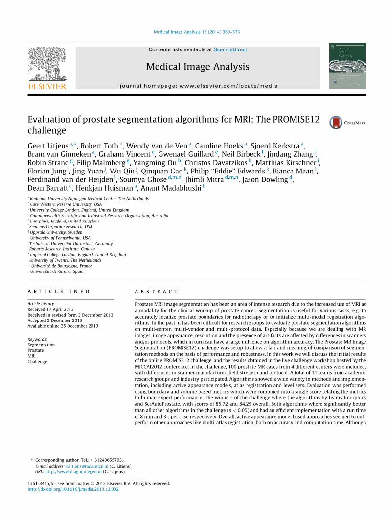
All algorithms submitted to the challenge produced reasonableto excellent results on average (online and live challenge combined

368 G. Litjens et al. / Medical Image Analysis 18 (2014) 359–373

scores ranging from 68.97 to 85.72). One point to note is thatalthough some algorithms may have received the same averagescore, the variability can differ substantially, as shown in Tables6, 7 and 2. For example, the algorithm presented by Robarts (Yuanet al., 2012) scored 77.32 and 80.08 in the online and live challengerespectively, but has a very low variability: 5.51 score standarddeviation overall. This is much lower than the algorithms thathad similar scores, for Example 7.86 for CBA (Malmberg et al.,2012) and 9.37 for Utwente (Maan and van der Heijden, 2012).Depending on the purpose for which an algorithm is used in theclinic, this can be a very important aspect. As such, it might begood to incorporate performance variability directly in algorithmranking in future challenges.

It is worth noting that the top 2 algorithms by Imorphics(Vincent et al., 2012) and ScrAutoProstate (Birkbeck et al., 2012)were completely automatic and even outperformed the completelyinteractive method presented by CBA. Whereas the algorithm byImorphics performed best overall, the algorithm by ScrAutoPro-state should be noted for its exceptionally fast segmentation speed(2.3 s, Table 8), the fastest of all algorithms. Further details aboutinteraction, implementation details and computation time can befound in Table 8. Algorithm computation times varied, with the ac-tive shape model based approaches often having computationtimes in the order of minutes, whereas the atlas based approachesrequired substantially more time or computing power (e.g. clus-ters, GPU). It is important to note that some algorithms wereimplemented in high-level programming languages like Matlab,whereas some where implemented in low-level languages likeC++, computation time is thus not only dependent on algorithmefficiency but also on the development platform.

Inspecting the illustrative results in Fig. 5 one can see that algo-rithms can differ quite substantially per case. In this figure wepresent the best, worst and a reasonable case with respect to

Table 4Average scores and standard deviations per team over the different centers for the online

RUNMC BIDMC

Imorphics 82.55 � 8.72 89.05 �ScrAutoProstate 85.76 � 3.56 86.26 �CBA 76.05 � 7.71 80.82 �Robarts 77.38 � 4.73 76.34 �Utwente 72.52 � 10.27 78.85 �Grislies 81.10 � 9.69 86.10 �ICProstateSeg 72.70 � 10.58 82.12 �DIAG 66.60 � 13.25 77.48 �SBIA 81.02 � 8.77 77.04 �Rutgers 63.98 � 14.82 67.00 �UBUdG 73.17 � 2.88 67.52 �Average 75.69 � 8.63 78.96 �

Table 5Average scores and standard deviations per team over the different centers for the live challincluded here.

RUNMC BIDMC

Imorphics 86.86 � 3.39 88.54 �ScrAutoProstate 85.06 � 2.26 85.44 �CBA 81.32 � 8.52 83.11 �Robarts 81.29 � 5.27 74.77 �Utwente 80.42 � 5.48 79.46 �Grislies 79.98 � 6.64 77.91 �ICProstateSeg 82.75 � 4.67 86.36 �RUNMC 61.77 � 15.90 81.51 �SBIA 79.03 � 7.21 13.57 �Rutgers 72.39 � 14.09 75.10 �Average 79.09 � 7.34 74.58 �

average algorithm performance. Case 25 was especially tricky asit had a large area of fat around the prostate, especially near thebase which appears very similar to prostate peripheral zone. Mostalgorithms oversegmented the prostatic fat, and as the prostatewas relatively small, this results in large volumetric errors.However, if one inspects case 25 carefully, it is possible to makethe distinction between fat and prostate, especially if you gothrough the different slices. It is thus no surprise that the interac-tive segmentation technique of CBA performed the best. Furtherinspection of the results shows that in the cases with low averagealgorithm performance the interactive method is usually the bestalgorithm (e.g. Fig. 3: cases 4, 16 and 21 of the online challenge).This indicates that these cases cause problems for automatedmethods.

In this challenge we explicitly included segmentation results atthe base and the apex of the prostate into the algorithm scoring be-cause these areas are usually the most difficult to segment. Thiscan also be observed in the results, especially Tables 6 and 7. Everyalgorithm performed worse on the apex and base if we look at themetric values (especially the Dice coefficient and the relative vol-ume difference) themselves; however, as these areas are also themost difficult for the human observer, the scores for apex and basetend to be higher than the overall score. Interesting to note is thatthe top 2 algorithms outperform the second observer at almostevery metric for both apex and base, whereas the overall score islower than the second observer. For the live challenge the Imorph-ics algorithm even outperforms the second observer in the overallscore. This indicates that for this part of the prostate automaticalgorithms might improve over human observers.

Interestingly, similar to the SLIVER07-challenge, active shapebased algorithms seemed to give the best results (places 1, 2, 4and 5), although two of these systems are semi-automatic. Lookingat the results in more detail, we can see that the atlas based

challenge.

UCL HK

2.29 84.78 � 7.52 81.44 � 7.413.73 83.12 � 4.95 79.47 � 8.466.37 83.16 � 6.17 82.06 � 4.945.13 77.57 � 3.55 77.88 � 3.778.11 76.50 � 13.02 73.16 � 11.466.35 77.99 � 14.82 66.54 � 10.994.71 77.37 � 7.49 72.40 � 11.925.09 81.45 � 6.76 67.51 � 20.1510.41 77.31 � 7.32 78.15 � 8.1911.99 69.98 � 11.02 62.79 � 16.4614.90 74.31 � 6.39 66.73 � 8.337.19 78.50 � 8.09 73.47 � 10.19

enge. Note that team UBUdG did not participate in the live challenge and as such is not

UCL HK

4.17 86.96 � 3.22 85.92 � 3.593.03 86.39 � 3.67 83.44 � 5.447.88 77.86 � 16.87 82.53 � 4.5911.76 81.96 � 3.99 82.31 � 5.347.51 80.64 � 10.40 80.50 � 8.4212.30 72.18 � 16.30 67.33 � 7.223.18 85.60 � 1.71 80.25 � 5.836.82 83.16 � 5.35 81.61 � 3.8030.33 75.50 � 10.38 77.41 � 4.398.95 65.45 � 14.78 74.14 � 6.249.59 79.57 � 8.67 79.54 � 5.49

Table 6Averages and standard deviations for all metrics for all teams in the online challenge. Entries indicated with an asterisk had cases with infinite boundary distance measuresremoved from the average, which could occur due to empty base or apex segmentation results.

Team name Average boundary distance

Overall Base Apex Score (Overall) Score (Base) Score (Apex)

Imorphics 2.10 � 0.68 2.18 � 1.14 1.96 � 0.80 82.66 � 5.60 85.20 � 7.75 88.44 � 4.71ScrAutoProstate 2.13 � 0.48 2.23 � 0.70 2.18 � 0.68 82.42 � 3.93 84.87 � 4.73 87.17 � 3.98CBA 2.33 � 0.59 2.60 � 1.47 2.44 � 0.81 80.77 � 4.88 82.31 � 9.96 85.62 � 4.75Robarts 2.65 � 0.37 2.92 � 0.88 3.49 � 0.95 78.09 � 3.06 80.14 � 5.97 79.45 � 5.58Utwente 3.03 � 1.06 3.45 � 1.96 2.68 � 0.98 74.96 � 8.73 76.54 � 13.34 84.20 � 5.79Grislies 2.96 � 1.55 3.19 � 2.00 2.46 � 1.26 75.55 � 12.80 78.35 � 13.59 85.50 � 7.42ICProstateSeg 2.86 � 0.82 3.18 � 1.32 2.89 � 1.05 76.34 � 6.78 78.38 � 9.00 82.99 � 6.21DIAG 3.40 � 1.72 4.23 � 3.06 2.72 � 1.75 71.90 � 14.18 71.29 � 20.81 84.01 � 10.33SBIA 2.85 � 0.72 2.82 � 1.02 2.13 � 0.80 76.47 � 5.94 80.86 � 6.93 87.44 � 4.74Rutgers 4.06 � 1.80 4.82 � 2.64⁄ 3.71 � 1.26⁄ 66.47 � 14.87 63.06 � 23.71 74.68 � 16.56UBUdG 4.26 � 1.58 4.21 � 1.42 4.53 � 1.71 64.84 � 13.09 71.40 � 9.63 73.33 � 10.08All combined 2.06 � 0.78 2.60 � 1.53 2.04 � 0.81 82.96 � 6.46 82.30 � 10.36 87.98 � 4.76Top 5 combined 1.94 � 0.48 2.10 � 0.82 1.77 � 0.62 84.00 � 3.95 85.70 � 5.56 89.57 � 3.63Maximum 1.78 � 0.35 1.82 � 0.52 1.58 � 0.35 85.28 � 2.91 87.66 � 3.51 90.70 � 2.06SecondObserver 1.82 � 0.36 2.21 � 0.80 2.55 � 1.08 85.00 � 2.93 85.00 � 5.42 85.00 � 6.34

95% Hausdorff distance

Imorphics 5.94 � 2.14 5.45 � 2.58 4.73 � 1.68 84.20 � 5.70 86.98 � 6.15 88.84 � 3.97ScrAutoProstate 5.58 � 1.49 5.60 � 2.35 4.93 � 1.38 85.15 � 3.98 86.63 � 5.62 88.37 � 3.25CBA 6.57 � 2.11 6.64 � 4.07 5.75 � 1.91 82.50 � 5.61 84.15 � 9.73 86.43 � 4.52Robarts 6.48 � 1.56 6.83 � 2.26 7.36 � 2.11 82.76 � 4.15 83.70 � 5.39 82.62 � 4.98Utwente 7.32 � 2.44 7.69 � 3.75 5.89 � 1.93 80.52 � 6.48 81.64 � 8.94 86.11 � 4.57Grislies 7.90 � 3.83 7.61 � 4.11 5.82 � 2.82 78.97 � 10.19 81.85 � 9.81 86.26 � 6.65ICProstateSeg 7.20 � 1.96 7.27 � 2.92 6.51 � 2.31 80.84 � 5.21 82.64 � 6.97 84.62 � 5.46DIAG 8.59 � 4.00 9.00 � 4.62 5.91 � 3.68 77.15 � 10.66 78.52 � 11.04 86.05 � 8.69SBIA 7.73 � 2.68 6.99 � 2.25 4.60 � 1.31 79.43 � 7.14 83.32 � 5.37 89.14 � 3.10Rutgers 9.25 � 3.76 9.88 � 4.04⁄ 7.58 � 2.35⁄ 75.37 � 10.00 71.18 � 21.41 78.82 � 16.23Rutgers 9.25 � 3.76 9.88 � 4.04⁄ 7.58 � 2.35⁄ 75.37 � 10.00 71.18 � 21.41 78.82 � 16.23UBUdG 9.17 � 3.48 9.06 � 2.71 9.54 � 3.52 75.59 � 9.27 78.38 � 6.46 77.48 � 8.30All combined 5.43 � 2.18 6.00 � 3.06 4.97 � 1.94 85.55 � 5.81 85.67 � 7.30 88.26 � 4.57Top 5 combined 5.30 � 1.60 5.37 � 2.38 4.22 � 1.25 85.91 � 4.26 87.19 � 5.67 90.04 � 2.94Maximum 4.63 � 1.06 4.32 � 1.28 3.67 � 0.70 87.67 � 2.81 89.68 � 3.05 91.34 � 1.64SecondObserver 5.64 � 1.73 6.28 � 2.95 6.36 � 2.40 85.00 � 4.61 85.00 � 7.04 85.00 � 5.66

Dice coefficient

Imorphics 0.88 � 0.04 0.86 � 0.08 0.85 � 0.08 81.96 � 6.62 84.76 � 8.93 88.57 � 6.13ScrAutoProstate 0.87 � 0.04 0.86 � 0.04 0.83 � 0.07 81.14 � 5.39 85.02 � 4.58 87.79 � 5.23CBA 0.87 � 0.04 0.84 � 0.07 0.80 � 0.11 79.80 � 5.36 82.87 � 8.07 85.46 � 7.98Robarts 0.84 � 0.03 0.81 � 0.05 0.71 � 0.12 75.32 � 4.25 79.77 � 5.82 78.70 � 8.84Utwente 0.82 � 0.07 0.78 � 0.13 0.78 � 0.09 72.97 � 9.77 76.12 � 13.85 84.10 � 6.44Grislies 0.83 � 0.08 0.81 � 0.11 0.82 � 0.10 75.10 � 12.38 79.17 � 11.85 86.65 � 7.09ICProstateSeg 0.82 � 0.06 0.76 � 0.13 0.74 � 0.13 72.68 � 9.40 74.12 � 14.15 80.47 � 9.41DIAG 0.80 � 0.09 0.71 � 0.22 0.79 � 0.12 69.62 � 14.20 68.38 � 23.42 84.82 � 8.77SBIA 0.84 � 0.06 0.81 � 0.08 0.84 � 0.07 75.29 � 8.27 79.29 � 9.07 88.11 � 5.31Rutgers 0.74 � 0.10 0.61 � 0.25 0.66 � 0.17 61.05 � 15.36 57.75 � 25.70 74.93 � 12.60UBUdG 0.71 � 0.11 0.71 � 0.12 0.63 � 0.14 56.73 � 16.09 68.17 � 12.80 72.53 � 10.20All combined 0.88 � 0.05 0.81 � 0.13 0.81 � 0.11 81.29 � 7.55 78.90 � 14.20 86.31 � 8.39Top 5 combined 0.89 � 0.03 0.87 � 0.05 0.87 � 0.06 83.65 � 4.82 85.79 � 5.96 90.32 � 4.63Maximum 0.90 � 0.02 0.89 � 0.03 0.88 � 0.03 85.08 � 3.55 88.20 � 3.80 91.46 � 2.50SecondObserver 0.90 � 0.03 0.86 � 0.06 0.80 � 0.11 85.00 � 3.82 85.00 � 6.14 85.00 � 8.39

Relative volume difference

Imorphics 2.92 � 15.71 1.01 � 19.56 0.65 � 30.68 72.53 � 25.31 84.03 � 16.94 84.20 � 16.97ScrAutoProstate 11.53 � 14.05 9.65 � 16.52 14.08 � 34.25 68.18 � 27.94 82.67 � 14.82 82.52 � 18.44CBA 12.75 � 13.99 18.85 � 24.88 0.41 � 28.63 63.48 � 25.38 72.51 � 24.00 82.04 � 11.91Robarts 10.31 � 17.92 12.69 � 26.26 �3.27 � 39.09 61.70 � 28.63 70.65 � 18.41 74.96 � 15.61Utwente 22.30 � 27.88 27.52 � 41.86 15.10 � 41.30 50.19 � 32.42 57.94 � 31.74 77.45 � 23.46Grislies 19.81 � 31.93 23.12 � 44.71 15.46 � 43.71 59.25 � 38.47 64.73 � 31.20 79.31 � 23.00ICProstateSeg �2.61 � 24.86 �4.47 � 35.14 �13.31 � 43.42 57.96 � 34.16 66.62 � 25.50 75.09 � 20.77DIAG 4.66 � 28.30 �9.34 � 43.13 11.66 � 54.14 51.04 � 31.02 60.62 � 31.86 76.15 � 24.37SBIA 16.19 � 25.35 13.47 � 30.78 11.26 � 35.57 51.63 � 35.95 67.71 � 23.49 81.33 � 21.19Rutgers �5.83 � 30.81 �22.11 � 57.39 �16.68 � 46.37 52.18 � 30.04 44.52 � 31.99 71.58 � 24.00UBUdG �5.16 � 21.40 �7.33 � 28.05 �14.55 � 33.25 59.02 � 24.71 69.96 � 16.63 77.87 � 16.16All combined �10.02 � 14.62 �15.45 � 25.94 �19.44 � 22.45 67.17 � 25.33 73.19 � 23.89 81.67 � 13.00Top 5 combined 7.63 � 13.45 7.32 � 18.53 6.37 � 27.31 73.70 � 25.02 82.15 � 15.60 86.50 � 16.37Maximum 2.76 � 3.05 4.50 � 4.80 4.23 � 4.21 93.48 � 7.19 94.61 � 5.76 96.78 � 3.21SecondObserver �1.87 � 7.32 �6.17 � 13.49 �16.24 � 21.13 85.00 � 9.23 85.00 � 9.23 85.00 � 13.57

G. Litjens et al. / Medical Image Analysis 18 (2014) 359–373 369

systems comparatively have more trouble with cases which are notwell represented by the training set, for example case 23, whichhas a prostate volume of 325 mL, while the average is around50 mL.

One interactive method was included (team CBA) which onaverage scored 80.94, which is considerably lower than the secondobserver. This is mostly caused by over-segmentation at the baseof the prostate, often the seminal vesicles were included in the

Table 7Averages and standard deviations for all metrics for all teams in the live challenge. Entries indicated with an asterisk had cases with infinite boundary distance measures removedfrom the average, which could occur due to empty segmentation results.

Team name Average boundary distance

Overall Base Apex Score (Overall) Score (Base) Score (Apex)

Imorphics 1.95 � 0.36 2.45 � 0.65 1.83 � 0.53 85.53 � 2.70 87.12 � 3.41 88.21 � 3.39ScrAutoProstate 2.18 � 0.36 2.34 � 0.78 2.16 � 0.70 83.86 � 2.65 87.73 � 4.12 86.05 � 4.50CBA 2.56 � 0.96 2.48 � 1.55 119.28 � 522.54 81.03 � 7.10 86.95 � 8.13 80.06 � 21.12Robarts 2.67 � 0.62 2.66 � 0.90 3.93 � 2.42 80.23 � 4.56 86.01 � 4.74 74.64 � 15.57Utwente 2.87 � 0.79 3.47 � 1.33 2.43 � 0.72 78.79 � 5.87 81.76 � 6.96 84.32 � 4.62Grislies 4.17 � 2.35 3.75 � 2.25 2.82 � 1.06 69.14 � 17.43 80.31 � 11.80 81.81 � 6.84ICProstateSeg 2.35 � 0.99 2.62 � 1.37 1.95 � 0.96 82.63 � 7.35 86.23 � 7.21 87.46 � 6.16DIAG 3.21 � 1.39 237.53 � 718.80 2.31 � 0.71 76.26 � 10.29 71.09 � 27.15 85.11 � 4.57SBIA 3.13 � 0.74⁄ 3.13 � 0.64⁄ 2.89 � 1.03⁄ 61.49 � 31.92 66.83 � 34.41 65.10 � 33.91Rutgers 3.84 � 1.37 3.70 � 1.12⁄ 4.21 � 1.83 71.54 � 10.18 72.52 � 25.41 72.87 � 11.80All combined 1.97 � 0.34 2.18 � 0.64 1.82 � 0.53 85.43 � 2.51 88.55 � 3.35 88.28 � 3.41Top 5 combined 1.90 � 0.32 2.15 � 0.80 1.92 � 0.64 85.93 � 2.37 88.70 � 4.18 87.61 � 4.14Maximum 1.87 � 0.30 1.82 � 0.45 1.53 � 0.30 86.17 � 2.20 90.44 � 2.36 90.17 � 1.88SecondObserver 2.03 � 0.50 2.86 � 1.26 2.33 � 1.35 85.00 � 3.73 85.00 � 6.63 85.00 � 8.69

95% Hausdorff distance

Imorphics 5.54 � 1.74 6.09 � 1.61 4.58 � 1.36 86.35 � 4.28 87.96 � 3.19 87.03 � 3.86ScrAutoProstate 6.04 � 1.67 5.64 � 2.17 4.60 � 1.39 85.11 � 4.12 88.84 � 4.29 86.96 � 3.94CBA 7.34 � 3.08 6.29 � 3.03 122.28 � 523.16 81.90 � 7.59 87.55 � 6.00 80.72 � 20.05Robarts 7.15 � 2.08 6.12 � 2.14 7.76 � 3.20 82.38 � 5.12 87.89 � 4.22 78.01 � 9.06Utwente 6.72 � 1.42 7.42 � 2.38 5.68 � 1.66 83.43 � 3.51 85.33 � 4.71 83.91 � 4.70Grislies 11.08 � 5.85 8.68 � 4.61 6.88 � 2.21 72.68 � 14.42 82.83 � 9.11 80.49 � 6.27ICProstateSeg 5.89 � 2.59 5.64 � 2.73 4.58 � 2.35 85.48 � 6.38 88.83 � 5.41 87.00 � 6.67DIAG 7.95 � 3.21 242.13 � 719.85 4.74 � 1.34 80.40 � 7.91 75.30 � 26.69 86.56 � 3.79SBIA 7.07 � 1.64⁄ 7.21 � 1.96⁄ 5.93 � 1.69⁄ 66.05 � 34.07 68.59 � 35.35 66.54 � 34.40Rutgers 8.48 � 2.53 242.00 � 719.42 7.82 � 2.42 79.09 � 6.23 75.29 � 26.10 77.82 � 6.86All combined 5.67 � 1.82 5.14 � 1.40 4.46 � 1.46 86.01 � 4.49 89.84 � 2.78 87.35 � 4.13Top 5 combined 5.49 � 1.54 5.48 � 2.24 4.56 � 1.51 86.45 � 3.80 89.16 � 4.43 87.07 � 4.27Maximum 4.80 � 1.02 4.20 � 0.94 3.53 � 0.76 88.17 � 2.52 91.69 � 1.86 90.13 � 2.10SecondObserver 6.08 � 2.23 7.58 � 3.90 5.29 � 2.53 85.00 � 5.50 85.00 � 7.71 85.00 � 7.17

Dice coefficient

Imorphics 0.89 � 0.03 0.84 � 0.06 0.86 � 0.07 85.51 � 3.92 86.98 � 5.21 89.15 � 5.66ScrAutoProstate 0.87 � 0.03 0.85 � 0.06 0.83 � 0.10 83.17 � 3.53 87.35 � 5.20 86.81 � 7.47CBA 0.85 � 0.08 0.85 � 0.10 0.77 � 0.23 79.69 � 10.77 87.82 � 8.16 82.13 � 17.39Robarts 0.84 � 0.04 0.84 � 0.06 0.67 � 0.22 78.82 � 5.40 86.62 � 4.90 74.31 � 17.27Utwente 0.83 � 0.06 0.77 � 0.10 0.79 � 0.10 77.46 � 7.61 81.40 � 7.81 84.12 � 7.47Grislies 0.77 � 0.12 0.78 � 0.12 0.79 � 0.09 70.04 � 16.09 81.93 � 9.79 83.82 � 7.30ICProstateSeg 0.76 � 0.26 0.72 � 0.26 0.74 � 0.26 71.70 � 25.03 77.24 � 21.30 80.26 � 20.36DIAG 0.80 � 0.07 0.63 � 0.30 0.82 � 0.07 73.81 � 9.43 69.73 � 24.09 86.18 � 5.71SBIA 0.65 � 0.34 0.64 � 0.34 0.63 � 0.33 60.41 � 31.93 70.99 � 27.41 71.78 � 25.83Rutgers 0.75 � 0.10 0.68 � 0.25 0.62 � 0.22 67.41 � 13.75 73.93 � 20.13 70.85 � 17.08All combined 0.89 � 0.03 0.87 � 0.05 0.86 � 0.08 86.10 � 3.30 89.01 � 4.10 88.93 � 5.88Top 5 combined 0.89 � 0.02 0.87 � 0.06 0.85 � 0.09 86.12 � 2.90 89.03 � 4.94 88.21 � 6.58Maximum 0.90 � 0.02 0.89 � 0.03 0.89 � 0.03 86.51 � 2.47 90.97 � 2.82 91.90 � 1.97SecondObserver 0.89 � 0.03 0.82 � 0.10 0.81 � 0.15 85.00 � 4.18 85.00 � 8.32 85.00 � 11.56

Relative volume difference

Imorphics �1.50 � 9.15 �8.31 � 18.08 �1.03 � 23.97 86.31 � 13.01 87.15 � 7.70 87.55 � 10.37ScrAutoProstate 10.05 � 11.56 7.77 � 22.01 9.59 � 30.51 73.96 � 17.56 86.55 � 11.38 84.60 � 15.29CBA 12.26 � 17.73 24.75 � 41.69 �7.05 � 39.63 63.49 � 24.70 81.63 � 24.91 81.50 � 20.08Robarts �1.72 � 17.47 5.30 � 25.52 �29.19 � 37.14 71.84 � 21.87 86.46 � 14.29 73.77 � 18.61Utwente 12.62 � 22.25 20.75 � 37.43 0.66 � 28.70 62.15 � 30.81 75.02 � 20.62 85.40 � 12.77Grislies 43.13 � 65.32 36.41 � 58.73 7.23 � 38.19 37.72 � 40.30 72.42 � 29.35 79.01 � 15.76ICProstateSeg �8.49 � 34.17 �14.15 � 34.88 �14.88 � 36.55 69.10 � 29.32 81.82 � 22.02 80.77 � 18.68DIAG �12.34 � 18.38 �38.10 � 32.87 1.61 � 28.65 64.59 � 25.81 70.54 � 24.65 84.60 � 11.74SBIA 6.55 � 59.45 2.66 � 57.32 12.12 � 68.31 30.65 � 34.34 64.84 � 24.89 62.50 � 28.06Rutgers �14.59 � 26.52 �24.79 � 31.88 �24.37 � 47.01 50.76 � 27.17 76.87 � 20.18 72.31 � 22.95All combined 2.69 � 9.75 �0.16 � 13.09 �2.25 � 24.49 83.77 � 12.66 91.64 � 5.14 87.48 � 10.93Top 5 combined 4.69 � 9.95 6.89 � 20.16 �3.07 � 26.74 82.19 � 13.65 88.57 � 11.35 86.10 � 11.74Maximum 1.80 � 1.43 3.65 � 3.24 3.58 � 3.99 96.28 � 2.94 97.21 � 2.47 97.52 � 2.74SecondObserver �5.72 � 7.44 �17.49 � 18.12 �17.97 � 22.90 85.00 � 12.07 85.00 � 11.93 85.00 � 13.03

370 G. Litjens et al. / Medical Image Analysis 18 (2014) 359–373

prostate segmentation. Thus this algorithm is very dependent onthe operator; in principle the algorithm should be able to get closeto expert performance given an expert reader.

There were several semi-automatic algorithms (teams Robarts,UTwente and UBUdG) which needed manual interaction to initial-ize the algorithms. The interaction types and the influence thisinteraction has on segmentation accuracy will differ between the

algorithms. Although none of the teams have explicitly tested therobustness to different initializations, some general commentscan be made. For the Robarts algorithm a number of points onthe prostate boundary have to be set (8 to 10) to initialize a shapeand the initial foreground and background distributions. As such,the algorithm is robust to misplacing single points. For theUtwente algorithm, the prostate center has to be indicated to

Table 8Details on computation time, interaction and computer systems used for the different algorithms. If algorithms where multi-threaded (MT) or used the GPU this is also indicated.

Team name Avg.time

System MT GPU Availability Remarks

Imorphics 8 min 2.83 GHz4-cores

No No Commercially available (http://www.imorphics.com/).

ScrAutoProstate 2.3 s 2.7GGz12-cores

Yes Notavailable

No

CBA 4 min 2.7 GHz2-cores

No No Binaries available at: http://www.cb.uu.se/filip/SmartPaint/ Fully interactive painting

Robarts 45 s 3.2 GHz1-core,

No Yes Available at http://www.mathworks.com/matlabcentral/fileexchange

User indicates 8 to 10 points on prostatesurface

/34126-fast-continuous-max-flow-algorithm-to-2d3d-image-segmentation

512 CUDA-cores

Utwente 4 min 2.94 GHz4-cores

Yes No Not available User indicates prostate center

Grislies 7 min 2.5 GHz4-cores

No No Not available

ICProstateSeg 30 min 3.2 GHz4-cores,

No Yes Not available

96 CUDA-cores

DIAG 22 min 2.27 GHz8-cores

No No Registration algorithm available on http://elastix.isi.uu.nl/ Runs algorithm on a cluster of 50 cores,

average time without cluster 7 min peratlas

SBIA 40 min 2.9 GHz,2 cores

No No Registration algorithm available on Runs algorithm on a cluster of 140 cores,

http://www.rad.upenn.edu/sbia/software/dramms/ average time without cluster 25 min peratlas

Rutgers 3 min 2.67 GHz,8-cores

Yes No Not available

UBUdG 100 s 3.2 GHz4-cores

No No Not available User selects first and last prostate slice

G. Litjens et al. / Medical Image Analysis 18 (2014) 359–373 371

initialize the active appearance and shape models. Big deviations inpoint selection can cause problems for active appearance andshape models, however in general they are pretty robust againstsmall deviations (Cootes et al., 2001). For the UBUdG method, theuser has to select the first and last slice of the prostate. As such,the algorithm will be unable to segment the prostate if it extendsbeyond those slices, which is an issue if users cannot correctlyidentify the start and end slice of the prostate.

Another aspect which plays a role in this challenge was therobustness of the algorithms to multi-center data. The image dif-ferences between the centers were actually quite large, especiallybetween the endorectal coil and nonendorectal coil cases, as canbe seen in Fig. 1. Differences include coil artifacts near the periph-eral zone, coil profiles, image intensities, slice thickness and reso-lution. However, if we look at for example Tables 4, 5, 7 and 8and Fig. 3, it can be seen that all submitted algorithms are at leastreasonably robust against these differences. We could not find anysignificant differences in the performance of the algorithms rela-tive to the different centers using ANOVA (p = 0.118).

We also investigated whether segmentation performance couldbe improved by making several algorithm combinations. First, amajority voting on the segmentation results of all algorithms andthe top 5 best performing was calculated. Second, to get a referencefor the best possible combination we took the best performingscore per case. The summary results of these combinations canbe found in Table 3. Taking the best results per case results in asubstantially better average score than the best performing algo-rithms. This might be an indication that certain cases might be bet-ter suited to some algorithms, and as such, that algorithm selectionshould be performed on a case-by-case basis. The combinations ofalgorithms using majority voting also shows that given the correctcombination, algorithm results can be improved (84.36 to 85.38 forthe online challenge and 87.07 to 87.70 for the live challenge).

Although the increase in score is small, it is accompanied by areduction of the standard deviation (for the top 5 combinationstrategy, Table 3), as the improvements especially occur in poorperforming cases. These scores and the reduction in standard devi-ation thus show that combining algorithms might result in morerobust segmentation. These scores also show that there still isroom for improvement for the individual algorithms. How to com-bine and which algorithms to combine is a nontrivial problem andwarrants further investigation.

Finally, to assess the statistical significance of differences inalgorithm performance we used repeated measures ANOVA withBonferroni correction. The methods by Imorphics and ScrAutoPro-state perform significantly better than all the algorithms outside ofthe top 3 (p < 0:05).

7. Future work and concluding remarks

Although in general the segmentation algorithms, especially thetop 2, gave good segmentation results, some challenges still re-main. As we could see in case 25 (Fig. 5), algorithms sometimesstruggle with the interface between the prostate and surroundingtissue. This is not only true for peri-prostatic fat, but also for theinterface between the prostate and the rectum, the bladder andthe seminal vesicles. Part of these challenges could be addressedby increasing through-plane resolution, but integration of thesestructures into the segmentation algorithms might also improveperformance. Examples included coupled active appearance mod-els (Cootes et al., 2000) or hierarchical segmentation strategies(Wolz et al., 2012). Furthermore, the enormous volume differencesthat can occur in the prostate can also be problematic: case 23 hada volume which was approximately 6 times as large as the average.Automatically selecting appropriate atlas sets or appearance mod-els based on an initial segmentation could be a solution. In the

372 G. Litjens et al. / Medical Image Analysis 18 (2014) 359–373

difficult cases the interactive segmentation method of team CBAwas often the best. This shows that automated performance couldstill be improved.

Future work on prostate segmentation might also focus on thesegmentation of related prostatic structures or substructures.Examples are segmentation of the prostatic zones (transition, cen-tral and peripheral), the neurovascular bundles or the seminalvesicles.

Solving these remaining issues might lead to algorithms which,for any case, can replace the tedious task of manually outlining byhumans without any intervention. Until we are at that level, thechallenge itself will remain online for new submissions and canthus be used as a reference for algorithm performance on multi-center data. As such it could lead to more transparency in medicalimage analysis.

Acknowledgments

This research was funded by Grant KUN2007-3971 from theDutch Cancer Society and by the National Cancer Institute of theNational Institutes of Health under Award Nos. R01CA136535-01,R01CA140772-01, and R21CA167811-01; the National Institute ofBiomedical Imaging and Bioengineering of the National Institutesof Health under Award No. R43EB015199-01; the National ScienceFoundation under Award No. IIP-1248316; the QED award fromthe University City Science Center and Rutgers University. The con-tent is solely the responsibility of the authors and does not neces-sarily represent the official views of the National Institutes ofHealth.

References

Barentsz, J.O., Richenberg, J., Clements, R., Choyke, P., Verma, S., Villeirs, G.,Rouviere, O., Logager, V., Fütterer, J.J., European Society of Urogenital Radiology,2012. ESUR prostate MR guidelines 2012. Eur. Radiol. 22, 746–757.

Bezdek, J.C., Hall, L.O., Clarke, L.P., 1993. Review of MR image segmentationtechniques using pattern recognition. Med. Phys. 20, 1033–1048.

Birkbeck, N., Zhang, J., Requardt, M., Kiefer, B., Gall, P., Kevin Zhou, S., 2012. Region-specific hierarchical segmentation of MR prostate using discriminative learning.MICCAI Grand Challenge: Prostate MR Image Segmentation 2012.

Chandra, S.S., Dowling, J.A., Shen, K.K., Raniga, P., Pluim, J.P.W., Greer, P.B., Salvado,O., Fripp, J., 2012. Patient specific prostate segmentation in 3-D magneticresonance images. IEEE Trans. Med. Imaging 31, 1955–1964.

Clarke, L.P., Velthuizen, R.P., Phuphanich, S., Schellenberg, J.D., Arrington, J.A.,Silbiger, M., 1993. MRI: stability of three supervised segmentation techniques.Magn. Reson. Imaging 11, 95–106.

Cootes, T.F., Edwards, G.J., Taylor, C.J., 2001. Active appearance models. IEEE Trans.Pattern Anal. Mach. Intell. 23, 681–685.

Cootes, T.F., Twining, C.J., Petrovic, V., Schestowitz, R., Taylor, C.J., 2005. Groupwiseconstruction of appearance models using piece-wise affine deformations. In:Proceedings of 16th British Machine Vision Conference, pp. 879–888.

Cootes, T.F., Walker, K., Taylor, C.J., 2000. View-based active appearance models. In:Proc. 4th IEEE Int. Conf. on Automatic Face and Gesture Recognition. IEEEComput. Soc., pp. 227–232.

Costa, M.J., Delingette, H., Novellas, S., Ayache, N., 2007. Automatic segmentation ofbladder and prostate using coupled 3D deformable models. Med. ImageComput. Comput. Assist. Interv. 10, 252–260.

Coupé, P., Manjón, J.V., Fonov, V., Pruessner, J., Robles, M., Collins, D.L., 2011. Patch-based segmentation using expert priors: application to hippocampus andventricle segmentation. Neuroimage 54, 940–954.

Dickinson, L., Ahmed, H.U., Allen, C., Barentsz, J.O., Carey, B., Fütterer, J.J., Heijmink,S.W., Hoskin, P.J., Kirkham, A., Padhani, A.R., Persad, R., Puech, P., Punwani, S.,Sohaib, A.S., Tombal, B., Villers, A., van der Meulen, J., Emberton, M., 2011.Magnetic resonance imaging for the detection, localisation, and characterisationof prostate cancer: recommendations from a european consensus meeting. Eur.Urol. 59, 477–494.

Fütterer, J.J., Barentsz, J., 2009. 3T MRI of prostate cancer. Appl. Radiol. 38, 25–37.Gao, Q., Rueckert, D., Edwards, P., 2012. An automatic multi-atlas based prostate

segmentation using local appearance-specific atlases and patch-based voxelweighting. MICCAI Grand Challenge: Prostate MR Image Segmentation 2012.

Gao, Y., Liao, S., Shen, D., 2012b. Prostate segmentation by sparse representationbased classification. Med. Phys. 39, 6372–6387.

Ghose, S., Mitra, J., Oliver, A., Martí, R., Lladó, X., Freixenet, J., Vilanova, J.C., Sidibé, D.,Meriaudeau, F., 2012. A random forest based classification approach to prostatesegmentation in MRI. MICCAI Grand Challenge: Prostate MR ImageSegmentation 2012.

Hambrock, T., Hoeks, C., Hulsbergen-van de Kaa, C., Scheenen, T., Fütterer, J.,Bouwense, S., van Oort, I., Schröder, F., Huisman, H., Barentsz, J., 2012.Prospective assessment of prostate cancer aggressiveness using 3-T diffusion-weighted magnetic resonance imaging-guided biopsies versus a systematic 10-core transrectal ultrasound prostate biopsy cohort. Eur. Urol. 61, 177–184.

Heimann, T., van Ginneken, B., Styner, M., Arzhaeva, Y., Aurich, V., Bauer, C., Beck, A.,Becker, C., Beichel, R., Bekes, G., Bello, F., Binnig, G., Bischof, H., Bornik, A.,Cashman, P., Chi, Y., Cordova, A., Dawant, B., Fidrich, M., Furst, J., Furukawa, D.,Grenacher, L., Hornegger, J., Kainmuller, D., Kitney, R., Kobatake, H., Lamecker,H., Lange, T., Lee, J., Lennon, B., Li, R., Li, S., Meinzer, H.P., Nemeth, G., Raicu, D.,Rau, A.M., van Rikxoort, E., Rousson, M., Rusko, L., Saddi, K., Schmidt, G., Seghers,D., Shimizu, A., Slagmolen, P., Sorantin, E., Soza, G., Susomboon, R., Waite, J.,Wimmer, A., Wolf, I., 2009. Comparison and evaluation of methods for liversegmentation from CT datasets. IEEE Trans. Med. Imaging 28, 1251–1265.

Hoeks, C.M.A., Hambrock, T., Yakar, D., Hulsbergen-van de Kaa, C.A., Feuth, T.,Witjes, J.A., Fütterer, J.J., Barentsz, J.O., 2013. Transition zone prostate cancer:detection and localization with 3-t multiparametric MR imaging. Radiology266, 207–217.

Hu, Y., Ahmed, H.U., Taylor, Z., Allen, C., Emberton, M., Hawkes, D., Barratt, D., 2012.MR to ultrasound registration for image-guided prostate interventions. Med.Image Anal. 16, 687–703.

Kirschner, M., Jung, F., Wesarg, S., 2012. Automatic prostate segmentation in MRimages with a probabilistic active shape model. MICCAI Grand Challenge:Prostate MR Image Segmentation 2012.

Kitajima, K., Kaji, Y., Fukabori, Y., Yoshida, K., Suganuma, N., Sugimura, K., 2010.Prostate cancer detection with 3 T MRI: comparison of diffusion-weightedimaging and dynamic contrast-enhanced MRI in combination with T2-weightedimaging. J. Magn. Reson. Imaging 31, 625–631.

Klein, S., van der Heide, U.A., Lips, I.M., van Vulpen, M., Staring, M., Pluim, J.P.W.,2008. Automatic segmentation of the prostate in 3D MR images by atlasmatching using localized mutual information. Med. Phys. 35, 1407–1417.

Kroon, D., Kowalski, P., Tekieli, W., Reeuwijk, E., Saris, D., Slump, C.H., 2012. MRIbased knee cartilage assessment. In: Medical Imaging, pp. 83151V-1–10.

Langerak, T.R., van der Heide, U.A., Kotte, A.N.T.J., Viergever, M.A., van Vulpen, M.,Pluim, J.P.W., 2010. Label fusion in atlas-based segmentation using a selectiveand iterative method for performance level estimation (SIMPLE). IEEE Trans.Med. Imaging 29, 2000–2008.

Leemput, K.V., Maes, F., Vandermeulen, D., Suetens, P., 1999. Automated model-based bias field correction of MR images of the brain. IEEE Trans. Med. Imaging18, 885–896.

Li, C., Xu, C., Anderson, A.W., Gore, J.C., 2009. MRI tissue classification and bias fieldestimation based on coherent local intensity clustering: a unified energyminimization framework. In: Inf. Process Med. Imaging, pp. 288–299.

Li, X., Huang, W., Rooney, W.D., 2012. Signal-to-noise ratio, contrast-to-noise ratioand pharmacokinetic modeling considerations in dynamic contrast-enhancedmagnetic resonance imaging. Magn. Reson. Imaging 30, 1313–1322.

Litjens, G.J.S., Karssemeijer, N., Huisman, H.J., 2012. A multi-atlas approach forprostate segmentation in MR images. MICCAI Grand Challenge: Prostate MRImage Segmentation 2012.

Lorensen, W.E., Cline, H.E., 1987. Marching cubes: a high resolution 3D surfaceconstruction algorithm. In: Computer Graphics: SIGGRAPH ’87 ConferenceProceedings, pp. 163–169.

Maan, B., van der Heijden, F., 2012. Prostate MR image segmentation using 3Dactive appearance models. MICCAI Grand Challenge: Prostate MR ImageSegmentation 2012.

Makni, N., Puech, P., Lopes, R., Dewalle, A.S., Colot, O., Betrouni, N., 2009. Combininga deformable model and a probabilistic framework for an automatic 3dsegmentation of prostate on MRI. Int. J. Comput. Assist. Radiol. Surg. 4, 181–188.

Malmberg, F., Strand, R., Kullberg, J., Nordenskjöld, R., Bengtsson, E., 2012. Smartpaint a new interactive segmentation method applied to MR prostatesegmentation. MICCAI Grand Challenge: Prostate MR Image Segmentation2012.

Murphy, K., van Ginneken, B., Reinhardt, J.M., Kabus, S., Ding, K., Deng, X., Cao, K.,Du, K., Christensen, G.E., Garcia, V., Vercauteren, T., Ayache, N., Commowick, O.,Malandain, G., Glocker, B., Paragios, N., Navab, N., Gorbunova, V., Sporring, J., deBruijne, M., Han, X., Heinrich, M.P., Schnabel, J.A., Jenkinson, M., Lorenz, C.,Modat, M., McClelland, J.R., Ourselin, S., Muenzing, S.E.A., Viergever, M.A., Nigris,D.D., Collins, D.L., Arbel, T., Peroni, M., Li, R., Sharp, G.C., Schmidt-Richberg, A.,Ehrhardt, J., Werner, R., Smeets, D., Loeckx, D., Song, G., Tustison, N., Avants, B.,Gee, J.C., Staring, M., Klein, S., Stoel, B.C., Urschler, M., Werlberger, M.,Vandemeulebroucke, J., Rit, S., Sarrut, D., Pluim, J.P.W., 2011. Evaluation ofregistration methods on thoracic CT: the EMPIRE10 challenge. IEEE Trans. Med.Imaging 31, 1901–1920.

Niemeijer, M., van Ginneken, B., Cree, M.J., Mizutani, A., Quellec, G., Sánchez, C.I.,Zhang, B., Hornero, R., Lamard, M., Muramatsu, C., Wu, X., Cazuguel, G., You, J.,Mayo, A., Li, Q., Hatanaka, Y., Cochener, B., Roux, C., Karray, F., Garcia, M., Fujita,H., Abràmoff, M.D., 2010. Retinopathy online challenge: automatic detection ofmicroaneurysms in digital color fundus photographs. IEEE Trans. Med. Imaging29, 185–195.

Nyúl, L.G., Udupa, J.K., 1999. On standardizing the MR image intensity scale. Magn.Reson. Med. 42, 1072–1081.

Nyúl, L.G., Udupa, J.K., Zhang, X., 2000. New variants of a method of MRI scalestandardization. IEEE Trans. Med. Imaging 19, 143–150.

Ou, Y., Doshi, J., Erus, G., Davatzikos, C., 2012. Multi-Atlas segmentation of theprostate: a zooming process with robust registration and Atlas selection.MICCAI Grand Challenge: Prostate MR Image Segmentation 2012.

G. Litjens et al. / Medical Image Analysis 18 (2014) 359–373 373

Ou, Y., Sotiras, A., Paragios, N., Davatzikos, C., 2010. Dramms: Deformableregistration via attribute matching and mutual-saliency weighting. Med.Image Anal. 15, 622–639.

Pasquier, D., Lacornerie, T., Vermandel, M., Rousseau, J., Lartigau, E., Betrouni, N.,2007. Automatic segmentation of pelvic structures from magnetic resonanceimages for prostate cancer radiotherapy. Int. J. Radiat. Oncol. Biol. Phys. 68,592–600.

Pérez, P., Gangnet, M., Blake, A., 2003. Poisson image editing. ACM Trans. Graph 22,313–318.

Schaap, M., Metz, C.T., van Walsum, T., van der Giessen, A.G., Weustink, A.C., Mollet,N.R., Bauer, C., Bogunovic, H., Castro, C., Deng, X., Dikici, E., O’Donnell, T., Frenay,M., Friman, O., Hernández-Hoyos, M., Kitslaar, P.H., Krissian, K., Kühnel, C.,Luengo-Oroz, M.A., Orkisz, M., Smedby, O., Styner, M., Szymczak, A., Tek, H.,Wang, C., Warfield, S.K., Zambal, S., Zhang, Y., Krestin, G.P., Niessen, W.J., 2009.Standardized evaluation methodology and reference database for evaluatingcoronary artery centerline extraction algorithms. Med. Image Anal. 13, 701–714.

Shattuck, D.W., Prasad, G., Mirza, M., Narr, K.L., Toga, A.W., 2009. Online resource forvalidation of brain segmentation methods. Neuroimage 45, 431–439.

Sung, K., Daniel, B.L., Hargreaves, B.A., 2013. Transmit B1+ field inhomogeneity andT(1) estimation errors in breast DCE-MRI at 3 tesla. J. Magn. Reson. Imaging.

Tanimoto, A., Nakashima, J., Kohno, H., Shinmoto, H., Kuribayashi, S., 2007. Prostatecancer screening: the clinical value of diffusion-weighted imaging and dynamicMR imaging in combination with T2-weighted imaging. J. Magn. Reson. Imaging25, 146–152.

Tiwari, P., Kurhanewicz, J., Madabhushi, A., 2013. Multi-kernel graph embedding fordetection, gleason grading of prostate cancer via MRI/mrs. Med. Image Anal. 17,219–235.

Toth, R., Bloch, B.N., Genega, E.M., Rofsky, N.M., Lenkinski, R.E., Rosen, M.A.,Kalyanpur, A., Pungavkar, S., Madabhushi, A., 2011a. Accurate prostate volumeestimation using multifeature active shape models on T2-weighted MRI. Acad.Radiol. 18, 745–754.

Toth, R., Madabhushi, A., 2012. Deformable landmark-free active appearancemodels: application to segmentation of multi-institutional prostate MRI data.MICCAI Grand Challenge: Prostate MR Image Segmentation 2012.

Toth, R., Madabhushi, A., 2012b. Multifeature landmark-free active appearancemodels: application to prostate MRI segmentation. IEEE Trans. Med. Imaging 31,1638–1650.

Toth, R., Tiwari, P., Rosen, M., Reed, G., Kurhanewicz, J., Kalyanpur, A., Pungavkar, S.,Madabhushi, A., 2011b. A magnetic resonance spectroscopy driven initializationscheme for active shape model based prostate segmentation. Med. Image Anal.15, 214–225.

Villeirs, G.M., Meerleer, G.O.D., Visschere, P.J.D., Fonteyne, V.H., Verbaeys, A.C.,Oosterlinck, W., 2011. Combined magnetic resonance imaging and spectroscopyin the assessment of high grade prostate carcinoma in patients with elevatedPSA: a single-institution experience of 356 patients. Eur. J. Radiol. 77,340–345.

Vincent, G., Guillard, G., Bowes, M., 2012. Fully automatic segmentation of theprostate using active appearance models. MICCAI Grand Challenge: Prostate MRImage Segmentation 2012.

Viola, P., Jones, M., 2001. Robust real-time object detection. Int. J. Comput. Vis..Vos, P.C., Barentsz, J.O., Karssemeijer, N., Huisman, H.J., 2012. Automatic computer-

aided detection of prostate cancer based on multiparametric magneticresonance image analysis. Phys. Med. Biol. 57, 1527–1542.

Warfield, S.K., Zou, K.H., Wells, W.M., 2004. Simultaneous truth and performancelevel estimation (STAPLE): an algorithm for the validation of imagesegmentation. IEEE Trans. Med. Imaging 23, 903–921.

Wolz, R., Chu, C., Misawa, K., Mori, K., Rueckert, D., 2012. Multi-organ abdominal CTsegmentation using hierarchically weighted subject-specific atlases. Med.Image Comput. Comput. Assist. Interv. 15, 10–17.

Yuan, J., Qiu, W., Ukwatta, E., Rajchl, M., Sun, Y., Fenster, A., 2012. An efficientconvex optimization approach to 3D prostate MRI segmentation with genericstar shape prior. MICCAI Grand Challenge: Prostate MR Image Segmentation2012.

Zheng, B., Tan, J., Ganott, M.A., Chough, D.M., Gur, D., 2009. Matching breast massesdepicted on different views: a comparison of three methods. Acad. Radiol. 16,1338–1347.