mechatronics system design - philadelphia …. system... · dr. tarek a. tutunji advanced modeling...

D R . T A R E K A . T U T U N J I

A D V A N C E D M O D E L I N G A N D S I M U L A T I O N

M E C H A T R O N I C S E N G I N E E R I N G D E P A R T M E N T

P H I L A D E L P H I A U N I V E R S I T Y , J O R D A N

2 0 1 3

System Identification

Digital Control System

Identification

Identification means the determination of the model of a dynamic system from input/output measurements.

The knowledge of the model is necessary for the design and the implementation of a high performance control system.

There are two types of dynamic models: Non-parametric models (example: frequency response, step

response)

Parametric models (example: transfer function, differential or difference equation)

Identification Setup

Example: DC Motor Identification

Example Setup in Labs

Experimental Results

Control and Identification

Identification Setup

System Identification Steps

1. Experiment design. This includes the choice of lab equipment to be used such as computers, DAQ, and interface.

2. Model structure determination. The choice of the model can range from nonparametric models, such as transient and frequency analysis, to parametric methods, such as difference equations and neural networks.

3. Experiment run. This is usually done by exciting the system with an input signal (pulse, sinusoid, or random) and measuring the output signal over a specified time interval.

Dr. Tarek A. Tutunji


4. Algorithm choice and run. The algorithm used for convergence can vary from simple one-shot least squares, recursive least squares to advanced multi-structures such as back propagation.

5. Validation of results. The output of the identified model is compared to the original system through different and ‘new’ input signals.

System Identification

Input

Model Output

Error

Actual Output

Real System

System Model

+

-


System identification is an experimental approach for determining the dynamic model of a system.

It includes four steps:

1. I/O data acquisition under an experimentation protocol

2. Selection of the model structure

3. Estimation of the model parameters using selected Algorithm

4. Validation of the identified model (structure and values of the parameters)

System Identification Methodology

Classic Identification Methodology

Problems with Approach

Test signals with large magnitude (seldom acceptable in the industrial systems)

Reduced accuracy

Bad influence of disturbances

Models for disturbances are not available

Lengthy procedure

Absence of model validation

Model Parameter Estimation

Recursive Advantages

Recursive identification advantages:

Obtaining an estimated model as the system evolves

Considerable data compression

Much lower requirements in terms of memory and CPU power

Easy implementation on microcomputers

Possibility to implement real-time identification systems

Possibility to track the parameters of time variable systems

Parameter Estimation Algorithms: Introduction


An adjustable prediction model, which will have the same structure as the discrete-time model of the plant is


Error Criterion

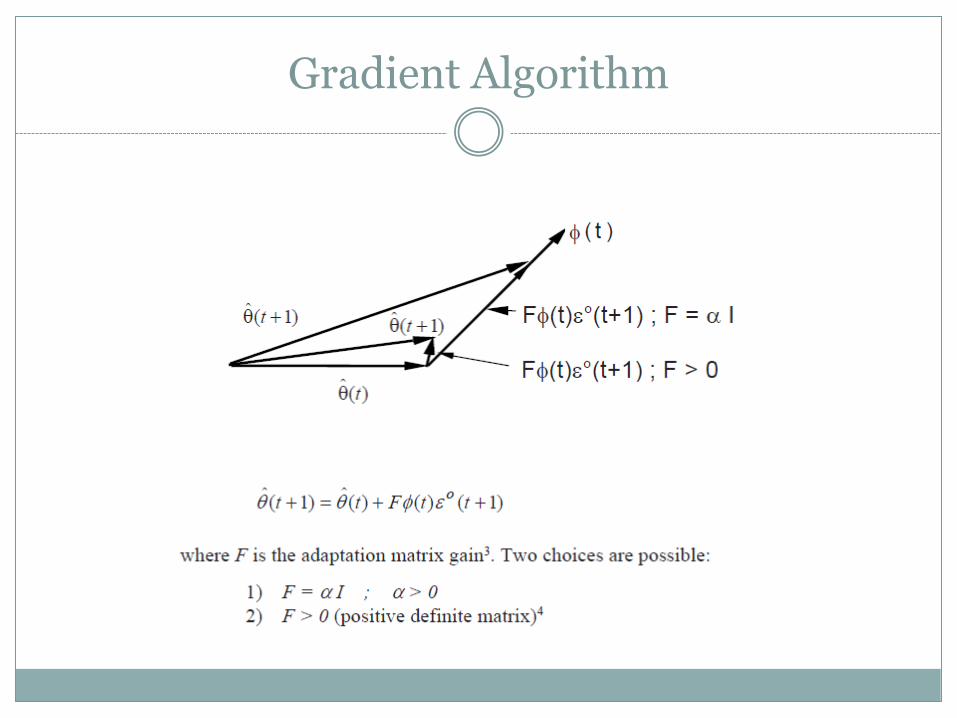
Gradient Algorithm

Objective is to minimize the error criterion

Gradient

Adaptation Gain

Gradient Algorithm

Gradient Algorithm

Therefore

Recall

And

Gradient Algorithm

Estimate Improvement

Compare to priori estimate

Better Estimate

Estimate Improvement

Error Criterion:

Update Equation:

The error:

Update Equation becomes:

using

Gradient Algorithm

Least Squares Algorithm

Gradient Method:

Least Square Method

Least Square Algorithm

Then, we can calculate a non-recursive parameter estimation

where

Recursive Least Squares Algorithm

Adaptation Gain

Formula can be generalized as

Different Identification Models

Input Sequences: The Problem

Input Sequence: PRBS

Effects of Disturbances

The plant measured output is in general contaminated by noise. This is due either to the effect of random disturbances acting at different points of the plant, or to measurement noises.

These random disturbances are frequently modeled by ARMA

models The plant plus the disturbance are modeled by an ARMAX

model. These disturbances introduces errors in the identification

models. This type of error is called bias of parameters.


Consider the effect of the random disturbances on the least square algorithm

The equation for the least square equation for N samples becomes


To get unbiased equations, the following must be true

Therefore, unbiased estimation happens only if the measurements and the noise are uncorrelated

In order for this to happen, w(t) must be white noise


Consider ARMAX model

Therefore,

If modeling white noise, we get


The prediction error becomes

Recall that


To avoid bias

Recursive Identification Methods: Structure

Structures

Identification Methods Type I

Identification Methods Based on the Whitening of the Prediction Error

Recursive Least Squares (RLS)

Extended Least Squares (ELS)

Recursive Maximum Likelihood (RML)

Output Error with Extended Prediction Model (OEEPM)

Generalized Least Squares (GLS)

Validation of Type I Methods

1. Creation of an I/O file for the identified model (using the same input sequence as for the system)

2. Creation of a prediction error file for the identified model (minimum 100 samples)

3. Whiteness test on the prediction errors sequence (also known as residual prediction errors)

Whiteness Test

Identification Methods Type II

Identification Methods Based on the Uncorrelation of the Observation Vector and the Prediction Error

Instrumental Variable with Auxiliary Model (IVAM)

Output Error with Fixed Compensator (OEFC)

Output Error with Filtered Observations (OEFO)

Output Error with Adaptive Filtered Observations (OEAFO)

Validation of Type II Methods

1. Creation of an I/O file for the identified model (using the same input sequence as for the system)

2. Creation of files for the sequences: system output, model output, residual output prediction error). These files must contain at least 100 samples

3. Uncorrelation test between the residual output prediction error sequence and the delayed prediction model output sequences

Incorrelation Test

SI Software

Practical Aspects

I/O Data Acquisition

Signal Conditioning

Selecting Model Complexity

Examples: Identification of DC Motor

References

Digital Control Systems: Design, Identification, and Implementation (Chapter 5, 6, and 7)

Landau and Zito

mechatronics system design - philadelphia …. system... · dr. tarek a. tutunji advanced modeling...

Documents