mechanistic analytical modeling of superscalar in … · mechanistic analytical modeling of...

50

Mechanistic Analytical Modeling of Superscalar In-OrderProcessor Performance

MAXIMILIEN B. BREUGHE, STIJN EYERMAN, and LIEVEN EECKHOUT,Ghent University, Belgium

Superscalar in-order processors form an interesting alternative to out-of-order processors because of theirenergy efficiency and lower design complexity. However, despite the reduced design complexity, it is nontrivialto get performance estimates or insight in the application–microarchitecture interaction without runningslow, detailed cycle-level simulations, because performance highly depends on the order of instructions withinthe application’s dynamic instruction stream, as in-order processors stall on interinstruction dependencesand functional unit contention. To limit the number of detailed cycle-level simulations needed during designspace exploration, we propose a mechanistic analytical performance model that is built from understandingthe internal mechanisms of the processor.

The mechanistic performance model for superscalar in-order processors is shown to be accurate with anaverage performance prediction error of 3.2% compared to detailed cycle-accurate simulation using gem5. Wealso validate the model against hardware, using the ARM Cortex-A8 processor and show that it is accuratewithin 10% on average. We further demonstrate the usefulness of the model through three case studies:(1) design space exploration, identifying the optimum number of functional units for achieving a givenperformance target; (2) program–machine interactions, providing insight into microarchitecture bottlenecks;and (3) compiler–architecture interactions, visualizing the impact of compiler optimizations on performance.

Categories and Subject Descriptors: C.0 [Computer Systems Organization]: General—Modeling of com-puter architecture; C.4 [Computer Systems Organization]: Performance of Systems—Modeling techniques

General Terms: Design, Experimentation, Measurement, Performance

Additional Key Words and Phrases: Superscalar in-order processors, processor design space exploration,functional units, inter-instruction dependences, performance modeling, cycle stacks

This research is funded through the European Research Council under the European Community’s SeventhFramework Programme (FP7/2007-2013)/ERC grant agreement no. 259295, as well as EU FP7 Adept projectnumber 610490.Authors’ addresses: M. B. Breughe, S. Eyerman, and L. Eeckhout, ELIS Department, Ghent University, Sint-Pietersnieuwstraat 41, B-9000 Gent, Belgium; email: [email protected], [email protected] article is an extension of “A Mechanistic Performance Model for In-Order Processors,” by Maximi-lien Breughe, Stijn Eyerman, and Lieven Eeckhout, presented at the 2012 International Symposium onPerformance Analysis of Systems and Software (ISPASS). The new contributions are:

—We added modeling of an arbitrary number of functional units of any type in contrast to a fixed number inthe ISPASS paper (i.e., 4 ALUs and 1 unit for all other types).

—We completely revised the modeling of interinstruction dependences and unified it with the functionalunit contention modeling.

—We added modeling of memory-level parallelism, which has a nonnegligible impact on performance forsome benchmarks that were not evaluated in the ISPASS paper.

—We validated the model against hardware.—We added a case study on sizing the number of functional units.—We reevaluated all other case studies using the new model and revealed new insights about the interaction

between dependences and functional unit contention.

Permission to make digital or hard copies of part or all of this work for personal or classroom use is grantedwithout fee provided that copies are not made or distributed for profit or commercial advantage and thatcopies show this notice on the first page or initial screen of a display along with the full citation. Copyrights forcomponents of this work owned by others than ACM must be honored. Abstracting with credit is permitted.To copy otherwise, to republish, to post on servers, to redistribute to lists, or to use any component of thiswork in other works requires prior specific permission and/or a fee. Permissions may be requested fromPublications Dept., ACM, Inc., 2 Penn Plaza, Suite 701, New York, NY 10121-0701 USA, fax +1 (212)869-0481, or [email protected]© 2014 ACM 1544-3566/2014/12-ART50 $15.00

DOI: http://dx.doi.org.10.1145/2678277

ACM Transactions on Architecture and Code Optimization, Vol. 11, No. 4, Article 50, Publication date: December 2014.

http://dx.doi.org.10.1145/2678277

50:2 M. B. Breughe et al.

ACM Reference Format:Maximilien B. Breughe, Stijn Eyerman, and Lieven Eeckhout. 2014. Mechanistic analytical modeling ofsuperscalar in-order processor performance. ACM Trans. Architec. Code Optim. 11, 4, Article 50 (December2014), 26 pages.DOI: http://dx.doi.org.10.1145/2678277

1. INTRODUCTION

For studying processor performance, both researchers and designers heavily rely ondetailed cycle-accurate simulation. Although detailed simulation provides accurateperformance projections for a particular design configuration, deriving fundamentalinsight into the interactions that take place within a processor is more complicated.Understanding trend behavior of microarchitecture structure scaling and the interac-tions among microarchitecture structures, as well as how the microarchitecture inter-acts with its workloads, requires a very large number of simulations. The slow speed ofdetailed cycle-accurate simulation makes it a poor fit to understand these fundamentalmicroarchitecture–application interactions.

In this article, we focus on mechanistic analytical performance modeling, which isa better method for gaining insight and for reducing the large number of detailedsimulations in large design spaces. Mechanistic modeling is derived from the actualmechanisms in the processor. A mechanistic model has the advantage of directly dis-playing the performance effects of individual mechanisms, expressed in terms of pro-gram characteristics such as interinstruction dependence profiles and fine-grainedinstruction mix; machine parameters such as processor width, number of functionalunits, and pipeline depth; and program–machine interaction characteristics such ascache miss rates and branch misprediction rates. Mechanistic modeling is in contrastto the more common empirical models that use machine learning techniques and/orstatistical methods (e.g., neural networks, regression) to infer a performance model[Dubach et al. 2007; Ipek et al. 2006; Joseph et al. 2006a, 2006b; Lee and Brooks 2006;Ould-Ahmed-Vall et al. 2007; Mariani et al. 2013]. Empirical modeling involves run-ning a large number of detailed cycle-accurate simulations to infer or fit a performancemodel. In contrast, mechanistic modeling builds a model from the internal structure ofthe processor and does not require simulation to infer or fit the model.

Detailed simulations or well-trained empirical models can show the performance im-pacts of different processor designs, but it is time-consuming and challenging at timesto reveal the underlying reason why a design improves performance for one applicationbut not another. Figure 1 illustrates this. Figure 1(a) shows that gsm_c and susan_shave a similar fraction of multiply instructions, yet Figure 1(b) shows that they behavedifferently when we increase the number of multipliers on the baseline microarchitec-ture from one to two (see Section 6 for a detailed description of the experimental setup).Mechanistic performance modeling provides a level of insight that enables quick anddeep understanding of such performance phenomena by breaking up total executiontime into different components that account for instruction latencies, dependences,cache misses, branch mispredictions, and so forth. (We refer back to this case study inSection 9.1.)

Whereas prior work in mechanistic performance modeling has focused on superscalarout-of-order processors [Eyerman et al. 2009; Karkhanis and Smith 2004], in this ar-ticle we propose a mechanistic model for superscalar in-order processors. Comparedto out-of-order processors, the performance of superscalar in-order processors is quitesensitive to the order of instructions in the dynamic instruction stream, interinstruc-tion dependences, instruction execution latencies, and the number of functional unitsavailable. Therefore, it is impossible to mimic the behavior of an in-order processorwith the existing models by constraining out-of-order resources (e.g., limiting the ROBsize to the pipeline width).


http://dx.doi.org.10.1145/2678277

Mechanistic Analytical Modeling of Superscalar In-Order Processor Performance 50:3

Fig. 1. Based on the instruction mix for gsm_c and susan_s (left graph), one would expect performance toimprove by adding an additional multiply unit. However, simulation results (right graph) show a significantperformance increase for gsm_c but not for susan_s.

We believe that this work is timely given that energy and power efficiency are pri-mary design concerns in contemporary computer system design. Whereas the focusis on extending battery lifetime in embedded systems, improving energy and powerefficiency also has important implications on cooling and total cost of ownership ofserver and data center infrastructures. In-order processors are less complex, consumeless power, and incur less chip area compared to out-of-order processors, which makesthem an attractive design point for specific application domains. In particular, in-orderprocessors are commonly used in the mobile space, ranging from cell phones to tabletsand netbooks; example processors are the Intel Atom (except for the recent Silvermontarchitecture) and ARM Cortex-A7/A8. For server throughput computing, integratingmany in-order processor cores on a single chip maximizes total chip throughput withina given power budget. Commercial examples include Sun Niagara [Kongetira et al.2005] and AMD/SeaMicro’s Intel Atom based server1; recent research projects havealso studied in-order processors for Internet-sector workloads [Andersen et al. 2009;Lim et al. 2008; Reddi et al. 2010].

The overall structure of the article is as follows. We start with a general overviewof the framework and a description of the assumed superscalar processor in Section 2.Next, we construct the mechanistic model in Sections 3 through 5. Our experimentalsetup is explained in Section 6. The evaluation in Section 7 shows that our modelreaches an average absolute prediction error of 3.2% compared to detailed cycle-levelsimulation with gem5. Further, Section 8 shows that our model can be used to predictthe performance of the ARM Cortex-A8 with an average absolute prediction error of10%. In Section 9, we demonstrate the usefulness of the model through three casestudies. We first leverage the model to understand program–machine interactions andreveal insight into the example just described in Figure 1. Second, we use the model tominimize the number of functional units while achieving a performance target of 98%compared to using a total of 16 functional units in a four-wide superscalar in-order pro-cessor. Third, we evaluate how compiler optimizations affect in-order performance andderive some interesting conclusions. We end by discussing related work in Section 10,by providing ideas for future work in Section 11, and by concluding in Section 12.

2. MODELING CONTEXT

Before describing the proposed model in great detail, we first set the context withinwhich we build the model. We present a general overview of the modeling framework,as well as a description of the assumed superscalar in-order processor architecture.

1http://www.seamicro.com/.


http://www.seamicro.com/


Fig. 2. Overview of the mechanistic modeling framework.

2.1. General Overview

The framework of the mechanistic model is illustrated in Figure 2. It requires a profilingrun to capture a number of statistics that are specific to the program only and areindependent of the machine. These statistics relate to the program’s instruction mixand interinstruction dependences, and need to be collected only once for each programbinary.

The profiling run also needs to collect a number of mixed program-machinestatistics—that is, statistics that are a function of both the program binary as wellas the machine configuration. Example statistics are cache and TLB miss rates, as wellas branch misprediction rates. Although, in theory, collecting these statistics requiresseparate runs for each cache, TLB and branch predictor configuration of interest; inpractice, however, most of these statistics can be collected in a single run. In particular,single-pass cache simulation [Hill and Smith 1989; Mattson et al. 1970] allows for com-puting cache miss rates for a range of cache sizes and configurations in a single run.We also collect branch misprediction rates for multiple branch predictors in a singlerun. Once these statistics are collected, we can predict cache miss rates and branchmisprediction rates for any combination of cache hierarchy with any branch predictorand any processor core configuration.

These statistics, along with a number of machine parameters, serve as input to theanalytical model, which then estimates superscalar in-order processor performance.The machine parameters include pipeline depth, pipeline width, number of functionalunits and their types, functional unit latency (multiply, divide, etc.), cache access la-tencies, and memory access latencies, as well as the configurations and sizes of caches,TLBs, and branch predictors.

Because the analytical model basically involves computing a limited number of for-mulas, a performance prediction is obtained almost instantaneously. In other words,once the initial profiling is done, the analytical model allows for predicting performancefor a very large design space in the order of seconds or minutes at most.

2.2. Microarchitecture Description

We assume a superscalar in-order processor with five pipeline stages: fetch (IF), de-code (ID), execute (EX), memory (MEM), and write-back (WB). IF and ID are referredto as the front-end stages of the pipeline, whereas EX, MEM, and WB are back-endstages. We consider a five-stage pipeline without loss of generality; we can model deeperpipelines by considering longer front-end pipelines and non–unit-latency instructionexecution units, as will become clear later. Each stage has W slots (numbered from 0to W − 1) to hold a total of W instructions, with W being the width of the processor. Weassume forwarding logic such that dependent instructions can execute back-to-backin subsequent cycles. Further, we assume stall-on-use—in other words, the proces-sor stalls on an instruction that consumes a value that has not been produced yet.



These instructions block in the ID stage. Load instructions perform address calcu-lation in the EX stage and perform the cache access in the MEM stage. Finally, weassume in-order commit to enable precise interrupts. This implies that instructionsthat take more than one cycle to execute (e.g., a multiply instruction or a cache miss)block all subsequent instructions from going to the WB stage. Since each stage canonly hold W instructions, this further implies that when a long-latency instructionblocks instructions from passing from the MEM stage to the WB stage, the EX stagewill eventually be filled with instructions, and hence no instructions can leave theID stage.

3. OVERALL FORMULA

The overall formula for estimating the total number of execution cycles T of an appli-cation on a superscalar in-order processor is as follows:

T = NW

+ Pmisses + Pdeps + PFU . (1)

In this equation, N equals the number of dynamically executed instructions, W standsfor the width of the processor, Pmisses is the total penalty due to miss events, Pdeps is thetotal penalty due to interinstruction dependences, and PFU stands for the penalty dueto functional unit limitations (i.e., structural hazards).

The intuition behind the mechanistic model is that the minimum execution timefor an application equals the number of dynamically executed instructions dividedby processor width—that is, it takes at least N/W cycles to execute N instructionson a W-wide processor in the absence of miss events and stalls. Miss events, inter-instruction dependences, and functional unit contention prevent the processor fromexecuting instructions at a rate of W instructions per cycle, which is accounted for bythe model by adding penalty cycles.

The next sections discuss each of the terms of the formula. We start with miss eventpenalties and then discuss instruction dependences and functional unit contention.

4. MISS EVENTS

We determine the penalty due to miss events using the following formula:

Pmisses =∑

i∈{missEvents}missesi × penaltyi. (2)

This formula computes the sum over the miss events, weighted with their respectivepenalties. We make a distinction between cache (and TLB) misses and branch mispre-dictions when it comes to computing the penalties.

4.1. Cache and TLB Misses

When an instruction cache miss occurs, the instructions in the front-end pipeline canstill enter the EX stage, but when the instruction cache miss is resolved, it takes sometime for the new instructions to refill the front-end pipeline. It is easy to understandthat the front-end pipeline drain time and refill time offset each other—that is, thepenalty for an instruction cache miss is independent of the front-end pipeline depth.In case of a data cache miss, the MEM stage blocks, and no instructions can leave orenter the EX stage until the data cache miss is resolved.

From the preceding discussion, it follows that the penalty for both an instruction anddata cache miss equals its miss latency (i.e., the access time to the next level of cacheor main memory). However, some instructions can complete execution in parallel withthe miss penalty. In case of an instruction cache miss on a four-wide processor, one,



two, or three instructions could have already been fetched before the instruction cachemiss occurred. Similarly, for a data cache miss, depending on the slot number at whichthe load instruction enters the MEM stage, one (the load instruction enters the MEMstage at slot 1), two (the load instruction enters at slot 2), or three older instructions(the load instruction enters at slot 3) can proceed to the WB stage. These instructionscan complete underneath the cache miss and are therefore hidden. Assuming thatcache misses are uniformly distributed across a W-wide instruction group, the averagenumber of instructions hidden underneath a cache miss equals W−1

2 . This means thatthe miss penalty can be reduced by W−1

2W cycles (which is less than one cycle). The totalpenalty for a cache or TLB miss thus equals

penaltycacheMiss = MissLatency − W − 12W

. (3)

Memory-level parallelism. Memory-level parallelism (MLP) is defined as the num-ber of simultaneously outstanding misses if at least one is outstanding [Chou et al.2004]. This implies that we only have to account for the first, nonoverlapped memoryaccess latency, as independent memory accesses later in the instruction stream arehidden underneath the first one. Out-of-order processors make use of this property byimplementing a reorder buffer and miss status handling registers (MSHRs) to exploitMLP over a large window of instructions. For in-order processors, on the other hand,this window is limited to the width W of the processor, and hence the amount of MLPis very low—that is, MLP can be exploited up until the instruction in the instructionstream that depends on the load miss (stall-on-use). When taking MLP into account,the penalty associated with the cache miss term in Formula (2) gets scaled as in thefollowing Formula (4):

PcacheMisses = cacheMissesi

MLP× penaltycacheMiss. (4)

As described by Van Craeynest et al. [2012], we can calculate the MLP as the numberof memory accesses between a load instruction and its first consumer, since this con-sumer blocks the ID stage. However, since the processor can only hold W instructionsper pipeline stage, the load instruction will block any instruction at a distance largerthan (W −1) instructions from proceeding to the next stage. This implies that we neverneed to account for memory accesses outside of a window larger than W instructions,even if the first consumer of the load is further than (W − 1) instructions apart. Wehave implemented a simple profiler that determines the average dependence distancebetween a load and its first consumer with the interinstruction dependence profile.We combine this with the fine-grained instruction mix profile to count the number ofindependent load instructions within this distance.

4.2. Branch Mispredictions

Branch mispredictions are slightly different from cache misses from a modeling per-spective. Upon a branch misprediction, all instructions fetched after the mispredictedbranch need to be flushed. In particular, when a branch misprediction is detected in theEX stage, all instructions in the front-end pipeline, as well as the instructions fetchedafter the branch in the EX stage, need to be flushed. Hence, the penalty of a branchmisprediction equals

penaltybranchMiss = D + W − 12W

, (5)

with D the depth of the front-end pipeline. The first term is the number of cycleslost due to flushing the front-end pipeline: there are as many cycles lost as there are



Fig. 3. Pattern distribution matrix generation for part of the dct_chroma routine of the h264 benchmark.

front-end pipeline stages, namely D. The second term is the penalty of flushing instruc-tions in the EX stage; this number ranges between 0 and W − 1. We again assume auniform distribution.

Correctly predicted branches may also introduce a performance penalty. In our setup,a branch is predicted one cycle after it was fetched, and if it is predicted taken, theinstruction(s) in the IF stage and the instructions in the ID stage that are youngerthan the branch (which were fetched assuming a nontaken branch) need to be flushed,incurring a pipeline bubble. This incurs 1 + W−1

2W penalty cycles per branch that ispredicted taken, even if it is correctly predicted. We will refer to this penalty as thetaken-branch hit penalty.

5. INTERINSTRUCTION DEPENDENCES AND FUNCTIONAL UNIT CONTENTION

To determine the penalty caused by interinstruction dependences and functional unitcontention, we need to keep track of (1) the distance between dependent instructions(the smaller the distance, the more likely the processor will stall to resolve the depen-dence) and (2) the order in which different instructions execute (subsequent instruc-tions of the same type will put more pressure on the specific functional unit). In manycases, instructions will suffer from both dependences on prior instructions and fromcontention on functional units. We therefore summarize this information collectivelyin the pattern history distribution matrix (H-matrix), which we will use to calculatethe penalty caused by interinstruction dependences and functional unit contention.Before explaining the formula, we will first illustrate how the H-matrix is constructed.Each instruction in the dynamic instruction stream can be represented by recordingthe history of the types of the W − 1 previous instructions, which we call a pattern,together with the distance to the closest instruction on which it depends. We can usethis pattern i and dependence distance j as row and column indices, respectively, toincrement a counter in the H-matrix for each instruction. As a result, the elementsof the H-matrix represent counters that indicate the occurrences of pattern i with adependence distance of j.

Figure 3 illustrates this using a small portion of the dynamic instruction flow ofthe dct_chroma routine of h264 on the left, together with its associated H-matrix onthe right. For the ease of visualization, each assembly instruction is represented by a



symbol that indicates the type of instruction: A stands for an ALU instruction, M for amultiply/divide, L for a load, and X for all other instructions that are not needed for thepenalty calculation (e.g., store instructions).2 To construct the H-matrix, we make useof a sliding window that slides through the whole instruction stream, instruction byinstruction. The size of the window equals the maximum processor width W of interest,which we set to 4 here and in all subsequent examples (unless stated otherwise). Foreach last instruction in the window, we record the distance to the closest instructionon which it depends together with the history of preceding instructions in the orderexecuted from old (left) to most recent (right). Consider the position of the slidingwindow in Figure 3. The last instruction in the window is an ALU instruction, andthe history pattern of instructions is denoted by MAAA. The last instruction has adependence on the multiply instruction at distance 3 (as indicated by the red arrow).Therefore, we increment the H-matrix counter at the row with pattern MAAA andthe column that represents dependence distance 3. We can now shift the window oneinstruction down to increment a counter for pattern AAAA at distance 1. We continuethis process for all instructions.

By associating a penalty term to each row and column in the H-matrix, we candetermine a cost matrix C. The C-matrix represents the cost (in number of cycles) thata specific history/dependence pattern incurs on the performance of the processor. Bymultiplying the matrices C and H term-wise and by accumulating them (i.e., takingthe Frobenius product), we can calculate the total penalty term for functional unitcontention and interinstruction dependences, as shown in Formula (6):

Pdeps + PFU =∑

i∈patterns,d=1..2×W

Ci,d × Hi,d = C : H. (6)

To determine the individual terms in the C-matrix (i.e., the cost associated witha specific history pattern and dependence distance), we need to determine (1) thepenalty for the specific history pattern assuming that there are no dependences and(2) the penalty for the specific dependence distance assuming a sufficient number offunctional units. In case an instruction waits both for a dependence to resolve and for afunctional unit to become available, the largest of those two penalties will be accountedfor, as shown in Formula (7):

Ci,d = max(cdep(i, d), c f u(i)

). (7)

cdep(i, d) represents the penalty of pattern i when the last instruction in the patternhas a dependence distance d. c f u(i) is the penalty caused by functional unit contentionfor pattern i—in other words, when multiple instructions from the same instructiontype reside in pattern i, we need to account a penalty waiting for an appropriate unitto start processing the last instruction of pattern i. The terms cdep(i, d) and c f u(i) arethe subject of the following subsections.

Although Formula (6) shows how the sum of dependence penalties and functionalunit contention penalties can be calculated together, we will show in Section 9.1 howwe can determine these penalties separately.

5.1. Interinstruction Dependences

5.1.1. Dependences on Unit-Latency Instructions. In this section, we derive the penaltyof an instruction that depends on the outcome of a close-by (within W instructions)

2X stands for don’t care instructions, as these instructions do not contribute to the penalty calculation fordependences and functional unit contention. Note that in the remainder of the article, we will mark otherinstructions irrelevant for the calculation with X.



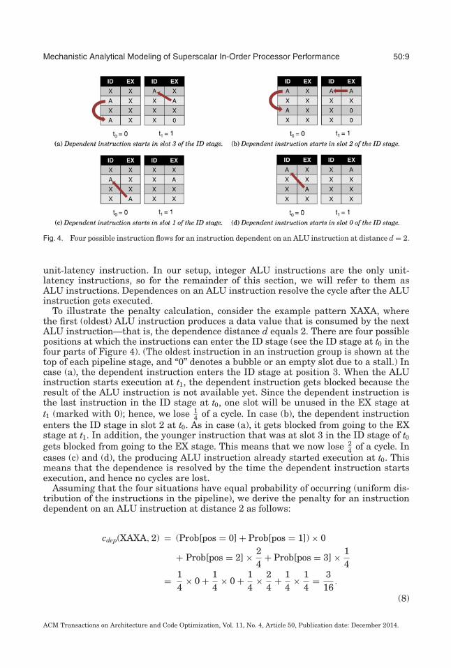
Fig. 4. Four possible instruction flows for an instruction dependent on an ALU instruction at distance d = 2.

unit-latency instruction. In our setup, integer ALU instructions are the only unit-latency instructions, so for the remainder of this section, we will refer to them asALU instructions. Dependences on an ALU instruction resolve the cycle after the ALUinstruction gets executed.

To illustrate the penalty calculation, consider the example pattern XAXA, wherethe first (oldest) ALU instruction produces a data value that is consumed by the nextALU instruction—that is, the dependence distance d equals 2. There are four possiblepositions at which the instructions can enter the ID stage (see the ID stage at t0 in thefour parts of Figure 4). (The oldest instruction in an instruction group is shown at thetop of each pipeline stage, and “0” denotes a bubble or an empty slot due to a stall.) Incase (a), the dependent instruction enters the ID stage at position 3. When the ALUinstruction starts execution at t1, the dependent instruction gets blocked because theresult of the ALU instruction is not available yet. Since the dependent instruction isthe last instruction in the ID stage at t0, one slot will be unused in the EX stage att1 (marked with 0); hence, we lose 1

4 of a cycle. In case (b), the dependent instructionenters the ID stage in slot 2 at t0. As in case (a), it gets blocked from going to the EXstage at t1. In addition, the younger instruction that was at slot 3 in the ID stage of t0gets blocked from going to the EX stage. This means that we now lose 2

4 of a cycle. Incases (c) and (d), the producing ALU instruction already started execution at t0. Thismeans that the dependence is resolved by the time the dependent instruction startsexecution, and hence no cycles are lost.

Assuming that the four situations have equal probability of occurring (uniform dis-tribution of the instructions in the pipeline), we derive the penalty for an instructiondependent on an ALU instruction at distance 2 as follows:

cdep(XAXA, 2) = (Prob[pos = 0] + Prob[pos = 1]) × 0

+ Prob[pos = 2] × 24

+ Prob[pos = 3] × 14

= 14

× 0 + 14

× 0 + 14

× 24

+ 14

× 14

= 316

.

(8)



In general, we can calculate the penalty for an instruction dependent on an ALUinstruction at distance d (with d < W) using the following formula:

cdep(i, d < W) =W−1∑j=0

Prob [pos = j|pat = i] ×{

W− jW if d ≤ j

0 else(9)

=W−1∑j=d

1W

× W − jW

(10)

= (W − d) (W − d + 1)2W2 . (11)

In this equation, i represents the pattern, W the processor width, d the dependencedistance to the closest ALU instruction, and Prob [pos = j|pat = i] the probability thatthe newest instruction in the pattern i is at position j in the ID stage. Note that ican be any pattern, with the constraint that the (d + 1)-th symbol is an “A”-symbol(i.e., the producer is an ALU instruction). The inequality j ≥ d indicates that we onlyneed to account penalty when the producing ALU instruction is in the ID stage atthe same cycle. In Formula (10), we make use of the assumption that instructions areuniformly distributed in the pipeline stage. We find this assumption to be accuratefor the set of benchmarks used in our setup. However, one could conceive a cornercase application that is dominated by instructions with dependence distances of 1that causes all instructions to be serialized. Hence, most of the instructions of thisapplication will enter the first slot of the ID stage. To model these corner cases, one couldestimate the probabilities with a heuristic based on the overall average dependencedistance: if the average dependence distance is close to 1, more weight needs to begiven to Prob[pos = 0]. However, we found this case to be very rare in our setup, andmodeling it increases the complexity of the model without noticeably improving itsaccuracy.

5.1.2. Dependences on Load Instructions. Unlike ALU instructions, load instructions donot produce their result in the EX stage but in the MEM stage. This has two conse-quences for calculating the penalty caused by instructions dependent on a load instruc-tion. First, this means that if a load instruction and its consumer reside in the ID stagein the same cycle, an additional penalty cycle will need to be accounted for on top ofthe one calculated with Formula (11). Second, even when the load instruction and itsdependent instruction reside in consecutive stages (load in the EX stage, dependentinstruction in the ID stage), a penalty needs to be accounted for.

When 0 < d < W, the load instruction can either be in the same stage or in a consec-utive stage as the dependent instruction. When W ≤ d < 2W , the load instruction andthe dependent instruction can never reside in the same stage, and hence we will onlyneed to account a penalty when they reside in consecutive stages.

The reasoning for calculating the penalty when W ≤ d < 2W is fairly similar as fordependences on ALU instructions where d < W . We can find the penalty for depen-dences on load instructions for a dependence distance W ≤ d < 2W by substituting dby d − W in Formula (10):

cdep(i, d ≥ W) =W−1∑

j=d−W

1W

× W − jW

(12)

= (2W − d + 1)(2W − d)2W2 . (13)



For 0 < d < W , the penalty can be calculated using Formulas (14) and (15). The firstterm in Formula (14) reflects that for d < W , we always need to account a penalty, sinceboth instructions either reside in the same stage or in consecutive stages. The secondterm reflects that if both the dependent instruction and the load instruction reside inthe ID stage at the same time, we need to account an additional cycle:

cdep(i, d < W) =W−1∑j=0

1W

× W − jW

+W−1∑j=d

1W

× 1 (14)

= 3W + 1 − 2d2W

. (15)

5.1.3. Dependences on Long-Latency Instructions. Other long-latency instructions, such asinteger multiply instructions, wait in the MEM stage until their result is calculated.Therefore, instructions that depend on long-latency instructions are penalized thesame way as instructions that depend on load instructions (see Formulas (15) and (13)for 0 < d < W and W ≤ d < 2W , respectively). Note that the latency of the long-latency instruction itself will be accounted for as a functional unit penalty (see thenext section), so for the dependent instruction, we only have to account for the emptyissue slots between the long-latency instruction and the dependent instruction.

However, as we will show in Sections 5.2.2 and 5.2.3, long-latency instructions cansometimes be executed in parallel, depending on the number of functional units avail-able. As a result, no penalty is accounted to the instruction executing in parallel withanother instruction. However, if there is a dependence between these instructions, thelatency will not be hidden. We account for this by adding the latency of the long-latencyinstruction to the dependence penalty if the closest dependent instruction is of the sametype.

5.2. Functional Unit Contention

5.2.1. ALU Contention. We first derive the penalty for integer ALU instructions dueto functional unit contention. We model ALU contention penalties in a way that isanalogous to dependence penalties on ALU instructions. For this, we need to define ananalogy to the dependence distance:

dU (i) : distance to the instruction that causes functional unit contentionwhen the processor has U units, for pattern i.

For example, for a superscalar processor of width W = 4 with two ALUs, the contentiondistance for pattern XAAA, dU (XAAA), equals 2, because the last instruction in thegroup can only start execution when the first one (at distance 2) finished its execution.

Replacing the dependence distance d with dU (i) in Formula (10) allows us to deter-mine the ALU contention penalty:

c f u(i) = fr(i) =W−1∑j=0

Prob [pos = j|pat = i] ×{

W− jW if dU (i) ≤ j

0 else

=W−1∑

j=dU (i)

Prob [pos = j|pat = i] × W − jW

(16)

≈ (W − dU (i))(W − dU (i) + 1)2W2 . (17)



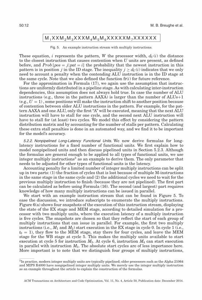
Fig. 5. An example instruction stream with multiply instructions.

These equation, i represents the pattern, W the processor width, dU (i) the distanceto the closest instruction that causes contention when U units are present, as definedbefore, and Prob [pos = j|pat = i] the probability that the newest instruction in thispattern is in position j in the ID stage. The inequality j ≥ dU (i) indicates that we onlyneed to account a penalty when the contending ALU instruction is in the ID stage atthe same cycle. Note that we also defined the function fr(i) for future reference.

For the approximation in Formula (17), we again use the assumption that instruc-tions are uniformly distributed in a pipeline stage. As with calculating inter-instructiondependencies, this assumption does not always hold true. In case the number of ALUinstructions (e.g., three in the pattern AAXA) is larger than the number of ALUs+1(e.g., U = 1) , some positions will make the instruction shift to another position becauseof contention between older ALU instructions in the pattern. For example, for the pat-tern AAXA and one ALU, only the first “A” will be executed, meaning that the next ALUinstruction will have to stall for one cycle, and the second next ALU instruction willhave to stall for (at least) two cycles. We model this effect by considering the patterndistribution matrix and by accounting for the number of stalls per pattern. Calculatingthese extra stall penalties is done in an automated way, and we find it to be importantfor the model’s accuracy.

5.2.2. Nonpipelined Long-Latency Functional Units. We now derive formulas for long-latency instructions for a fixed number of functional units. We first explain how tomodel nonpipelined units and then discuss pipelined units in Section 5.2.3. Althoughthe formulas are general enough to be applied to all types of functional units, we useinteger multiply instructions3 as an example to derive them. The only parameter thatneeds to be adjusted for other types of functional units is the latency.

Accounting penalty for a limited number of integer multiply instructions can be splitup in two parts: (1) the fraction of cycles that is lost because of multiple M-instructionsin the same stage in the same cycle and (2) the additional cycles we need to wait for theprevious multiply instruction to finish (because they are not pipelined). The first partcan be calculated as before using Formula (16). The second (and largest) part requiresknowledge of how many multiply instructions can be issued in parallel.

We start with an example instruction stream that can be found in Figure 5. Toease the discussion, we introduce subscripts to enumerate the multiply instructions.Figure 6(a) shows four snapshots of the execution of this instruction stream, displayingthe state of the EX stage and MEM stage, according to detailed simulation for a pro-cessor with two multiply units, where the execution latency of a multiply instructionis five cycles. The snapshots are chosen so that they reflect the start of each group ofmultiply instructions that can issue in parallel. For example, the first two multiplyinstructions (i.e., M1 and M2) start execution in the EX stage in cycle 0. In cycle 1 (i.e.,t0 = 1), they flow to the MEM stage, stay there for four cycles, and leave the MEMstage for the WB stage at cycle 5. This makes the multiply units available to startexecution at cycle 5 for instruction M3. At cycle 6, instruction M4 can start executionin parallel with instruction M3. The absolute start cycles are of less importance here.More important is to note that we distinguish four groups of multiply instructions,

3In practice, modern integer multiply units are typically pipelined; older processors such as the Alpha 21064and MIPS R4000 have nonpipelined integer multiply units. We merely use the integer multiply instructionas an example throughout the article to explain the construction of the formulas.



Fig. 6. Instruction flow of the example instruction stream in Figure 5 through a superscalar processor withtwo multiply units.

Table I. Pattern Distribution for the Instruction Stream inFigure 5 and Penalties Assuming Two Multiply Units

Nonpipelined PipelinedPattern Frequency Penalty PenaltyXXXM 3 latency − 1 latency − 1MXXM 1 0 0XXMM 2 0 0XMMM 1 latency − 1 0

meaning that we penalize the performance by four times the multiply latency for theseven “M”-instructions.

The challenge now is to calculate the penalty while having limited information com-pared to detailed simulation—that is, using only the pattern distributions of the H-matrix (Table I). With Formula (16), we can calculate the fraction of cycles lost becausethere are more multiply instructions than multiply units available at the same time inthe same stage. To determine the parallelism of multiply instructions that can get exe-cuted at the same time, we can again use the pattern distribution matrix. We considerpatterns that end with an M-symbol and account an appropriate penalty, based on thetotal number of M-symbols in the pattern.

For the example where we have two multiply units, we do not need to account penaltyfor patterns with exactly two M-symbols, as the right-most multiply instruction can beissued in parallel with the previous one. This is also true when all four instructions inthe pattern are multiply instructions. If, however, the right-most instruction is the onlymultiply instruction or if it is the third multiply instruction, the full penalty needs tobe accounted for. For the example instruction stream of Figure 6, the distribution andpenalties of patterns ending in with an M-symbol can be found in the second and thirdcolumns of Table I.

In general, we can derive the following formula to calculate the total cost for executinga long-latency instruction for an arbitrary number of units:

c f u(i) = fr(i) +{

latency − 1 if (#insns(i) mod U ) = 10 else.

(18)



In Formula (18), U is the number of units of this type of long-latency instruction, and#insns(i) represents the number of instructions of this type in pattern i. The intuitionbehind this formula is that the first multiply instruction will appear as an XXXMpattern, for which we account the full penalty. The second multiply instruction will seethe first instruction as an older instruction in its pattern (e.g., XMXM), so we do notneed to account a penalty if there are two or more multiply units.

However, Formula (18) can lead to underestimations in situations where we havea dense concentration of multiply instructions (e.g., XXXMMMMMMMM would beaccounted only two times the latency instead of four, because all of the MMMM patternshave no latency). This can be solved by modifying the previous formula as follows:

c f u(i) = fr(i) +{

latency − 1 if(#insts(i) mod U

) = 1latency−1

min(U,#insts(i)) × Pr[dense|pattern = i] else.(19)

Here, Pr[dense|pattern = i] is the probability that pattern i appears in a dense concen-tration of multiply instructions. We estimate this probability by counting the frequencyof occurrence from the pattern distribution matrix.

5.2.3. Pipelined Long-Latency Functional Units. We now move to modeling the impact oflong-latency instructions that execute on pipelined functional units. Pipelined func-tional units have the advantage that they are capable of executing a new instructionevery cycle, and hence they yield a potential performance improvement over non-pipelined execution, but they also require a more complex design. Because of in-orderexecution, however, there is a limit on the potential performance improvement: whena long-latency instruction is being executed, it will block all younger instructions frompassing the MEM stage (because of in-order commit). This will make the EX stage fillup with instructions, blocking younger instructions from starting execution. So, onlyinstructions that can make it into the EX stage can potentially execute in parallel.

In Figure 6(b), we illustrate what happens with the example of Figure 5 if themultiply units are pipelined. We distinguish three groups of multiply instructions thatcan be executed in parallel (assuming no dependences between them).

As before, we use the distribution matrix in Table I. To calculate the penalties, weagain account for two parts: the part in which we lose a fraction of a cycle because thereare more multiply instructions at the same time in the EX stage than multiply unitsavailable, and the part where we need to account for the latency of the multiplicationitself. For pipelined units, we only need to account for this latency if the current multiplyinstruction is the only multiply in the pattern. The fourth column in Table I shows thepenalties for pipelined units. Using these penalties and the distribution matrix, wecan account for the total penalty caused by long-latency instructions in the exampleinstruction stream.

In general, the penalty for long-latency instructions on pipelined functional unitscan be calculated with Formula (20). We only account a penalty if there is exactly onemultiply instruction in the pattern, because all other instructions can be executed inparallel. As is the case with nonpipelined functional units, we also account for a penaltyin case there is a high density of multiply instructions:

c f u(i) = fr(i,U ) +{

latency − 1 if #insts(i) = 1latency−1#insts(i) × P[dense|pattern = i] else.

(20)

6. EXPERIMENTAL SETUP

We use 19 benchmarks from the MiBench benchmark suite [Guthaus et al. 2001],which is a popular suite of embedded benchmarks from different application domains,including automotive/industrial, consumer, office, network, security, and telecom. Next



Table II. Parameter Settings for the Functional Units

Parameter Default Range Cortex-A8Integer ALUs (IA) 2 1 to 4 2Integer Multiply/ 1 1 to 4 1Divide Units (IM) nonpipelined nonpipelined/pipelined pipelinedFloating-Point ALUs (FA) 1 1 to 4 1

nonpipelined nonpipelined/pipelined nonpipelinedFloating-Point Multiply/ 1 1 to 4 merged withDivide Units (FM) nonpipelined nonpipelined/pipelined FA-unit

Table III. Default Parameter Settings

Parameter Default Cortex-A8Processor width 4 2Processor frequency 1GHz 1GHzPipeline depth 5 stages 13 stagesFP ALU latency 3 cycles 10 cyclesFP Multiply latency 15 cycles 17 cyclesFP Divide latency 15 cycles 65 cyclesFP MAC latency 15 cycles 26 cyclesFP Sqrt latency 15 cycles 60 cyclesInteger Multiply latency 5 cycles 3 cyclesInteger Divide latency 20 cycles NAL1 D- and I caches 128KB 32KB

4-way set assoc 4-way set assocL2 cache 4MB 256KB

8-way set assoc 8-way set assoc

to these MiBench benchmarks, we also use 15 benchmarks from SPEC CPU2006.We selected inputs from the KDataSets input database [Chen et al. 2010] so thateach MiBench benchmark executes approximately 1 billion instructions. For SPECCPU2006, we generated representative simulation regions of 1 billion instructionseach using SimPoint [Hamerly et al. 2005].

We use the gem5 simulation framework [Binkert et al. 2011]. We derive our profilerfrom gem5’s functional simulator, and we validate our model against detailed cycle-level simulation using gem5. Detailed simulation runs at 92 KIPS on an Intel XeonHarpertown (L5420) processor. Although our profiler is more than 10 times faster,running at 1.4 MIPS, profiles need be calculated only once for a whole range of processorconfigurations. With these profiles, we can quickly generate performance estimates byevaluating the preceding analytic formulas. This is done in a couple of seconds for thecomplete design space.

The parameters that we vary in the next sections are shown in Table II, along withthe default settings, which forms a design space of 2,048 configurations. For modelvalidation, we use a subset of 70 randomly selected configurations that span a broadrange of the design space of the total 2,048 configurations. Although our model canbe applied while varying many more parameters (such as pipeline width, depth, cachesizes, cache associativities, and branch predictor settings), in this article, our primaryfocus is on the processor core in which we vary the number and configuration of thefunctional units, as this is the most complicated part to model for superscalar in-orderprocessors. Table III shows the default settings for the other processor parameters. Werefer the interested reader to the earlier version of the model for results in which we



Fig. 7. Cumulative probability distribution of error for 70 configurations on SPEC CPU2006 and MiBench.

vary other processor parameters such as pipeline depth, width, cache configuration,and branch predictor (see Breughe et al. [2012]).

For hardware validation, we use a BeagleBone Black board with the Texas Instru-ments AM3358 Sitara ARM Cortex-A8 processor, running Debian GNU/Linux 7. Thecorresponding microarchitectural parameters can be found in the right-most columnsof Tables II and III and are based on the technical references from ARM Holdings[2010] and Texas Instruments Incorporated [2014]. Because the Cortex-A8 is an ARM-processor, we extended our profiler to capture profiles for the ARM ISA, in additionto the Alpha ISA, which is used for the validation against detailed simulation. Weused Linux’s built-in time command to measure user time, and we disable dynamicfrequency scaling by setting the processor to a fixed clock frequency of 1GHz in ourexperiments. To avoid generating new SimPoints for SPEC CPU2006 on ARM, andsetting up the framework to execute SimPoints on hardware, our hardware validationis limited to the MiBench suite.

7. VALIDATION AGAINST DETAILED SIMULATION

We validate the model against detailed simulation in two steps. First, we evaluateaccuracy by simulating a large range of different configurations. We consider 34 bench-marks and 70 configurations, and we compare the CPI values of detailed simulationversus the model. Figure 7 shows a cumulative plot comparing all simulated pointswith the model. From this figure, we can see that about 90% of all evaluated pointshave an error of less than 7% in CPI. Overall, the model has an error of 3.2% on average,with a maximum error of 13%.

Second, we evaluate how well the model tracks the relative difference on a numberof configurations: starting from the baseline configuration, we increase the numberof available functional units. We also study the effect of pipelining functional units.We start by studying the effect of adding floating-point multiply units to our baselineconfiguration. As can be seen in Figure 8, adding a second multiply unit decreasesCPI significantly. (This graph shows results for the floating-point benchmarks only;i.e., the other benchmarks do not see a performance impact from varying the numberof floating-point units.) Four multiply units reduces CPI only for a few benchmarks.These trends are tracked accurately by our model. On average, the model has an errorof only 2.1% for the configurations in this experiment and a maximum error of 5.5%.



Fig. 8. Model validation while varying the number of floating-point multiply units (FM) for the floating-pointbenchmarks of MiBench and SPEC CPU2006.

Fig. 9. Evaluation of the model compared to detailed simulation for pipelined (P) and nonpipelined (NP)functional units on SPEC CPU2006.

Fig. 10. Evaluation of the model compared to the Cortex-A8 microarchitecture.

We now look at the impact of pipelining all of the units (i.e., integer multiply/divideunit, floating-point ALU, and floating-point multiply/divide unit) of the baseline con-figuration, as shown in Figure 9. Due to space constraints, we only plot results forSPEC CPU2006; we obtain similar results for the MiBench benchmarks. We observean average absolute error of 2% and a maximum error of 7.6%.

8. HARDWARE VALIDATION

Figure 10 shows CPI values for our set of 19 MiBench benchmarks when executedon the Cortex-A8 processor, along with the prediction of our model. We find that theaverage absolute prediction error is 10%, with 12 benchmarks showing an error of lessthan 8%; the maximum error equals 32% for adpcm_d. Overall, the model is fairlyaccurate, taking into account that we did not make important changes to the model



compared to the ALPHA/gem5 model. The only changes are adjustments to the profilerto be compatible with the ARM ISA and modeling Cortex A8’s variable latencies forfloating-point instructions.

More specifically, to improve the accuracy of the floating-point benchmarks, we re-quired a more fine-grained breakdown of the floating-point instruction mix (i.e., mul-tiply, division, multiply-accumulate, and square root). We then use this fine-grainedinstruction mix together with instruction latencies found in the Cortex-A8 technicalreference [ARM Holdings 2010] to generate a weighted average of the overall floating-point latency and feed it into our model.

Several adjustments to the model could be made to improve accuracy even further.The gem5 models an fetch buffer with the size of an entire cache line, as observedby Gutierrez et al. [2014], which underestimates the number of instruction cache ac-cesses in gem5. Because our original modeling efforts are targeted at a microprocessorsimilar to gem5’s in-order core, we make the same assumptions on the fetch buffer.For example, gsm_c is an application within the top three benchmarks with most in-struction cache misses, indicating that its instruction footprint is non–cache resident,and hence modeling a smaller fetch buffer would correctly predict a higher executiontime. Furthermore, we are unaware of the branch prediction latency of the Cortex-A8,whereas we model taken branches with 1 cycle of penalty. In addition, Gutierrez et al.[2014] show that gem5’s branch prediction accuracy decreases for low MPKI values.Both of these branch predictor inaccuracies could explain our performance underesti-mation of adpcm_d. Further, the Cortex-A8 does not allow executing two instructionsin the same slot if they have output dependences (WAW dependences), whereas ourmodel abstracts this away. This likely impacts the overall performance overestimation.Finally, we assume a fixed memory latency, whereas DRAM latency tends to dependon the physical memory addresses for which requests are made. As correctly statedby Desikan et al. [2001], this depends on the virtual to physical page mappings of thenative system and is quite difficult to replicate. We find that benchmarks spending alot of time in system calls, such as tiff2rgba and tiffmedian, indeed show performanceoverestimations.

9. CASE STUDIES

9.1. Revealing Performance Bottlenecks

In our first case study, we use the model to understand the performance numbers ofthe example in the introduction of the article (see Figure 1(b)).

Formula (1) derives the number of execution cycles of an application on a targetmicroprocessor as a sum of terms. This property is useful in determining performancebottlenecks. By identifying the largest contributors to the execution cycles, one can findthe most promising directions to improve performance. For example, suppose that thepenalty due to data cache misses (part of the Pmisses term) is the largest contributor tothe execution cycles; performance could be improved by installing a larger cache or byimproving data locality. If, on the other hand, the penalty due to functional units (PFU )is relatively large, we can improve performance by adding functional units.

We now build CPI stacks for the benchmarks and configurations of Figure 1(b).Thereto, we divide the terms in Formula (1) by the total number of instructions N, andwe split up the terms Pmisses and PFU into smaller terms to get a better level of detail.The “base” component is the first term (i.e., N

W ), which becomes 1W when divided by N.

Pmisses can easily be split up by multiplying the number of miss events of each typewith their respective penalty as explained in Section 4.

Since PFU and Pdeps are modeled in a unified matrix C, we have to split up the matrixC into CFU and Cdeps to determine penalties for functional units and interinstruction



Fig. 11. CPI stacks reveal that interinstruction dependences between multiply instructions are the under-lying bottleneck that is preventing performance improvement for susan_s. The “other” component is all otherterms in the model that only have a small component.

dependences separately. We do this similarly to how the matrix was constructed inFormula (7):

Cdeps(i, d) ={

cdep(i, d) ifcdep(i, d) > c f u(i)0 else

CFU (i, d) ={

c f u(i, d) ifcdep(i, d) ≤ c f u(i)0 else.

The term PFU can be further broken down into PintALU , PintMultiply, PfpALU , andPfpMultiply by accounting for the CFU (i, d) terms only, in which i denotes a patternassociated with that functional unit (i.e., the last instruction in pattern i executes onfunctional unit type FU ).

The CPI stacks for the benchmarks and configurations of Figure 1(b) are shownin Figure 11. Although the model has a small error on the performance prediction,it reveals why there is hardly any performance improvement for susan_s. With asingle multiply unit, we observe that the penalties due to integer multiplies (PintMultiply)are relatively high. When we add a second multiply unit, we see that this term issignificantly reduced for gsm_c, which can be explained by the many patterns withmore than one multiply instruction. For susan_s, we see that the PintMultiply term isalso reduced; however, the term Pdeps is increased by the same amount that PintMultiplywas reduced. The decrease in PintMultiply can again be explained by patterns consistingof multiple multiply instructions that can execute in parallel. However, the increasein Pdeps means that these multiply instructions depend on each other, which inhibitsparallel execution.

9.2. Minimizing the Number of Functional Units for a Given Performance Target

In our second case study, we use the model to minimize the number of units neededfor a specific performance target. We use gem5 to find the performance (expressed asIPC) of our baseline configuration (containing 5 functional units) and the maximumachievable performance when having 4 functional units of each type (i.e., a total of16 units). The harmonic mean of speedups over the baseline IPC equals 1.087. Themaximum speedup is observed for lame (1.52) and zeusmp (1.49).

We now use the model to find optimal configurations per benchmark (i.e., configu-rations with a minimum number of functional units), where we set the performancetarget at 98% of the maximum IPC. Detailed simulation of these optimized configu-rations confirms that these configurations indeed have an IPC of at least 98% of themaximum achievable IPC as predicted by the model, by using a minimum amount offunctional units. Figure 12 shows IPC numbers, resulting from detailed simulation, for



Fig. 12. Baseline performance, the performance of the configuration with four units of each type (Maximumunits), and the performance of the configuration picked by the model with a minimum number of functionalunits within 98% of the optimum (Optimized). The table aligned with the figure details the configurationpicked by the model: number of integer ALUs (IA), integer multiply/divide units (IM), floating-point ALUs(FA), and floating-point multiply/divide units (FM).

Fig. 13. Normalized cycle stacks for five benchmarks across different compiler optimizations.

a selection of benchmarks, along with the optimal number of units of each type. Becauseof space constraints, we only show the 20 benchmarks that have the largest delta inIPC between the baseline configuration and the configuration with a total of 16 func-tional units. (We obtain similar results for the other 14 benchmarks.) The “Optimized”bars represent the IPC results for the configurations found in the table that is alignedwith the figure. The bars “Baseline” and “Maximum units” represent our baseline of5 units, and the configuration with all 16 units, respectively. The harmonic mean of thespeedups of the optimized configurations over the baseline configuration equals 1.08(maximum speedup of 1.51 for lame and 1.47 for zeusmp). We observe that for 29 outof the 34 benchmarks, we only need 7 or fewer functional units to achieve at least 98%of the IPC with 16 functional units. The resulting configurations are nontrivial andtime-consuming to find using detailed cycle-accurate simulation, which motivates theuse of our fast model to guide design choices.

9.3. Compiler Optimizations

In our last case study, we use the model to study how compiler optimizations affectsuperscalar in-order performance (Figure 13). We consider -O3, -O3 without instruc-tion scheduling (-O3 -fno-schedule-insns), and -O3 with loop unrolling turned on



Fig. 14. Normalized cycle stacks for susan_s with and without loop unrolling, and on two different archi-tectures (one and two multiply units).

(-O3 -funroll-loops) for the five benchmarks for which we observed the largest im-pact due to compiler optimizations. Figure 13 shows normalized cycle stacks—that is,a cycle stack is computed by multiplying a CPI stack with the number of dynami-cally executed instructions; the cycle stacks are then normalized to the execution timewith the -O3 optimization level. For most of the benchmarks, instruction schedulingincreases the distance between dependent instructions, resulting in a lower penaltydue to dependences. For some benchmarks (e.g., gsm_c), the base component increasesslightly through instruction scheduling, meaning that the number of executed instruc-tions increases. The reason for this is the addition of spill code. However, the cost of spillcode is compensated for by the substantial decrease in the impact of interinstructiondependences.

Most of the benchmarks (and all of the ones in Figure 13) benefit from loop unrolling.Three components get an important reduction through loop unrolling. First, the numberof dynamic instructions decreases because fewer branches and loop iteration counterincrements are needed after loop unrolling. Second, because there are fewer branches,the penalty due to taken branches also decreases. Third, for susan_s, we observe thebiggest contribution from the smaller penalty due to interinstruction dependences;clearly, loop unrolling enables the instruction scheduler to better schedule instructionsso that fewer interinstruction dependences have an impact on in-order performance.

As shown in Section 9.1, dependences prevent a performance improvement whenthe number of multipliers is increased from one to two for susan_s. In Figure 14,we show normalized cycle stacks for susan_s without loop unrolling (-O3) and withloop unrolling enabled (-unroll) on the baseline architecture (one multiply unit) andon the baseline architecture with an additional multiply unit (two multiply units).As mentioned earlier, for -O3 the penalty for multiply instructions transforms intoa penalty for interinstruction dependences when a second multiply unit is added.When we enable loop unrolling, however, many of these additional interinstructiondependences can be removed because the instruction scheduler is now able to placeindependent multiply instructions (that were originally spread across loop iterations)closer together and dependent ones further apart. As a result, we see a considerableperformance gain when the number of multiply units is doubled for the loop-unrolledversion of susan_s.

10. RELATED WORK

We now describe prior work in analytical modeling, statistical modeling, and programcharacterization that is most related to our work.



10.1. Analytical Modeling

Basically, there are three approaches to analytical modeling: mechanistic modeling,empirical modeling, and hybrid mechanistic/empirical modeling.

Mechanistic modeling derives a model from the mechanics of the processor, and priorwork focused on mechanistic modeling of out-of-order processor performance for themost part. Michaud et al. [1999] build a mechanistic model of the instruction windowand issue mechanism. Karkhanis and Smith [2004] extend this simple mechanisticmodel to build a complete performance model that assumes sustained steady-stateissue performance punctuated by miss events. Chen and Aamodt [2008] improve on thismodel through more accurate modeling of pending data cache hits, overlaps betweencomputation and memory accesses, and the impact of a limited number of MSHRs.Taha and Wills [2008] propose a mechanistic model that breaks up the execution intoso-called macro blocks, separated by miss events. Eyerman et al. [2009] propose theinterval model for superscalar out-of-order processors. Whereas all of this prior workfocused on out-of-order processors, Breughe et al. [2011] proposed a mechanistic modelfor scalar in-order processors. This article presents a mechanistic model for superscalarin-order processors that involves substantial modeling enhancements with respect tofunctional unit contention and interinstruction dependences, as explained in Sections 3through 5.

In contrast to mechanistic modeling, empirical modeling requires little or no priorknowledge about the system being modeled: the basic idea is to learn or infer a perfor-mance model using machine learning and/or statistical methods from a large numberof detailed cycle-accurate simulations. Empirical modeling seems to be the most widelyused analytical modeling technique today and was employed for modeling out-of-orderprocessors only, to the best of our knowledge. Some prior proposals consider linearregression models for analysis purposes [Joseph et al. 2006a], nonlinear regression forperformance prediction [Joseph et al. 2006b], spline-based regression for power andperformance prediction [Lee and Brooks 2006], neural networks [Dubach et al. 2007;Ipek et al. 2006], or model trees [Ould-Ahmed-Vall et al. 2007].

Hybrid mechanistic-empirical modeling targets the middle ground between mecha-nistic and empirical modeling: starting from a generic performance formula derivedfrom understanding the underlying mechanisms, unknown parameters are derived byfitting the performance model against detailed simulations. For example, Hartsteinand Puzak [2002] propose a hybrid mechanistic-empirical model for studying optimumpipeline depth; the model is tied to modeling pipeline depth only and is not gener-ally applicable. Eyerman et al. [2011] propose a more complete mechanistic-empiricalmodel that enables constructing CPI stacks on real out-of-order processors.

10.2. Interinstruction Dependence Modeling and Functional Unit Contention

Dubey et al. [1994] present an analytical model for the amount of instruction-levelparallelism (ILP) for a given window size of instructions based on the interinstructiondependence distribution. Kamin et al. [1994] approximate the interinstruction depen-dence distribution using an exponential distribution. Later, Eeckhout and De Bosschere[2001] found a power law to be a more accurate approximation.

The interinstruction dependence distribution is an important program statistic forstatistical modeling. Noonburg and Shen [1997] present a framework that modelsthe execution of a program on a particular architecture as a Markov chain, in whichthe state space is determined by the microarchitecture and in which the transi-tion probabilities are determined by the program. Statistical simulation [Eeckhoutet al. 2003; Oskin et al. 2000] generates a synthetic program or trace from a set ofstatistics.



Most of the previous work on functional unit contention has focused on out-of-orderprocessors, such as Taha and Wills [2008]. Other work, such as Noonburg and Shen[1994], Lee [2010], and Zhu et al. [2005] has models that can be applied for in-orderprocessors as well. Noonburg and Shen [1994] make a distinction between programparallelism and machine parallelism, and both are combined to determine the over-all processor performance. Zhu et al. [2005] employ a multiple-class multiple-resourcequeuing system to model a variable number of functional units to arrive at a hybridmechanistic-probabilistic approach to estimate processor performance. Although pre-vious work takes the instruction mix into account for determining performance for adifferent number of functional units, they lose in accuracy because this instruction mixis a global instruction mix. However, this work uses fine-grained instruction mixes andrequires only one profiling run (no parameter fitting is needed) to determine perfor-mance for all possible numbers of functional units.

11. FUTURE WORK

The proposed mechanistic model focuses on single-core processors only. It would beinteresting to extend this work toward multicore processors with superscalar in-ordercores. The challenge with this extension is the need to account for additional cachemisses and longer memory access penalties because of resource sharing. To be able touse the model in a multicore environment, parameters corresponding to cache missesand memory access times would need to be estimated before evaluating Formula (2).Existing work by Van Craeynest and Eeckhout [2011] and Chen and Aamodt [2009]provides mechanisms to calculate these estimates and are orthogonal to our work.

Another interesting extension would be toward multithreaded processors. Multi-threaded processors are built to hide stall latencies by executing multiple applicationson the same processor. This means that next to resource contention, we would alsoneed to model the overlapping of stalls from the different application threads. Chenand Aamodt [2009] model multithreaded processors for scalar (single-issue) in-ordercores. They implement a Markov chain that transitions between states, where eachstate indicates how many threads are stalled. The inputs to the model are IPC resultsof the individual applications along with probabilities for stall events. Eyerman andEeckhout [2010] use similar inputs (i.e., single-thread statistics) to calculate overallsystem throughput for simultaneous multithreading (SMT) out-of-order processors.The challenge when considering multithreaded superscalar, in-order processors is thatour detailed instruction profile (the H-matrix) would depend on the runtime context, re-sulting in a complex chicken-and-egg problem—that is, per-thread progress determinesinterthread interleaving and interference, and vice versa, interthread interference af-fects per-thread progress. One possible solution might be, instead of computing a singleprofile for each application, to compute multiple profiles at intervals of a fixed numberof instructions for each application individually. We could then build a single combinedprofile for the possible co-executions in the multithreaded instruction stream, in a man-ner similar to the co-phase matrix work [Van Biesbrouck et al. 2004]. An alternativesolution might be to solve the chicken-and-egg problem through an iterative approachthat computes the impact of per-thread progress on multithreaded resource sharingand vice versa, in a manner similar to the work of Van Craeynest and Eeckhout [2011]and Eklov et al. [2011].

12. CONCLUSION

In this article, we propose a performance model for superscalar in-order processorsthat uses analytical formulas derived from understanding the internal mechanics ofthe microarchitecture. The formulas reflect the impact of functional unit contention andinterinstruction dependences on superscalar processor performance. By combining a



detailed instruction mix and dependence distance profiles of a program’s dynamicinstruction stream with a number of program-machine characteristics (e.g., cache missrates, MLP, and branch misprediction rates), we demonstrate that our model has anerror of only 3.2% on average compared to detailed simulation with gem5. Hardwarevalidation against the ARM Cortex-A8 demonstrates an average absolute error of 10%.The evaluation speed of the model is close to instantaneous, as it only involves solvinga number of analytical formulas. Furthermore, the microarchitectural independentprofiling step, which is needed to provide the model input, is a one-time cost and is atleast 10 times faster than a single detailed simulation run.

We use the model both as an exploration tool and one to gain insight into an appli-cation’s execution behavior, as well as to visualize microarchitectural bottlenecks. Wedemonstrate how the model can find an optimal set of functional units to achieve a givenperformance target. Finally, we demonstrate the model’s usefulness to identify microar-chitectural bottlenecks. Instead of analyzing results of many detailed simulations, themodel can visualize how an application interacts with a microarchitecture and henceprovides insights on how performance can or cannot be improved. By applying this visu-alization technique on differently optimized binaries of the same application, the modelprovides insight into how compiler optimizations affect the program–microarchitectureinteractions.

ACKNOWLEDGMENTS

We thank the associate editor and the anonymous reviewers for their valuable feedback. This researchis funded through the European Research Council under the European Community’s Seventh FrameworkProgramme (FP7/2007-2013) / ERC Grant agreement no. 259295, as well as the EU FP7 Adept projectno. 610490.

REFERENCES

D. G. Andersen, J. Franklin, M. Kaminsky, A. Phanishayee, L. Tan, and V. Vasudevan. 2009. FAWN: Afast array of wimpy nodes. In Proceedings of the International ACM Symposium on Operating SystemsPrinciples (SOSP). 1–14.

ARM Holdings. 2010. Cortex-A8 Technical: Reference Manual (3p2 ed.). ARM Holdings, Cambridge, NJ.N. Binkert, B. Beckmann, G. Black, S. K. Reinhardt, A. Saidi, A. Basu, J. Hestness, D. R. Hower, T. Krishna,

S. Sardashti, R. Sen, K. Sewell, M. Shoaib, N. Vaish, M. D. Hill, and D. A. Wood. 2011. The gem5simulator. Computer Architecture News 39, 2, 1–7.

M. Breughe, S. Eyerman, and L. Eeckhout. 2012. A mechanistic performance model for superscalar in-orderprocessors. In Proceedings of the IEEE International Symposium on Performance Analysis of Systemsand Software (ISPASS). 14–24.

M. Breughe, Z. Li, Y. Chen, S. Eyerman, O. Temam, C. Wu, and L. Eeckhout. 2011. How sensitive is processorcustomization to the workload’s input datasets? In Proceedings of the IEEE International Symposiumon Application-Specific Processors (SASP). 1–7.

X. E. Chen and T. M. Aamodt. 2008. Hybrid analytical modeling of pending cache hits, data prefetching, andMSHRs. In Proceedings of the International Symposium on Microarchitecture (MICRO). 59–70.

X. E. Chen and T. M. Aamodt. 2009. A first-order fine-grained multithreaded throughput model. In Proceed-ings of the IEEE 15th International Symposium on High-Performance Computer Architecture (HPCA).IEEE, Los Alamitos, CA, 329–340.

Y. Chen, Y. Huang, L. Eeckhout, G. Fursin, L. Peng, O. Temam, and C. Wu. 2010. Evaluating iterativeoptimization across 1000 datasets. In Proceedings of the ACM SIGPLAN Conference on ProgrammingLanguage Design and Implementation (PLDI). 448–459.

Y. Chou, B. Fahs, and S. Abraham. 2004. Microarchitecture optimizations for exploiting memory-level par-allelism. In Proceedings of the 31st Annual International Symposium on Computer Architecture (ISCA).76–87.

R. Desikan, D. Burger, and S. W. Keckler. 2001. Measuring experimental error in microprocessor simulation.In Proceedings of the 28th Annual International Symposium on Computer Architecture (ISCA). 266–277.



C. Dubach, T. M. Jones, and M. F. P. O’Boyle. 2007. Microarchitecture design space exploration using anarchitecture-centric approach. In Proceedings of the IEEE/ACM Annual International Symposium onMicroarchitecture (MICRO). 262–271.

P. K. Dubey, G. B. Adams III, and M. J. Flynn. 1994. Instruction window size trade-offs and characterizationof program parallelism. IEEE Transactions on Computers 43, 4, 431–442.

L. Eeckhout and K. De Bosschere. 2001. Hybrid analytical-statistical modeling for efficiently exploringarchitecture and workload design spaces. In Proceedings of the 2001 International Conference on ParallelArchitectures and Compilation Techniques (PACT). 25–34.

L. Eeckhout, S. Nussbaum, J. E. Smith, and K. De Bosschere. 2003. Statistical simulation: Adding efficiencyto the computer designer’s toolbox. IEEE Micro 23, 5, 26–38.

D. Eklov, D. Black-Schaffer, and E. Hagersten. 2011. Fast modeling of cache contention in multicore systems.In Proceedings of the 6th International Conference on High Performance and Embedded Architectureand Compilation (HiPEAC). 147–158.

S. Eyerman and L. Eeckhout. 2010. Probabilistic job symbiosis modeling for SMT processor scheduling. InProceedings of the International Conference on Architectural Support for Programming Languages andOperating Systems (ASPLOS). 91–102.

S. Eyerman, L. Eeckhout, T. Karkhanis, and J. E. Smith. 2009. A mechanistic performance model for super-scalar out-of-order processors. ACM Transactions on Computer Systems 27, 2, 42–53.

S. Eyerman, K. Hoste, and L. Eeckhout. 2011. Mechanistic-empirical processor performance modeling forconstructing CPI stacks on real hardware. In Proceedings of the IEEE International Symposium onPerformance Analysis of Systems and Software (ISPASS). 216–226.

M. R. Guthaus, J. S. Ringenberg, D. Ernst, T. M. Austin, T. Mudge, and R. B. Brown. 2001. MiBench: Afree, commercially representative embedded benchmark suite. In Proceedings of the IEEE 4th AnnualWorkshop on Workload Characterization (WWC).

A. Gutierrez, J. Pusdesris, R. G. Dreslinski, T. Mudge, C. Sudanthi, C. D. Emmons, M. Hayenga, andN. Paver. 2014. Sources of error in full-system simulation. In Proceedings of the International Sym-posium on Performance Analysis of Systems and Software (ISPASS). 13–22.

G. Hamerly, E. Perelman, J. Lau, and B. Calder. 2005. SimPoint 3.0: Faster and more flexible programanalysis. Journal of Instruction-Level Parallelism 7, 1–28.

A. Hartstein and T. R. Puzak. 2002. The optimal pipeline depth for a microprocessor. In Proceedings of the29th Annual International Symposium on Computer Architecture (ISCA). 7–13.

M. D. Hill and A. J. Smith. 1989. Evaluating associativity in CPU caches. IEEE Transactions on Computers38, 12, 1612–1630.

E. Ipek, S. A. McKee, B. R. de Supinski, M. Schulz, and R. Caruana. 2006. Efficiently exploring architec-tural design spaces via predictive modeling. In Proceedings of the 12th International Conference onArchitectural Support for Programming Languages and Operating Systems (ASPLOS). 195–206.

P. J. Joseph, K. Vaswani, and M. J. Thazhuthaveetil. 2006a. Construction and use of linear regressionmodels for processor performance analysis. In Proceedings of the 12th International Symposium onHigh-Performance Computer Architecture (HPCA). 99–108.

P. J. Joseph, K. Vaswani, and M. J. Thazhuthaveetil. 2006b. A predictive performance model for superscalarprocessors. In Proceedings of the 39th Annual IEEE/ACM International Symposium on Microarchitec-ture (MICRO). 161–170.

R. A. Kamin III, G. B. Adams III, and P. K. Dubey. 1994. Dynamic trace analysis for analytic modeling ofsuperscalar performance. Performance Evaluation 19, 2–3, 259–276.

T. Karkhanis and J. E. Smith. 2004. A first-order superscalar processor model. In Proceedings of the 31stAnnual International Symposium on Computer Architecture (ISCA). 338–349.

P. Kongetira, K. Aingaran, and K. Olukotun. 2005. Niagara: A 32-way multithreaded SPARC processor.IEEE Micro 25, 2, 21–29.

B. Lee and D. Brooks. 2006. Accurate and efficient regression modeling for microarchitectural performanceand power prediction. In Proceedings of the 12th International Conference on Architectural Support forProgramming Languages and Operating Systems (ASPLOS). 185–194.

J. Lee. 2010. A superscalar processor model for limited functional units using instruction dependencies. InProceedings of the ISCA 25th International Conference on Computers and Their Applications (CATA).294–299.

K. Lim, P. Ranganathan, J. Chang, C. Patel, T. Mudge, and S. Reinhardt. 2008. Understanding and design-ing new server architectures for emerging warehouse-computing environments. In Proceedings of theInternational Symposium on Computer Architecture (ISCA). 315–326.

G. Mariani, G. Palermo, V. Zaccaria, and C. Silvano. 2013. Design-space exploration and runtime resourcemanagement for multicores. ACM Transactions on Embedded Computing Systems 13, 2, Article 20.



R. L. Mattson, J. Gecsei, D. R. Slutz, and I. L. Traiger. 1970. Evaluation techniques for storage hierarchies.IBM Systems Journal 9, 2, 78–117.

P. Michaud, A. Seznec, and S. Jourdan. 1999. Exploring instruction-fetch bandwidth requirement in wide-issue superscalar processors. In Proceedings of the 1999 International Conference on Parallel Architec-tures and Compilation Techniques (PACT). 2–10.

D. B. Noonburg and J. P. Shen. 1994. Theoretical modeling of superscalar processor performance. In Proceed-ings of the 27th Annual International Symposium on Microarchitecture (MICRO). 52–62.

D. B. Noonburg and J. P. Shen. 1997. A framework for statistical modeling of superscalar processor perfor-mance. In Proceedings of the 3rd International Symposium on High-Performance Computer Architecture(HPCA). 298–309.

M. Oskin, F. T. Chong, and M. Farrens. 2000. HLS: Combining statistical and symbolic simulation to guidemicroprocessor design. In Proceedings of the 27th Annual International Symposium on Computer Archi-tecture (ISCA). 71–82.

E. Ould-Ahmed-Vall, J. Woodlee, C. Yount, K. A. Doshi, and S. Abraham. 2007. Using model trees for computerarchitecture performance analysis of software applications. In Proceedings of the IEEE InternationalSymposium on Performance Analysis of Systems and Software (ISPASS). 116–125.

V. J. Reddi, B. C. Lee, T. Chilimbi, and K. Vaid. 2010. Web search using mobile cores: Quantifying and miti-gating the price of efficiency. In Proceedings of the International Symposium on Computer Architecture(ISCA). 26–36.

T. M. Taha and D. S. Wills. 2008. An instruction throughput model of superscalar processors. IEEE Trans-actions on Computers 57, 3, 389–403.

Texas Instruments Incorporated. 2014. AM335x Sitara Processors: Technical Reference Manual. Texas In-struments Incorporated, Dallas, TX.

M. Van Biesbrouck, T. Sherwood, and B. Calder. 2004. A co-phase matrix to guide simultaneous multithread-ing simulation. In Proceedings of the International Symposium on Performance Analysis of Systems andSoftware (ISPASS). 45–56.

K. Van Craeynest and L. Eeckhout. 2011. The multi-program performance model: Debunking current prac-tice in multi-core simulation. In Proceedings of the 2011 IEEE International Symposium on WorkloadCharacterization (IISWC). IEEE, Los Alamitos, CA, 26–37.

K. Van Craeynest, A. Jaleel, L. Eeckhout, P. Narvaez, and J. Emer. 2012. Scheduling heterogeneous multi-cores through performance impact estimation (pie). In Proceedings of the 39th Annual InternationalSymposium on Computer Architecture (ISCA). 213–224.

Y. Zhu, W. Wong, and S. Andrei. 2005. An integrated performance and power model for superscalar processordesigns. In Proceedings of the 2005 Asia and South Pacific Design Automation Conference (ASP-DAC).948–951.

Received April 2014; revised August 2014; accepted October 2014


mechanistic analytical modeling of superscalar in … · mechanistic analytical modeling of...

Documents