1

Mechanics of tidal and seismic energy dissipation in planets. I: Fundamentals

Igor B. Morozov

Department of Geological Sciences, University of Saskatchewan, Saskatoon, SK S7N 5E2 Canada

Abstract

Despite its broad acceptance, the viscoelastic model of anelasticity is problematic when applied to planetary deformations and seismology. This model presents the stress-strain responses phenomenologically, as time-dependent “material memory” or “intrinsic transient,” whereas in reality, they are controlled by the thermodynamic environments of deformation and spatial interactions. We describe rigorous physical approaches for the evaluation of the attenuation (damping) coefficients for planetary oscillations and seismic waves. Instead of the material memory and quality factor (Q), several specific mechanisms of mechanical-energy dissipation are recognized: 1) solid and pore-fluid viscosity, 2) thermoelasticity, 3) several types of kinetic processes, and 4) structural and scattering effects. Each of these processes leads to characteristic frequency dependences of the attenuation coefficients and apparent Q for various types of oscillations. Thermoelastic and kinetic processes can produce absorption peaks in Q-1, and scattering is also likely to produce the often-observed “high-frequency background” of Q-1 decreasing with frequency. For solid viscosity, Q-1 2-1, where is the rheologic exponent of friction which is close to 0.5–0.63 for the Earth’s crust and mantle and ~1 for the core. A unified rheologic description for solids and fluids is proposed by using the Lagrangian formalism. This description explains the elastic-to plastic transition by the nonlinearity of the dissipation function and is consistent with seismic, tidal, lab, and geodynamic observations. Because of the interpreted near-dry friction within Earth’s materials, solid viscosity increases with temperature and decreases with pressure for near-elastic deformations but behaves oppositely for plastic deformations.

2

1 Introduction

Most observations of seismic-wave and tidal energy dissipation are presently explained in terms of the viscoelastic theory [Romanowicz and Mitchell, 2009; Cormier, 2011]. The key concept of this theory is material memory, which implies that most Earth’s materials exhibit time-delayed responses to deformations. Fading memory in Earth’s and presumably other planetary materials is believed to span times from ~10-9–10-6 s to as long as ~106 years [e.g., Jackson et al., 2005]. Mathematically, this property is described by empirical deformation laws [e.g., Andrade, 1910], time-dependent viscoelastic moduli, or frequency-dependent quality factors, usually denoted Q. This model is used in all standard texts on seismology [such as Dahlen and Tromp, 1998, and Aki and Richards, 2002] and Earth materials science [e.g., Karato, 2008]. Geophysicists tend to believe that material memory and Q, together with derived attributes such as q = Q-1 and t*, is the only and correct way to describe mechanical-energy dissipation within the solid Earth. Seismological characterizations of anelasticity using the material Q factors also influence correlations with mantle viscosities inferred from geodynamic studies [Anderson, 1965; Karato and Spetzler, 1990; Sato, 1991] and geodetic models of planetary tides [e.g., Efroimsky and Laney, 2007; Agnew, 2009].

The viscoelastic approach is so strongly favored in geophysics that the physical framework for anelasticity in solids is poorly known. Nevertheless, this framework is well established in theoretical physics [Landau and Lifshitz, 1976, 1986, 1987] and routinely used in the more general treatments of materials [Hayden et al., 1965; Guéguen and Boutéca, 2004]. This framework covers a much broader range of phenomena than lab experiments with rock samples, tides, or seismic waves; it integrates all physical interactions and extends into chemistry and physical kinetics [Lifshitz and Pitaevskii, 1981]. The key difference of the physical framework from viscoelasticity is in its being based on several fundamental principles, which are also common to other physical theories:

1) The universal concepts of energy, entropy and the Hamiltonian principle of least action. By contrast, viscoelasticity uses heuristic generalizations of empirical creep laws and differential equations of motion.

2) In mechanics, all interactions are local and instantaneous, and all “constitutive” parameters are real-valued and time- and frequency-independent.

Importantly, the physical framework uses neither the in situ Q nor material memory. Instead of the “blanket” Q specialized in only describing the phenomenology of creep or damped harmonic oscillations, anelasticity and plasticity is explained by multiple, specific physical factors. These factors are meaningful and measurable in many other physical interactions.

The concepts of creep functions, material memory, and Q were originally created for convenience, as tools for describing rock-creep observations in the lab [Nowick and

3

Berry, 1972, p. 8; Lomnitz, 1957; Karato, 2008, Chapter 3]. These concepts are indeed very convenient for experimentalists, because they explain the observed creep histories or oscillation Q’s by practically the same properties attributed to the material. The resulting parameterization is very rich (time-variant compliance functions assigned to every point of the medium), which allows fitting (usually limited) data well. However, the relation of this model to the physics of solids and fluids still appear to be insufficiently understood. Physical justifications for viscoelasticity are extensively discussed by many authors in materials science, but only from the aspect of chemical kinetics [e.g., Nowick and Berry, 1972; Findley et al., 1976; Cooper, 2002, and references therein]. From this point of view, it is clear that kinetic processes occurring in solids can produce internal mechanical friction. However, kinetic models only deal with spatially uniform, quasi-static stress environments, in which the issue of spatial heterogeneity remains unnoticed. This aspect of spatial heterogeneity is critical for seismology and the theories of planetary oscillations. As shown in Morozov [2011a, submitted to AG] and below, this aspect is in fact highly problematic for the viscoelastic model.

One of the fundamental problems in planetary (including geo-) physics consists in merging the laws of plastic flow of materials (known as rheologic laws) with those of the near-elastic behavior in weak deformations (the Hooke’s law) [e.g., Turcotte and Schubert, 2002; pp. 329–330]. Unfortunately, in combining these concepts, the traditional emphasis is made on the differences of the time scales of deformations, and also on “mechanical models” of the medium, implemented by various dashpot-spring arrangements [e.g., Cooper, 2002; Carcione, 2007]. An assumption of a time-scale dependence of rheology produces a qualitatively correct phenomenology (i.e., creep and wave attenuation) but may significantly distort the picture of physical interactions. For example, the Maxwell model of a viscoelastic material presents its deformation as a sum of the “elastic” (e) and “viscous” (fluid, f) strains [e.g., Turcotte and Schubert, 2002; pp. 329–330]:

e f . (1)

Cooper [2002] calls such summation of strains the “parallel” chemical-kinetic model, which also corresponds to mechanical elements arranged in a series (Figure 1a). The elastic response to a constant stress () is linear and static: e , but a viscous fluid

responds with a constant strain rate, f , leading to f increasing with time. When

combined in (1), the strain is shown as responding to the stress at all preceding times by means of a time-dependent compliance function, J(t) [e.g., Dahlen and Tromp, 1998]:

t

t J t d

. (2)

In materials science, this linear relation of to is often presented via the response of step(t) to a step-function stress, 0t t . This response is often illustrated by

mechanical models, such as the Burgers solid (Figure 1d) [Nowick and Berry, 1972], combinations of standard linear solids [Liu et al., 1976], or Andrade function [Gribb and

4

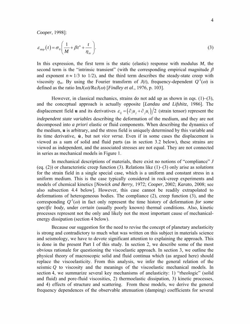
Cooper, 1998]:

0

1 nstep

ss

tt t

M

. (3)

In this expression, the first term is the static (elastic) response with modulus M, the second term is the “intrinsic transient” (with the corresponding empirical magnitude and exponent n 1/3 to 1/2), and the third term describes the steady-state creep with viscosity ss. By using the Fourier transform of J(t), frequency-dependent Q-1() is defined as the ratio ImJ()/ReJ() [Findley et al., 1976, p. 103].

However, in classical mechanics, strains do not add up as shown in eqs. (1)–(3), and the conceptual approach is actually opposite [Landau and Lifshitz, 1986]. The

displacement field u and its derivatives 2ij i j j iu u (strain tensor) represent the

independent state variables describing the deformation of the medium, and they are not decomposed into a priori elastic or fluid components. When describing the dynamics of the medium, u is arbitrary, and the stress field is uniquely determined by this variable and its time derivative, u , but not vice versa. Even if in some cases the displacement is viewed as a sum of solid and fluid parts (as in section 3.2 below), these strains are viewed as independent, and the associated stresses are not equal. They are not connected in series as mechanical models in Figure 1.

In mechanical descriptions of materials, there exist no notions of “compliance” J (eq. (2)) or characteristic creep function (3). Relations like (1)–(3) only arise as solutions for the strain field in a single special case, which is a uniform and constant stress in a uniform medium. This is the case typically considered in rock-creep experiments and models of chemical kinetics [Nowick and Berry, 1972; Cooper, 2002; Karato, 2008; see also subsection 4.4 below]. However, this case cannot be readily extrapolated to deformations of heterogeneous bodies. The compliance (2), creep function (3), and the corresponding Q-1() in fact only represent the time history of deformation for some specific body, under certain (usually poorly known) thermal conditions. Also, kinetic processes represent not the only and likely not the most important cause of mechanical-energy dissipation (section 4 below).

Because our suggestion for the need to revise the concept of planetary anelasticity is strong and contradictory to much what was written on this subject in materials science and seismology, we have to devote significant attention to explaining the approach. This is done in the present Part I of this study. In section 2, we describe some of the most obvious rationale for questioning the viscoelastic approach. In section 3, we outline the physical theory of macroscopic solid and fluid continua which (as argued here) should replace the viscoelasticity. From this analysis, we infer the general relation of the seismic Q to viscosity and the meanings of the viscoelastic mechanical models. In section 4, we summarize several key mechanisms of anelasticity: 1) “rheologic” (solid and fluid) and pore-fluid viscosities, 2) thermoelastic dissipation, 3) kinetic processes, and 4) effects of structure and scattering. From these models, we derive the general frequency dependences of the observable attenuation (damping) coefficients for several

5

physical mechanisms of anelasticity. In sections 5 and 6, we discuss the sensitivity of viscosities (and Q) to pressure and temperature, and suggest a frequency dependence of the attenuation coefficient and Q for a planet.

Our overall conclusion is that the viscoelastic model can should not replace mechanics in application to solid or fluid planets. The classical physical framework [e.g., Landau and Lifshitz, 1986] allows solving seismological and tidal, as well as many other problems. The fading-memory constitutive laws, “intrinsic transients,” frequency-dependent medium parameters, and the “material” Q-factors are therefore not required. Moreover, by abandoning these concepts and using the more general attenuation (damping) coefficients, a simpler, clearer, and physically more consistent picture of mechanical-energy dissipation is obtained. In Part II of this study, we utilize this theory to derive the frequency dependence of tidal Q values for the Earth and Moon.

2 Motivation: viscoelasticity, thermodynamics, and mechanics

In the macroscopic physics of materials, thermodynamics provides the most important guiding principles [Hayden et al., 1965]. Unfortunately, the viscoelastic model incorporates all thermodynamic relations in the empirical time dependences (2) or (3), which makes them not easy to discern. For example, the viscoelastic moduli are conventionally differentiated by the “time scales” of their operation [Nowick and Berry, 1972, p. 8; Jackson et al., 2005]. The “relaxed” modulus, MR, is defined as the one acting at t → , and the “unrelaxed” modulus MU ≥ MR operates at short time scales (t → 0). However, in reality, the difference between these moduli is thermodynamic and not related to the time scales. For deformations conducted at constant temperatures (regardless of their timing), the medium responds with the isothermal modulus, MI (Figure 2). For adiabatic processes (again regardless of how early or late in the process, but with zero heat exchange), the adiabatic modulus MA is in effect. Because of the dissipation of heat, the deformation cycle is irreversible, and therefore MA ≥ MI (Figure 2) [Hayden et al., 1965]. For bulk modulus M K, the ratio of the adiabatic and isothermal moduli depends on the temperature, T, thermal expansion coefficient, , and the specific heat at constant pressure, Cp [Landau and Lifshitz, 1986, p. 15]:

2

1A A

I p

K K T

K C

. (4)

This ratio determines the relative energy dissipation during hysteresis (gray area in Figure 2a).

Apart from its steady-state creep term, the time-dependent (t) in eq. (3) [Gribb and Cooper, 1998] could in principle be entirely thermoelastic, i.e. caused by the temperature T in eq. (4) rapidly rising during stage AB and slowly decreasing during stage BC in Figure 2. Such dissipation occurs even in a perfectly elastic material, and it depends on how the body is thermally insulated during deformation, and also on its shape and thermal conductivity. If kinetic changes, such as diffusion [Gribb and Cooper, 1998], occur within the material under stress, additional terms would also contribute to the KA/KI

6

ratio in eq. (4). In any case, the response of a material to stress is not a function of time but depends on the thermodynamic environment.

Another serious problem in applying the viscoelastic approach to planets consists in its placing zero shear dissipation in liquid zones. For example, in all global Q models of the Earth [e.g., PREM by Dziewonski and Anderson, 1981], shear dissipation within the liquid outer core is set to zero merely because its shear modulus equals zero. Nevertheless, the Earth’s outer core possesses viscosity and substantial shear deformations, and therefore it clearly dissipates the shear energy. This shows that some types of energy dissipation cannot be included in the time-retarded viscoelastic moduli. Two more examples of energy dissipation inconsistent with viscoelasticity are given in Morozov [submitted to AG]. For planetary applications, it is very inconvenient that viscoelasticity only applies to solids and uses so different terminology compared to the mechanics of fluids (Q-1 versus viscosity). Because fluids and solids are intermixed in the compositions of planets, and their mechanical behaviors are similar, it is desirable to find a unified approach to their internal friction. Such an approach is readily supplied by the “physical” model in the following section.

3 Mechanics of anelastic solids and fluids

Classical mechanics is formulated in the time domain, which is already fundamentally different from viscoelasticity. The response of an elastic medium to deformation is described by the functional form of its Lagrangian density, which is a quadratic functional of displacements ui and velocities iu :

,2 2i i kk ll ij ijL u u u u , (5)

where i = 1, 2, or 3 denotes the spatial dimensions, and summations over all pairs of repeated indices are assumed. Parameters and are the Lamé elastic constants, and is the mass density. Most importantly, all medium parameters (, and ) are real-valued and (normally) time-independent. In addition, the density, shear modulus and the bulk modulus 2 3K are non-negative: 0 , 0 , 0K , which makes the kinetic and potential energies in expression (5) real and non-negative for all deformations. By replacing ij with a combination of the dilatational strain, = kk, and deviatoric strain,

3ij ij ij , the Lagrangian density becomes expressed in terms of the bulk and

shear moduli:

2

2 2i i ij ij

KL u u

. (6)

The Lagrangian completely describes the dynamics of the elastic medium. It is most important to see that the mechanical properties of the medium (including its ability to dissipate mechanical energy) are described before any deformations (such as waves) in it are considered. This is another conceptual difference from viscoelasticity, in which energy dissipation and Q are always associated with some kind of an oscillatory or creep

7

process [e.g., Aki and Richards 2002, pp. 162–163].

In order to describe a fluid, we only have to drop the shear-energy part in (6). This can be achieved by setting = 0, as it is usually done. To describe an incompressible fluid, we can also take K , or alternately, drop the 2 2K term as

well but constrain all deformations to the dilatation-free case = 0 (in which case K is replaced with a “Lagrange multiplier”). Thus, in terms of conservative forces, fluids are not significantly different from solids. As shown below, they are also quite similar in terms of the rheologic (viscous friction) and other energy-dissipation laws.

3.1 Dissipation functions as rheologic laws

Energy dissipation is not included in the Lagrangian and is described by another function, D, called the dissipation function or pseudo-potential [Landau and Lifshitz, 1976]. Unlike the potential energy, D principally depends on the strain rates. For small deformations, if we assume a viscous-friction force proportional to the deformation rate, D should be second-order in terms of ij . Because at this point we have no

justification for an internal structure of planetary material similar to the model or porous saturated rock by Biot [1956] or to any of the mechanical models in Figure 1, we construct the dissipation function without internal variables, by generalizing expressions (6). When using only ij in an isotropic medium, the only three rotationally-invariant

second-order scalar functions are 2 , ij ij , and 2 3det . The last of these invariants

still leads to nonlinear equations of motion, and similarly to the case of elasticity, it is not considered here. The generalized dissipation function is therefore constructed by combining the first two invariants:

2

2 ij ijD . (7)

Here, and are the bulk and shear solid viscosities, which were extensively studied for metals [Landau and Lifshitz, 1986]. The same dissipation function applies to fluids [Landau and Lifshitz, 1987], for which parameter is called simply viscosity, or dynamic viscosity, and is called second viscosity and often disregarded for incompressible fluids. For solids, the dissipation function (7) corresponds to the Kelvin-Voigt model (Figure 1b). Jeffreys and Ricker studied its mechanical behavior, which they called “firmoviscous” [see Knopoff and MacDonald, 1958].

Spring-dashpot models of the “linear solids” commonly used in viscoelastic arguments can be viewed as diagrammatic illustrations of the (L, D) pairs above (Figure 1, insets). Note that linear solids often contain “hidden” internal variables, denoted in Figures 1a, c, and d, plus another variable in Burgers model (Figure 1d). These internal variables are responsible for the “realistic” behaviors of such models, such as plastic flows and the time delays in developing the “relaxed” elastic moduli. Because these internal variables are considered massless (no kinetic-energy terms 2 2m in the Lagrangians; insets in Figure 1), they instantly respond to the external stress rates applied

8

to the whole bodies and are excluded from the equations of motion. However, the assumption of zero mass is not very realistic, and detailed physical models [e.g., Biot, 1956] show that internal variables usually have inertial effects associated with them.

The diagrams in Figure 1 also explain the (apparent) dilemma about whether Q-1 should be correlated or anti-correlated with viscosity, as mentioned in the Introduction. For viscoelastic solids (Figures 1a, c, and d), the elastic limit is usually obtained by making the viscosity high: , and this is also the empirical association made in seismology [Anderson, 1965; Sato, 1991]. However, in fluid- and solid-state mechanics, viscosity is a measure of energy dissipation, and the elastic limit is 0 (Figure 1b). This difference is due to the internal variables in the viscoelastic solids. Viscosity in a Maxwell, Zener (standard linear), or Burgers solids (Figure 1a, c, and d, respectively) is analogous to the pore-fluid viscosity (see subsection 4.2) and is not the viscosity encountered when the rock flows as a whole. An increase of in Figures 1a, c, and d “freezes” the internal variables, and the body becomes elastic. By contrast, viscosity in a Voigt body (Figure 1b), and also and in eq. (7) are the solid/fluid viscosities experienced in a whole-rock flow. These viscosities are meaningful for tidal and seismic deformations and can be compared to the viscosities measured from very slow (e.g., glacial rebound or tectonic) flows of mantle rock. It is straightforward to show [e.g., Morozov, submitted to AG], that the inverse Q-factor, for example, of an S wave in such a medium is proportional to viscosity:

1SQ

, (8)

where is the shear modulus and is the circular frequency.

From geodynamic and lab studies [e.g., Karato, 2008], it is known that Newtonian viscous friction (7) is not appropriate for the Earth’s and presumably other planetary mantles. In rocks, friction forces appear to be increasing slower than the strain rate. To account for this observation, we introduce exponents and k into (7):

2

2 22

1

2 r ij ij rr

D

. (9)

With such D, the frictional stress associated, for example, with dilatational deformation is:

122

2 r

D

, (10)

which is proportional to for Newtonian fluid ( = 1) and constant for dry (Coulomb) friction ( = 0.5). A time-scale parameter r is required in this equation in order to maintain the correct dimensionality of D. However, this parameter can be absorbed by the measurement units for and selected by convention (for example, equal 1 s).

9

Analysis of the Earth’s free oscillations [Morozov, unpublished] suggest that in its crust and mantle, the values of range from 0.5 to 0.63, and so they are close to “dry” rheologies.

3.2 Unified solid-fluid rheology

Rocks behave nearly elastically under certain conditions, and under some other conditions they flow. Conventionally, such conditions are specified by the differences in the time scales of deformations [e.g., Turcotte and Schubert, 2002; Jackson et al., 2005]. This point of view is inspired by the observation that most Earth’s materials become more “fluid-like” after stress is applied for an extended time. This is illustrated in Figure 3, in which the “flowing” rocks occupy the lower-right part of the diagram, where the characteristic time scales of deformations increase. However, such a view may only be apparent. Time-variant material properties are actually not required, and the same elastic-to-plastic transition can be explained simply by strains exceeding the level of 0 ≈ 10-4–10-3 (Figure 3). This suggests that a nonlinear rheology can naturally explain the apparent “time-scale” dependence of material properties. The fact that materials indeed behave non-linearly at strains ~0 is quite clear from lab studies. At such strains, the elastic energy is comparable to the energy of bonds between mineral grains, and rocks start fracturing and “flowing” when larger volumes are considered.

3.2.1 Conservative part (Lagrangian)

If a material exhibits plastic creep with a “viscoelastic” transient (as in eq. (3)), it can be described by decomposing the displacement vector into “solid” and “fluid” parts:

s f u u u , similarly to eq. (1). For example, us could consist in the deformation of solid

blocks of rock (for example, of its grains), and uf – in relative movements of these blocks. Then, the Lagrangians (6) would only apply to us, and for uf, there would be no elastic-energy terms (i.e., Kf = f 0):

2, , , , , , , , ,2 2 2

fs ss i s i s s ij s ij f i f i sf ij s i f j

KL u u u u u u

, (11)

where additional subscripts s and f correspond to the solid and fluid parts of the displacement, respectively.

In general, recognition of the two variables us and uf, leads to two additional complications of the kinetic-energy terms in (6): 1) the values of density in them may be different: f ≠ s, and 2) the total kinetic energy may contain cross-terms (with sf in (11)), which intermix the velocities su and fu . Generally, the description would be

similar to the saturated porous rock model described in subsection 4.2. Fortunately, in cases of practical importance, the deformations are either 1) near-elastic (for oscillations), for which we can likely disregard uf compared to us, or 2) very slow (for creep and tectonic movements), in which case the entire kinetic energy is negligible, and

s fu u . Thus, it appears that f and sf in (11) should be insignificant in all practical

10

cases, and the conservative part of the mechanical model is simply determined by the solid density and elastic moduli (6).

3.2.2 Dissipation (rheologic) part

The strain dependence of rheology can be incorporated in the nonlinear dissipation function (9) in several ways. For example, the following functional form of D appears to account for the observed strains and strain rates of deformations within the Earth (Figure 3):

s fD D D , (12)

where the dissipation functions for “solid” and “fluid” deformations are:

,

,2 2

, ,, ,2 2, ,2 2 2 2

0 02

s

ss ij s ijs ss ss r r s ij s ij

r r

D

, and (12a)

,

,

2, ,2 2

, ,2 22

f

ff f ff r r f ij f ij

r r

D

. (12b)

A detailed discussion of the effects of rheology (12) on the interpretation of observations is done in Part II. As shown there, exponents for solid and fluid deformations can be taken approximately equal. Note that in Ds, we also introduce a power-law dependence on strain. By taking 0 ≈ 10-4, ≈ 0.47, s, ≈ 0, s, equal ~0.6 and 1.0 within the Earth mantle and core, respectively, dissipation function (12) quantitatively reconciles the glacial-rebound, tidal, free-oscillation, broad-band seismic, and lab creep observations for the Earth. Note that it turns out that within the crust and mantle, s, + ≈ 1, which means that the dissipation functions scales with as approximately 2D . Therefore, for low strains, energy dissipation within the Earth is nearly independent of strain amplitudes. However, this observation may change for the Moon or other planets.

3.3 Elastic and viscous stresses

Once the functional forms for L and D are selected, the dynamics of the system becomes completely described. Elastic stresses within a deformed body are given by

ijij

L

, and frictional stresses are:

D D

for dilatational, and D

ijij

D

for deviatoric deformations. (13)

Note that in the viscoelastic model, such elastic and frictional stresses are both included in the “viscoelastic” stress and cannot be separated. In consequence, the strain energy is non-unique in viscoelasticity [see section 2.1 in Carcione, 2007].

11

From (13), the dissipated power per unit volume equals

ij ijij ij

D D DP

. (14)

This mechanical power dissipated by friction is associated with the “rheologic” mechanism of anelasticity in section 4. In addition, several non-mechanical energy-dissipation mechanisms add up to P. These mechanisms are also discussed in section 4.

3.4 The Q’s

As shown in section 4, in all physical models, the inverse Q-factor arises as a ratio of the temporal attenuation coefficient () to the frequency of the selected oscillation ():

1 2Q

. (15)

This Q-1 is an apparent (observable) property of the wave. Similarly to , this is also the temporal Q-1 [Aki and Richards, 2002]. For a traveling wave, spatial Q-1 can be defined similarly:

1 2spatialQ

k

, (16)

where k is the wavenumber and is the spatial attenuation coefficient [Morozov, 2010]. Expressions (15) and (16) also show that and represent the primary attributes of attenuation, to which we need to devote most attention.

4 Mechanisms of mechanical-energy dissipation

In this section, we outline four groups of physical processes causing mechanical-energy dissipation: 1) solid and pore-fluid viscosity, 2) thermoelasticity, 3) kinetic processes, and 4) scattering and the effects of structure. Only the first of these groups is a purely mechanical process, which represents a stress to strain-rate relation and can therefore be associated with a “rheologic law.” In addition to viscosity, many non-mechanical processes also dissipate mechanical energy. Strictly speaking, they should not be called “rheologic,” because the stresses produced by them are generally dissimilar to viscous friction and not related to the strain rates. Among such processes, the distinctive characteristic of thermoelasticity is the importance of thermal expansion and temperature anomalies spreading in space. A broad group of “kinetic processes” includes various types of transformations taking place within the local microscopic structure of a material occurring under stress. Such processes receive the most attention in viscoelasticity [Nowick and Berry, 1972; Karato and Spetzler, 1991; Cooper, 2002]. Finally, the distinctive feature of scattering consists in elastic dissipation, i.e., mechanical energy being conserved but redistributed in space and time.

12

In the following, many details and illustrations are left aside, and our principal goal consists in explaining the characteristic frequency dependencies of and Q-1 for each group of dissipation processes, as summarized in Figure 4. Note that for each of these processes, there exists a characteristic relaxation time 1

r . Consequently, if not

looking at their physical differences and spatial variations, and staying limited to a certain oscillation type, these processes can be (somewhat loosely) treated as viscoelastic “relaxation mechanisms” [Liu et al., 1976].

4.1 “Rheologic” solid and fluid viscosity

Rheologic equations for a fluid flow are usually written as giving the stationary strain rate, , resulting from a quasi-static stress, . This relation is often taken in the power-law form: n [Karato, 2008]. In more detail including the dependence on pressure (p) and temperature (T), the rheologic relation for plastic creep is [Karato and Wu, 1993]:

expn m

a aE pVbA

h RT

, (17)

where A is some pre-exponential factor, is the shear modulus, h is the grain size, b is the lattice spacing, Ea is the activation energy, Va is the activation volume, and R is the Boltzmann’s constant. Exponent n ranges from about 1 for dislocation creep to ~3.5 for diffusion creep [Karato and Wu, 1993].

As mentioned in the Introduction, from the viewpoint of fluid- or solid-continuum mechanics [section 3; Landau and Lifshitz, 1986], eq. (17) represents not a constitutive law but its inverse, i.e. a solution for a stationary flow under some boundary conditions. To describe the viscosity of the medium itself, we need to write the dissipation function D, from which the frictional stress is derived, as in eqs. (12) and (13). Thus, the dissipation function plays the role of the rheologic law. The above dependence

1 n arises from the power-law form of the dissipation function (9) and (12), which gives 2 1 for each of the two types of deformation (bulk and shear). For values of n from 1 to 3.5, exponents 1 1 2n vary from 1 to ~0.65, respectively. For a fixed

deformation amplitude and variable frequencies, ij , and the attenuation (damping)

coefficient for volume V of a wave is:

2

222

ijijmech V

mechij ij

V

D

E

E

(18)

for both bulk and shear deformations in D, where the overbars indicate the quantities averaged over a period of oscillation, and angular brackets

V are the volume averages.

In Figure 4a, such dependences are shown for = 0.5 and 1, and the corresponding

13

1 2Q are shown in Figure 4b.

4.2 Pore-fluid viscosity

Another instructive and well-developed example is the case of fluid-saturated porous medium. In this case, at least a two-phase medium, such as porous rock saturated with fluid, is required. By relative movements of the two phases, mechanical energy is dissipated, and various kinematic and dynamic effects are produced. We only briefly outline the general sense of this theory here, following Bourbié et al. [1987, p. 69–81].

In Biot’s [1956] theory, the dimensions of the macroscopic elementary volumes are assumed to be small compared to the wavelength, and the deformation is weak. It is therefore sufficient to consider only quadratic terms in the volumetric density of the kinetic energy:

2 2u w

k i i i i uw i iE u u w w u w , (19)

where w U u is the “filtration” velocity of the fluid U relative to the rock matrix u . The kinetic matrix-fluid coupling parameters above are determined by the porosity and permeability of the rock. For example, u in this expression is the average density:

1u s f , (20)

where s and f are the densities of the matrix and fluid, respectively, and is the porosity.

Similarly to Ek, the poroelastic dissipation function is also taken to be quadratic in filtration velocity:

2 i iD w w

, (21)

where is the fluid viscosity, and is the absolute permeability, which depends on the geometry of the pores among other factors. For P waves, the displacements of rock matrix and fluid can be expressed through the corresponding scalar potentials 1 and 2, which can be combined in a two-component vector field,

1

2

uΦ

U

, (22)

where

denotes the spatial gradient operator. The Euler-Lagrange equations in respect to are:

2 0 R Φ AΦ MΦ , (23)

14

where R and M are the rigidity and mass matrices, respectively,

2

2 2f M M

M M

R , (24)

2 1

1f f

f f

a a

a a

M , (25)

and A is the damping matrix:

b b

b b

A . (26)

In these expressions, f is the second Lamé modulus of a closed system (i.e., the modulus corresponding to the case of fluid content being constant). Parameter M has the meaning of pressure that needs to be exerted on the fluid in order to increase the fluid content by a unit value at iso-volumetric conditions (kk = 0). Parameter b is defined as b = 2/ where is the hydraulic permeability, or mobility of the fluid within the rock. Parameter [0,1] quantifies the proportion of the apparent macroscopic volumetric strain caused by the variations in fluid content, which can be illustrated by the expression of the strain-stress relation:

2 2ij f kk ij ij ijM p , (27)

where p is the mean fluid pressure.

In the absence of mechanical-energy dissipation (e.g., for = 0 or = 0), matrix 1R M in (23) is positive definite and symmetric, and consequently it has two real

positive eigenvalues. These eigenvalues are the squares of the two P-wave velocities, 2,1PV and 2

,2PV . The corresponding eigenfunctions have the forms of plane waves with

wavenumbers equal /VP,1 and /VP,2, respectively. In the presence of energy dissipation, these wavenumbers become complex, and their imaginary parts (attenuation coefficients) can be expressed through the normalized functions BP for both the slow and fast

P waves:

B

BP

PV

, (28)

and a similar expression for S waves. Functions BP and BS were

tabulated for different combinations of parameters by Bourbié et al. [1987, pp.76–78]. Note the Biot’s reference frequency B, which depends on the filtering medium:

15

Bf

. (29)

Bourbié et al. [1987, p.79] noted that B can be extremely variable, ranging from 30 kHz to 1 GHz for water. Nevertheless, B is always quite high, and both tidal and seismic frequencies are located deep in the low-frequency limit for poroelastic relaxation. With increasing frequencies, both attenuation and phase velocities monotonously increase, approximately as 2 (Figure 4).

4.3 Thermoelastic dissipation

Thermoelastic effects are pervasive, and they represent the most common cause of anelasticity in materials [Hayden et al., 1965; Landau and Lifshitz, 1986]. On the Moon, thermoelasticity could be the principal reason for its unusual seismic and tidal attenuation properties [Nakamura and Koyama, 1982], and as we argue in Part II, it may also be very important for the Earth and other planets. Thermoelastic effects result from the variations of material’s volume or pressure during deformation, which cause variations in its temperature, T. Spatial variations in T further lead to heat fluxes, q, within and outside the body:

i iq T . (30)

where is the thermal conductivity of the material. For an isotropic body, the total mechanical energy-dissipation rate by heat conduction is proportional to the average squared gradient of the temperature [see Landau and Lifshitz, 1987, §79]:

2

mechE T dVT

. (31)

The temperature variation can be derived from the adiabatic approximation for entropy [Landau and Lifshitz, 1986, §6]:

0S T S T K , (32)

where is the dilatational strain, S0 is the entropy in the absence of deformation, K is the isothermal bulk modulus, and is the thermal expansion coefficient at constant pressure:

1

p

V

V T

, (33)

where V is the volume. The isothermal modulus K in (32) is related to the adiabatic modulus Kad as:

adV

p

CK K

C , (34)

where Cp is the specific heat at constant pressure, and Kad can be inferred from seismic

16

wave velocities (VP and VS) and density :

2 2ad

4

3P SK V V

. (35)

Therefore, the temperature variation within an adiabatically (for example, very quickly) deformed medium is proportional to the dilatational strain (Figure 2):

0 ad0

p

T KT T T

C

. (36)

For a typical rock, this gives roughly 00.4T T . Combining the above relations

shows that heat conduction causes energy dissipation at the following rate [Landau and Lifshitz, 1986]:

2

admech

p

KE T dV

C

. (37)

Thus, mechanical energy is actively dissipated in areas of high dilatational strain (, and also within zones of strong variations in material properties (VP, VS, , , or Cp).

From eq. (37), only dilatational deformations with ≠ 0 lead to thermoelastic dissipation. However, for shear deformations in grainy, polycrystalline materials, mechanical contrasts between the grains cause highly heterogeneous, anisotropic deformations of the grains. As a result, dilatational deformations always exist at the grain-size scale, and consequently shear waves within rocks should also exhibit thermoelastic dissipation [Armstrong, 1980].

Thermoelastic dissipation shows complex dependences on frequency, depending on the relations between the frequency , grain size h, wave speed c, and thermometric conductivity C (Figure 4a). For Newtonian viscosity ( = 1) within the grains (“crystallites”), three regimes of thermal relaxation in polycrystalline bodies are recognized [Armstrong, 1980; Landau and Lifshitz, 1986, pp. 139–140]:

1) For very low frequencies 2h , crystallites equilibrate within each period of oscillation, and the oscillation occurs nearly isothermally (Figure 2). In this case, 2 , similarly to the case of linear viscosity. The effective value of viscosity is much higher than that of the individual crystallites (Figure 4a).

2) For frequencies 2h c h , thermal equilibration takes place by means of “temperature waves” across the boundaries of crystallites. This process is similar to the skin effect in electromagnetism. Only a small portion of the volume is involved in relaxation, and consequently the corresponding (Figure 4a).

17

3) For c h , the wavelengths are much shorter than the dimensions of the crystallites, and the deformations are nearly adiabatic (Figure 2). The resulting thermoelastic dissipation is again similar to Newtonian viscosity, with 2 (Figure 4a).

Similar regimes should clearly exist for our nonlinear rheologic laws (9) and (12).

Thermoelastic relaxation times lie within the common periods of seismic and tidal deformations. It is easy to estimate (even from dimensionality considerations) that a spatial variation in temperature of size a would dissipate over time

22 24p pC C

ak

, (38)

where 2k a is the characteristic wavenumber of perturbation. For a typical rock,

2800 kg/m3, Cp 800 J/kg/K and 2–7 W/m/K, and therefore (8000–30,000)a2 in SI units. Consequently, for seismic periods of 1 s, thermoelastic perturbation sizes should be a 0.5–1 cm. This a is close to the scale-length of layering commonly found in crustal sedimentary sequences, and also to the dimensions of laboratory devices in which material properties are usually measured. For tidal deformations of the Earth ( 4.3105 s), a 3–6 m, and for 2.6106 s (one-month lunar tide), a 8–16 m, which is also reasonable for crustal heterogeneity. These scales show that the crustal and mantle structure is an important factor for thermoelastic dissipation. Note that all of these scales are much larger than grain sizes usually considered in microstructural interpretations of anelasticity [Karato and Spetzler, 1991].

4.4 Kinetic processes

A broad range of non-mechanical processes of energy dissipation can be described by internal variables [Chapter 5 in Nowick and Berry, 1972; also see Figures 1a and c]. Such variables are used to describe certain types of internal changes within the material that give rise to anelasticity. Examples of such variables include squirt flow densities, concentrations of point dislocations or defects within the crystalline lattice, ionic or chemical concentrations, spin orientations, and other. For simplicity, let us consider a single internal variable, denoted . In terms of its effect on the mechanical system, assume that a variation of the vector of causes the mechanical energy to dissipate at a certain rate:

mechdE

dt ξ . (39)

Function may also depend on mechanical parameters of the system, temperature and other factors.

The dynamics of internal variables is described by kinetic equations, which are similar to the equation of diffusion [Nowick and Berry, 1972; Cooper 2002]. The internal

18

variables are assumed to possess some equilibrium levels, designated , which depend on the strain and stress within the body, as well as on its temperature. The kinetic equation is then:

1d

dt

. (40)

For a fixed (such as in a static creep), the kinetic variable exponentially approaches its

equilibrium value after a “relaxation time” :

expt

A

. (41)

For a harmonic process at frequency (such as a seismic wave), the internal parameter is coupled to the mechanical state of the system, and therefore the “equilibrium level” oscillates as:

0 i tt e . (42)

The first of these terms again gives the relaxation law (41), which is insignificant if only stationary oscillations are considered. The second term in (42) leads to an oscillation of , which is phase-delayed relative to :

i te , where1 i

. (43)

For this general example, it appears reasonable to take the dissipated power as a function of the amplitude of , i.e. of . Let us consider a power-law dependence:

221

, and

1

122

1Q

. (44)

In Figure 4, such dependences are illustrated for = 2, which corresponds to kinetic processes considered by Nowick and Berry [1972]. Note that similarly to thermoelastic relaxation, kinetic processes exhibit absorption peaks in Q-1 (Figure 4b).

4.5 Effects of structure and scattering

The effects of structure and scattering on mechanical-energy dissipation represent an extensive subject discussed in Morozov [2008, 2009a, b, 2010, 2011a, b]. Here, we only summarize some key points of these arguments. Scattering on small random heterogeneities is both practically and theoretically indistinguishable from the uncertainty of the “background model” (such as the geometrical spreading or reflectivity) in an

19

imperfectly-known structure. Therefore, the best approach is to treat them together, by using the empirical temporal attenuation coefficient, . Depending on the structure (e.g., spherical or near-surface layering), the dependence of on frequency can be very general. However, analysis of many datasets for the Earth shows that within typical data errors, near-linear () dependences are often observed:

2 eQ

. (45)

In this expression, is interpreted is the “geometrical attenuation,” and the dimensionless parameter Qe is the “effective quality factor.” Notably, is positive for most crustal datasets and correlates with tectonic types of the crust. It can also be predicted from theoretical models of random reflectivity or ray bending [Morozov, 2011c] and from numerical seismic waveform synthetics [Morozov et al., 2008]. Positive values could also be responsible for the commonly observed decrease of the apparent Q-1 with frequency:

1 12 11e

r

Q Q

. (46)

where 2r eQ is the characteristic “relaxation time” for geometrical effects.

Scattering represents an “elastic attenuation,” which means that it does not reduce the total amount of mechanical energy in a closed system. In application to planetary deformations, it may therefore appear that scattering should not affect the phase lags between the torque caused by an orbiting satellite and the resulting tidal deformation. However, elastic scattering should in fact affect the tidal bulge, which can be shown as follows. The deformation of a planet can be represented by a sum of spherical harmonics,

, ,nlmY r :

, , , ,nlm nlmnlm

u r c Y r . (47)

Only a few of the lowest-order harmonics are available for seismological and tidal observations, whereas the entire spectrum of high-frequency modes is very rich and incorporates all high-frequency body and surface waves. In a radially-symmetric planet, harmonics with different l, or m do not interact and oscillate with their own natural frequencies, nl . However, in a heterogeneous planet, all harmonics interact by means of

the non-zero cross-terms in the Lagrangian (5):

2; , , , , , ,n l m nlm n l m nlmK p r Y r Y r r drd d , (48)

where p is some material property, such as , , or . In the state of thermodynamic equilibrium, these harmonics are distributed according to the (canonical) Gibbs distribution [Landau and Lifshitz, 1980]:

20

exp nlmnlm

Ew A

T

, (49)

where wnlm is the probability to find the system in state (n,l,m), T is the temperature, and A is some normalization constant. This shows that although weak, high-frequency modes are always present in the state of equilibrium.

An external force, such as the tidal potential created by an orbiting satellite, acts on some modes preferentially (n, l = 0, 2 for tides [Agnew, 2009]) and brings them above the equilibrium level. As a result, modes Y02m begin to “diffuse” into the higher-order modes, according to the Boltzmann’s transport equation [Lifshitz and Pitaevskii, 1981]:

dwC w

dt , (50)

where C(w) is the “collision integral,” which in our case describes the interaction of a given mode with all other modes. For the mode amplified by the external field, C(w) < 0, whereas for most high-order modes, C(w) > 0. Thus, although the total energy is preserved, it is removed from modes Y02m into the higher-order modes and lost for the observation. The spectral line for modes Y02m should therefore broaden by the amount of dissipation C w ( > 0), and the corresponding phase lag appears between the

orbital torque and tidal deformation.

The frequency-independent geometrical attenuation appears to be the most important part of seismic-wave energy dissipation found in most datasets (note that it is also disregarded by the conventional parameterization 2Q , which implies that

0 for 0). Such = = const with the corresponding Q-1 from eq. (46) are shown in Figure 4. Note that similarly to kinetic and thermoelastic processes, scattering and structure can account for the observed “high-frequency background,” with 1Q

approximately proportional to .

5 Dependence on temperature and pressure

The dependence of mechanical-energy dissipation on pressure and temperature is a very interesting subject requiring extensive analysis. If viewing solid viscosity as the common cause of internal friction, an apparent controversy between the (p,T)-dependences of the near-elastic and plastic deformations is revealed. As suggested by expression (17), for strong (fluid-like) deformations 0 , viscosities and in (12)

increase with p and decrease with T as [Karato and Wu, 1993]:

expm

na aE pVb

h nRT

. (51)

Such dependence (p,T) is typical for fluids. However, for near-elastic deformations, the following empirical dependence was proposed from global Q models and lab measurements [Sato, 1991]:

21

1

00

1exp 1m

m

TQ g

pV TQRT

, (52)

where Q0, V0, and g are some constants, and Tm is the melting temperature. Considering that generally 1Q , this dependence on (p, T) is opposite to (51) and suggests that viscosity increases with temperature and decreases with pressure. From similar observations, Anderson [1965], Sato [1991], and other authors inferred that it is the Q but not Q-1 that should correlate with viscosity.

Nevertheless, from first principles (section 3), the dissipation (Q-1) should still be directly related to viscosity. The solution to this controversy is that for near-elastic deformations ( 0 ), solid viscosities in (12) do indeed increase with temperature.

Generally, this could be because of the nearly “dry” character of internal friction, corresponding to 0.5 in our dissipation functions (9) and (12) (more detail on this given in Part II) and nearly frequency-independent Q for seismic waves [Knopoff and MacDonald, 1958]. For dry friction, the actual deformation (slip) likely occurs along a small portion of grain boundaries, with the rest of them being locked by static friction, adhesion, mineralization, etc. Therefore, the volume V within which the mechanical energy is dissipated in eq. (18) likely represents only a small portion of the total volume. This volume could be similar to the volume affected by “unpinning” of dislocations [Karato and Spetzler, 1990]. With increasing temperature and decreasing pressure, this volume should increase, similarly to what is shown by eq. (52). In such a way, “dry-solid” viscosity is a thermally-activated process, and both and 1Q for seismic-scale (weak) deformations increase with mantle temperatures and decrease with pressures. In terms of our rheologic law (12), this behavior can be described by the elastic-to-plastic transition strain threshold, 0, decreasing with T and increasing with p. For the same reason, the effective viscosity should likely decrease with increasing relative lattice spacing b/h, as shown in expression (51).

Thermoelastic dissipation also quickly increases with temperature (see eq. (37) in subsection 4.3). In heterogeneous near-elastic bodies, its effect is roughly similar to that of viscosity, and it therefore contributes to the noted increase of solid viscosity with temperature.

6 Frequency dependence

The phenomenon of frequency dependence of Q receives much attention and is often viewed as the primary source of information about the rheology in Earth-materials science [Karato, 2008], geodesy [e.g., Efroimsky and Laney, 2007] and seismology [e.g., Romanowicz and Mitchell, 2009]. In these contexts, the frequency-dependent Q is viewed as a key material property. However, in our interpretation, the primary quantities are and (subsection 3.4), and therefore we only need to examine their frequency dependences for planetary oscillations and seismic waves.

Two general causes for and varying with frequency can be recognized: (I)

22

combination of physical processes of mechanical-energy dissipation discussed in section 4, and (II) measurement artifacts. The second of these alternatives refers to using different wave types, or utilizing temporal, spatial, phase-lag, or near-resonance observations and different corrections for the “elastic” background, such as selection of the geometrical-spreading exponent. This can lead to a variety of frequency dependences (particularly for Q), which may be difficult to compare but nevertheless artificial [Morozov, 2008, 2010].

Let us now assume that factor (II) is leveled by using some consistent measurement procedures, and focus on the physical factors (I) using the results of section 4. Note that for all types of energy dissipation, the attenuation coefficient increases with frequency (Figure 4a). Thermoelastic processes and kinetic phenomena often show bands of increased Q-1 near frequencies = -1, where are the characteristic relaxation times (Figure 4b). A broad ”absorption band” was inferred for mantle and crustal materials [Anderson et al., 1977], and its upper flank is called the “high frequency background” in materials science [Cooper, 2002]. Scattering and structural effects can also produce similar patterns of Q-1 rapidly decreasing with frequency (Figure 4b). However, once again, note that such dependences of and Q-1 on only relate to the apparent quality factors for certain oscillations, and should not be attributed to the material.

Combinations of the () dependences in Figure 4a produce the observed energy-dissipation properties for bodies and oscillation modes. For example, for tidal deformations of a planet, () should be:

2 2 2 2struct struct dry dry wet wet kin kin

2

2adthermo ,W

p

a a a a

K

C

W W W W

(53)

where W is the amplitude of the corresponding free oscillation (principally, the fundamental spheroidal mode with l = 2), W is the dilatational strain in this mode, Kad is the adiabatic bulk modulus, is the thermal expansion coefficient and Cp is the specific heat at constant pressure, and brackets ... denote spatial averages. Contributions of the

different factors denoted ‘a’ are determined by the distributions of physical properties within the planet. For the Earth, along with the general effect of the spheroidal geometry, astruct is likely dominated by the crust and upper mantle, adry comes from the upper mantle (with ≈ 0.63) and lower mantle (with ≈ 0.5), and awet appears appropriate for the outer and inner cores, in which ≈ 1 [estimates for from Morozov, unpublished]. The contribution from thermo is proportional to the squared gradients of physical properties, which should be strong near major boundaries and within heterogeneous zones, such as the crust. These models are discussed in detail in Part II.

If desired, the for the free-oscillation mode (53) can be converted into a tidal phase lag tan = 2/ and also into a phenomenological time-domain response to a step-

23

function torque, which will likely be close to the Andrade [1910] law (3). For each dissipation type in (53), its time-domain response can be further transformed into a frequency dependence of Q-1. These transformations are also illustrated in Part II. However, such Q-1() models seem to offer few additional insights into the behavior of the planetary body while obscuring the physical meaning of the basic equation (53).

7 Discussion

The physical models presented in this paper are very difficult to reconcile with the (now) traditional notions of “material memory” or “intrinsic transient.” As shown in Morozov [submitted to AG], the effects of material memory can in principle be produced by attributing internal (kinetic) variables to the material (as in Figure 1), and yet their introduction is artificial and contradicts certain very basic physical observations. At the same time, all of the physical mechanisms described in section 4 neither require nor lead to a material memory.

The difference of the theory presented here from viscoelasticity can be clearly illustrated on the following summary of the viscoelastic model by Cooper [2002]: “It is useful to consider inelastic responses as the relaxation of elastic strain energy: with the application of stress, elastic energy is stored into the material <…> instantaneously; inelastic, time-dependent relaxation can occur, assuming the applied stress is sustained for sufficient time <emphases ours – I.M.>.” Thus, the viscoelastic model assumes that 1) it is the elastic energy that is stored and then dissipated, and 2) that the dissipation is controlled by time. However, as shown in section 4, the elastic energy is only a part of the total mechanical energy, and there exists no reason to believe that only this part is dissipated. All dissipation processes in section 4 are quite unlike the elasticity. Also, if the relaxation takes place in the form of heat exchange or diffusion, it should occur by spatial flows and not as local variations with time. The relaxation should also depend on how such flows are maintained (for example, influenced by the shape of the body).

Kinetic processes form the principal theoretical support for the phenomenon of material memory [Nowick and Berry, 1972; Karato and Spetzler, 1990; Cooper, 2002]. Indeed, such processes (subsection 4.4) occur locally and are presented as time-delayed responses at the individual points within the medium. Nevertheless, an important subtlety seems to be often overlooked in this argument. In order to dissipate mechanical energy, the process of deformation must be thermodynamically irreversible. Because during oscillations (for example, tidal or seismic), the medium periodically passes through identical states (and does not, for example, fracture or gradually change its chemical composition), the only irreversible change in it is related to the generation and absorption of heat. Therefore, kinetic processes should again be not local, “memory” processes but depend on the spatial flows of heat (subsection 4.3). If heat flows are prevented, or conversely, encouraged by controlling the temperature of the body, kinetic processes may proceed differently.

Once starting to look for the specific physical factors (instead of a Q) controlling the attenuation of oscillations in planetary bodies, we realize that they are poorly understood at present. For metals (and therefore possibly metal cores of some planets), several important results were given by Landau and Lifshitz [1986]. Armstrong [1980]

24

applied these results to explaining the near-constant Q() in sedimentary rocks. For an isotropic, porous, fluid-saturated rock, Biot’s [1956] framework presented numerous insights, which were extended, for example, to Rayleigh waves by Deresiewicz [1960] and to cases of more complex porosities by Beskos et al. [1989]. For recent reviews of poroelasticity, see Müller et al. [2010] and Singh [2011]. However, for rocks at deep crustal, mantle and whole-planet conditions, physical mechanisms of energy dissipation remain unclear.

As shown in section 4, the apparent attenuation coefficients and provide a good basis for both theoretical and experimental analysis of planetary anelasticity. Different physical mechanisms of anelasticity produce characteristic dependencies of and on frequency. Thus, if we measure, model, and invert for and/or directly, and use the specific models of anelasticity instead of the “blanket” Q, significant physical parameters of the medium become constrained. In Part II, this analysis is carried out for terrestrial and lunar tides.

8 Conclusions

The broadly used viscoelastic model of anelasticity in Earth and planetary materials represents only a phenomenological approximation to the full physical description. Here, such a physical model of tidal and seismic-wave attenuation is outlined. Instead of the “blanket” in situ Q, several mechanisms of mechanical-energy dissipation are recognized: 1) solid and pore-fluid viscosity, 2) thermoelastic effects, 3) various kinetic processes within the material, and 4) structural and scattering effects. The group of viscosity mechanisms 1) is associated with rheologic laws and described by Lagrangian dissipation functions. A unified rheologic relation is proposed, which combines the near-elastic and plastic deformations. Instead of the conventional assumption of rock properties varying with the time scales of stress application, this relation explains the elastic-to plastic transition by the nonlinearity of the dissipation function in respect to both the strains and strain rates. For the Earth’s crust and mantle, this nonlinearity appears to be weak for strains but strong (close to dry-friction type) for strain rates. Because of the interpreted dry friction, solid viscosity increases with temperature and decreases with pressure for near-elastic deformations but behaves oppositely for plastic deformations. This can be explained by the elastic-to-plastic transition strain level, 0, decreasing with temperature and increasing with pressure.

Different dissipation processes and types of oscillations lead to characteristic frequency dependences of the temporal attenuation (damping) coefficient, . Solid viscosity leads to 2 and the apparent 1 2 1Q , where is the rheologic exponent, which is near one for fluids and equal 0.5–0.63 for the Earth’s mantle. For pore-fluid viscosity, these parameters scale approximately as 2 and 1Q . Notably, the thermoelastic and kinetic processes lead to absorption peaks in the apparent Q-1. Scattering is also likely to contribute to the well-known “high-frequency background” of Q-1 decreasing with frequency.

25

Acknowledgments

This paper was started during author’s sabbatical visit at the Air Force Research Laboratory, Hanscom Air Force Base, MA, sponsored by the U.S. National Research Council. I thank Dr. Anton Dainty for hosting this visit. I also thank Bob Nowack and Michael Efroimsky for numerous discussions of anelasticity.

26

References Agnew, D. C. (2009), Earth tides, in: Romanowicz, B., and A. Dziewonski (Eds.), Treatise on Geophysics,

v. 3, Geodesy, ISBN 978-0-444-53460-6, p. 163–195. Aki, K. and P. G. Richards (2002), Quantitative Seismology, Second Ed., University Science Books,

Sausalito, California. Anderson, D. L. (1965), Earth’s viscosity, Science, 151, 321–322. Anderson, D. L., H. Kanamori, R. S. Hart, and H.-P. Liu (1977), The Earth as a seismic absorption band,

Science, 196 (4294), 1104 – 1106. Andrade, E. N. da C. (1910), On the viscous flow in metals, and allied phenomena, Proc. R. Soc. Lond. A,

84, 1–12 Armstrong, B. H., 1980. Frequency-independent background internal friction in heterogeneous solids,

Geophysics 1042–1054. Beskos D. E., C. N. Papadakis, and H. S. Woo (1989), Dynamics of saturated rocks. III: Rayleigh waves, J.

Engrg. Mech., 115, 1017–1034. Biot, M.A. (1956), Theory of propagation of elastic waves in a fluid-saturated porous solid. J. Acoust. Soc.

Am. 28, (a) 168–178, (b) 179–191. Bourbié, T., O. Coussy, and B. Zinsiger, (1987), Acoustics of porous media. Editions TECHNIP, France,

ISBN 2710805168. Carcione, J.M. (2007), Wave fields in real media: Wave propagation in anisotropic anelastic, porous, and

electromagnetic media, Second Edition, Elsevier, Amsterdam. Cooper, R. (2002), Seismic wave attenuation: Energy dissipation in viscoelastic crystalline solids, in: S.-I,

Karato and H. R. Wenk (Eds.), Plastic deformation of minerals and rocks, Rev. Mineral Geochem., 51, 253–290.

Cormier, V.F. (2011), Seismic viscoelastic attenuation, in: Gupta, H. K. (Ed.), Encyclopaedia of Solid Earth Geophysics: Springer, doi: 10.1007/978-90-481-8702-7, 1279–1289.

Coulman, T. J., and I. B. Morozov (submitted to Geophysics). Modeling of seismic attenuation measurements in the lab.

Dahlen, F.A. and J. Tromp (1998), Theoretical global seismology. Princeton Univ. Press, Princeton, NJ. Deresiewicz, H. (1960), The effect of boundaries on wave propagation in a liquid-filled porous solid: I.

Reflection of plane waves at a free plane boundary (non-dissipative case). Bull. Seism. Soc. Am., 50, 599–607.

Dziewonski, A. M., and D. L. Anderson (1981), Preliminary Reference Earth Model (PREM), Phys. Earth Planet. Inter., 25, 297–356.

Efroimsky, M., and V. Laney (2007), On the theory of bodily tides, in: Belbruno, E. (Ed.) New trends in Astrodynamics and Applications III, American Institute of Physics Conference proceedings, vol. 886, ISBN 978-0-7354-0389-5, p 131–138.

Findley, W. N., J. S. Lai, and K. Onaran (1976). Creep and relaxation of nonlinear viscoelastic materials, 371 pp., North-Holland, New York.

Guéguen, Y., and M. Boutéca (Eds.) (2004), Mechanics of fluid-saturated rocks, International Geophysics series, v. 89, Elsevier, ISBN 0-12-305355-2.

Hayden, H.W., W. G. Moffatt, and J. M Wulff (1965), Structure and properties of materials, Volume III. Mechanical behavior, John Wiley and Sons.

Jackson, I., S. Webb, L. Weston, and D. Boness (2005), Frequency dependence of elastic wave speeds at high temperature: a direct experimental demonstration, Phys. Earth Planet. Inter., 148, 85–96.

Karato, S., and H. A. Spetzler, (1990), Defect microdynamics in minerals and solid-state mechanisms of seismic wave attenuation and velocity dispersion in the mantle, Rev. Geophys., 28, 399–421.

Karato, S.-I. (2008). Deformation of Earth materials. An introduction to the rheology of Earth materials, Cambridge Univ. Press, ISBN 978-0-521-84404-8

Karato, S.-I., and P. Wu (1993), Rheology of the upper mantle: A synthesis, Science, 260, 771–778. Knopoff, L., and G. J. F. MacDonald (1958), Attenuation of small amplitude stress waves in solids, Rev.

Mod. Phys., 30, 1178–1192. Landau L. D., and E. M. Lifshitz (1976), Course of theoretical physics, Volume 1: Mechanics. Third

edition, Butterworth-Heinemann, ISBN 0 7506 2896 O

27

Landau L. D., and E. M. Lifshitz (1980), Course of theoretical physics, volume 5 (3rd English edition): Statistical physics, Part 1, Butterworth-Heinemann, ISBN 978-0-7506-3372-7

Landau L. D., and E. M. Lifshitz (1986), Course of theoretical physics, volume 7 (3rd English edition): Theory of elasticity, Butterworth-Heinemann, ISBN 978-0-7506-2633-0

Landau L. D., and E. M. Lifshitz (1987), Course of theoretical physics, volume 6: Fluid mechanics, (2nd English edition): Butterworth-Heinemann, ISBN 978-0-7506-2767-2

Lifshitz E. M., and L.P. Pitaevskii (1981), Physical kinetics, Landau and Lifshitz Course of theoretical physics, volume 10, Butterworth-Heinemann, ISBN 978-0-7506-2635-4

Liu, H. P., D. L. Anderson, and H. Kanamori (1976), Velocity dispersion due to anelasticity: implications for seismology and mantle composition, Geophys. J. R. Astr. Soc., 47, 41–58.

Lomnitz, C. (1957), Linear dissipation in solids, J. Appl. Phys., 28, 201–205. Morozov, I. B. (2008), Geometrical attenuation, frequency dependence of Q, and the absorption band

problem, Geophys. J. Int., 175, 239–252. Morozov, I. B. (2009a), Thirty years of confusion around “scattering Q”? Seism. Res. Lett., 80, 5–7. Morozov, I. B. (2009b). Reply to “Comment on ‘Thirty years of confusion around ‘scattering Q’?” by J.

Xie and M. Fehler, Seism. Res. Lett., 80, 648–649. Morozov, I. B. (2010). On the causes of frequency-dependent apparent seismological Q. Pure Appl.

Geophys., 167, 1131–1146, doi 10.1007/s00024-010-0100-6. Morozov, I.B. (2011a), Anelastic acoustic impedance and the correspondence principle. Geophys. Prosp.,

doi 10.1111/j.1365-2478.2010.00890.x. Morozov, I. B. (2011b), Temporal variations of coda Q: An attenuation-coefficient view, Phys. Earth

Planet. Int., 187, 47–55 Morozov, I. B. (2011c), Mechanisms of geometrical seismic attenuation, Annals Geophys., 54, 235–248. Morozov, I. B. (submitted to Annals Geophys.), Physical character of seismic viscoelasticity,

http://seisweb.usask.ca/ibm/papers/Q/Morozov_Q_AG.2011.preprint.pdf, accessed 10 Oct 2011. Morozov, I. B. (submitted to J. Geophys. Res.), Mechanics of tidal and seismic energy dissipation. II:

Anelasticity of the Earth and Moon. http://seisweb.usask.ca/ibm/papers/Q/Mechanics_2011_part2.preprint.pdf, accessed 11 Oct 2011.

Morozov, I. B. (unpublished), Viscosity model for the Earth from free oscillations, http://seisweb.usask.ca/ibm/papers/Q/Morozov_Free_Oscillations.preprint.pdf, accessed 12 Sept 2011.

Morozov, I. B., C. Zhang, J. N. Duenow, E. A. Morozova, and S. Smithson (2008). Frequency dependence of regional coda Q: Part I. Numerical modeling and an example from Peaceful Nuclear Explosions, Bull. Seism. Soc. Am., 98, 2615–2628, doi: 10.1785/0120080037

Müller, T., B. Gurevich, and M. Lebedev (2010). Seismic wave attenuation and dispersion resulting from wave-induced flow in porous rock – A review, Geophysics, 75, 75A147 – 75A164.

Nakamura, Y., and J. Koyama (1982), Seismic Q of the lunar upper mantle, J. Geophys. Res., 87, 4855–4861

Nowick, A. S., and B. S. Berry (1972). Anelastic relaxation in crystalline solids, Academic Press, 677 pp. Romanowicz, B. and B. J. Mitchell (2009). Deep Earth structure – Q of the Earth from crust to core, in:

Romanowicz, B., and Dziewonski, A. (Eds.), Treatise on Geophysics, v. 1, Seismology and Structure of the Earth, ISBN 978-0-444-53459-0, p. 731–774.

Sato, H. (1991), Viscosity of the upper mantle from laboratory creep and anelasticity measurements in peridotite at high pressure and temperature, Geophys. J. Int., 105, 587–599.

Singh, B. (2011), On propagation of plane waves in a generalized porothermoelasticity, Bull. Seism. Soc. Am. 101, 765–762, doi: 10.1785/0120100091

Turcotte, D. L., and G. Schubert (2002), Geodynamics, 2nd Ed., Cambridge Univ. Press., ISBN 0-521-66186-2

28

Figures

Figure 1. Mechanical models of viscoelastic solids: a Maxwell, b) Kelvin-Voigt, c)

standard linear solid (Zener), d) Burgers. Insets give the Lagrangians and dissipation functions for each of the models. Note the “hidden” internal variables and in all models except (b), and the absence of kinetic energies for these variables.

29

Figure 2. a) Hysteresis loop (gray) obtained by adiabatic (rapid) loading and unloading of

a perfectly elastic material, followed by thermal relaxation at constant stress. b) The corresponding full Andrade loading curve (3) (black) and with the steady-state creep removed (gray). Points A, B, and C refer to the hysteresis loop in (a), and the adiabatic ((B)) and isothermal deformation levels ((C)) are indicated.

Figure 3. Characteristic values of decimal logarithms of strains () and strain rates ( )

for Earth’s mantle deformations, and the corresponding time scales (, thin dashed lines). The proposed boundary between the elastic- and plastic-flow deformation regimes is set at strain 0 = 10-4 (gray dashed line)

30

Figure 4. Schematic frequency dependences of wave energy dissipation for different

mechanisms of anelasticity: a) temporal attenuation coefficient, , b) inverse quality factor, 1 2Q . Scaling of the axes is arbitrary. For viscosity, two functions are shown, corresponding to linear (“wet”, gray dotted line), and nonlinear (“dry”, black dotted line). The “wet” viscosity case also represents the saturated porous rock. Expressions in the labels in (a) indicate three different regimes of thermoelastic dissipation.