Mechanical Vibration

Mechanical Vibration

Fundamentals with Solved Examples

Ivana KovacićUniversity of Novi SadSerbia

Dragi RadomirovićUniversity of Novi SadSerbia

This edition first published 2018© 2018 John Wiley & Sons Ltd

All rights reserved. No part of this publication may be reproduced, stored in a retrieval system, or transmitted,in any form or by any means, electronic, mechanical, photocopying, recording or otherwise, except aspermitted by law. Advice on how to obtain permission to reuse material from this title is available athttp://www.wiley.com/go/permissions.

The right of Ivana Kovacić and Dragi Radomirović to be identified as the authors of this work has been assertedin accordance with law.

Registered OfficesJohn Wiley & Sons, Inc., 111 River Street, Hoboken, NJ 07030, USAJohn Wiley & Sons Ltd, The Atrium, Southern Gate, Chichester, West Sussex, PO19 8SQ, UK

Editorial OfficeThe Atrium, Southern Gate, Chichester, West Sussex, PO19 8SQ, UK

For details of our global editorial offices, customer services, andmore information aboutWiley products visit usat www.wiley.com.

Wiley also publishes its books in a variety of electronic formats and by print-on-demand. Some content thatappears in standard print versions of this book may not be available in other formats.

Limit of Liability/Disclaimer of WarrantyWhile the publisher and authors have used their best efforts in preparing this work, they make norepresentations or warranties with respect to the accuracy or completeness of the contents of this work andspecifically disclaim all warranties, including without limitation any implied warranties of merchantability orfitness for a particular purpose. No warranty may be created or extended by sales representatives, writtensales materials or promotional statements for this work. The fact that an organization, website, or product isreferred to in this work as a citation and/or potential source of further information does not mean that thepublisher and authors endorse the information or services the organization, website, or product may provide orrecommendations it may make. This work is sold with the understanding that the publisher is not engagedin rendering professional services. The advice and strategies contained herein may not be suitable for yoursituation. You should consult with a specialist where appropriate. Further, readers should be aware thatwebsites listed in this work may have changed or disappeared between when this work was written and whenit is read. Neither the publisher nor authors shall be liable for any loss of profit or any other commercialdamages, including but not limited to special, incidental, consequential, or other damages.

Library of Congress Cataloging-in-Publication Data

Names: Kovacić, Ivana, author. | Radomirović, Dragi, author.Title: Mechanical vibration : fundamentals with solved examples / by IvanaKovacić, University of Novi Sad, Serbia, Dragi Radomirović, Universityof Novi Sad, Serbia.

Description: Singapore : Wiley, [2017] | Includes bibliographical referencesand index. |

Identifiers: LCCN 2017026938 (print) | LCCN 2017027118 (ebook) | ISBN9781118927571 (pdf) | ISBN 9781118927588 (epub) | ISBN 9781118675151(cloth)

Subjects: LCSH: Vibration.Classification: LCC TA355 (ebook) | LCC TA355 .K689 2017 (print) | DDC620.3–dc23

LC record available at https://lccn.loc.gov/2017026938

Cover design by WileyCover image: Courtesy of the authors

Set in 10/12pt Warnock by SPi Global, Pondicherry, India

10 9 8 7 6 5 4 3 2 1

Contents

About the Authors ixPreface xi

1 Preliminaries 1Chapter Outline 1Chapter Objectives 1

1.1 From Statics 11.1.1 Mechanical Systems and Equilibrium Equations 11.1.2 Constraints and Free-Body Diagrams 11.1.3 Equilibrium Condition Via Virtual Work 21.2 From Kinematics 41.2.1 Kinematics of Particles 41.2.2 Kinematics of Rigid Bodies 51.2.2.1 Rigid Body in Translatory Motion 51.2.2.2 Rigid Body in Fixed-Axis Rotation 51.2.2.3 Rigid Body in General Plane Motion 61.2.3 Kinematics of Particles in Compound Motion 71.3 From Kinetics 81.3.1 Kinetics of Particles 81.3.2 Kinetics of Rigid Bodies 91.3.2.1 Kinetics of Rigid Bodies in Translatory Motion 91.3.2.2 Kinetics of Rigid Bodies in Fixed-Axis Rotation 101.3.2.3 Kinetics of Rigid Bodies in General Plane Motion 101.4 From Strength of Materials 131.4.1 Axial Loading 131.4.2 Torsion 141.4.3 Bending 14

2 Lagrange’s Equation for Mechanical Oscillatory Systems 17Chapter Outline 17Chapter Objectives 17

2.1 About Lagrange’s Equation of the Second Kind 172.2 Kinetic Energy in Mechanical Oscillatory Systems 192.3 Potential Energy in Mechanical Oscillatory Systems 21

v

2.3.1 Gravitational Potential Energy 222.3.2 Potential Energy of a Spring (Elastic Potential Energy) 242.3.2.1 On the Approximations for Linear Spring Deflection 252.4 Generalised Forces in Mechanical Oscillatory Systems 272.5 Dissipative Function in Mechanical Oscillatory Systems 28

References 30

3 Free Undamped Vibration of Single-Degree-of-Freedom Systems 31Chapter Outline 31Chapter Objectives 31Theoretical Introduction 31

4 Free Damped Vibration of Single-Degree-of-Freedom Systems 67Chapter Outline 67Chapter Objectives 67Theoretical Introduction 67

5 Forced Vibration of Single-Degree-of-Freedom Systems 101Chapter Outline 101Chapter Objectives 101Theoretical Introduction 101

6 Free Undamped Vibration of Two-Degree-of-Freedom Systems 127Chapter Outline 127Chapter Objectives 127Theoretical Introduction 127

7 Forced Vibration of Two-Degree-of-Freedom Systems 153Chapter Outline 153Chapter Objectives 153Theoretical Introduction 153

8 Vibration of Systems with Infinite Number of Degrees of Freedom 183Chapter Outline 183Chapter Objectives 183

8.1 Theoretical Introduction: Longitudinal Vibration of Bars 1838.2 Theoretical Introduction: Torsional Vibration of Shafts 1978.3 Theoretical Introduction: Transversal Vibration of Beams 207

9 Additional Topics 225Chapter Outline 225Chapter Objectives 225

9.1 Theoretical Introduction 2259.2 Equivalent Two-Element System for Concurrent Springs and Dampers 2269.2.1 Concurrent Springs 2279.2.2 Concurrent Dampers 231

Contentsvi

9.3 Nonlinear Springs in Series 2389.3.1 Purely Nonlinear Springs in Series 2399.3.2 Equal Duffing Springs in Series 2399.3.3 Two Different Nonlinear Springs 2409.4 On the Deflection and Potential Energy of Nonlinear Springs: Approximate

Expressions 2429.4.1 Duffing-Type Spring Deformed in the Static Equilibrium Position 2429.4.2 Duffing-Type Spring Undeformed in the Static Equilibrium Position 2429.5 Corrections of Stiffness Properties of Certain Oscillatory Systems 2449.5.1 One-Degree-of-Freedom Systems 2459.5.1.1 Linear–Linear System 2459.5.1.2 Duffing–Linear System 2469.5.1.3 Duffing–Duffing System 2489.5.2 Two-Degree-of-Freedom Systems 2489.5.2.1 System with Two Pairs of Orthogonal Duffing Springs 2489.5.2.2 System with Two Pairs of Equal and Orthogonal Duffing Springs 2529.5.2.3 System with Two Pairs of Equal and Symmetrically Attached Duffing

Springs 253

Appendix: Mathematical Topics 255A.1 Geometry 255A.2 Trigonometry 257A.3 Algebra 258A.4 Vectors 258A.5 Derivatives 259A.6 Variation (Virtual Displacements) 260A.7 Series 260

Index 261

Contents vii

About the Authors

Ivana Kovacić graduated in Mechanical Engineer-ing from the Faculty of Technical Sciences (FTN),University of Novi Sad, Serbia. She obtained herMSc and PhD in the Theory of Nonlinear Vibrationsat the FTN. She is currently a Full Professor ofMechanics at the FTN and the head of the Centreof Excellence for Vibro-Acoustic Systems and SignalProcessing CEVAS at the same faculty. Kovacić isthe Subject Editor of three academic journals: theJournal of Sound and Vibration, the EuropeanJournal of Mechanics A/Solids and Meccanica.Her research involves the use of quantitative andqualitative methods to study differential equationsarising from nonlinear dynamics problems mainlyin mechanical engineering, and recently also inbiomechanics and tree vibrations.

Dragi Radomirović graduated in Mechanical Engi-neering from the Faculty of Technical Sciences(FTN), University of Novi Sad (UNS), Serbia. Heobtained his MSc and PhD in Analytical Mechanicsat the FTN. He is a Full Professor ofMechanics at theFaculty of Agriculture, UNS. His research interestsare directed towards Mechanical Vibrations andAnalytical Mechanics.

ix

Preface

Mechanical Vibrations: Fundamentals with Solved Examples takes a logically organized,clear and thorough problem-solved approach to instructing the reader in the applicationof certain mechanical principles to derive mathematical models for oscillatory systems,while laying a foundation for vibration engineering analysis and design.The methodology is mainly based on Analytical Mechanics and Lagrange’s formal-

ism, so that the approach, terminology and notation used are consistent, creating acoherent chain that links the chapters in the book. This enables the reader to learngradually how to treat different oscillatory mechanical systems performing smalloscillations.Chapter 1 contains preliminaries, giving a brief overview of important facts and expres-

sions which are needed as background knowledge from Statics, Kinematics, Kinetics andStrength of Materials. Chapter 2 provides theoretical basics related to LagrangianMechanics and the formation of equations of motion from Lagrange’s equations ofthe second kind. Chapters 3–7 contain a variety of examples in which Lagrange’s equa-tions of the second kind are used to derive the corresponding equations of motion forsmall oscillations. Chapter 8 is concerned with oscillatory systems with infinite numbersof degrees of freedom, and Chapter 9 introduces some elements of equivalent stiffnessand damping as well as Nonlinear Oscillations theory. There is also one Appendix withcertain mathematical topics, based on which the book can be used on a stand-alone basis.There are a Chapter Outline and Objectives at the beginning of each chapter as well as aTheoretical Introduction. This theoretical portion is followed by a large number of fullysolved examples, the solutions of which are presented in detail. The examples arearranged in order of increasing difficulty, so that the most difficult exercises are givennear the end of the chapters. Some of these problems, inherent in the design and analysisof mechanical systems and engineering structures, are characterised by a complexity andoriginality that is rarely found in textbooks. Numerous pedagogical features, extensiveexplanations and absolutely unique techniques that stem from the authors’ long-termteaching and research experience are included in the text in order to aid the reader’scomprehension and retention. The book is visually rich and all the figures are originaland produced by the authors themselves.We, the authors, believe that the book can be used as a tutorial or supplementary

material for self-study for senior students, graduate students, university professorsand researchers in mechanics and engineering. We hope that they will find it helpfulwhile indulging themselves in the magnificent world of mechanical oscillatoryproblems.

xi

Due to unfortunate circumstances, during 2015 both authors lost beloved membersof their families: Milorad Radomirović, Nikola Kovacić and Smiljana Radomirović.This book is dedicated to them.

Novi Sad, Serbia, 2016 Ivana Kovacić and Dragi Radomirović

Prefacexii

1

Preliminaries

Chapter Outline

This chapter provides theoretical fundamentals for the considerations presented in thesubsequent chapters. It is divided into four sections, containing some key concepts, factsand expressions from Statics, Kinematics, Kinetics and Strength of Materials.

Chapter Objectives

• To present preliminaries from Statics, Kinematics, Kinetics and Strength of Materials

• To focus only on the key concepts, facts and expressions of interest for the considera-tions presented in this book

• To provide help to readers to enable them to use this book on a stand-alone basis

1.1 From Statics

1.1.1 Mechanical Systems and Equilibrium Equations

Of interest here is the equilibrium of different systems of forces and torques lying in oneplane. They are given separately in Table 1.1.1 together with the corresponding equilib-rium equations and their descriptions. Note that before writing these equations, onemust create a free-body diagram for the object under consideration if it is not free.The way to do this is described in Table 1.1.2.

1.1.2 Constraints and Free-Body Diagrams

When considering the equilibrium of an object or combinations of objects via equationsof motion, it is essential to isolate them from all surrounding bodies. This isolation isaccomplished by the free-body diagram, which shows all active forces and active torquesacting on the object or combinations of objects as well as forces and torques that existdue to mechanical contacts with surrounding bodies, which represent the so-calledmechanical constraints. There are several common types that can exist in a plane,and they are collected and described in Table 1.1.2. Note that these forces and torquesare also called passive forces and passive torques.

1

Mechanical Vibration: Fundamentals with Solved Examples, First Edition.Ivana Kovacić and Dragi Radomirović.© 2018 John Wiley & Sons Ltd. Published 2018 by John Wiley & Sons Ltd.

1.1.3 Equilibrium Condition Via Virtual Work

Besides the approach based on the equilibrium equation, one can determine and inves-tigate equilibria based on the principle of virtual work.The virtual work of a force is the scalar product of the vector of the force and the virtual

displacement of the point at which it acts. This can be further expressed in the rectan-gular/Cartesian coordinate system as follows:

δAF =F δrA = Fx i+ Fy j δxAi+ δyAj = FxδxA + FyδyA 1 1 1

Table 1.1.1

Type Mechanical model Equilibrium equations

Concurrent forces 1 Fx = 0

2 Fy = 0

Sum of the projections of all forces on twoorthogonal axes is equal to zero.

Parallelforces and torques inthe same plane

1 Fy = 0

2 MA = 0

Sum of the projections of forces on the axis parallelto the direction of the forces is equal to zero.

Sum of the moments about any point A on or off thebody is equal to zero.

Arbitrary forces andtorques in one plane

1 Fx = 0

2 Fy = 0

3 MA = 0

Sum of the projections of all forces on twoorthogonal axes is equal to zero.

Sum of the moments about any point A on or off thebody is equal to zero.

The alternative equilibrium equations are:

i) three equilibrium equations with the zero sum ofmoments for any three points that are not on thesame straight line;

ii) one force equilibrium equation in an arbitraryx-direction and two equilibrium equations withthe zero sums of moments for any two points thatmust not lie on a line perpendicular to thex-direction.

Mechanical Vibration: Fundamentals with Solved Examples2

The virtual work of a torque on the virtual rotation δφ can be defined as

δA� = ±�δφ 1 1 2

where the plus sign corresponds to the case when the torque helps to increase of theangle of rotation, while the minus sign holds in the opposite case.

Table 1.1.2

Type Schematics Description

Smoothsurface

Contact force is compressiveand is normal to the tangentat the point of contact.

Weightlessstraight rod

Force exerted is the directionof the straight rod, but it canbe tensile or compressive.

Rope/Cable

Force exerted is always atension away from the body inthe direction of the rope.

Pinconnection

Force exerted lies in the planenormal to the pin axis; thisforce is usually shown interms of two orthogonalcomponents (for example,horizontal and vertical).

Roller/Rocker/Ballsupport

Compressive force normal tothe supporting surface/guide.

Fixed orbuilt-insupport

Two orthogonal componentsof a force and a torque.

Preliminaries 3

For the case of a system of forces and torques, the overall virtual work is the sum of thevirtual work of each of them:

δA=u

j= 1

δAFj +v

k =1

δA�k 1 1 3

If the position of the mechanical system is depicted by N generalised coordinatesqi (i = 1,…, N), one can express Equation (1.1.3) in the form

δA=N

i= 1

Qqi δqi 1 1 4

where the coefficients Qqi represent the so-called generalised forces (see Section 2.4). Inthe equilibrium position, the generalised forces are equal to zero:

Qqi = 0 1 1 5

Note that the number of homogeneous algebraic equations (1.1.5) is equal to the num-ber of generalised coordinates, that is, the number of degrees of freedom. For example, ifthe system has one degree of freedom, there is one generalised force and one equation(1.1.5) to determine the equilibrium or any other parameter that yields it. For two-degree-of-freedom systems, two equations (1.1.5) exist, and so on.It should also be noted that in the case of ideal constraints (see Table 1.1.2), the virtual

work of the corresponding forces and torques is equal to zero. This implies that whensolving the examples related to static equilibria, one does not need to introduce reactionsof ideal constraints as their virtual work is zero.

1.2 From Kinematics

Kinematics deals with the geometrical aspects of motion of particles and rigid bodies, aswell as with the mathematical description of their motion and certain velocities andaccelerations they have over time.

1.2.1 Kinematics of Particles

A particle moving in a plane is shown in Figure 1.2.1. To study its motion, different coor-dinates can be used. For example, a set of two mutually orthogonal axes x and y with theorigin O can be arbitrary chosen, but the axes must be fixed (Figure 1.2.1a). The unitvectors are, respectively, i and j. The position vector is directed from the origin to theparticle and is defined by:

r= xi+ yj 1 2 1

where x and y, in general, change over time t, that is, x= x t and y= y t .The particle’s velocity v and acceleration a are defined by:

v =drdt

= xi+ yj 1 2 2

Mechanical Vibration: Fundamentals with Solved Examples4

a=dvdt

=d2rdt2

= xi+ yj 1 2 3

where the overdot indicates differentiation with respect to time.Besides this, one can use polar coordinates (Figure 1.2.1b) r = r t and φ=φ t with the

moveable unit vectors r0 and c0. The velocity of the particle has two components:

v =drdt

= rr0 + rφc0 1 2 4

1.2.2 Kinematics of Rigid Bodies

1.2.2.1 Rigid Body in Translatory MotionDuring translatorymotion every line in the body remainsparallel to its original position at all times. One can dis-tinguish rectilinear translation (Figure 1.2.2), when allpoints move along parallel straight lines, and curvilineartranslation (Figure 1.2.3), when all points move alongcongruent curves. During translatory motion all pointshave the same velocity as noted in Figures 1.2.2 and1.2.3. Thus, specifying the motion of one point enablesone to describe completely the translation of thewhole body.

1.2.2.2 Rigid Body in Fixed-Axis RotationDuring rotation about a fixed axis (Figure 1.2.4) allpoints in a rigid body (other than those on the axis)move along concentric circular paths around the axisof rotation. Note that the axis of rotation inFigure 1.2.4 passes through the point O and is perpen-dicular to the plane of the figure. The position of thebody is defined by the angle between the fixed lineand a line attached to the body (this angle is labelledby φ in Figure 1.2.4) and the angular velocity of the body

Figure 1.2.1

Figure 1.2.2

Figure 1.2.3

Preliminaries 5

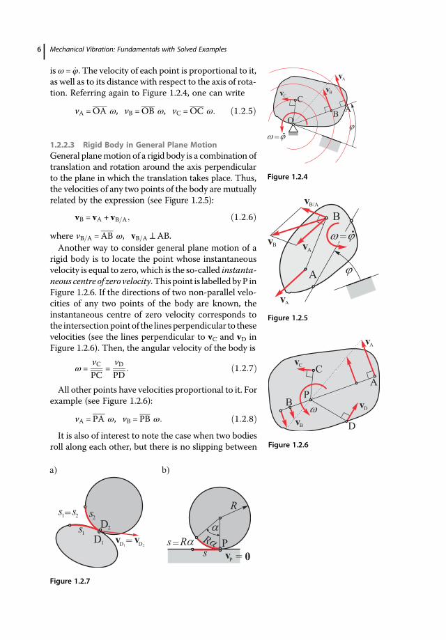
isω=φ. The velocity of each point is proportional to it,as well as to its distance with respect to the axis of rota-tion. Referring again to Figure 1.2.4, one can write

vA =OA ω, vB =OB ω, vC =OC ω 1 2 5

1.2.2.3 Rigid Body in General Plane MotionGeneral planemotion of a rigid body is a combination oftranslation and rotation around the axis perpendicularto the plane in which the translation takes place. Thus,the velocities of any two points of the body are mutuallyrelated by the expression (see Figure 1.2.5):

vB = vA + vB A 1 2 6

where vB A =AB ω, vB A ⊥AB.Another way to consider general plane motion of a

rigid body is to locate the point whose instantaneousvelocity is equal to zero, which is the so-called instanta-neous centre of zero velocity. This point is labelled byP inFigure 1.2.6. If the directions of two non-parallel velo-cities of any two points of the body are known, theinstantaneous centre of zero velocity corresponds tothe intersectionpoint of the lines perpendicular to thesevelocities (see the lines perpendicular to vC and vD inFigure 1.2.6). Then, the angular velocity of the body is

ω=vCPC

=vDPD

1 2 7

All other points have velocities proportional to it. Forexample (see Figure 1.2.6):

vA = PA ω, vB = PB ω 1 2 8

It is also of interest to note the case when two bodiesroll along each other, but there is no slipping between

Figure 1.2.5

Figure 1.2.4

Figure 1.2.6

Figure 1.2.7

Mechanical Vibration: Fundamentals with Solved Examples6

them, as shown in Figure 1.2.7a,b. Then, the equalityof the arcs s1 and s2 depicted in Figure 1.2.7a musthold and the velocities of the contact points are equal(vD1 = vD2). Analogously, for the disc rolling withoutslipping along a horizontal fixed plane shown inFigure 1.2.7b, the equality of the arc length Rα andthe distance s holds. The contact point is on thefixed plane, so its instantaneous velocity is zero andit represents the instantaneous centre of zero velocity(vP = 0).This case is shown in more detail in Figure 1.2.8.

Relating the velocity of the centre of the disc to itsangular velocity, one has

vC = PC ω= rω ω=vcr

1 2 9

The velocities of several other points are also shown.

1.2.3 Kinematics of Particles in Compound Motion

Let us consider the motion of a point M (Figure 1.2.9) relative to a rigid body that movesrelatively to a fixed coordinate system depicted by the axes x and y. The motion (trajec-tory, velocity, acceleration) of the point M with respect to the fixed coordinate systemx–y is called absolute. The motion of the point M with respect the body and the coor-dinate system ξ–η attached to the body is called relative. The motion of the body withrespect to the fixed coordinate systems is called transportation.The theorem on composition of velocities for a compound (composition/resultant)

motion states that the absolute velocity of the point is equal to the vector sum of therelative and transportation velocities of the point:

vM = vrel + vtr 1 2 10

Figure 1.2.8

Figure 1.2.9

Preliminaries 7

Note that if the body is in general plane motion, the transportation velocity is given by

vtr = vM = vA + vM A, 1 2 11

where the point M belongs to the body and it is located right below the point M.

1.3 From Kinetics

Kinetics deals with massive objects in motion – particles and rigid bodies – where theformer can be subjected to forces and the latter to forces and torques. This sub-section contains the basic relationships from Newton’s dynamics needed to form theirequations of motion. They are all based on free-body diagrams. This implies that theobject under consideration must be isolated, and the appropriate forces and torques thatexist due to mechanical contacts with surrounding bodies should be introduced asdescribed in Table 1.1.2.

1.3.1 Kinetics of Particles

Newton’s second law gives the vector relationship between the force F and the acceler-ation a of the particle of mass m:

ma=F 1 3 1

When the particle is subjected to the system of concurrent forces Fi, this equationbecomes

ma= Fi 1 3 2

This vector equation can be expressed in scalar form by using different coordinates(rectangular/Cartesian coordinates, polar coordinates, etc.). For example, in the rectan-gular coordinates (Figure 1.3.1), Equation (1.3.2) is transformed into two second-orderordinary differential equations

Figure 1.3.1

Mechanical Vibration: Fundamentals with Solved Examples8

mx = Fx 1 3 3

my = Fy 1 3 4

Their integration can give the velocity as well as the equations of motion x(t) and y(t).For the integration, the initial conditions for the particle initial position and initial veloc-ity are needed.Of interest for the discussions in this book is the form of the kinetic energy. A general

expression for the kinetic energy of the particle of mass m is:

T =12mv v =

12mv2 1 3 5

where v is the absolute velocity of the particle.

1.3.2 Kinetics of Rigid Bodies

1.3.2.1 Kinetics of Rigid Bodies in Translatory MotionFor a rigid body of mass m and centre of mass C, translating in plane (Figure 1.3.2), thescalar equations of motion in rectangular coordinates have the general form

mxC = Fx 1 3 6

myC = Fy 1 3 7

where the projections of forces stem from external forces (active and passive). The con-dition for translatory motion is

MC = 0 1 3 8

Figure 1.3.2

Preliminaries 9

A general expression for the kinetic energy of the rigid bodyin translatory motion is:

T =12mvC vC =

12mv2C 1 3 9

Due to the characteristics of translatory motion (seeSection 1.2.2.1), one can use the velocity of any other pointof the rigid body instead of vC.

1.3.2.2 Kinetics of Rigid Bodies in Fixed-Axis RotationFor a rigid body in fixed-axis rotation, the differential equa-tion of motion is related to a moment equation about the rotation axis through O(Figure 1.3.3) and has the form

JOφ = MO 1 3 10

where φ is the angle of rotation, and JO is the mass moment of inertia for the rotation axisthrough O. The positive sign of the moment corresponds to an increase in the angle ofrotation.A general expression for the kinetic energy of a rigid body in fixed-axis rotation is:

T =12JOω

2 1 3 11

The way to calculate the mass moment of inertia for different shapes of uniform bodiesis presented below.

On the mass moment of inertiaAccording to the parallel-axis theorem, the relationship between the mass moment ofinertia about the axis z through the centre of mass C and a parallel axis z1 throughanother point O (Figure 1.3.4) is given by

Jz1 = Jz +mb2 1 3 12

This can be written in a simplified form by indicating the points on the body:

JO = JC +mOC2; 1 3 13

this is the form that will mainly be used through this book. Mass moments of inertia ofsome common shapes are given in Table 1.3.1. Note that mass moment of inertia can becalculated based on the so-called radius of gyration i about a given axis. It represents theperpendicular distance from the axis to a particle of massm that gives an equivalent massmoment of inertia to the original object of the same mass. Thus, for example,JC≡ Jz =mi2C≡mi2z and JO≡ Jz1 =mi2O≡mi2z1 .

1.3.2.3 Kinetics of Rigid Bodies in General Plane MotionThe general equations of motion for a rigid body of massm ingeneral plane motion (Figure 1.3.5) involve the vector equa-tion of motion of the centre of mass C and the equation ofrotation around the axis through the centre of mass.

Figure 1.3.3

Figure 1.3.4

Mechanical Vibration: Fundamentals with Solved Examples10

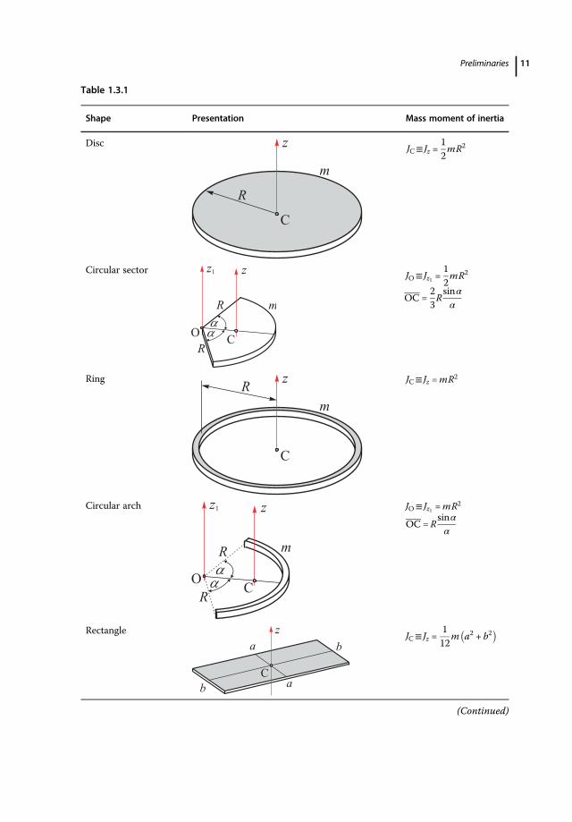
Table 1.3.1

Shape Presentation Mass moment of inertia

DiscJC≡ Jz =

12mR2

Circular sectorJO≡ Jz1 =

12mR2

OC =23Rsinαα

Ring JC≡ Jz =mR2

Circular arch JO≡ Jz1 =mR2

OC =Rsinαα

RectangleJC≡ Jz =

112

m a2 + b2

(Continued)

Preliminaries 11

Using the rectangular coordinates for the former (see Figure 1.3.5), one can write themin the form of three second-order ordinary differential equations

mxC = Fx 1 3 14

myC = Fy 1 3 15

JCφ = MC 1 3 16

Note that the mass moment of inertia corresponds to the axis through the centre ofmass as well as that the moment on the right-hand side of Equation (1.3.16) shouldbe calculated for the centre of mass. The positive sign of the moments corresponds toan increase in the angle of rotation.

Table 1.3.1 (Continued)

Shape Presentation Mass moment of inertia

EllipseJC≡ Jz =

14m a2 + b2

Slender rodJC≡ Jz =

112

ml2

Figure 1.3.5

Mechanical Vibration: Fundamentals with Solved Examples12

A general expression for the kinetic energy of the rigid body in general plane motion isgiven by the sum of two terms – one corresponding to the kinetic energy of translatorymotion and the other to rotation around the axis through the centre:

T =12mv2C +

12JCω

2 1 3 17

Alternatively, given the kinematics of this motion (see Section 1.2.2.3), the kineticenergy can also be determined based on:

T =12JPω

2 1 3 18

where P stands for the instantaneous centre of zero velocity.

1.4 From Strength of Materials

Chapter 8 of this book contains the investigations of oscillations of certain continuoussystems: longitudinal (axial) vibration of bars, torsional vibration of shafts and transver-sal vibration of beams. These investigations require the use of certain facts and expres-sions from Strength of Materials and they are presented herein for three types of loading.

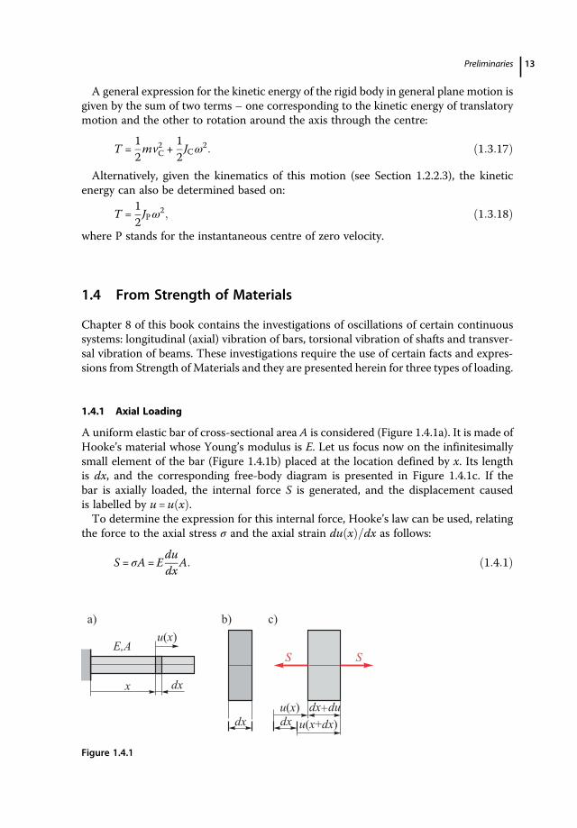
1.4.1 Axial Loading

A uniform elastic bar of cross-sectional area A is considered (Figure 1.4.1a). It is made ofHooke’s material whose Young’s modulus is E. Let us focus now on the infinitesimallysmall element of the bar (Figure 1.4.1b) placed at the location defined by x. Its lengthis dx, and the corresponding free-body diagram is presented in Figure 1.4.1c. If thebar is axially loaded, the internal force S is generated, and the displacement causedis labelled by u=u x .To determine the expression for this internal force, Hooke’s law can be used, relating

the force to the axial stress σ and the axial strain du x dx as follows:

S = σA=Edudx

A 1 4 1

Figure 1.4.1

Preliminaries 13

1.4.2 Torsion

The object of interest is a uniform elastic shaft of polar moment of inertia Io(Figure 1.4.2a). The shaft is made of a material whose shear modulus is G. The infinites-imally small element of length dx, placed at location x is considered (Figure 1.4.2b), andthe corresponding free-body diagram is presented in Figure 1.4.2c.The internal torques (twisting torques) acting on this element are labelled by M, and

the angle of rotation (twist) is labelled by φ=φ x . They are mutually related by theexpression:

M =GIodφdx

1 4 2

1.4.3 Bending

Bending of beams is considered now (Figure 1.4.3a). The uniform beam is assumed to bemade of Hooke’s material whose Young’s modulus is E. The moment of inertia of thebeam cross-section about the neutral axis is labelled by I. The displacement u of eachsection depends on its location x, that is, u=u x . An infinitesimally small element oflength dx is shown in Figure 1.4.3b. Its free-body diagram is presented inFigure 1.4.3c. This element is subjected to internal forces and bending moments M.The internal forces include shear forces Fs and axial forces, which are not shown forbrevity.

Figure 1.4.2

Figure 1.4.3

Mechanical Vibration: Fundamentals with Solved Examples14