mechanical considerations in fracture...
TRANSCRIPT

Mechanical considerations
in fracture fixation
Thesis submitted by
Pushpanjali Krishnakanth
B.E., MSc
This thesis is submitted in fulfillment of the requirements for
the degree of Doctor of Philosophy
Institute of Health and Biomedical Innovation
School of Engineering Systems
Faculty of Built Environment and Engineering
Queensland University of Technology
Brisbane, Australia
2012


Abstract
P a g e | iii
Abstract
Bone’s capacity to repair following trauma is both unique and astounding.
However, fractures sometimes fail to heal. Hence, the goal of fracture treatment is
the restoration of bone’s structure, composition and function. Fracture fixation
devices should provide a favourable mechanical and biological environment for
healing to occur.
The use of internal fixation is increasing as these devices may be applied with less
invasive techniques. Recent studies suggest however that, internal fixation devices
may be overly stiff and suppresses callus formation. The degree of mechanical
stability influences the healing outcome. This is determined by the stiffness of the
fixation device and the degree of limb loading. This project aims to characterise the
fixation stability of an internal plate fixation device and the influence of
modifications to its configuration on implant stability. As there are no standardised
methods for the determination of fixation stiffness, the first part of this project
aims to compares different methodologies and determines the most appropriate
method to characterise the stiffness of internal plate fixators.
The stiffness of a fixation device also influences the physiological loads
experienced by the healing bone. Since bone adapts to this applied load by
undergoing changes through a remodelling process, undesirable changes could
occur during the period of treatment with an implant. The second part of this
project aims to develop a methodology to quantify remodelling changes. This
quantification is expected to aid our understanding of the changes in pattern due
to implant related remodelling and on the factors driving the remodelling process.

Abstract
P a g e | iv
Knowledge gained in this project is useful to understand how the configuration of
internal fixation devices can promote timely healing and prevent undesirable bone
loss.

Keywords
P a g e | v
Keywords
Bone healing
Bone density
Bone geometry
Bone remodelling
Contra-lateral bone
Fixation stability
Internal fixation
Fixator configuration


Table of Contents
P a g e | vii
Table of Contents Abstract .............................................................................................................................................. iii
Keywords ............................................................................................................................................. v
List of figures .................................................................................................................................. xii
List of tables .................................................................................................................................. xvii
Abbreviations ............................................................................................................................. xviii
Authorship ....................................................................................................................................... xx
1.1 Background .......................................................................................................................... 2
1.2 Problem description ......................................................................................................... 2
1.3 Research question and scope ........................................................................................ 4
1.3.1 Research question ..................................................................................................... 4
1.3.2 Scope .............................................................................................................................. 4
1.4 Thesis outline ...................................................................................................................... 5
Section 1: Fixation stability and healing ....................................................................... 5
Section 2: Fixation stability and remodelling ............................................................. 6
2.1 Bone ......................................................................................................................................... 8
2.1.1 Function of a bone ..................................................................................................... 9
2.1.2 Structure, type and composition of bone ......................................................... 9
2.1.3 Bone growth and development .......................................................................... 13
2.1.4 Bone modelling and remodelling ...................................................................... 15
2.2 Bone fractures ................................................................................................................... 16
2.2.1 Fracture healing process ...................................................................................... 18
Primary fracture healing .................................................................................................. 18
Secondary fracture healing .............................................................................................. 18
2.2.2 Factors influencing fracture healing process ............................................... 20
Mechanical factors (fixation stability) and blood supply influencing fracture
healing process .......................................................................................................................... 20
2.3 Fracture treatment ...................................................................................................... 22
2.3.1 Principles of fracture fixation ......................................................................... 23
2.3.2 Types of fracture fixation devices................................................................. 27
2.4 Influence of fixation stability on healing and remodelling .......................... 30
1 Introduction ....................................................................................................................................... 1
2. Literature review.............................................................................................................................. 7

Table of Contents
P a g e | viii
2.4.1 Fixation stability and healing ......................................................................... 31
2.4.2 Fixation stability and remodelling ............................................................... 32
2.5 Finite Element Analysis (FEA) ............................................................................... 33
2.6 Computed Tomography (CT) of bones ................................................................ 34
2.7 Animal (ovine) models in orthopaedic research............................................. 35
Introduction .................................................................................................................................... 37
Problem description .................................................................................................................... 39
Goal ..................................................................................................................................................... 42
Structure .......................................................................................................................................... 42
3.1 Introduction ....................................................................................................................... 44
3.2 Materials and methods .................................................................................................. 48
3.2.1 Internal fixator ......................................................................................................... 48
3.2.2 Implant-Cylinder construct ................................................................................. 49
3.2.3 Implant-Bone construct........................................................................................ 49
3.2.4 Creation of Finite Element (FE) model ........................................................... 50
3.2.5 Boundary Conditions ............................................................................................. 51
3.2.6 Analysis ....................................................................................................................... 55
3.3 Results .................................................................................................................................. 56
3.4 Discussion ........................................................................................................................... 59
3.4.1 Method of stiffness calculation .......................................................................... 60
3.4.2 Boundary Conditions for stiffness determination ..................................... 61
3.4.3 Bone contoured geometry versus simple cylinder .................................... 64
3.5 Conclusion .......................................................................................................................... 66
4.1 Introduction ....................................................................................................................... 68
4.2 Materials and methods: ................................................................................................. 71
4.2.1 Internal fixator ......................................................................................................... 71
4.2.2 Implant-Bone analogue construct .................................................................... 71
4.2.3 Finite element model ............................................................................................. 72
4.2.4 Stiffness determination ........................................................................................ 73
4.2.5 Configurations .......................................................................................................... 74
4.3 Results .................................................................................................................................. 76
Section 1 Fixation stability and healing ................................................................................... 37
3 Development of a method to determine internal plate fixator stiffness .................. 43
4 Investigation of the influence of fixator configuration on fixation stiffness ........... 67

Table of Contents
P a g e | ix
4.3.1 Standard configuration ......................................................................................... 76
4.3.2 Internal fixator material properties ................................................................. 77
4.3.3 Internal fixator offset ............................................................................................. 77
4.3.4 Internal fixator inclination ................................................................................... 78
4.3.5 Screw configuration ............................................................................................... 79
4.3.6 Far cortical locking ................................................................................................. 80
4.4 Discussion ........................................................................................................................... 80
Introduction .................................................................................................................................... 87
Problem description..................................................................................................................... 88
Goal ..................................................................................................................................................... 90
Structure ........................................................................................................................................... 90
5.1 Introduction ....................................................................................................................... 92
5.1.1 Previous bone-remodelling quantification methods ................................. 93
5.1.2 Use of contra-lateral ovine tibia as a pre-operative control in bone
remodelling analysis ................................................................................................................ 94
Contra-lateral bone ............................................................................................................. 94
Ovine tibia .............................................................................................................................. 95
5.1.3 Goal ............................................................................................................................... 96
5.1.4 Validation of bone-remodelling algorithms .................................................. 96
5.2 Material and methods..................................................................................................... 97
5.2.1 Intact left and right tibia comparison .............................................................. 97
Geometry comparison ....................................................................................................... 99
Bone density comparison .............................................................................................. 100
5.2.2 Comparison of operated and intact contra-lateral tibia: (Empty defect
group) 104
5.3 Results ............................................................................................................................... 106
5.3.1 Intact left and right tibia comparison ........................................................... 106
Geometry comparison .................................................................................................... 106
Density comparison ......................................................................................................... 108
5.3.2 Comparison of operated and intact contra-lateral tibia: Empty defect
(3 months post-operative) ................................................................................................. 111
Section 2 Fixation stability and remodelling ........................................................................ 87
5 Development of a method to quantify remodelling changes ....................................... 91
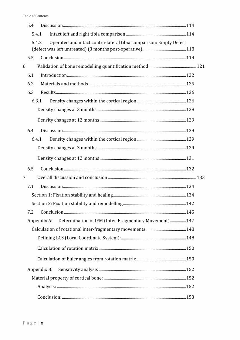
Table of Contents
P a g e | x
5.4 Discussion ......................................................................................................................... 114
5.4.1 Intact left and right tibia comparison ........................................................... 114
5.4.2 Operated and intact contra-lateral tibia comparison: Empty Defect
(defect was left untreated) (3 months post-operative) ........................................... 118
5.5 Conclusion ........................................................................................................................ 119
6.1 Introduction ..................................................................................................................... 122
6.2 Materials and methods ................................................................................................ 125
6.3 Results ................................................................................................................................ 126
6.3.1 Density changes within the cortical region ................................................ 126
Density changes at 3 months ........................................................................................ 128
Density changes at 12 months ..................................................................................... 129
6.4 Discussion ......................................................................................................................... 129
6.4.1 Density changes within the cortical region ................................................ 129
Density changes at 3 months ........................................................................................ 129
Density changes at 12 months ..................................................................................... 131
6.5 Conclusion ........................................................................................................................ 132
7.1 Discussion ......................................................................................................................... 134
Section 1: Fixation stability and healing ........................................................................ 134
Section 2: Fixation stability and remodelling .............................................................. 142
7.2 Conclusion ........................................................................................................................ 145
Appendix A: Determination of IFM (Inter-Fragmentary Movement) ................ 147
Calculation of rotational inter-fragmentary movements ........................................ 148
Defining LCS (Local Coordinate System): ................................................................ 148
Calculation of rotation matrix ...................................................................................... 150
Calculation of Euler angles from rotation matrix ................................................. 150
Appendix B: Sensitivity analysis ...................................................................................... 152
Material property of cortical bone: ................................................................................. 152
Analysis: ............................................................................................................................... 152
Conclusion: .......................................................................................................................... 153
6 Validation of bone remodelling quantification method ............................................... 121
7 Overall discussion and conclusion ....................................................................................... 133

Table of Contents
P a g e | xi
Appendix C: Comparison of Finite Element Analysis (FEA) results against
mechanical or in-vitro tests ................................................................................................... 154
FE model comparison: Cylinder-fixator model .......................................................... 154
Mechanical testing: .......................................................................................................... 155
Testing equipment in use: ............................................................................................. 155
Set up of tracking system .............................................................................................. 156
Testing .................................................................................................................................. 156
FE analysis: ......................................................................................................................... 156
Transformation of 3D model into mechanical testing coordinate system: 157
Analysis: ............................................................................................................................... 159
Conclusion:.......................................................................................................................... 160
Appendix D: Journal Paper: Can the contra-lateral limb be used as a control
with respect to analyses of bone remodelling? (Published) ..................................... 161
References ....................................................................................................................................................167

List of figures
P a g e | xii
List of figures
Figure 1 Shows the surface of a sheep tibia reconstructed from computed
tomography (CT) data using AMIRA software (Visage Imaging GmbH, Berlin,
Germany) used for illustration of the three regions of a tibia. ........................................ 10
Figure 2 Cross sectional view of a long bone.. ...................................................................... 11
Figure 3 Cross sectional view illustrating types of bone.. ................................................ 11
Figure 4 Schematic representation showing types of bone cells.. ................................ 12
Figure 5 Demonstrates skeletal development of long bone growth through
endochondral ossification.............................................................................................................. 14
Figure 6 Illustrates types of fracture lines.. ........................................................................... 17
Figure 7 Shows an X-Ray image of a fracture.. ...................................................................... 17
Figure 8 Shows schematic of a section through an intact long bone.. ......................... 19
Figure 9 Illustrates fracture healing stages: (a) inflammation phase; (b) callus
differentiation phase, (c) endochondral ossification phase and (d) Restoration of
original geometry of bone. ............................................................................................................. 19
Figure 10 Müllers plate design achieves inter-fragmentary compression by
tightening a tensioner that is temporarily anchored to the bone and the plate.. ..... 24
Figure 11 Illustrates tension band principle.. ....................................................................... 25
Figure 12 Shows an X-ray illustrating bridging osteosynthesis.. .................................. 27
Figure 13 Hoffman external fixator.. ........................................................................................ 27
Figure 14 Ilizarov external fixator.. .......................................................................................... 28
Figure 15 Plaster cast.. ................................................................................................................... 28
Figure 16 Intramedullary nail and screws.. ........................................................................... 29

List of figures
P a g e | xiii
Figure 17 Generic locking plate (modified from standard 4.5mm Locking
Compression Plate). .......................................................................................................................... 31
Figure 18 Callus histology after 6 weeks of healing.. ......................................................... 33
Figure 19 Shows the generic internal fixator attached to a cylinder. The outermost
screw holes were left empty to replicate the behaviour of a 7-hole plate with a
working of length of one empty hole spanning the fracture gap. The plate is offset
from the outer surface of cylinder by 1 mm............................................................................ 49
Figure 20 Shows the generic internal fixator attached to an ovine tibia. ................... 50
Figure 21 This close-up view of the plate-cylinder construct shows the relative
mesh densities for the components, the finest mesh was applied to the plate and
screws. The plate is offset from the outer surface of cylinder by 1 mm. ..................... 51
Figure 22 Schematic shows the MPC boundary condition. (DoFs = Degrees of
Freedom). ............................................................................................................................................. 53
Figure 23 Schematic shows the boundary conditions employed in each of the load
cases as defined by Kassi et al and Augat et al as well as the for the application of
loads via MPC. ..................................................................................................................................... 54
Figure 24 Shows the stiffness components determined for each of the three
investigated boundary conditions using implant-cylinder construct. .......................... 58
Figure 25 Shows the stiffness components determined for the internal fixator
affixed at an offset distance of 3 mm to a hollow cylinder and a bone contoured
geometry using MPC boundary condition. .............................................................................. 59
Figure 26 Shows the axial compressional stiffness value determined via stiffness
matrix method for different axial IFM’s (-0.69 mm - -0.73 mm) for the medial-
lateral bending load case. ............................................................................................................... 61
Figure 27 Internal fixator and bone cylinder construct in the standard
configuration (0xxx0xxx0) for an effective plate length of 7-hole with three screws
on either side of the osteotomy gap. .......................................................................................... 72

List of figures
P a g e | xiv
Figure 28 Illustration of calculation of axial component of IFM (Inter Fragmentary
Movement) using MPC (Multi Point Constraint) BC (Boundary Condition). ............. 74
Figure 29 Schematic representation of the screw configurations investigated.
(Notation: e.g. Top left 0XXX0XXX0, Top right X0XX0XX0X). .......................................... 75
Figure 30 Shows a generic locking plate (modified from 9 hole, 4.5 mm standard
Locking Compression Plate) with three screws on either side of the fracture gap
leaving the middle screw hole empty. ....................................................................................... 75
Figure 31 Schematic (plan/top view) represents principal of FCL in FE analysis. 76
Figure 32 Shows the division of an intact tibia into regions (proximal, diaphyseal
and distal). ......................................................................................................................................... 100
Figure 33 A colour map display of HU values across the cortex (illustrating
gradient in HU near the boundary). ......................................................................................... 102
Figure 34 The CT data was divided into four quarters (medial, lateral, anterior and
posterior) for determination of density differences. ........................................................ 104
Figure 35 shown here are transverse cross-sections of CT data of intact (figure on
left) and operated (figure on right) tibia divided into four quarters (medial, lateral,
anterior and posterior). A compression plate was affixed medially with bi-cortical
screws. ................................................................................................................................................. 105
Figure 36 (a): Shows the shell-to-shell deviation of an intact tibia pair (left and
right). Grey regions indicate a deviation of less than 1mm. The average shell-to-
shell deviation along the whole tibial length for this pair is 0.32 mm. (b): Shows the
regional (proximal, diaphyseal/shaft and distal regions) deviation. The average
shell-to-shell deviation in this case is 0.29 mm for the proximal, 0.41 mm for the
distal and 0.19 mm for the diaphyseal/shaft region. Grey regions indicate a
deviation of less than 0.5 mm. .................................................................................................... 108
Figure 37 Shows a density difference (%) histogram for intact left and right tibiae
pairs for the quarter volumes analysed (n =8). ................................................................... 109
Figure 38 Shows the density difference (left vs. right) in percentage in each of the
four (medial, lateral, anterior and posterior) quarters for a sheep tibia .................. 110

List of figures
P a g e | xv
Figure 39 Shows the bone loss, as percentage change in density in each of the four
(medial, lateral, anterior and posterior) quarters for a sheep tibia with segmental
defect (SD) treated with a compression plate 3 months after surgery. .................... 112
Figure 40 Shows the peak density difference (%) in all quarters around the screw
holes and the segmental defect (SD) between the operated and intact contra-lateral
tibia at 3 months. ............................................................................................................................ 113
Figure 41 Shows a density difference (%) histogram for intact left and right tibiae
pairs (dark grey) and operated and contra-lateral tibiae pairs (light grey) for the
quarter volumes analysed (n =8). ............................................................................................ 114
Figure 42 Shows the percentage density difference between adjacent CT slices of a
tibia in the medial quarter for one tibia pair. The lateral, anterior and posterior
quarters also showed density differences of < 2% between adjacent transverse
slices along the diaphyseal region of the tibia..................................................................... 117
Figure 43 Representative 3D CT reconstructions of critical segment bone defects,
which were left untreated (A), reconstructed with a mPCL-TCP scaffold (B) and a
mPCL-TCP scaffold combined with rhBMP-7 (C).. ............................................................. 123
Figure 44 Demonstrates the differences in load transmission path between empty
defect and groups with PCL-TCP scaffold. ............................................................................ 124
Figure 45 Shows the change in density (%) at 3 months for the medial (a) and
lateral (b) aspects of the tibia for the empty defect (Black), scaffold (Light Grey)
and scaffold with BMP (Dark Grey) groups (mean ± standard deviation).
SD=Segmental Defect. ................................................................................................................... 127
Figure 46 Shows the change in density (%) at 12 months for the medial (a) and
lateral (b) aspects of the tibia for the scaffold (Light Grey) and scaffold with BMP
(Dark Grey) groups (mean ± standard deviation). SD=Segmental Defect. ............... 128
Figure 47 Illustrates calculation of translational inter-fragmentary movements.
................................................................................................................................................................ 147

List of figures
P a g e | xvi
Figure 48 Illustration of calculation procedure for unit vectors that forms the LCS
and the Rotation Transformation Matrix (RTM). (ULCSO = Upper Local Coordinate
System at time zero). ..................................................................................................................... 149
Figure 49 shows the axial compressional stiffness value determined for the chosen
Young’s modulus (14 GPa – 24 GPa) using implant-PVC construct. ............................ 153

List of tables
P a g e | xvii
List of tables
Table 1 Lists the inter-fragmentary movements for the six load cases and the
stiffness components determined from either the stiffness matrix (Km) or the
individual stiffness (Ki) for the implant-bone construct. .................................................. 57
Table 2 The effect of implant material properties on the stability of internal plate
fixation. .................................................................................................................................................. 77
Table 3 The effect of implant offset to the bone on the stability of internal plate
fixation. .................................................................................................................................................. 77
Table 4 The effect of implant inclination to the bone on the stability of internal
plate fixation. ....................................................................................................................................... 78
Table 5 The effect of working length on the stability of internal plate fixation. ...... 79
Table 6 The effect of working length on the stability of internal plate fixation. ...... 79
Table 7 The effect of bi-cortical versus far cortical locking on the stability of
internal plate fixation. ...................................................................................................................... 80
Table 8 Contains the average distance between the outer surfaces (shell/shell
deviation) for each tibia pair (intact left and right tibia) for the whole tibia and for
the proximal, distal and diaphyseal regions separately. Additionally, the
percentage of measured points within a 1 mm tolerance is given in brackets. ..... 106
Table 9 Lists the displacement of the proximal cup determined for the axial
compressional and torsional load cases for both the FE simulation and mechanical
tests (‘X’ represents a filled screw hole and ‘0’ represents an empty screw hole).
................................................................................................................................................................ 159

Abbreviations
P a g e | xviii
Abbreviations
FEA - Finite Element Analysis
IFM - Inter-fragmentary Movement
FCL Far Cortical Locking
LCP - Locking Compression Plate
CT - Computed Tomography
AP - Anterior-Posterior
ML - Medial-Lateral
MPC - Multi Point Constraint
3D - 3 Dimensional
BC - Boundary Condition
DoFs - Degrees of Freedom
BMD - Bone Mineral Density
HU - Hounsfield Unit
EFP - European Forearm Phantom
DICOM Digital Imaging and Communications in Medicine
PVE - Partial Volume Effect
BMP - Bone Mineral Protein
SD - Segmental Defect

Abbreviations
P a g e | xix
LCS - Local Coordinate System
ULCS - Upper Local Coordinate System
LLCS - Lower Local Coordinate System
GCS - Global Coordinate System

Authorship
P a g e | xx
Authorship
I declare that the work contained in this thesis has not been previously submitted
to meet the requirements for an award at this or any other higher education
institution. To the best of my knowledge and belief, the thesis contains no
materials previously published or written by another person except where due
references is made in the text.
……………………………………..
Pushpanjali Krishnakanth Date:……………………

P a g e | 1
1 Introduction
In this introductory section, the goals of the thesis will be listed. Finally, a thesis
outline presents the structure of the thesis.

Chapter 1 Introduction
P a g e | 2
1.1 Background
Bone is a vital skeletal tissue whose primary role is to provide support for the
body, protect the internal organs and enable in locomotion. Fractures occur when
bone fails to withstand the external force exerted upon them. The self-regenerating
capability of the bony skeleton helps bone fractures to heal without any surgical
intervention. However, sometimes, they fail to heal in a timely way without
treatment. Hence the goal of any fracture treatment is to restore bone’s structure,
composition and shape by providing a favourable mechanical and biological
environment necessary for successful and timely healing.
1.2 Problem description
There are many different kinds of fixation devices available for fracture treatment.
Regardless of the choice of fixation device, fixation stability is known to have an
influence on healing outcome and the degree of stability is determined by the
stiffness of the fixator. Fixation devices used to treat fractures are broadly
classified under (i) external and (ii) internal fixators. Recent developments in both
design and surgical techniques have led to rapid adoption of internal fixation
technology. Internal fixation technique is expected to provide sufficient stability
for healing to occur whilst allowing certain amount of inter-fragmentary
movements (flexible fixation) stimulating callus formation. On the contrary, there
have been recent reports regarding the internal fixators being too rigid (Kubiak et
al., 2006; Bottlang et al., 2010; Lujan et al., 2010; Bottlang and Feist, 2011) thus
hindering fracture healing due to insufficient callus formation. There is lack of
report in terms of stiffness requirements of internal fixation devices for timely and
efficient healing. Stability of fixation is assessed by determining the stiffness of the

Chapter 1 Introduction
P a g e | 3
fixation device. Investigation of the influence of internal fixator configuration on
implant stability requires a suitable fixation stiffness determination method. Many
stiffness determination methods have been reported that differ in the manner and
orientation in which loads are applied and the manner in which displacements are
measured and stiffness calculated (Törnkvist and Hearn TC, 1996; Kassi et al.,
2001; Stoffel et al., 2003; Epari et al., 2007). In conclusion, the stiffness
requirements of these devices (internal fixation devices) are not well understood
and furthermore it is still unclear, how the configuration of the internal fixator
influences fixation stability. Additionally, there is no universal method for the
assessment of fixation stability which makes it harder to choose a particular
method in the characterisation of internal fixation devices.
Secondly, fixation stability is also known to influence the loading experienced by
the bone. Bone’s adaptation of its mass and structure to changes in its mechanical
loading through a process of remodelling is well documented. Undesirable
changes, such as bone loss, can occur due to changes in the load distribution
caused by the introduction of an implant. In the case of fracture fixation, such
reduction in mechanical competence of the bone (bone loss) can lead to implant
loosening and ultimately osteosynthesis failure. The implant chosen for fracture
treatment should prevent such undesirable bone loss leading to implant failure. In
order to understand the mechanism behind implant related bone remodelling,
quantifications of implant related changes in bone density due to remodelling is
necessary.

Chapter 1 Introduction
P a g e | 4
1.3 Research question and scope
1.3.1 Research question
In view of the above mentioned research problem, the research question which
needs to be addressed is;
Can an internal plate fixation device be configured such that
a) It promotes healing
b) Does not produce undesirable bone loss through remodelling
The specific goals of this PhD project will be firstly, (i) to develop a method to
characterise the stiffness of an internal plate fixation device. The developed
tool will then be used to investigate the influence of modifications to its
configuration on implant stability. The knowledge thus gained can be used in
future in the configuration of internal fixation devices for better healing. Secondly,
(ii) to develop a method to quantify changes due to implant related bone
remodelling. The developed method will then be used to investigate the pattern of
remodelling for different treatment groups and at different post-operative time
points. The developed remodelling quantification method can be used to validate
bone remodelling algorithms which are used to predict remodelling changes
around an implant. Then, the validated remodelling algorithms can aid in the
configuration of internal fixation devices that does not produce bone loss through
remodelling.
1.3.2 Scope
Mechanical considerations in fracture fixation include investigation of the
influence of fixation stability on; healing, implant related changes due to bone

Chapter 1 Introduction
P a g e | 5
remodelling and implant survival. This project investigates the influence of
fixation stability on healing and remodelling.
1.4 Thesis outline
This thesis investigates the importance of fixation stability on both healing and
implant induced bone remodelling. The chart below shows how these two
elements, discussed in two sections are linked together in this thesis.
Section 1: Fixation stability and healing
The prime aim of this section of the project is to understand how fixator
configuration (internal plate fixator) influences stiffness. In accomplishing this,
there are several sub aims, which will be addressed in Chapters 3 and 4
individually.
Chapter 1: Project Goals
Chapter 2: Literature Review
Section 1
Fixation stability and healing
Chapter 3
Chapter 4
Section 2
Fixation stability and remodelling
Chapter 5
Chapter 6
Chapter 7: Overall discussion and conclusion

Chapter 1 Introduction
P a g e | 6
Chapter 3: Development of a method to determine internal plate fixator
stiffness
Chapter 4: Investigation of the influence of fixator configuration on fixation
stiffness
Section 2: Fixation stability and remodelling
After having investigated the influence of fixator configuration on implant stability,
the next task is to investigate the influence of the fixator stiffness on implant
related remodelling changes. In doing so, firstly, the mechanisms that regulate
implant related bone-remodelling process has to be understood. Hence,
quantification of bone-remodelling in experimental situations is necessary and
is realised in Chapter 5 of this PhD thesis.
Chapter 5: Development of a method to quantify changes due to remodelling
Chapter 6: Further validation of the bone remodelling quantification method
Chapter 7: Overall discussion and conclusion
P a g e | 7
2. Literature review
This chapter provides a review of relevant literature. This chapter begins with an
introduction to basic anatomy of bone, including its functional adaptation. This is
then followed by a description of fractures, fracture healing mechanisms,
mechanical factors influencing the healing process along with an introduction of
fracture fixation devices. Finally discussion of the influence of fixator configuration
on its stiffness and in turn its influence on bone-remodelling concludes the
chapter.

Chapter 2 Literature review
P a g e | 8
2.1 Bone
Bone is a highly complex skeletal tissue accounting for approximately 14% of body
weight in an average person (Steele, 1990). The adult skeleton consists of 206
distinct bones divided as follows (Gray, 1918).
Axial skeleton
o Vertebral column – 26
o Skull – 22
o Hyoid bone – 1
o Ribs and sternum – 25
Appendicular skeleton
o Upper extremities – 64
o Lower extremities – 62
o Auditory ossicles – 6
The above mentioned 206 bones fall in any one of the four broad classes (Bartel,
2006).
Long bones, which are long in one direction with tubular cross sections in the
central shaft (diaphysis), such as femur, the tibia, and the humerus.
Short bones, which are bones or portions of bones, which have same
dimensions in all directions, such as bones of the wrist and ankle.
Flat bones or tabular bones, which are smaller in one dimension than in the
others, and make up portions of skull, the scapula, the pelvis and the transverse
processes of vertebrae.
Irregular bones are the ones which do not fall in any of the above three
categories, such as vertebral bodies and the posterior elements.

Chapter 2 Literature review
P a g e | 9
2.1.1 Function of a bone
Bone’s primary role is to provide support for the body and help in locomotion by
providing a strong supportive and mechanically optimal structure for the soft
tissues and muscles (Webb and Tricker, 2000; Bartel, 2006). Bone’s surfaces are
the attachment sites and lever arms for muscles, tendons and ligaments that aid in
posture and move the body parts (Steele, 1990).
In order to perform its primary role, bone should be stiff and strong as well as light
in weight. The strength and stiffness of a bone is determined by the architecture
(shape and dimensions) and mechanical quality of the bone material. Strength and
stiffness of the bone change with bone mass and structure, with noticeable changes
during its growth, remains in more or less constant in adulthood and deteriorates
in the elder. The mechanical loading environment is known to have an influence on
bone’s mass and structure (Mow, 2005). Hence bone is an adaptive tissue.
2.1.2 Structure, type and composition of bone
As shown in Figure 1, long bones, are divided into three identifiable regions
namely; Epiphysis, metaphysis and diaphysis. The cortex forms a tube surrounding
a hollow medullary cavity. Spongy or cancellous bone is found towards the ends of
the bones and near the internal cortex surface. From inside as well as outside,
bones are surrounded by connective tissue and membranes; Periosteum covers the
bone externally. While cartilage covers the articular surfaces and the internal
marrow cavities are lined by endosteum. Both endosteum and periosteum contain
bone manufacturing cells. Red marrow which forms blood cells exists within the
medullary cavity and inter-trabecular spaces in the cancellous bone (Steele, 1990).
Chapter 2 Literature review
P a g e | 10
Figure 1 Shows the surface of a sheep tibia reconstructed from computed
tomography (CT) data using AMIRA software (Visage Imaging GmbH, Berlin,
Germany) used for illustration of the three regions of a tibia.
Primarily, there are three types of bone:
Woven bone (not illustrated in Figure 2) formed during embryonic development
or during fracture healing (callus) (Fredric, 2002) is composed of randomly
arranged collagen bundles and irregularly shaped vascular spaces lined with
osteoblasts. Woven bone is eventually replaced with cortical or cancellous bone
(Kalfas, 2001). Woven bone, due to its loose structure is mechanically inferior to
cortical bone (Currey, 2003).
Cortical or compact bone whose primary structural unit is an osteon is remodelled
from woven bone by means of vascular channels that invade the embryonic bone
from its periosteal and endosteal surfaces. Its mechanical strength depends on
how well osteons are tightly packed (Kalfas, 2001). Cortical bone comprises the
diaphysis of long bones and the thin shells that surround the metaphysis.
Proximal epiphysis
Metaphysis
Diaphysis
Distal epiphysis

Chapter 2 Literature review
P a g e | 11
Figure 2 Cross sectional view of a long bone (modified from1).
Figure 3 Cross sectional view illustrating types of bone (modified from2).
1 http://www.web-books.com/eLibrary/Medicine/Physiology/Skeletal/Skeletal.html (accessed on 12/09/2011) 2 http://www.iofbonehealth.org/health-professionals/about-osteoporosis/basic-bone-biology.html (accessed on 12/05/2009

Chapter 2 Literature review
P a g e | 12
Cancellous or trabecular bone is less dense than cortical bone (Figure 3). The
classification of bone tissue as cortical or trabecular is based on relative density.
Trabecular bone in the metaphysis and epiphysis is continuous within the inner
surface of the metaphyseal shell and exists as a three-dimensional interconnected
network of trabecular rods and plates (Mow, 2005).
Bone is comprised of three distinctly different cell types as shown in Figure 4,
namely;
Osteoblasts or bone forming cells: Osteoblasts are the cells that lay down the
extracellular matrix and regulate its mineralization (Sommerfeldt and Rubin,
2001). They secrete osteoid; un-mineralised organic matrix which subsequently
undergoes mineralization, giving the bone its strength and rigidity. Some
osteoblasts are converted to osteocytes nearing the completion of their bone
forming activity, while others remain as lining cells on the periosteal or endosteal
surfaces of bone. Osteoblasts also play a role in activating bone resorption by
osteoclasts.
Figure 4 Schematic representation showing types of bone cells (reproduced from3).
Osteocytes or bone maintaining cells: These are mature osteoblasts trapped within
the bone matrix which are involved in the control of extracellular concentration of
3 http://www.iofbonehealth.org/health-professionals/about-osteoporosis/basic-bone-biology.html (accessed on 12/09/2011)

Chapter 2 Literature review
P a g e | 13
calcium and phosphorous. They are also involved in adaptive remodelling
behaviour via cell-to-cell interactions in response to local environment.
Osteoclasts or bone-resorbing cells: These cells are multinucleated bone resorbing
cells which function in groups termed “cutting cones” that attach to bare bone
surfaces, release hydrolytic enzymes, dissolves the inorganic and organic matrices
of bone and calcified cartilage (Kalfas, 2001).
2.1.3 Bone growth and development
Bone growth occurs by two different mechanisms; while bones of skull and some
irregular bones are formed through intramembranous ossification where sheet-like
connective tissue membranes are replaced with bony tissue; most bones are
formed through endochondral ossification where hyaline cartilage is replaced by
bony tissue (National Cancer Institute, 2011). Bone resorption by osteoclasts
followed by new bone deposition by osteoblasts is a continuous process which
occurs during growth and throughout life. Bone formed by this process is called
secondary bone. Primary bone or first bone is formed through endochondral
ossification-mineralization of cartilage (as illustrated in Figure 5) or direct sub-
periosteal deposition. Around the diaphysis, osteoblasts form a collar of compact
bone. Simultaneously, cartilage at the centre of diaphysis begins to disintegrate.
Osteoblasts penetrate the disintegrating cartilage and replaces it with spongy or
trabecular bone forming primary ossification centre. Further ossification continues
extending from the ossification centre towards the bone ends. Later osteoclasts
break down the newly formed spongy bone in the diaphysis to open up a
medullary cavity. Due to the continuous growth of cartilage in epiphysis,
developing bone increases in length. After birth, ossification continues with the
formation of secondary ossification centres formed in the epiphysis. Ossification in

Chapter 2 Literature review
P a g e | 14
epiphysis differs from diaphysis ossification only by retaining spongy bone instead
of being broken down to form a medullary cavity. Hyaline cartilage is totally
replaced by bone at the completion of secondary ossification except over the
epiphysis surface where it remains as articular cartilage and as an epiphyseal plate
between epiphysis and diaphysis. The cartilage continues to grow in regions of
epiphyseal plate and next to the diaphysis. Chondrocytes next to the diaphysis age
and degenerate. Osteoblasts move in and ossify the matrix to form bone and
become trapped in the matrix as osteocytes. Other osteoblasts close off the bone
surface as lining cells (Mow, 2005). Until cartilage growth slows down and finally
stops, this process of bone growth continues throughout childhood and adolescent
years.
Figure 5 Demonstrates skeletal development of long bone growth through
endochondral ossification (modified from4).
With the increase in bone’s length with the individual’s age, the bone must increase
its diameter. This occurs through intramembranous ossification that does not
involve prior cartilage formation. The increase in diameter is called appositional 4 http://learnsomescience.com/anatomy/microscopic-structure-of-the-skeletal-system-what-makes-our-bones-strong/ (accessed on 12/09/2011)

Chapter 2 Literature review
P a g e | 15
growth. Osteoblasts in the periosteum form compact bone around the external
bone surface. At the same time, osteoclasts in the endosteum break down bone on
the internal bone surface, around the medullary cavity. These two processes
together increase the diameter of the bone while preventing bone from becoming
too bulky (National Cancer Institute, 2011).
2.1.4 Bone modelling and remodelling
Bone modelling can be defined as a process whereby bone is laid down onto
surfaces without necessarily being preceded by resorption. After ossification, bone
differentiation continues within the tissue (Mow, 2005). According to Frost
(Goodfellow and O’Connor, 1978), modelling is defined as growth and
development of the cortical and trabecular structure and later morphological
adaptation as it occurs in growth or reactions to reduced and increased external
loads.
Bone remodelling is the ongoing process of replacement of old bone by new bone.
During the remodelling process, bone is formed in places where it is needed and
removed from places where it is no longer needed .Hence it is related to removal
or maintenance of bone matrix and expressed by bone-resorbing osteoclasts and
bone forming osteoblasts, collectively known as “Basic multicellular units” or
BMU’s. Bone remodelling starts with the appearance of osteoclasts at the quiescent
bone surface which attach to the bone tissue matrix and form a ruffled border at
the bone /osteoclast interface that is completely surrounded by a “sealing zone”,
thus forming an isolated micro-environment, Osteoclasts acidify this
microenvironment and dissolve the organic and inorganic compounds of bone.
After this bone resorption stops, osteoblasts derived from mesenchymal stem cells,
periosteum and soft tissues appear at the same surface site, deposit osteoid, thus

Chapter 2 Literature review
P a g e | 16
mineralizing it to form new bone. Some osteoblasts get encapsulated in this
osteoid matrix, further differentiating to osteocytes. While others continue to
synthesize bone until they transform to form quiescent lining cells covering newly
formed bone surface. Since osteoblasts and osteoclasts together are responsible
for the remodelling process, it is believed that there exist a coupling mechanism
between formation and resorption. In cortical bone a BMU forms a cylindrical
canal. In its tip on the order of ten osteoclasts dig a circular tunnel (cutting cone)
which are followed by several thousands of osteoblasts that fill the tunnel (closing
cone), thus producing a secondary osteon of renewed bone. The remodelling
process in the trabecular bone is believed to be a surface event (Mow, 2005).
2.2 Bone fractures
Bone fractures occur when bone fails to withstand the external force exerted upon
them. Hence fractures occur as a consequence of mechanical overload whose
configuration is influenced by the material properties of the bone, the type and
magnitude of force and loading rate (Schatzker and Houlton, 1999). Bone fractures
represent a structural failure of the primary load-carrying apparatus of the body.
The uniquely biological aspect of a skeletal structure is its capability to repair
itself; bone fractures can heal without any external intervention. On the other hand
they sometimes fail to heal successfully in a timely way, without treatment. The
primary purpose of fracture treatment devices is to provide the initial structural
reinforcement and a favourable mechanical and biological environment that is
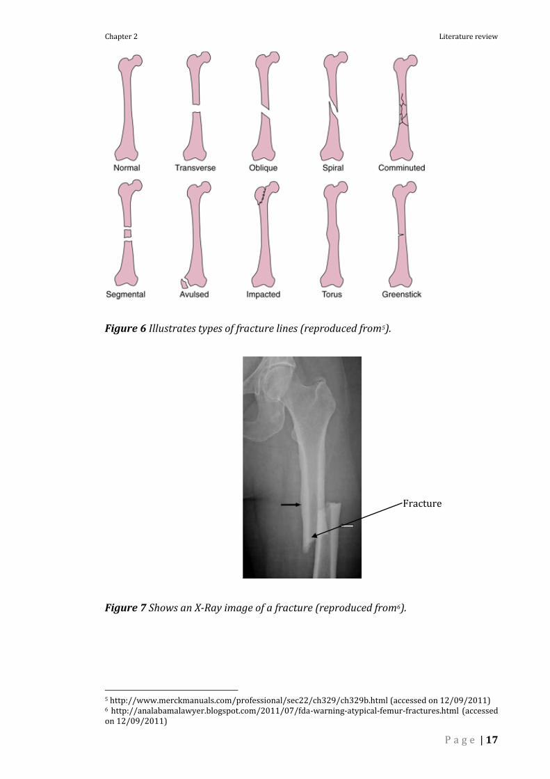
necessary for the healing to occur as quickly and uneventfully as possible (Bartel,
2006). Figure 6 illustrates different kinds of fractures and Figure 7 shows a
fracture line as seen in an X ray.
Chapter 2 Literature review
P a g e | 17
Figure 6 Illustrates types of fracture lines (reproduced from5).
Figure 7 Shows an X-Ray image of a fracture (reproduced from6).
5 http://www.merckmanuals.com/professional/sec22/ch329/ch329b.html (accessed on 12/09/2011) 6 http://analabamalawyer.blogspot.com/2011/07/fda-warning-atypical-femur-fractures.html (accessed on 12/09/2011)
Fracture

Chapter 2 Literature review
P a g e | 18
2.2.1 Fracture healing process
A fracture results in a series of tissue responses that are designed to remove tissue
debris, re-establish the vascular supply, and produce new skeletal matrices
(Simmons, 1985).
Fracture healing is divided into; a) Primary fracture healing and b) secondary
fracture healing.
Primary fracture healing
Primary fracture healing or direct bone healing requires anatomical reduction,
stabilization and compression of fracture which is seen in cases of negligible gap
size and extreme stability (Webb and Tricker, 2000; Bailón-Plaza and van der
Meulen, 2001). According to the AO group, this situation is often seen only after
open reduction and rigid internal fixation. Here, fracture tissue appears at the
fracture site, bridges the fracture site by direct Haversian remodelling (Brighton,
1985) or direct cortical modelling by the formation of cutting cones. The
osteoclasts lead the way by tunnelling across the fracture. Thus the new blood
vessels along with osteoblasts directly model the cortical bone into a Haversian
structure (Webb and Tricker, 2000). Bone on one side of the cortex unites with
bone on the other side thus re-establishing mechanical continuity (Einhorn, 1998).
Secondary fracture healing
The majority of bone fractures undergo secondary fracture healing, which requires
some motion at the fracture site. This can be achieved either by non-operative
treatment or with the aid of a surgical procedure which allows some mobility at
the fracture site (Webb and Tricker, 2000). Secondary fracture healing involves a
combination of intramembranous and endochondral ossification process which
participates in fracture healing at different stages of healing. These stages of

Chapter 2 Literature review
P a g e | 19
healing (as shown in Figure 9) is comprised of an initial stage of hematoma
formation leading to the occurrence of inflammation, a subsequent stage of
angiogenesis development and cartilage formation, further leading to three
successive stages of cartilage calcification, cartilage removal and bone formation
and ultimately leading to bone remodelling (Einhorn, 1998).
Figure 8 Shows schematic of a section through an intact long bone-(reproduced
from7).
Figure 9 Illustrates fracture healing stages: (a) inflammation phase; (b) callus
differentiation phase, (c) endochondral ossification phase and (d) Restoration of
original geometry of bone (reproduced from 8).
7 (Goodfellow and O’Connor, 1978) 8 (Goodfellow and O’Connor, 1978)

Chapter 2 Literature review
P a g e | 20
2.2.2 Factors influencing fracture healing process
The factors that influence fracture healing can be broadly divided into two
categories;
Systemic factors: Age, hormones (Cruess and Dumont, 1975), nutritional status of
patients (Webb and Tricker, 2000), Pharmacological factors like smoking,
pregnancy, diabetes and etc., are some of the systemic factors which influences
fracture healing.
Local factors: Local factors influencing fracture healing are; degree of local trauma
experienced by bone and surrounding tissue, the amount of bone loss, the type of
bone affected, degree of immobilization, state of local blood supply to the fracture
area, degree of vascularity, bioelectric factors, mechanical factors governed by the
type of fracture treatment and fixation device used, and local pathological
conditions (infection, radiation, chemical burns) (Cruess and Dumont, 1975;
Brighton, 1985).
In clinical practice it is believed that local factors affecting fracture healing are far
more important than systemic factors in most of the patients (Brighton, 1985).
Mechanical factors (fixation stability) and blood supply influencing
fracture healing process
Fracture healing has two major prerequisites; mechanical stability and sufficient
blood supply among the local factors. Influence of mechanical environment with
reference to fracture healing depends on the type of fracture fixation device used
to treat a particular fracture among other factors. The degree of mechanical
stability of a bony fracture is determined by the stiffness of a fracture fixation
device (White et al., 1977; Goodship and Kenwright, 1985; Goodship et al., 1993;

Chapter 2 Literature review
P a g e | 21
Probst et al., 1999) and is expressed in terms of inter-fragmentary strain or inter-
fragmentary movement at the fracture site. Since blood supply is equally necessary
for the nutrition of healing zone, an insufficient blood supply can cause a delayed
union or even atrophic non union (Mow, 2005). Apart from other factors
responsible for diminished blood supply, a different pattern of vascularisation can
be seen under stable and unstable fixation. However even a well vascularised
fracture healing zone will lead to a hyper-trophic non-union if the mechanical
stability is insufficient (Claes et al., 2002). Hence, both inter-fragmentary
movement or inter-fragmentary strain and amount of blood supply are equally
important for successful and uneventful healing. Few previous studies have
investigated the relationship between the degree of instability (expressed as IFM
or IFS) and amount of blood supply found in various tissues in relation to fracture
healing.
Dahlkvist et al.(1982) speculated constant rupture of capillaries required for
osseous repair, resulting in the development of fibro cartilaginous tissue, thus
delaying fracture healing under unstable fixation (Dahlkvist et al., 1982).
Bell et al (1998) quantified correlation between vascularisation and tissue
formation under well defined biomechanical conditions(Bell et al., 1998). This
study showed that greater inter-fragmentary movements in a 2-mm osteotomy gap
of the sheep metatarsal led to significantly more fibro cartilage, less bone
formation, large hydrostatic pressures which may cause blood vessels to collapse
(Mow, 2005) and a small number of vessels close to the periosteum than under
small inter-fragmentary movements.
Among the mechanical factors, fracture gap size is another factor which influences
healing (Claes et al., 1998). Claes et al (1997) showed how small gap sizes promote

Chapter 2 Literature review
P a g e | 22
fracture healing in a fast and successful manner while large gap sizes impede
fracture healing process (Claes et al., 1997).Therefore, inter-fragmentary
movement and fracture gap size seem to be the two important mechanical factors
which influence the fracture healing process. Furthermore, the sensitivity of bone
healing to initial mechanical conditions has been shown both biomechanically and
histologically (Klein et al., 2003). Since the initial mechanical environment may
have lasting implications on the course of fracture healing, a detailed
understanding of the influence of fixation stability on the mechanical conditions
within the callus is believed to improve fracture treatment.
2.3 Fracture treatment
The goal of fracture treatment is the restoration of bone’s structure, composition
and function (Bartel, 2006). Fracture treatment is mainly to achieve an anatomical
alignment of broken bone fragments, to relive pain as well as stabilize the
fragments in order to initiate bony union (Mow, 2005). Unlike other tissues, bone
has a uniquely distinct property which helps it to regenerate itself by restoring the
properties of pre-existing tissue. Most fractures are either left untreated or are
treated with a form of surgical management that results in some degree of motion
(sling immobilization, cast immobilisation, external fixation, intramedullary
fixation) (Einhorn, 1998). For fractures which are inherently stable, little
additional effort is needed to maintain a minimal amount of IFM (Inter-
Fragmentary Movement). In such cases, cast or braces is sufficient to treat such
fractures where fractures heal by secondary fracture healing involving
intramembraneous and endochondral ossification. Until twentieth century,
fracture treatment was performed by external splinting. Today, even though
majority of fractures are treated with plaster casts or braces, complex fractures,

Chapter 2 Literature review
P a g e | 23
fractures with extensive soft tissue damage; open as well as infected fractures
cannot always be treated successfully with plaster cast stabilization. Hence, the
operative treatment of fractures with new fixation systems and implants came into
existence (Mow, 2005).
From a biomechanical point of view, fracture fixation must possess sufficient
stability, which means it has to reduce inter-fragmentary movement occurring due
to external loading and muscle activity to such an extent that it promotes timely
and successful fracture healing.
2.3.1 Principles of fracture fixation
Primarily there are two main principles of fracture fixation and all the fixation
devices used to treat fractures uses any one of these two principles;
Inter-fragmentary compression stabilisation:
Under absolutely stable conditions, bone heals by a process of direct bone healing
with no or minimal callus formation (Schatzker and Houlton, 1999). This absolute
stability can be achieved when compression over the whole cross section of a
fracture is sufficiently high such that all forces and moments acting at the fracture
site are neutralised. Under such conditions, there exists no inter-fragmentary
movement between the two fracture fragments (Mow, 2005). Such an inter-
fragmentary compression can be achieved by lag screws, compression plates, and
tension band systems (Delp et al., 1990).
o Compression plate
First the fixation plate is fixed with screws on one of the bone fragments. Then
a tension device placed on the second fragment which moves the plate axially,
is used temporarily to pull both the fragments together, thus creating an inter-

Chapter 2 Literature review
P a g e | 24
fragmentary compression (Figure 10). Later the second fragment is fixed to the
plate with additional screws. Compression between two fragments can also be
achieved with plates having a tapered screw hole upon which the screw head
slides (Delp et al., 1990).When the screw is inserted into the bone, it moves
towards the bone cortex, since the slope of the screw hole is pushed axially. The
compression achieved with the help of compression plates does not change
with changing loads and muscle activity and hence static in nature (static
compression) (Mow, 2005).
Figure 10 Müllers plate design achieves inter-fragmentary compression by
tightening a tensioner that is temporarily anchored to the bone and the plate
(reproduced from 9).
o Inter-fragmentary compression by tension band principle
Bones are not always loaded by axial force alone. According to Pauwels
(Pauwels, 1958) observation, certain long bones are eccentrically loaded
which results in bending. Pauwels postulated that apart from gravity and
muscle activity, the net loading on such bones, would create a compressive
9 (Uhthoff et al., 2006)

Chapter 2 Literature review
P a g e | 25
force on side closer to loading and a tensile force on the opposite side.
Compressive forces due to body weight, bending and pure axial forces
results in inter-fragmentary compression without the need for an additional
fixator. However the tensile force created due to bending has to be
neutralized to order to prevent dislocation of fragments. This neutralisation
can be achieved by placing the implant on the tension side of the bone
(Figure 11) which is commonly known as tension band principle (Schatzker
and Houlton, 1999). Compression thus achieved change dynamically,
depending on external loads and muscle activity (Mow, 2005).
Figure 11 Illustrates tension band principle (modified from 10).
Non compressive stabilisation
As the name suggests, the fracture fragments are not pulled against each other
with any external application of compressive force. Stabilization of fragments is
obtained by attaching an implant which holds the two fragments together with the
help of screws. The healing of a bony fracture follows the course of secondary
10 (Rüedi, 2007)

Chapter 2 Literature review
P a g e | 26
healing. Fracture healing under inter-fragmentary movement occurs by callus
formation that mechanically unites the bony fragments (Mow, 2005)
o Bridging osteosynthesis with bridging plates
The fundamental principle is to leave the fracture fragments undisturbed as
shown in Figure 12. This technique relies upon the soft tissue envelope to
reconstruct an approximate cylinder of bone fragments, while the major,
proximal and distal fragments are distracted and pulled out to length. Hence
the fracture fragments are neither immobilized nor realigned; thereby leaving
tenuous soft tissue attachments left undisturbed. Bridging osteosynthesis can
be achieved by a number of techniques. A conventional plate can be used to
bridge two fracture fragments with three of four screws anchored proximally
and distally in the intact parts of the fractured bone. Two advantages have been
identified with this technique;
Since the plate extends to a sufficient length along the fracture zone,
the load on the underside of the plate not fixed to the bone can be
distributed over an extended distance thus reducing sudden increase
in stress which could lead to fatigue failure in certain areas.
As the plate is applied at a distance to the bone, it permits better
vascular supply (Schatzker and Houlton, 1999).

Chapter 2 Literature review
P a g e | 27
Figure 12 Shows an X-ray illustrating bridging osteosynthesis (modified from11).
2.3.2 Types of fracture fixation devices
There is a wide range of fracture fixation devices (as shown in, Figure 13-Figure
16) available to treat fractures which could be broadly divided under two main
categories depending on whether the device is positioned entirely inside the skin
(Internal fixator) or is partially inside the skin for bracing purposes only while the
major part of fixator remains outside the skin surface (External fixators).
External fixator: Plaster Cast and Brace; for inherently stable fractures to enhance
natural healing, unilateral frames, bilateral frames, triangular frames.
Internal fixator: Intramedullary rod or nail (reamed nail and un-reamed nail),
screws (angle stable screws and lag screws), internal fixation plates (Locking
plates with angle stable screws).
Figure 13 Hoffman external fixator (reproduced from12).
11 (Rüedi, 2007) 12 http://www.rch.org.au/limbrecon/prof.cfm?doc_id=4873 (accessed on 12/09/2011)

Chapter 2 Literature review
P a g e | 28
Figure 14 Ilizarov external fixator (reproduced from13).
Figure 15 Plaster cast (reproduced from14).
13 http://teamofmonkeys.com/html/leg.html (accessed on 12/09/2011) 14http://www.theinjurylawyers.co.uk/injury-lawyers-blog/2009/10/14/plaster-of-paris-burns-teenager/ (accessed on 12/09/2011)
Chapter 2 Literature review
P a g e | 29
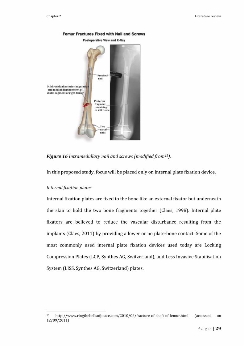
Figure 16 Intramedullary nail and screws (modified from15).
In this proposed study, focus will be placed only on internal plate fixation device.
Internal fixation plates
Internal fixation plates are fixed to the bone like an external fixator but underneath
the skin to hold the two bone fragments together (Claes, 1998). Internal plate
fixators are believed to reduce the vascular disturbance resulting from the
implants (Claes, 2011) by providing a lower or no plate-bone contact. Some of the
most commonly used internal plate fixation devices used today are Locking
Compression Plates (LCP, Synthes AG, Switzerland), and Less Invasive Stabilisation
System (LISS, Synthes AG, Switzerland) plates.
15 http://www.ringthebellsofpeace.com/2010/02/fracture-of-shaft-of-femur.html (accessed on 12/09/2011)

Chapter 2 Literature review
P a g e | 30
2.4 Influence of fixation stability on healing and remodelling
Fixation devices are used to treat fractures in order to stabilise the fracture
fragments until it heals. The mechanical stability of the bony fracture is known to
influence the healing outcome. This stability is determined by the stiffness of the
fixation device. Hence, fixation stiffness is known to influence healing. For
fractures which follow the course of secondary healing, mechanical stability is
known to be crucial for healing. Furthermore, the progressive maturation of the
fracture callus from woven to lamellar bone is known to be dependent on this
stability (Giannoudis et al., 2007). Surgical interventions such as the application of
systems of internal or external stabilisation are designed to improve stability of
fixation and thereby enhance healing. Additionally, the stiffness of the fixation
device determines the physiological loading environment of the affected limb.
Since bone is known to adapt its shape and structure to changes in loading
condition placed on it, through the remodelling process (Wolff et al., 1986),
fixation stiffness also influences remodelling.
The use of external fixators has certain disadvantages such as, the pin sites where
the metal work enters the skin and goes into the bone can sometimes be a source
of infection, the pins and rods extruding outside the skin demands extra care from
the wearer and wearing external fixators can sometimes become a social issue
with stares on street. These disadvantages can be overcome to an extent by the use
of internal fixation devices where the fixators are placed under the skin and
muscle. Also, internal fixators have gained popularity over the recent years as they
can be applied with less invasive surgical techniques. However there is still lack of
report with reference to stiffness requirements of these devices for better healing
outcome as well as restoration of bone’s structure and composition in terms of

Chapter 2 Literature review
P a g e | 31
remodelling. Therefore, this project focuses on internal plate fixators. A generic
locking plate representing a standard 9 hole 4.5 mm osteosynthesis plate and
screws commercially available from implant manufacturers was used in the
analysis (Figure 17).
Figure 17 Generic locking plate (modified from standard 4.5mm Locking
Compression Plate).
2.4.1 Fixation stability and healing
Minimal surgical technique while preserving fracture vascularity has led to rapid
adoption of internal fixation technology over the recent years. Locked internal
plates are aimed to provide elastic fixation that allows sufficient inter-fragmentary
movements (IFM) such that healing occurs via secondary bone healing with
external callus formation. This callus is then replaced by bone thus restoring the
mechanical strength and structure of the bone. The callus thus formed is known to
influence healing by providing the provisional stability (through its mass) and
strength (through its geometry) to ensure healing may progress (LaStayo et al.,
2003). The mechanical environment within the healing callus is determined by the
inter-fragmentary movements which in turn are a function of fixation stability and
limb loading. These IFM’s can be broken down into three translational and three
rotational components. However, the IFM’s during the initial healing phase have
been shown to be mainly composed of shear and axial movements (Schell et al.,
2005). While moderate axial movements are shown to be stimulatory to healing
(Claes et al., 1997), excessive shear movements are known to be detrimental to
healing (Yamagishi and Yoshimura, 1955).

Chapter 2 Literature review
P a g e | 32
These IFM’s vary inversely with fixation stability (more stable the fixator, less
IFM’s occur leading to less callus formation). The difference between beneficial
motion in the fracture gap which induces callus formation and too much motion
which leads to non-union is fairly bleak (Brennwald, 1996) Hence, it is difficult to
find the right balance between reducing the risk of plate failure (very flexible plate
leading to too much IFM) and providing optimal IFM (sufficiently flexible plate
with right amounts of IFM) to stimulate callus formation for successful healing.
Therefore, it is challenging to configure fixation devices of sufficient stability that
promotes better healing outcome.
2.4.2 Fixation stability and remodelling
The goal of fracture healing is the restoration of the mechanical properties such as
strength and stiffness of the fractured bone. Fixation devices which provide
sufficient stability to the bony fragments until it heals are chosen to treat fractures.
It is known that the load distribution on the affected limb in the presence of an
implant is determined by the stability of the fixation device used to treat fractures.
Regulation of load induced bone remodelling is well documented (Wolff et al.,
1986; Mori and Burr, 1993). Since bone adapts to changes in external loading by
undergoing changes in its shape and structure through remodelling process,
implant stability is believed to in turn influence remodelling changes.
Complications with fracture healing have been reported due to re-fractures
following stress protection by plates (Allgöwer et al., 1969). Stress protection is a
reduction in the mechanical competence of the bone in the presence of a fixator.
Figure 18 shows bone loss around an implant. By definition stress protection is a
way the implant protects the healing bone against loads that it may be temporarily
unable to sustain. Such unloading of the bone in the presence of a fixator is a result

Chapter 2 Literature review
P a g e | 33
of bone stresses being transmitted through the plate and not through the bone.
This unloading leads to bone atrophy since bone adapts to changes in its
mechanical loading and subsequently poses the threat of re-fracture after implant
removal. Hence the osteosynthesis device used to treat fractures should not only
provide sufficient stability for successful and timely healing but also should not be
too stiff to induce stress protection.
Figure 18 Callus histology after 6 weeks of healing (reproduced from16).
2.5 Finite Element Analysis (FEA)
FEA is a numerical tool used to solve complex engineering problems. When faced
with the task of solving complex engineering problems, it is often useful to
represent this complex system in terms of a simplified system or model of a system
by extracting the essential elements. This model can then be used to observe the
behaviour of the system to its response to altered input parameters or conditions.
Such modelling can be either physical modelling where real constructions are built
or mathematical modelling which uses conceptual representations. Finite element
16 (Epari, 2006)
Position of screw hole
Remodelling (bone loss) in regions adjacent to screw hole

Chapter 2 Literature review
P a g e | 34
models are numerical (rely on computers to find approximate solutions)
mathematical models (Prendergast, 1997). A system can be built by the addition of
structurally and mathematically defined finite elements, joined together by
commonly shared nodes. When the overall system is subjected to load, the
localised response of each element is calculated to form a solution to the system
load state, identifying the cause and effect relationship between loads placed on a
system and the resulting mechanical behaviour including stresses and strains. By
using this technique in an orthopaedic setting the actual mechanical environment
induced in a bone by application of a fixator can be measured and understood. FE
technique is used in orthopaedic research in many areas such as, analysis and
design of orthopaedic devices, analysis of tissue growth, remodelling and
degeneration and analysis of the skeleton. The first application of FEA in
orthopaedics was in 1972 (Brekelmans et al., 1972). Thereafter, its use in
orthopaedic research is increased with techniques and complexities increasing
rapidly in recent years. One of the prime advantages of using FE would be that it
overcomes the variability and repeatability issues encountered in
experimentation. However, any model is an attempt made to represent reality.
During such a representation, not all variables governing the process can be
considered and thus a model is a mere reduction of the complex reality. Due to the
many assumptions and simplifications involved in the development of FE model,
experimental approach (physical model e.g. mechanical testing) needs to precede
finite element analysis in an attempt to validate the FE model.
2.6 Computed Tomography (CT) of bones
Like X-Ray images, CT determines the radiographic density (RD) of an object,
which rather than being a true density is the relative attenuation of x-rays by the

Chapter 2 Literature review
P a g e | 35
tissue. In CT, a computer stores x-ray attenuation of data and generates a matrix of
picture elements termed pixels. This x-ray attenuation of data of each pixel is
represented as a shade of grey which is assigned a CT number in Hounsfield Units
(HU). The viewed CT image is thus composed of a series of pixel forming the
matrix. Since CT acquires tomographic images, each pixel in fact represents a small
volume of tissue (3D), a voxel (Saunders and Louis, 2002). CT scanning an object of
interest (bone) alongside an object of known density of a similar material (bone
phantom) allows conversion of intensity values (HU) to Bone Mineral Density
(BMD).
Most commonly the geometry of a bone model is derived from CT scans of the bone
in question. This technique yields a 3D model with a high degree of accuracy and
has been used frequently to create human bone models (Keyak and Falkinstein,
2003; Keyak et al., 2005; Taddei et al., 2006; Kim et al., 2007; Yosibash et al., 2007;
Gray et al., 2008). CT technique is also used to determine density of bones.
2.7 Animal (ovine) models in orthopaedic research
The use of animal models such as sheep/ovine model is commonplace in
experimental orthopaedic research. The hind leg of the sheep has broadly similar
anatomy to that of a human, with a femur and tibia only slightly shorter than
average length human bones. Additionally, data from human volunteers or
cadaveric bones are not always readily available. Because of this, both femoral and
tibial implants can be tested on them (ovine) with only minor modifications to
sizing. These analogues allow researchers to gather more information on healing
processes. Furthermore, experiments using animal models form an essential part
of pre-clinical testing.


P a g e | 37
Section 1 Fixation stability and healing
In this section, focus is placed on gaining an understanding of the influence of
fixator (internal plate fixation device) configuration on its stiffness.
Introduction
Bone has a remarkable capability to repair itself following a fracture. In some
instances external intervention in the form of cast or surgery is necessary for
timely and efficient healing. The choice of osteosynthesis device to treat fractures
may vary depending on the location, type of fracture and the extent of soft tissue
damage. The wide range of fracture fixation devices used to treat fractures can
broadly be divided into two categories; (i) external (ii) and internal fixators.
Nevertheless, the mechanical fixation stability of the fixation system is known to
influence the healing of long bone fractures (Yamagishi and Yoshimura, 1955;
Terjesen and Johnson, 1986; Chao et al., 1989) and this stability is determined by
the stiffness of the fixation device and the degree of limb loading.
The realisation that comminuted fractures should be treated without further
devascularisation of the fragments led to biological osteosynthesis where the
fractures were treated without perfect alignment or inter-fragmentary
compression (Claes, 2011). This led to development of flexible fixation plates.
Under flexible fixation conditions, that allow inter-fragmentary movement (IFM),
long bone fractures heal through secondary healing with the formation of an
external callus (Willenegger et al., 1971). Previous studies (Goodship et al., 1993;
Claes et al., 1997, 1998; Webb and Tricker, 2000; Perren, 2002; Augat et al., 2003;
Klein et al., 2004) conducted on investigating the influence of fixation stability and
initial mechanical conditions in the fracture gap on the callus formation have

Section 1 Fixation stability and healing
P a g e | 38
shown that the size of external callus depends on the magnitude and frequency of
IFM (Goodship et al., 1993; Hente et al., 2004).
IFM’s are a reflection of fixation stability and varies inversely with it. In some
animal studies conducted previously, during the initial healing phase IFM’s are
shown to be higher initially (one week postoperatively and remain constant for a
period of first three to four weeks) and later on decreases with the increase in
callus formation (Klein et al., 2003, 2004; Schell et al., 2005). Earlier studies have
shown IFM during the initial healing phase to be mainly composed of axial and
shear components (Schell et al., 2005) with shear movements greater than axial
and sometimes exceeding by a factor of two (Duda et al., 2003). While it is believed
that moderate axial IFM of the order of 0.2 -1 mm for a fracture gap size of 3 mm
produces best healing results in sheep (Sturmer, 1996; Claes et al., 1997), the
influence of inter-fragmentary shear movements on healing is still a controversial
discussion. It is long been believed that inter-fragmentary shear is detrimental to
healing (Yamagishi and Yoshimura, 1955). Contrary to this belief is the study by
Klein et al., 2003, where high levels of inter-fragmentary shear during the early
healing phase were not found to be detrimental to bone healing (Klein et al., 2003).
Additionally, IFM greater than 2 mm is shown to have led to poor healing results
both in animal experiments (Kenwright and Goodship, 1989a, 1989b)and in the
clinic (Noordeen et al., 1995).
The most important parameters which influences fixator stiffness are its material
properties, geometry of the fixator , fixator position relative to bending direction
(plate fixator), number and position of screws, screw type, arrangement of screws,
the offset distance from the underside of the fixator to the bone surface (internal

Section 1 Fixation stability and healing
P a g e | 39
plate fixator), side bar separation (external fixator), number of frames (external
fixator) (Willie et al., 2009).
Some previous parametric studies conducted on the influence of fixator
configurations on stiffness suggest that, for large fracture gaps, by having the
innermost screw very close to the fracture gap increases the axial compressional
stability (Ahmad et al., 2007), as well as widespread arrangement of screws along
the length of the fixator, increases its torsional strength (Törnkvist and Hearn TC,
1996). Spacing and omission of screws in certain defined symmetric patterns was
found to increase yield strength of the fixator coupled with better bone
remodelling results (Field et al., 1999). Additionally more than three screws per
fragment was shown not to further increase axial stability of the construct (Stoffel
et al., 2003).
Problem description
Bridging osteosynthesis using internal plate fixation devices, follows the course of
secondary bone healing through callus formation. Locked plating constructs
(internal plate fixators) are believed to heal fractures by following the course of
secondary bone healing via external callus formation. On the contrary, recent
studies have shown that these devices may be overly stiff when compared to
external fixation devices suppressing the amount of callus formation sufficient to
promote successful secondary healing (Kubiak et al., 2006; Bottlang et al., 2010;
Lujan et al., 2010; Bottlang and Feist, 2011). The amount of callus formation is
shown to be dependent on the local mechanical conditions among other factors
(Aro and Chao, 1993). The local mechanical condition, especially the IFM has a
decisive effect on callus formation during the early phases of healing (Claes et al.,

Section 1 Fixation stability and healing
P a g e | 40
1998). Sufficient IFM are expected to stimulate callus formation. It is known that
the IFM’s are a reflection of fixation stability.
Fixation stability is a measure of stiffness of the fixation device which in turn is a
function of applied force and the resulting IFM. Various stiffness determination
methods have been reported in literature which varies in the manner and
orientation in which loads and boundary conditions are applied and the manner in
which displacement and stiffness values are calculated. Therefore, it is evident that
there is no standardised method of fixation stiffness determination.
Since finite element technique is not a new idea it was also one of the earlier
options adopted to quantify fixation stiffness. While most of the fracture fixation
stiffness characterisation studies reported in literature have investigated external
fixators (Drijber et al., 1992; Oni et al., 1993; Prat et al., 1994; Wehner et al., 2006)
using FE technique, reports on internal plate fixation stiffness characterisation
using computers of FE methods is very limited.
One of the FE studies on internal plate fixation stiffness published in literature was
conducted by Duda et al., 2002. This goal of this paper was to assess the suitability
of a newly developed internal fixator (fixator with locking screws using the
standard Less Invasive Stabilisation System (LISS) plate) under physiological-like
loading conditions. Both in-vitro mechanical stiffness testing and FE analysis were
conducted. Although this study illustrated the appropriateness of the new implant
design in treating proximal tibial defects, the FE model used was validated only for
simple axial compression loading against results from mechanical testing and not
for physiological-like loading (Duda et al., 2002a).

Section 1 Fixation stability and healing
P a g e | 41
The use of internal fixation plates to treat fractures has increased since its
introduction in the late 1900’s due to the recent developments in both design and
surgical technique (Henderson et al., 2011). Yet, the stiffness characteristics of
these devices are not well understood and furthermore, it is unclear how fixator
configuration influences the fixation stability. The most important parameters
which influence internal fixator stiffness are the material properties, the cross-
section of the fixator, effective plate length, the offset distance from the underside
of the fixator to the bone surface, number and position of screws, and the screw
type. Therefore, it is not known to what extent each of these factors influence
implant stability.
Stoffel et al, 2003, provides us with a nice summary of the influence of some of the
fixator configurations on implant stability. The tests were performed for a bone
analogue-implant (Locking Compression Plate (LCP)) system. Results from FEA
were compared with in-vitro or mechanical tests. However, only axial compression
and torsional tests were performed during fixator stiffness characterisation
(Stoffel et al., 2003).
Although Krishna et al., 2008 included a much greater range of tests with axial,
torsion and bending loads investigated individually, the behaviour of the fixation
system under shear load was not investigated. FEA was conducted to demonstrate
the appropriateness of the use of Hemi Helical Plate (HHP) to treat spiral fractures.
Here, the slope of the load deflection curve determined fixation stiffness (Krishna
et al., 2008).
In summary, there exists no universal method to characterise fixation stiffness of
internal fixation devices. Additionally, it is still unclear how fixator configuration
influences implant stability.

Section 1 Fixation stability and healing
P a g e | 42
Goal
The goal of this section of the project is to characterise the fixation stiffness of an
internal fixation device. Firstly, an appropriate method to determine the stiffness
characteristics of an internal plate fixation device is developed. Secondly, the
developed method will be used to investigate the influence of modifying fixator
configuration on the stiffness components of internal fixation device.
Structure
The prime aim of this section of the project is to understand how internal plate
fixator configuration affects its stiffness. This is accomplished in each of the
Chapters 3 and 4 individually.
Chapter 3: Development of a method to determine internal plate fixator
stiffness
Chapter 4: Investigation of the influence of fixator configuration on fixation
stiffness

P a g e | 43
3 Development of a method to determine
internal plate fixator stiffness
The prime aim of this part of the thesis is to define an appropriate stiffness
determination set up. This chapter begins with a review of the literature pertaining
to fixation stability and existing methods to assess fixation stability. Comparison
between different stiffness determination methods is then performed to determine
an appropriate method to characterise internal plate fixation stiffness.
Chapter 3 Development of a method to determine internal plate fixator stiffness
P a g e | 44
3.1 Introduction
The importance of fixation stability in healing outcome is well understood and
therefore assessing fixation stability is an important task. Fixation stability is
typically assessed by measuring the stiffness of the fixation. The stiffness of
fixation defines the relationship between applied force and the resulting
displacement. Although measurement of fixation stiffness has been reported for
various fracture fixation devices there are no standardised methods for the
assessment of fixation stability.
The methods reported in the literature vary in the stiffness components
investigated, whether the individual stiffness component or the 3D stiffness is
reported, how the boundary conditions are applied, how the displacements are
measured and the bone or bone analogue to which the fixation device is attached.
Most commonly the stiffness in a single load direction being either axial
compression, torsion (Törnkvist and Hearn TC, 1996; Field et al., 1999) or angular
(bending) (Florin et al., 2005) is investigated while assessing fixation stability. It is
known however that fixation systems create complex loading situations resulting
in a mixture of axial compression, translational shear, bending and axial torsion
(Gardner et al., 1996; Duda et al., 2002b, 2003; Epari et al., 2007). Due to their
highly non-linear nature and the complex in-vivo loading, it has been suggested
that a complete description of the 3D stiffness of fixation devices is necessary
(Duda et al., 1997). Methods to characterise the 3D stiffness of fixation devices
have been reported by Kassi et al (2001) and Augat et al (2008) (Kassi et al., 2001)
(Augat et al., 2008) in-vitro. Although both methods propose a similar set of six
independent load cases to determine the 3D stiffness, there are distinct differences
in the boundary conditions and the fixation stiffness calculation methods utilised.

Chapter 3 Development of a method to determine internal plate fixator stiffness
P a g e | 45
The variability is not confined to the types of load cases selected to characterise
stiffness. Even with a single load case i.e. axial compression, the manner in which
the test is conducted varies in the point of load application, the boundary
conditions and the methods used to measure displacement. Loads are typically
applied at the top end of the implant-bone construct and fixed at the base (Kassi et
al., 2001) (Duda et al., 1998; Ahmad et al., 2007; Epari et al., 2007). Even within
this set-up, some authors have performed axial compression and confined lateral
displacements (confined compression) (Kassi et al., 2001), whilst other authors
have used a combination of ball or universal joints to dissipate out of plane
reaction forces (Penzkofer et al., 2009). The application of a shear load at the top
end of the bone-implant construct to determine the shear stiffness has the
unwanted affect of creating a significant bending moment in addition to a shear
force at the fracture gap. More recently methods have been introduced that apply
the shear loads as close to the fracture gap as possible to minimise the bending
moment (Gardner and Weemaes, 1999; Meleddu et al., 2007; Augat and Claes,
2008; Penzkofer et al., 2009).
Displacement is the other variable required to determine stiffness and a review of
the literature reveals that studies vary in the position at which displacements are
measured. Some studies conveniently use the displacement of the materials testing
machine’s cross-head which is readily available (Beaupre et al., 1983) However, it
is the displacements at the fracture gap that are critical for healing outcome.
Fracture gap displacements can be measured by determining the inter-
fragmentary (relative movement of one bone fragment with respect to the other)
movements. The measurement of inter-fragmentary movement requires
sophisticated measuring systems such as goniometers with spatial linkage (Wilke

Chapter 3 Development of a method to determine internal plate fixator stiffness
P a g e | 46
et al., 1994; Duda et al., 1998; Gardner and Weemaes, 1999), or optical tracing
systems (Klein et al., 2003). Due to the complex deformation behaviour,
displacements of the cross-head may not be equivalent to measured inter-
fragmentary movements.
While the majority of studies (Törnkvist and Hearn TC, 1996; Stoffel et al., 2003;
Ahmad et al., 2007) determined fixation stiffness by simply equating the applied
loads to the IFM (Inter-fragmentary Movement) in the direction of load application
(individual stiffness), a few studies reported a 3D stiffness determination method
via a 6x6 stiffness matrix (Duda et al., 1998; Gardner and Weemaes, 1999) or
compliance matrix (Meleddu et al., 2007) which takes into account a full set of IFM
in 6 directions.
Determination of fixation stiffness is typically performed on a bone-implant
construct; the implant under investigation is attached to a bone or bone analogue.
The use of synthetic bones is common (Briggs and Chao, 1982; Gardner and Evans,
1992; Törnkvist and Hearn TC, 1996; Stoffel et al., 2003, 2004; Ahmad et al., 2007)
due to their low inter-specimen variability. Studies in the literature are also
divided between those that used cylindrical bone substitutes (Ahmad et al., 2007)
and those that used anatomically contoured specimens (Milek et al., 1996;
Kanchanomai et al., 2010). The influence this has on the stiffness determined has
not been evaluated.
While many of the stiffness determination methods reported in literature have
adopted in-vitro or mechanical tests, use of FEA (Finite Element Analysis) in
assessing the fixation stability is not uncommon in orthopaedic research (Drijber
et al., 1992; Prat et al., 1994). While mechanical tests gives a more realistic
environment such as bone-implant interaction, which in most cases is over

Chapter 3 Development of a method to determine internal plate fixator stiffness
P a g e | 47
simplified in FE analysis, performing tests in-vitro can be extremely time
consuming and may not be considered feasible especially when trying to
investigate the influence of design parameters on fixation stability which requires
much number of tests during parameter analysis. Hence, where suitable, Finite
Element (FE) simulations are gaining importance over in-vitro tests.
It is evident from the literature that there exists no standardised method for
characterising fixator stiffness. The lack of a standard approach hinders
comparison of results between different studies. In recent years two different
approaches to characterise the 3D stiffness of fixation devices have been reported
((Kassi et al., 2001) and (Augat et al., 2008)). In both the methods, six individual
load cases were investigated (axial compression and rotation, shear and bending in
medial-lateral and anterior-posterior directions).
Methods suggested by Kassi et al (2001) involved investigation of the 3D stiffness
of different Ilizarov fixator configurations in-vitro where the fixator construct was
fixed firmly in all DoFs at its distal end and loads (forces and moments) were
applied to proximal end. Also, the mechanical device used in these tests restricted
the proximal fragment from rotational and lateral movements thus creating both a
confined axial compression and confined axial rotation (Kassi et al., 2001).
Augat et al (2008) investigated the stiffness characteristics of a tibial shaft fracture
fixed using a intramedullary nail. The distal fragment was fixed in all DoFs while
loads were applied to the proximal fragment (except for bending and shear loads)
which was free from any movement restrictions. However, shear loads were
applied as close to the fracture fragment as possible while the distal fragment was
held firm close to the fracture gap. Also, bending tests performed utilised four
point bending boundary condition (Augat et al., 2008).

Chapter 3 Development of a method to determine internal plate fixator stiffness
P a g e | 48
However, only external fixator (Ilizarov fixator) (Kassi et al., 2001) and tibial nail
(Augat et al., 2008) were investigated in these studies in-vitro. Hence, it was not
clear whether can these methods be automatically adopted to characterise internal
plate fixation stiffness. Also, the effect these boundary conditions would have on
internal fixator stiffness characterisation was uncertain. Therefore, the aim of this
chapter is to evaluate the different methods (Kassi et al., 2001; Augat et al.,
2008) of fixation stiffness determination and define an appropriate method to
determine the stiffness characteristics of internal plate fixation device. To
minimise differences attributable to variability in construct assembly and
measurement error, the different stiffness determination protocols were
investigated using a finite element model. Analysis will be run in simulation
software ANSYS where loads (three forces and three moments) and boundary
conditions are applied and outputs from the analysis gathered for further stiffness
determination. Fixation stiffness will be determined using stiffness matrix and
individual stiffness calculation methods which are described in the following
sections.
3.2 Materials and methods
3.2.1 Internal fixator
A generic internal plate fixator was created (Solidworks 2010, Dassault Systèmes,
Massachusetts, USA) to represent a standard 9-hole 4.5 mm osteosynthesis plates
and screws that are commercially available from several manufacturers. The plate
was 170 mm long, 13.5 mm wide and 4.5 mm thick.
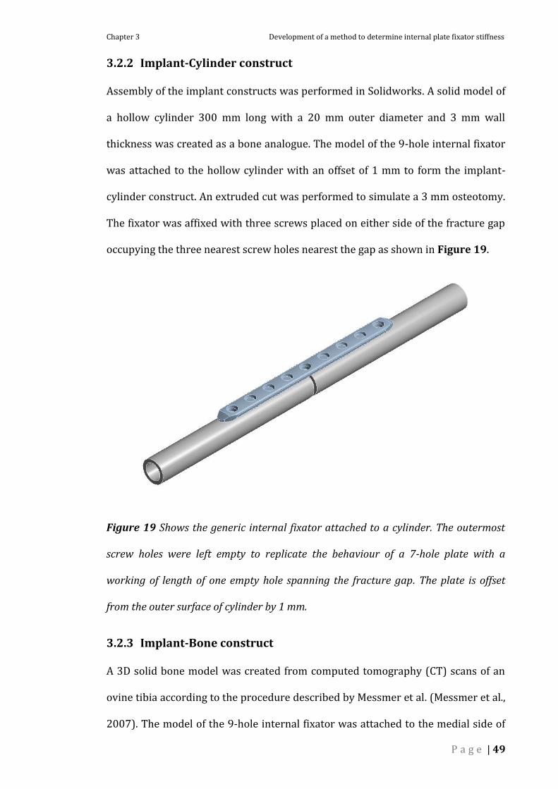
Chapter 3 Development of a method to determine internal plate fixator stiffness
P a g e | 49
3.2.2 Implant-Cylinder construct
Assembly of the implant constructs was performed in Solidworks. A solid model of
a hollow cylinder 300 mm long with a 20 mm outer diameter and 3 mm wall
thickness was created as a bone analogue. The model of the 9-hole internal fixator
was attached to the hollow cylinder with an offset of 1 mm to form the implant-
cylinder construct. An extruded cut was performed to simulate a 3 mm osteotomy.
The fixator was affixed with three screws placed on either side of the fracture gap
occupying the three nearest screw holes nearest the gap as shown in Figure 19.
Figure 19 Shows the generic internal fixator attached to a cylinder. The outermost
screw holes were left empty to replicate the behaviour of a 7-hole plate with a
working of length of one empty hole spanning the fracture gap. The plate is offset
from the outer surface of cylinder by 1 mm.
3.2.3 Implant-Bone construct
A 3D solid bone model was created from computed tomography (CT) scans of an
ovine tibia according to the procedure described by Messmer et al. (Messmer et al.,
2007). The model of the 9-hole internal fixator was attached to the medial side of

Chapter 3 Development of a method to determine internal plate fixator stiffness
P a g e | 50
the bone model at an offset of 3 mm to form the implant-bone construct (Figure
20). An extruded cut was performed to simulate a 3 mm mid diaphysis osteotomy.
The fixator was affixed with three screws placed on either side of the fracture gap
occupying the three screw holes nearest the gap.
Figure 20 Shows the generic internal fixator attached to an ovine tibia.
3.2.4 Creation of Finite Element (FE) model
A 3D finite element model was created for both the implant-cylinder and implant-
bone constructs (ANSYS Workbench 13, ANSYS, Inc, PA, USA). All structures were
described by linear elastic isotropic material properties. The implant material
(plate and locking screws) were made of stainless steel (E = 200 GPa, ν = 0.3).
Unlike implants which are made up of materials such as steel and have definite and
homogenous material properties throughout, living tissue such as bone are non-
homogenous and non-isotropic. Hence assigning material properties to bone is
more challenging. In the literature for such applications, assigning a single value
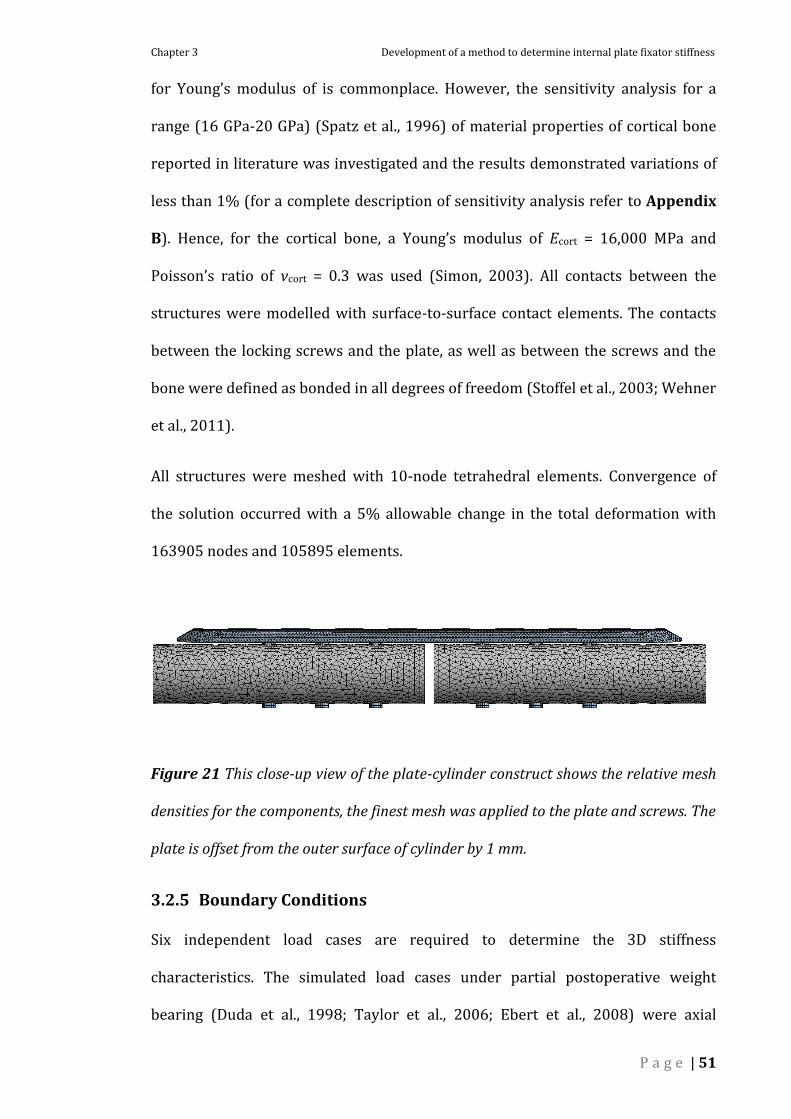
Chapter 3 Development of a method to determine internal plate fixator stiffness
P a g e | 51
for Young’s modulus of is commonplace. However, the sensitivity analysis for a
range (16 GPa-20 GPa) (Spatz et al., 1996) of material properties of cortical bone
reported in literature was investigated and the results demonstrated variations of
less than 1% (for a complete description of sensitivity analysis refer to Appendix
B). Hence, for the cortical bone, a Young’s modulus of Ecort = 16,000 MPa and
Poisson’s ratio of νcort = 0.3 was used (Simon, 2003). All contacts between the
structures were modelled with surface-to-surface contact elements. The contacts
between the locking screws and the plate, as well as between the screws and the
bone were defined as bonded in all degrees of freedom (Stoffel et al., 2003; Wehner
et al., 2011).
All structures were meshed with 10-node tetrahedral elements. Convergence of
the solution occurred with a 5% allowable change in the total deformation with
163905 nodes and 105895 elements.
Figure 21 This close-up view of the plate-cylinder construct shows the relative mesh
densities for the components, the finest mesh was applied to the plate and screws. The
plate is offset from the outer surface of cylinder by 1 mm.
3.2.5 Boundary Conditions
Six independent load cases are required to determine the 3D stiffness
characteristics. The simulated load cases under partial postoperative weight
bearing (Duda et al., 1998; Taylor et al., 2006; Ebert et al., 2008) were axial

Chapter 3 Development of a method to determine internal plate fixator stiffness
P a g e | 52
compression (400 N), torsion (5 Nm/degree), as well as bending (20 Nm/degree)
and shear (50 N) in both anterior-posterior and medial-lateral directions. The six
load cases were applied according to the boundary conditions described in
mechanical testing by both Kassi (Kassi et al., 2001)and Augat. (Augat et al., 2008)
in order to determine the effect of different boundary conditions reported in the
literature on the stiffness values calculated. In both the boundary conditions
suggested by Kassi and Augat, the distal/lower bone fragment was fixed firmly in
all DoFs (Degrees of Freedom). However, methods suggested by Kassi restricted
the lateral and rotational movements of the proximal/upper bone fragment, thus
creating both a confined axial compression and confined axial rotation.
Furthermore, while Augat applied four point bending, Kassi applied bending
moments to the top end of the proximal fragment. Also, shear loads were applied
as close to the fracture gap as possible using the BC (Boundary Condition)
suggested by Augat while Kassi applied shear force to the top end of the proximal
fragment. A third set of boundary conditions, referred to as the MPC (Multi Point
Constraint) boundary condition (Figure 22), was applied using a technique
specific to the finite element method that permitted the forces to be applied to
fracture fragments at the centre of the fracture gap using remote points rigidly
fixed to the upper and lower bone fragments. The boundary conditions
investigated are summarised in Figure 23.
To compare the stiffness values with the implant affixed to an anatomically
contoured bone and a simple cylinder model, the load cases were applied to both
constructs using the MPC boundary conditions described above. The individual
stiffness values in each of the six directions were compared.

Chapter 3 Development of a method to determine internal plate fixator stiffness
P a g e | 53
Figure 22 Schematic shows the MPC boundary condition. (DoFs = Degrees of
Freedom).

Chapter 3 Development of a method to determine internal plate fixator stiffness
P a g e | 54
Figure 23 Schematic shows the boundary conditions employed in each of the load
cases as defined by Kassi et al and Augat et al as well as the for the application of
loads via MPC ( or represents DoFs fixed in all 6 directions and represents
restricted lateral and rotational movements).

Chapter 3 Development of a method to determine internal plate fixator stiffness
P a g e | 55
3.2.6 Analysis
The translational inter-fragmentary movements were determined from the
displacement of a node positioned at the centre of the fracture gap attached to the
upper fragment relative to a coincident node attached to the lower fragment. The
rotational inter-fragmentary movements were calculated using matrix algebra. For
a complete description of the inter-fragmentary movements calculation procedure,
refer to Appendix A. The orientation of each bone fragment was defined by a local
coordinate system defined by three nodes on each body (proximal and distal
fragments). The rotational transformation from one fragment into the other was
then calculated and decomposed into angles about the three coordinate axes.
The individual stiffness for each of the six load cases was determined by equating
the applied load to the IFM in the direction of load application.
x
xx
U
F=K , where x denotes the direction of load application
A complete 6 by 6 stiffness matrix (below) was calculated by relating the three
forces (Fx, Fy, Fz, forces in the x, y and z directions) and three moments (Mx, My, Mz,
moments about the x, y and z axes) applied in each of the six independent load
cases and the resulting inter-fragmentary movements (ux, uy, uz translations in x, y,
and z and α, β, γ rotations about x, y, and z) as described by Duda et al., 1998 (Duda
et al., 1997).
The diagonal values of the stiffness matrix (S11, S22..., S66) correspond to the
stiffness in the principal directions (i.e. S11 = anterior-posterior shear, S22 = medial-
lateral shear, S33 = axial compression, S44 = medial-lateral bending, S55 = anterior-
posterior bending, S66 = axial torsion).

Chapter 3 Development of a method to determine internal plate fixator stiffness
P a g e | 56
z
y
x
z
y
x
M
M
M
F
F
F
666564636261
565554535251
464544434241
363534333231
262524232221
161514131211
SSSSSS
SSSSSS
SSSSSS
SSSSSS
SSSSSS
SSSSSS
*
z
y
x
U
U
U
3.3 Results
The inter-fragmentary movements and values for each of the six stiffness
components are listed in Table 1 for the different boundary conditions
investigated. The stiffness values calculated were varied depending on the method
of calculation; stiffness matrix versus individual and with the boundary conditions
applied.
The stiffness matrix method determined substantially different stiffness values for
axial compression, torsion, anterior-posterior and medial-lateral bending and
anterior-posterior shear. There was no difference in the medial-lateral shear
between the two methods (Augat and Kassi). Values determined via the stiffness
matrix method tended to be higher, in some cases many orders of magnitude
higher (axial compression stiffness determined using Kassi boundary conditions
equals 147000 versus 4444 N/mm) than the values determined using individual
stiffness calculation method. This trend was observed with all three sets of
boundary conditions.
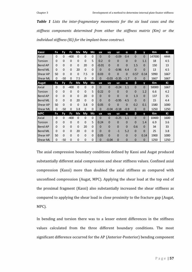
Chapter 3 Development of a method to determine internal plate fixator stiffness
P a g e | 57
Table 1 Lists the inter-fragmentary movements for the six load cases and the
stiffness components determined from either the stiffness matrix (Km) or the
individual stiffness (Ki) for the implant-bone construct.
The axial compression boundary conditions defined by Kassi and Augat produced
substantially different axial compression and shear stiffness values. Confined axial
compression (Kassi) more than doubled the axial stiffness as compared with
unconfined compression (Augat, MPC). Applying the shear load at the top end of
the proximal fragment (Kassi) also substantially increased the shear stiffness as
compared to applying the shear load in close proximity to the fracture gap (Augat,
MPC).
In bending and torsion there was to a lesser extent differences in the stiffness
values calculated from the three different boundary conditions. The most
significant difference occurred for the AP (Anterior-Posterior) bending component
Kassi Fx Fy Fz Mx My Mz ux uy uz α β γ Km Ki
Axial 0 0 -400 0 0 0 0 0 -0.09 0.4 0 0 147000 4444
Torsion 0 0 0 0 0 5 0.2 0 0 0 0 1.1 18 4.5
Bend AP 0 0 0 0 20 0 -0.01 0 0 0 1.5 0 150 13
Bend ML 0 0 0 20 0 0 0 0 -0.96 4.4 0 0 13 4.5
Shear AP 50 0 0 0 7.5 0 0.03 0 0 0 0.57 0.14 5990 1667
Shear ML 0 -50 0 7.5 0 0 0 -0.03 -0.35 -1.7 0 0 1667 1667
Augat Fx Fy Fz Mx My Mz ux uy uz α β γ Km Ki
Axial 0 0 -400 0 0 0 0 0 -0.24 1.1 0 0 50000 1667
Torsion 0 0 0 0 0 5 0.22 0 0 0 0 1.2 6.6 4.2
Bend AP 0 0 0 0 20 0 0 0 0 0 1.3 0 137 15
Bend ML 0 0 0 20 0 0 0 0 -0.95 4.5 0 0 15 4.4
Shear AP 50 0 0 0 3.8 0 0.05 0 0 0 0.2 0.1 1580 1000
Shear ML 0 -50 0 3.8 0 0 0 -0.04 -0.18 -0.9 0 0 1250 1250
MPC Fx Fy Fz Mx My Mz ux uy uz α β γ Km Ki
Axial 0 0 -400 0 0 0 0 0 -0.25 1.1 0 0 10400 1600
Torsion 0 0 0 0 0 5 0.24 0 0 0 0 1.4 6.9 3.6
Bend AP 0 0 0 0 20 0 0 0 0 0 0.6 0 34 33
Bend ML 0 0 0 20 0 0 0 0 -1 5.2 0 0 25 3.8
Shear AP 50 0 0 0 0 0 0.05 0 0 0 0 0.14 1900 1000
Shear ML 0 -50 0 0 0 0 0 -0.04 0 0 0 0 1250 1250

Chapter 3 Development of a method to determine internal plate fixator stiffness
P a g e | 58
calculated from the MPC boundary condition. The MPC boundary condition led to a
significantly higher AP bending stiffness than both the Kassi and Augat BCs.
Figure 24 Shows the stiffness components determined for each of the three
investigated boundary conditions using implant-cylinder construct.
The stiffness characterisation of fixation devices may be performed with the
fixation construct attached to a bone or bone substitute such as a hollow cylinder
of artificial material. Comparing the stiffness values obtained, it was found that the
geometry of the bone analogue influenced axial stiffness the most.
0
10
20
30
40
0
1000
2000
3000
4000
5000
Sti
ffn
ess
(N
m/
de
g)
Sti
ffn
ess
(N
/m
m)
Kassi Augat MPC
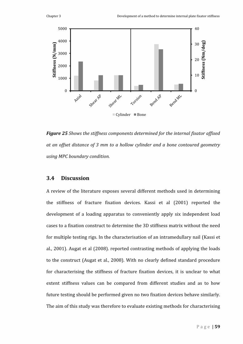
Chapter 3 Development of a method to determine internal plate fixator stiffness
P a g e | 59
Figure 25 Shows the stiffness components determined for the internal fixator affixed
at an offset distance of 3 mm to a hollow cylinder and a bone contoured geometry
using MPC boundary condition.
3.4 Discussion
A review of the literature exposes several different methods used in determining
the stiffness of fracture fixation devices. Kassi et al (2001) reported the
development of a loading apparatus to conveniently apply six independent load
cases to a fixation construct to determine the 3D stiffness matrix without the need
for multiple testing rigs. In the characterisation of an intramedullary nail (Kassi et
al., 2001). Augat et al (2008). reported contrasting methods of applying the loads
to the construct (Augat et al., 2008). With no clearly defined standard procedure
for characterising the stiffness of fracture fixation devices, it is unclear to what
extent stiffness values can be compared from different studies and as to how
future testing should be performed given no two fixation devices behave similarly.
The aim of this study was therefore to evaluate existing methods for characterising
0
10
20
30
40
0
1000
2000
3000
4000
5000
Sti
ffn
ess
(N
m/
de
g)
Sti
ffn
ess
(N
/m
m)
Cylinder Bone

Chapter 3 Development of a method to determine internal plate fixator stiffness
P a g e | 60
the stiffness of fracture fixation devices and define an appropriate protocol for
evaluating the stiffness of an internal fixator.
3.4.1 Method of stiffness calculation
Stiffness is the relationship between force and displacement. For any single
direction, i.e. axial compression, the stiffness can be calculated by relating the
displacement in the direction of loading to the applied force. A three-dimensional
stiffness matrix can also be calculated to represent the stiffness behaviour of a
body or construct. A significant discrepancy was found for the stiffness values for
an internal fixator using the two different methods. The differences appear
attributable to the fact that the internal fixator does not undergo six unique
displacement modes under the six load cases. The deformation behaviour under an
axial compressive load and ML (Medial-Lateral) bending load are very similar, both
result in axial compression and ML bending at the fracture gap. Similarly, axial
torsion and anterior-posterior shear resulted in similar IFM’s. Because of the
position of the fixator relative to the long axis of the bone, eccentric loading is
created and asymmetric deformation results. For example, AP shear loading not
only produces an IFM in the AP direction but also results in an axial torsion
moment about the fixator it produces additional torsional deformation. As these
additional moments are not accounted for in the force matrix, this leads to errors
in the calculation of the stiffness components.
Moreover, when investigated in detail, it was surprising to know that even a slight
change to IFM’s of the order of 0.01 mm (especially in axial inter-fragmentary
movement for the ML bending load case) resulted in a huge difference in stiffness
value. The Figure 26 highlights the sensitivity of stiffness values to slight changes
in certain IFM’s. Hence, it was concluded that the stiffness matrix is highly

Chapter 3 Development of a method to determine internal plate fixator stiffness
P a g e | 61
sensitive and even small amounts of error in determination of IFM of the order of
0.01 of a millimetre would result in huge differences in the calculated fixation
stiffness value.
Figure 26 Shows the axial compressional stiffness value determined via stiffness
matrix method for different axial IFM’s (-0.69 mm - -0.73 mm) for the medial-lateral
bending load case.
Therefore, the stiffness components in each direction were determined by relating
the applied force in each direction to the resulting displacement in that direction
(individual stiffness calculation method).
3.4.2 Boundary Conditions for stiffness determination
In both the boundary conditions adopted by Augat and Kassi for the determination
of axial compressive stiffness and torsional stiffness, the bone fixator construct
was held fixed at the bottom and load applied to the top end of the proximal
fragment. The BC’s did differ however in the constraints applied to the upper
fragment. The testing-rig proposed by Kassi restricts horizontal motion and
rotation of the upper fragment and so creates both a confined axial compression

Chapter 3 Development of a method to determine internal plate fixator stiffness
P a g e | 62
and confined axial torsion. Augat on the other hand employed a universal/cardan
joint to enable free rotation of the construct at the upper support. Determination of
the axial stiffness under confined compression led to significantly higher values
than under unconfined compression. Due to the position of the internal fixator
relative to the loading axis, this eccentric loading results primarily in a ML bending
deformation mode rather than a uniform axial compression. Because the confined
compression restricts the bending of the construct, the IFM is restricted and hence
higher stiffness results. In this study, the effect of confining the upper fragment
was less prevalent on the torsional stiffness. However, for more complicated
geometries, i.e. where stiffness determination is performed on a fixator attached to
a contoured bone, a more complicated deformation pattern may result and
stiffening occur due to restriction of movement.
In respect to the application of shear loads, there are also substantial differences
between the BC’s applied by Kassi and Augat. Kassi’s rig uses the rotation of biaxial
materials testing machine to apply a lateral load to top of the construct, whereas
Augat firmly grips both fragments, one is fixed and the other is attached to the
actuator of the materials testing machine. In applying the shear load to the top of
the construct, which is weakest in the middle section, the deformation mode is
more akin to bending rather than shear. The shear stiffness is also overestimated
relative to the situation where the loads are applied closer to the fracture gap
because, as the fragment bends relative to lower fragment, a fracture gap
displacement occurs in the opposite direction to loading. The resulting shear IFM
is thus equal to the shear IFM less the IFM in the opposite direction due to bending.
Applying the loads closer to the fracture gap reduces the lever arm of the load and
hence the moment and ultimately the bending.

Chapter 3 Development of a method to determine internal plate fixator stiffness
P a g e | 63
Despite differences in the shear stiffness determined applying the different BCs
(Boundary Conditions); the shear movements themselves were very small, of the
order of less than 0.05 mm. This is both attributable to the BCs themselves with
induced bending rather than pure shear, but also the nature of the internal fixation
device itself, that through its close proximity to the bone permits very little shear
movement. In this study, a relatively stiff internal fixator configuration was tested
with a short working length of one hole. Shear movements may be greater with
differently configured plates and the influence of internal fixator configuration on
the stiffness components is subject of a separate study (refer to Chapter 4).
The application of BC for the case of bending loads varied between the different
BC’s investigated. While Kassi held the bone-fixator construct fixed at the bottom
and applied bending moments to the top end of the upper fragment, Augat applied
4 point bending (Figure 23). On the other hand, using MPC BC, bending moments
were applied to the node forming centre of fracture gap connected to the proximal
fragment while a coincident node connected to the distal fragment was fixed in all
DoFs. Investigation of the effect of BC on bending stiffness showed that the
bending stiffness in anterior-posterior direction determined using MPC BC was
double the stiffness value determined using either Kassi or Augat BC’s. Since the
centre node connected to the distal fragment is fixed in all DoFs, it is restricted
from bending and hence a higher bending stiffness of the construct. Although
applying BC as suggested by Augat (four point bending) resulted in a more uniform
bending of the construct, applying four point bending to a bone-implant construct
may not be feasible due to the complex geometry of the bone. Hence, for purposes
of parameter analysis, the use of MPC BC may be appropriate while investigating
the effect of bending loads on implant stability.

Chapter 3 Development of a method to determine internal plate fixator stiffness
P a g e | 64
3.4.3 Bone contoured geometry versus simple cylinder
Methods of stiffness determination also vary in the use of bone analogues. Whilst
some studies used cadaveric bones, others used artificial bones or hollow cylinders
to represent bone. In this study, the influence of contoured bone geometry versus a
simple cylinder was investigated. The geometry of the bone analogue did influence
the stiffness components and to varying degrees, in this case, axial stiffness was
affected the most. Using the finite element method, all other variables (material
properties, interface properties, etc) were held constant. Therefore, the differences
determined here can be attributed to the effect of geometry alone. The reason for
the differences can be attributed to differences in offset between fixator and the
bone; the contoured bone shape dictates the plate be placed a greater distance
from the bone, the bone axis is also curved which gives rise to differences In some
cases, the use of a bone contoured geometry may be dictated by the question
addressed in a particular study, however a simple cylindrical geometry can be used
for stiffness determination and enhance comparison between the results of
different studies.
This study has few limitations and assumptions which should be discussed. The
cortical bone was simplified and described as a homogenic material with linear
elastic and isotropic material properties. Due to the presence of segmental defect,
it is expected that most of the load transfer happens through the fixator and the
bone acts very similar to a rigid body. Hence, we believe assigning a single value
for material property would not alter the fixation stiffness value determined.
However, sensitivity analysis performed demonstrated that the variations to the
value of young’s modulus of the cortical ovine tibia in the range 14 GPa- 24 GPa
(Spatz et al., 1996) reported in literature led to differences in calculated axial

Chapter 3 Development of a method to determine internal plate fixator stiffness
P a g e | 65
compressional stiffness value of up to a maximum of 1 % (refer to Appendix B).
Hence, the simplified description of the bone material was assumed to be
uncritical.
In the model created for this project, forces were applied to an artificially
constructed conical extension to the bone within the fracture gap (imaginary point
representing the centre of the fracture gap connected to the fracture fragments
(proximal and distal) via rigid beam elements (Multi-Point Constraint (MPC))).
Hence, the deformation at the osteosynthesis and thus the determined stiffness
matrix will also be influenced by the local deformation of the bone fragments and
of the conical extension (rigid beam) apart from the deformations of the fixator.
However, the results showed that the deformation of the bone and the rigid beams
were less than 0.01 mm suggesting that they behaved very similar to a rigid body.
Therefore, the application of forces to this conical extension was assumed not to
alter the determined fixation stiffness.
In this study, the perfectly modelled screw-bone and screw-plate interface could
over estimate the stiffness values determined. However, the FE model was
compared with results from mechanical testing (For a complete description of the
FEA model comparison process, refer to Appendix C). Although there were
differences in absolute values between FEA and mechanical testing results, similar
deformation behaviour was observed between FEA and mechanical tests for the
two fixator screw configurations investigated which to an extent verifies the FE
model. Besides, since relative comparison (effect of different boundary conditions
on fixation stiffness) is performed in this study, determination of absolute values is
not essential. Hence, the assumption of perfectly modelled screw-bone or screw-
plate interface was assumed to be not critical.

Chapter 3 Development of a method to determine internal plate fixator stiffness
P a g e | 66
3.5 Conclusion
In summary, this study highlighted the importance of input parameters such as
boundary conditions and method of stiffness calculation on fixation stiffness. After
having analysed different methods previously used in literature, it was concluded
that the method of applying loads to the centre of fracture gap as explained in MPC
BC to be a convenient method to determine internal plate fixation stiffness using
FE technique. In addition, owing to the highly sensitive nature of stiffness matrix, a
decision to use the individual stiffness calculation method for internal fixation
stiffness determination was made.

P a g e | 67
4 Investigation of the influence of fixator
configuration on fixation stiffness
This chapter focuses on determining the influence of fixator configuration on
fixation stability using methods developed in Chapter 3 of this thesis.

Chapter 4 Investigation of the influence of fixator configuration on fixation stiffness
P a g e | 68
4.1 Introduction
The influence of mechanics on the healing outcome of bone fractures is well
documented. The local mechanical conditions are determined by limb-loading and
the stability of fixation. A range of fixation devices are available for the treatment
of bone fractures and choice depends on the location and the severity of the
fracture.
Locked plating constructs also referred to as internal fixation devices have been
developed with the goal of biologic fixation in mind. Used as a bridging construct,
internal fixation devices are intended to provide flexible fixation to support repair
via the secondary bone healing pathway with callus formation. The locking screws
allow the fragments to be stabilised without compressing the fixator onto the bone
surface, thereby preserving the peripheral blood supply to the bone. Recent
developments in surgical techniques have also enabled these devices to be applied
in a minimally-invasive approach causing less disruption to the injured tissues.
Internal fixation devices have also been shown to provide improved fixation
strength in osteoporotic bone (Henderson et al., 2011). These benefits of internal
plate fixation have led to rapid adoption of this technology.
Recent biomechanical studies suggest however, that internal fixation devices
(Locking plates) may be overly stiff when compared to external fixators and
suppress inter-fragmentary motion to a level that may be insufficient to reliably
promote secondary bone healing (Bottlang et al., 2010; Bottlang and Feist, 2011).
Due to the proximity of the plate to the cortex, movements at the near cortex are
again a fraction of those at the far cortex raising further concern that excessive
stiffness may prevent stimulation of callus formation. Recent clinical studies

Chapter 4 Investigation of the influence of fixator configuration on fixation stiffness
P a g e | 69
confirm that the inherently high construct stiffness of locked-plate constructs
suppresses callus formation (Bottlang et al., 2010; Bottlang and Feist, 2011).
There are no clear guidelines as to the stiffness requirements for fixation devices
because all fractures are not created equal. Therefore for the same fixation
stiffness, the inter-fragmentary motion in the fracture gap will vary depending on
limb loading and the size of the fracture gap. Furthermore, fixation devices are
highly non-linear in the sense that axial load does not translate purely into axial
inter-fragmentary motion but rather a combination of axial, shear and bending
displacements. Studies investigating the influence of micro-motion on healing have
demonstrated that axial inter-fragmentary movements of the order of 0.2 – 1 mm
in a 3 mm osteotomy gap provide best healing outcome in sheep where simple
diaphyseal long bone fracture stabilised with a custom made external ring fixator
was investigated (Claes et al., 1998). Furthermore, fixation devices that provide a
high resistance to shear and torsional movements but enable a moderate amount
of axial inter-fragmentary movement have been shown to provide timely healing
with callus formation in animal studies (Epari et al., 2007).
There is no single one way to configure an internal fixation device. Choices
available to the surgeon include the length and size of the plate, the material, the
number and configuration of the screws. The parameters which influence internal
fixator stiffness are the material properties, the cross-section or shape of the
fixator, effective plate length, the offset distance from the underside of the fixator
to the bone surface, number and position of screws, and the screw type. However,
it is unclear how all these different parameters affect the fixation stability and
whether they can be manipulated to optimise the mechanical conditions for
healing. Therefore, the purpose of this study is to characterise the fixation

Chapter 4 Investigation of the influence of fixator configuration on fixation stiffness
P a g e | 70
stability of an internal plate fixation device and the influence of modifications
to its configuration on implant stability.
While the motivation of the study is configuration of internal plate fixation devices
for optimal stability (moderate axial inter-fragmentary movements with high
resistance to shear and torsional movements), the hypothesis of the study is that
the internal fixation devices are inherently too stiff so as to promote sufficient
callus formation for better healing outcome. In this study, characterisation of
fixation stiffness of internal plate fixator will be performed using MPC (Multi Point
Constraint) boundary condition where loads and boundary conditions will be
applied to the node forming the centre of fracture gap in FE. Simplified bone
geometry (cylinder) with a 3 mm mid shaft osteotomy on to which a generic 9 hole
locking plate is attached will be used in the analysis. Specifically, the current study
is designed to investigate the influence of modifications to fixator configurations
on implant stability. The fixator configurations chosen for analysis are fixator
material properties (Stainless Steel and Titanium), fixator offset (1 and 3 mm),
fixator inclination (+ and -0.75 degrees), screw configuration (Working length
(distance between the inner most screws), screw spacing, number of screws and
effective plate length). The fixator configuration in terms of material of the fixator
was dictated by the material of the commercially available implants.
The knowledge gained through this analysis is expected to prove useful in
providing a guideline in the configuration of internal plate fixators that allow
moderate axial IFM at the fracture site for sufficient callus formation.
Chapter 4 Investigation of the influence of fixator configuration on fixation stiffness
P a g e | 71
4.2 Materials and methods:
4.2.1 Internal fixator
A generic locked plating implant was created (Solidworks 2010, Dassault
Systèmes, Massachusetts, USA) to closely represent a standard 9-hole 4.5 mm
osteosynthesis plates and screws that are commercially available from several
manufacturers. The plate was 170 mm long, 13.5 mm wide and 4.5 mm thick.
4.2.2 Implant-Bone analogue construct
In the standard configuration the plate was attached to a hollow cylinder with an
outer diameter of 20 mm and wall thickness of 3 mm that represented cortical
bone in diaphysis of a long bone (tibia). Six screws, three in each fragment, were
used to attach the plate to the bone utilising the three innermost screw holes on
each side of the simulated osteotomy (0xxx0xxx0, where empty screw holes are
represent by a “0” and filled holes by a “x”). The standard screw configuration is
shown in Figure 27.

Chapter 4 Investigation of the influence of fixator configuration on fixation stiffness
P a g e | 72
Figure 27 Internal fixator and bone cylinder construct in the standard configuration
(0xxx0xxx0) for an effective plate length of 7-hole with three screws on either side of
the osteotomy gap.
4.2.3 Finite element model
A finite element model of the implant-bone construct was generated in ANSYS 13,
(ANSYS, Inc., Canonsburg, PA, USA) by importing a parasolid file of the implant-
bone solid model.
All structures were meshed with 10-node tetrahedral elements with an assigned
element size for each component.
All structures were described by linear elastic isotropic material properties. For
the cortical bone, a Young’s modulus of Ecort = 16,000 MPa and Poisson’s ratio of
νcort = 0.3 was used. The implant material (plate and locking screws) were made of

Chapter 4 Investigation of the influence of fixator configuration on fixation stiffness
P a g e | 73
either stainless steel (SS) (Ess = 200,000 MPa, νss = 0.3) or titanium alloy (Ti) (ETi =
110,000 MPa, νTi = 0.33).
All contacts between the structures were modelled with surface-to-surface contact
elements. The contacts between the locking screws and the plate, as well as
between the screws and the bone were defined as bonded in all degrees of freedom
(DoFs).
For the application of boundary conditions, two coincident nodes were modelled in
the middle of the fracture gap, which were connected to the outer ends of the bone
fragments at the fracture site using rigid beam elements. The node connected to
the distal bone fragment was fixed in all six DoFs. At the proximal node the loads
for the different load cases used in the stiffness determination were applied.
4.2.4 Stiffness determination
The stiffness of the constructs was determined in all six directions (axial
compression and axial torsion, medial-lateral (ML) bending and anterior-posterior
(AP) bending and ML and AP shear). The loads applied in each direction were axial
compression (400 N), axial torsion (5 N/m), medial-lateral and anterior-posterior
bending (20 N/m) and medial-lateral and anterior-posterior shear (50 N). The
inter-fragmentary movements (IFM) (all three translations) were determined from
the node at the centre of the fracture gap and additionally the axial IFM at the near
and far cortex to the plate were determined from nodal displacements (Figure
28). The bending and rotational displacement components were from
displacement of the proximal fragment using matrix algebra. The detailed
description of the calculation procedure can be found in Appendix A.

Chapter 4 Investigation of the influence of fixator configuration on fixation stiffness
P a g e | 74
Figure 28 Illustration of calculation of axial component of IFM (Inter Fragmentary Movement)
using MPC (Multi Point Constraint) BC (Boundary Condition).
4.2.5 Configurations
To determine those parameters that have the greatest influence on internal plate
fixation stability a number of different configurations were investigated. The
material properties of the plate and screws were simulated as Stainless Steel or
Titanium (internal plate fixators are generally available in these two materials).
The distance between the plate and the bone (plate offset) was varied between 1
and 3 mm, the inclination of the plate was varied between +0.75 and -0.75 degrees
(maximum inclination achieved before plate contacted the bone surface for a 1 mm
offset distance between plate and bone) to the bone. Screw configuration was
altered varying the working length (distance between innermost screws), the
effective plate length, the screw spacing and the screw number. The screw

Chapter 4 Investigation of the influence of fixator configuration on fixation stiffness
P a g e | 75
configurations investigated are detailed in Figure 29. Finally, the effect of bi-
cortical and far cortical screw anchorage was examined. Far-cortical locking
(Figure 31) was simulated in the finite element model by removing the contact
surfaces on the near cortex. No inhibition of movement by the near cortex was
permitted, allowing determination of stiffness of fixation prior to screw contact
with the screw-hole wall on the near cortex.
Figure 29 Schematic representation of the screw configurations investigated.
(Notation: e.g. Top left 0XXX0XXX0, Top right X0XX0XX0X).
Figure 30 Shows a generic locking plate (modified from 9 hole, 4.5 mm standard
Locking Compression Plate) with three screws on either side of the fracture gap
leaving the middle screw hole empty.
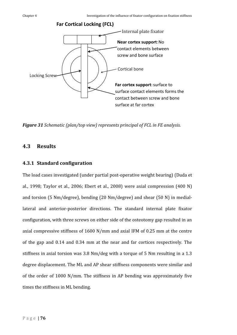
Chapter 4 Investigation of the influence of fixator configuration on fixation stiffness
P a g e | 76
Figure 31 Schematic (plan/top view) represents principal of FCL in FE analysis.
4.3 Results
4.3.1 Standard configuration
The load cases investigated (under partial post-operative weight bearing) (Duda et
al., 1998; Taylor et al., 2006; Ebert et al., 2008) were axial compression (400 N)
and torsion (5 Nm/degree), bending (20 Nm/degree) and shear (50 N) in medial-
lateral and anterior-posterior directions. The standard internal plate fixator
configuration, with three screws on either side of the osteotomy gap resulted in an
axial compressive stiffness of 1600 N/mm and axial IFM of 0.25 mm at the centre
of the gap and 0.14 and 0.34 mm at the near and far cortices respectively. The
stiffness in axial torsion was 3.8 Nm/deg with a torque of 5 Nm resulting in a 1.3
degree displacement. The ML and AP shear stiffness components were similar and
of the order of 1000 N/mm. The stiffness in AP bending was approximately five
times the stiffness in ML bending.

Chapter 4 Investigation of the influence of fixator configuration on fixation stiffness
P a g e | 77
4.3.2 Internal fixator material properties
Table 2 The effect of implant material properties on the stability of internal plate
fixation.
0xxx0xxx0 (SS) 0xxx0xxx0 (Ti)
%
reduction
in stiffness
Stiffness IFM (mm) Stiffness IFM (mm)
Axial (N/mm) 1600 0.25 (0.14-0.34) 900 0.44 (0.26-0.61) 44
Torsion (Nm/deg) 3.8 1.3 2.3 2.2 36
Bend AP (Nm/deg) 33 0.6 20 1.0 39
Bend ML (Nm/deg) 4.0 5.0 2.4 8.4 40
Shear AP (N/mm) 1000 0.05 715 0.07 29
Shear ML (N/mm) 1250 0.04 830 0.06 34
Changing the implant material from stainless steel to titanium led to a 29 - 44%
reduction in the stiffness components, the greatest reduction occurred in the axial
direction (44%).
4.3.3 Internal fixator offset
Table 3 The effect of implant offset to the bone on the stability of internal plate
fixation.
0xxx0xxx0 1mm offset 0xxx0xxx0 3mm offset
% reduction
in stiffness
Stiffness IFM (mm) Stiffness IFM (mm)
Axial (N/mm) 1600 0.25 (0.14-0.34) 1210 0.33 (0.10-0.56) 24
Torsion (Nm/deg) 3.6 1.4 3.1 1.6 14
Bend AP (Nm/deg) 33 0.6 28 0.7 15
Bend ML (Nm/deg) 4.0 5.0 4.0 5.0 0
Shear AP (N/mm) 1000 0.05 830 0.06 17
Shear ML (N/mm) 1250 0.04 1250 0.04 0

Chapter 4 Investigation of the influence of fixator configuration on fixation stiffness
P a g e | 78
Increasing the offset between the internal fixator and the bone resulted in a
decrease in construct stiffness, however not all stiffness components were affected
equally. No significant changes (see IFMs) were determined in either the ML or AP
bending or shear components. The greatest reduction occurred in the axial
direction (24%).
4.3.4 Internal fixator inclination
Table 4 The effect of implant inclination to the bone on the stability of internal plate
fixation.
0xxx0xxx0 0xxx0xxx0 +/- incl
% reduction
in stiffness
Stiffness IFM (mm) Stiffness IFM (mm)
Axial (N/mm) 1600 0.25 (0.14-0.34) 1540 0.26 (0.07-0.44) 4
Torsion (Nm/deg) 3.8 1.3 5 1 -32
Bend AP (Nm/deg) 33 0.6 40 0.5 -21
Bend ML (Nm/deg) 4 5 4.9 4.1 -23
Shear AP (N/mm) 1000 0.05 1670 0.03 -67
Shear ML (N/mm) 1250 0.04 1670 0.03 -34
Placing the internal fixator at either a positive or negative inclination to the axis of
the bone and hence the loading direction had no significant effect on the axial IFM
at the centre of the gap and hence the axial stiffness. However the axial IFM at the
far cortex was increased by 29% and at the near cortex it decreased by 50%.
Contrary to the axial stiffness, the remaining stiffness components increased by
between 20 - 65% with AP shear most affected. There was no difference between
either the positive or negative inclination.

Chapter 4 Investigation of the influence of fixator configuration on fixation stiffness
P a g e | 79
4.3.5 Screw configuration
Table 5 The effect of working length on the stability of internal plate fixation.
0xxx0xxx0 xxx000xxx
%
reduction
in stiffness
Stiffness IFM (mm) Stiffness IFM (mm)
Axial (N/mm) 1600 0.25 (0.14-0.34) 850 0.47 (0.10-0.83) 47
Torsion (Nm/deg) 3.6 1.4 2.3 2.2 36
Bend AP (Nm/deg) 33 0.6 20 1.0 39
Bend ML (Nm/deg) 4 5 2.2 9.2 45
Shear AP (N/mm) 1000 0.05 415 0.12 59
Shear ML (N/mm) 1250 0.04 225 0.22 82
Increasing the working length and the effective plate length, but keeping the
number of screws per fragment constant, resulted in a significant decrease in all
stiffness components (>40%). The largest decrease in stiffness occurred in the ML
shear direction (82%). Changing the working length by one empty screw hole i.e.
from xxx0xxx to xxx00xxxx decreased the axial stiffness by 30% when compared to
by two holes which decreased the stiffness by 47%.
Table 6 The effect of working length on the stability of internal plate fixation.
0xxx0xxx0 xx0x0x0xx
% reduction
in stiffness
Stiffness IFM (mm) Stiffness IFM (mm)
Axial (N/mm) 1600 0.25 (0.14-0.34) 1600 0.25 (0.06-0.46) 0
Torsion (Nm/deg) 3.6 1.4 3.3 1.5 13
Bend AP (Nm/deg) 33 0.6 33 0.6 0
Bend ML (Nm/deg) 4 5 3.7 5.4 8
Shear AP (N/mm) 1000 0.05 1000 0.05 0
Shear ML (N/mm) 1250 0.04 1250 0.04 0

Chapter 4 Investigation of the influence of fixator configuration on fixation stiffness
P a g e | 80
Increasing the plate length but keeping the working length the same had little
effect on the stiffness of the construct. Similarly, altering the spacing of the screws
from xx0x0x0xx to x0xx0xx0x and xx0x0x0xx to xxxx0xxxx had only minor effects
on the stiffness of the construct.
4.3.6 Far cortical locking
Table 7 The effect of bi-cortical versus far cortical locking on the stability of internal
plate fixation.
0xxx0xxx0 0xxx0xxx0 FCL
%
reduction
in stiffness
Stiffness IFM (mm) Stiffness IFM (mm)
Axial (N/mm) 1600 0.25 (0.14-0.34) 1170 0.34 (0.15-0.53) 27
Torsion (Nm/deg) 3.8 1.3 1.9 2.6 50
Bend AP (Nm/deg) 33 0.6 10 2.0 70
Bend ML (Nm/deg) 4 5 3.6 5.5 10
Shear AP (N/mm) 1000 0.05 450 0.11 55
Shear ML (N/mm) 1250 0.04 1000 0.05 20
Far cortical locking has been proposed as a new design to conventional internal
plate fixation devices to reduce construct stiffness. Far cortical locking led to a
27% reduction in axial stiffness but also over 50% reductions in torsion and AP
shear and bending stiffness. In contrast, to modifications to the working length
which decreased motion at the near cortex, far cortical locking increased axial IFM
at both the near and far cortex (Compare Table 5 and Table 7).
4.4 Discussion
Recent clinical and biomechanical studies have suggested that internal fixation
devices may be too stiff to reliably stimulate callus formation. Furthermore, timely

Chapter 4 Investigation of the influence of fixator configuration on fixation stiffness
P a g e | 81
healing has been shown to require a moderate axial stiffness and high stiffness in
the shear and torsional directions. In this study, a 3D finite element model was
used to characterise the stiffness of an internal plate fixator. An internal fixator
configured with an offset of 1 mm to the bone surface and three screws on either
side of the fixator made of stainless steel was found to exhibit high stiffness,
particularly against shear. The axial IFM at the near cortex under a load equivalent
to partial weight bearing was extremely low (0.05 mm). Modifications to the model
were then made to investigate the influence of changes to internal plate fixation
configuration on its stiffness components to determine the most appropriate
method to increase the flexibility of fixation and to control the axial IFM.
Internal plate fixation devices are available from most manufacturers in either
stainless steel or titanium. As expected, a change in material property from
stainless steel to titanium resulted in a decrease in stiffness by almost 50%,
equivalent to the difference in elastic modulus between the two materials. Due to
the complex non-linear nature of the bone fixator construct the change in material
properties did not influence all stiffness components equally. The change
influenced the axial, ML bending and torsional stiffness components to the greatest
extent. Although a 30% decrease in shear stiffness was determined, the shear
movements with both steel and titanium plates were insignificant (less than 0.1
mm). The axial IFM at the near cortex increased substantially from 0.14 to 0.26
mm (86%).
In the case of external fixation devices the distance between the plate and the bone
has a considerable influence on the overall construct stability. In contrast to
external fixation, the free bending length of the screws is considerably less with
internal fixation as the internal fixator is placed in close proximity to the bone

Chapter 4 Investigation of the influence of fixator configuration on fixation stiffness
P a g e | 82
under the muscle/skin. In internal fixation the plate should be held at a distance
slightly away from the bone to preserve the peripheral blood supply to the bone. In
this study we investigated influence of offset by increasing the offset between the
plate and the bone from 1 mm up to a conceivable 3 mm. Increasing plate offset by
2 mm reduced axial and torsional stiffness by approximately 20-25%, however
there was no influence on the bending stiffness and the magnitude of the shear
movements remained insignificant. The irregular geometry of the bone may also
dictate that the plate is placed at an inclination to the long axis and hence the
direction of loading. In this study, placing the plate at an inclination to the bone
had almost no effect on the axial stiffness but surprisingly increased the remaining
stiffness components. The change in stiffness was the same whether the plate was
inclined positively or negatively from the bone axis.
The screw configuration is known to influence not only the stability of internal
fixation but also the stresses within the plate and likelihood of plate failure. In a
previous study the influence of screw configuration on the axial and torsional
stiffness was investigated with the finding that the working length, the distance
between the innermost screws on either side of the fracture gap, is the greatest
determinant of construct stiffness and that more than three screws per fragment
did little to further increase stability (Stoffel et al., 2004). Increasing the working
length from one to three empty holes (and in doing so increasing plate length)
reduced the axial stiffness by approximately 50%, doubling the axial motion at
both the near and far cortices. Changing the working length also reduced the shear
stiffness considerably; the change in the ML direction was over 80%. Increasing
the plate length (7-hole to 9-hole) whilst maintaining a working length of one
empty hole, with at least three screws per fragment, had little effect on the stability
of the construct regardless of the spacing of the screws.

Chapter 4 Investigation of the influence of fixator configuration on fixation stiffness
P a g e | 83
Far cortical locking is a fixation principle whereby an internal fixator is anchored
only at the far cortex. This is achieved by either narrowing the screw diameter or
enlarging the size of the screw hole at the near cortex. In the finite element model
used in this study, far cortical locking was modelled by removing the contact
constraint on the near cortex. In doing so, no changes were made to the actual
geometries of the internal plate fixator or the screws. Far cortical locking
essentially increases the bending length of the screw, to be more comparable with
external fixation although the screw is anchored in only one cortex. In this study
far cortical locking resulted in a reduction in axial stiffness by 27%. Whilst the
increase in the inter-fragmentary movement in the centre of the gap was only 36%,
the increases at the near and far cortices were 200% and 55%. As opposed to other
modifications made to the configuration of the internal fixator, far cortical locking
substantially increased the axial IFM at the near cortex. Interestingly, far cortical
locking decreased the stiffness of the construct by over 50% in both the AP
bending and shear direction and also in axial torsion. However, as the internal
fixator is relatively stiff in these orientations, the reduced stiffness is unlikely to be
of great concern.
Using the finite element method, alterations to the configuration of the construct
were possible without altering the relative positions of the components to one
another, thereby eliminating the inter-individual variability inherent to in-vitro
testing. This provided the sensitivity needed to determine if subtle variations in
the construct such as the offset or the inclination of the plate to the bone expected
to occur in clinics had a significant impact on the construct stiffness. The in-silico
(computer) methods applied here provide an efficient way to investigate the
parameters that influence fixation stiffness. The knowledge gained here will aid in
the configuration of fixation stiffness for optimal healing conditions.

Chapter 4 Investigation of the influence of fixator configuration on fixation stiffness
P a g e | 84
In construction of the finite element model, assumptions and simplifications have
been made. While finite element models of each of the components has been
validated individually, simplifications made in modelling such as the interfaces
between the screw head and the plate and the screw and the bone may over-
estimate the actual stiffness of the construct. Comparison of results from FEA with
mechanical testing demonstrated a maximum of 70% over estimation of confined
axial torsional stiffness value in FE (refer to Appendix C). In spite of this, the finite
element method is a useful tool at the engineer’s disposal and enables the influence
of large number of parameters to be investigated in a timely fashion, allowing
identification of those parameters likely to be critical in determining internal plate
fixation stability. Determination of the absolute stiffness of the final constructs
should therefore still be assessed using conventional in-vitro methods.
In this study, modifications to the configuration of an internal plate fixation device
were investigated to reduce construct stiffness to create axial IFM at both the near
and far cortices to support bone healing via callus formation. Simply changing the
material property from stainless steel to titanium was effective in doubling the
axial IFM at the far cortex and by an order of magnitude at the near cortex. It did
however also decrease the bending and torsional stiffness by approximately 40%.
Increasing plate offset from 1 mm to 3 mm increased axial IFM but to a lesser
extent than material property. Movement in the other directions were hardly
affected. Modifying the screw configuration to increase the working length
increased axial IFM but also decreased torsional stability by a similar amount and
as well as up to an 80% reduction in shear stiffness. Far cortical locking also
increased the axial IFM at both the near and far cortices, but with an even greater
loss of torsional stability and the influence on shear was less significant. Large
torsional moments in far cortical locking can be controlled by the diameter

Chapter 4 Investigation of the influence of fixator configuration on fixation stiffness
P a g e | 85
difference between the screw and the hole at the near cortex. In this study, using a
generic 7-hole plate (effective plate length) with three screws or either side of the
fracture gap, changing the material property from steel to titanium was equally
effective in increasing micro-motion as far cortical locking. Specialised FCL
constructs may be able to achieve benefits over and beyond those determined in
this study.
Primarily, this study was focused on investigating the influence of modifications to
internal plate fixator configurations on implant stability and not on implant
survival. In order to investigate influence of fixator configuration on implant
survival, additional research in terms of analysis of system under dynamic or cyclic
loads which may significantly affect its fatigue life is required. Also, the model used
in this study assumes no load transfer across the fracture gap i.e. callus was not
incorporated in the FE model as the IFM during the initial healing phase that
stimulates callus formation was of focus in this study.
Results from this study are expected to provide guidelines for implant design and
is not intended to represent the clinical situation. Hence, results cannot be
extrapolated to the clinical setting as the cylinder geometry (cortical ovine bone
material properties) used in this current study cannot replace real bone and the in-
vivo situation is far more complex. However, the tests conducted on homogenous
cylinders exclude high variation in geometry of real bone and hence increases the
reproducibility of these results.
In conclusion, internal plate fixators were found to be comparatively stiff fracture
fixation devices (IFM less than 0.05 mm in shear and less than 0.3 mm in axial
directions for the fixator configurations investigated in this study). A number of
modifications can be made to increase the axial micro-motion in order to stimulate

Chapter 4 Investigation of the influence of fixator configuration on fixation stiffness
P a g e | 86
callus formation, however some of those modification come at a cost of both the
torsional and shear stiffness attributes, which should be maintained in order to
ensure timely healing.
P a g e | 87
Section 2 Fixation stability and remodelling
In this section, focus is placed on developing a method to quantify implant related
changes due to remodelling.
Introduction
Bone has the capacity to adapt to changes in its mechanical loading through a
process termed bone remodelling (Wolff et al., 1986). Bone remodelling is a
lifelong process where old bone is replaced by new bone (Hadjidakis and
Androulakis, 2006). The onset of bone remodelling occurs when the bone senses
the stimulus for remodelling originating from the change in external loads. Mori
and Burr (Mori and Burr, 1993) showed remodelling as a response to damage
(presence of micro cracks). The lack of blood supply following a fracture could also
result in bone resorption and hence could be one of the reasons for remodelling
(Melnyk et al., 2008). In adults, approximately 18% of the bony skeleton is
replaced annually through the remodelling process (Donald, 2003). Several studies
have been conducted in the past which supports the aforementioned functional
adaptation of bone. Fhyrie and Carter postulated (Fyhrie and Carter, 1986) that
bone adaptively changes its structure and density in response to its stress and
strain rate (Jang et al., 2009). Since bone is a living adaptive tissue, it responds to
applied loading by altering its micro-structure over a period of few days or weeks
(Jacobs et al., 1997). Remodelling leads to both changes in the density and
structure of the bone (Jang et al., 2009). Only remodelling as a response to fracture
fixation, i.e. implant related remodelling changes will be discussed in this thesis.
Influence of fixation stability on the local mechanical loading environment
experienced by the healing bone is well documented. Hence fixator stiffness not

Section 2 Fixation stability and remodelling
P a g e | 88
only influences fracture healing, but also bone remodelling. In response to this
local mechanical environment induced by the fixation system, bone accordingly
adapts by undergoing changes in its structure and density. This local mechanical
condition is interpreted in terms of stresses and strains. While Huiskes (Huiskes et
al., 1987) postulated his bone remodelling theory assuming strain energy density
to act as a stimulus, Fyhrie and Carter (Fyhrie and Carter, 1986) developed a
remodelling theory which relates both the orientation and density changes of
cancellous bone in its stress and strain state.
Physical exercise is also known to cause changes in structure of the bone (Woitge
et al., 1998). For example, increased bone mass may be seen in the dominant arm
of a tennis player (Kannus et al., 1995). In this case, remodelling may be
considered positive as it enables the individual to withstand greater limb loading.
However in instances such as fracture fixation, load-sharing with an implant may
lead to unloading of the bone, a phenomenon known as stress shielding, and can
result in undesirable bone loss (Hernandez and Keaveny, 2006). This bone loss
may lead to further complications such as screw loosening leading to implant
failure or even re-fracture (Augat and Claes, 2008). In order to predict bone
remodelling related to a particular treatment or implant, it is necessary to
understand the underlying mechanism of remodelling.
Problem description
With the introduction of newer implants into the market, preclinical testing of
these implants has become necessary before its use on patients. Functional
adaptation of bone’s structure and mass to changes in its mechanical environment
around orthopaedic implants is well documented in literature. Such adaptation of
bone to changes in loading condition commonly known as bone remodelling can

Section 2 Fixation stability and remodelling
P a g e | 89
sometimes result in reduction in mechanical competence of the bone resulting in
refractures or implant failure. It is believed that this phenomenon is induced by
reduced stresses, which is due to the fact that the implant carries a portion of the
load. Apart from many other factors, successful fracture healing depends on
implant survival. Presently there is a growing concern in clinic about the risks
involved when fixation fails due to loosening of screws caused by stress shielding
(Gefen, 2002). Studies have shown that remodelling around an implant results in
loss of cortical or dense bone in localised regions around the implant (Pilliar et al.,
1979; Tomita and Kutsuna, 1987). Although a significant number of cases of screw
loosening due to remodelling have been reported (Heller et al., 1995; Lowery and
McDonough, 1998; McGlumphy et al., 1998; Goodacre et al., 1999), the reason
behind screw loosening due to remodelling is still controversial. While studies by
Perren (1988) argue that the lack of blood supply in the presence of a fixator to be
the main reason for reduction in bone density of cortical bone (Perren et al., 1988),
Uthoff (2006) has shown that changes in loading condition due to the fixator to be
the main reason for cortical bone loss and consequent screw loosening (Uhthoff et
al., 2006). In order to solve this controversy, bone remodelling quantification data
has to be generated which are more localised.
There has been substantial research into remodelling around compression plates
however, less with respect to internal fixation devices. One of the limitations of
previous studies is the methods used to quantify remodelling have been restricted
to either histology or is not sensitive enough to quantify highly localised
remodelling changes around plate fixation devices. Furthermore, previous studies
have assumed contra-lateral limb to be a suitable control for remodelling analysis.
Hence, the suitability of contra-lateral limb as a suitable control has to be
investigated. There is a need for a method to quantify throughout the entire bone

Section 2 Fixation stability and remodelling
P a g e | 90
in 3D the density changes as a result of both short-term and long-term bone
remodelling processes.
Goal
The goal of this section of the project is “to develop a method to quantify changes
due to implant related remodelling using experimental CT data”.
Structure
To better understand the mechanisms that regulate bone-remodelling process,
quantification of bone-remodelling in experimental situations is necessary. To do
this, changes in the loading conditions of the bone must be related to remodelling
changes and relationships formulated. Therefore, the prime aim of this section of
the project is to quantify implant (internal plate fixation device) related changes
due to remodelling. This is accomplished in each of the Chapters 5-6 individually.
Chapter 5: Development of a method to quantify remodelling changes.
Chapter 6: Further validation of bone remodelling quantification method.

P a g e | 91
5 Development of a method to quantify
remodelling changes
In this chapter, firstly, an exclusive review of literature pertaining to bone
remodelling algorithms and existing methods to quantify changes due to
remodelling are discussed. After identifying the knowledge gap, the specific goals
addressed in this chapter are stated. Development of a method to quantify implant
related changes due to bone remodelling follows on.

Chapter 5 Development of a method to quantify remodeling changes
P a g e | 92
5.1 Introduction
It is known from the literature that the fixation device used to treat fractures
influences the physiological loading environment of the healing bone and hence
the pattern of bone remodelling (Wolff et al., 1986; Mori and Burr, 1993; Jacobs et
al., 1997). With the introduction of newer implants into the market, preclinical
testing of these implants has become necessary before being used on patients. In
order to predict or evaluate the bone remodelling changes related to a particular
treatment or implant, it is necessary to understand the mechanism of remodelling.
To better understand the mechanisms that regulate implant related bone-
remodelling processes, quantification of bone-remodelling in experimental
situations is necessary. To do this, changes in the loading conditions of the bone
must be related to remodelling changes and relationships formulated.
Alternatively, several bone remodelling algorithms are available which can also be
used to predict implant related remodelling changes.
More than three decades of research has been conducted in the area of bone
remodelling simulations and validation of results through experimental
remodelling quantifications. From Cowin and Hegedeus (Cowin and Hegedus,
1976) early work in 1976 continuing through to recent works by Lian (Lian et al.,
2010) in 2010 and still many more underway, several bone-remodelling theories
have been developed in an attempt to accurately simulate the physiological bone-
remodelling process thus avoiding time intensive preclinical testing with animal
experiments as well as unsafe use of these implants.
Cowin and Hegedus (1976) proposed the first quantitative bone-remodelling
equations based on continuum mechanics (Cowin and Hegedus, 1976). Fyhrie and

Chapter 5 Development of a method to quantify remodelling changes
P a g e | 93
Carter (1986) developed a theory which relates both the orientation and density
changes of cancellous bone to responses in its stress and strain state (Fyhrie and
Carter, 1986). Huiskes et al. (1987) assumed the strain energy density (SED), to act
as a stimulus to bone adaptive activity in his bone-remodelling theory (Huiskes et
al., 1987). There are still many remodelling theories which were developed
afterwards (Beaupre et al., 1990; Weinans et al., 1992; Mullender et al., 1994;
Jacobs et al., 1995; Bagge, 2000).
5.1.1 Previous bone-remodelling quantification methods
Herrera et al (2007) (Herrera et al., 2007), and Turner et al (2005) (Turner et al.,
2005), compared the finite element simulation results of a strain adaptive bone
remodelling algorithm following a cement-less total hip arthroplasty (THA) with
BMD (Bone Mineral Density) values obtained from DEXA (Dual energy X-ray
absorptiometry). Seven Gruen (Gruen et al., 1979) zones were identified and the
BMD values from DEXA were compared with finite element simulation results for
each of these zones. However, such a zonal comparison of BMD values may be
useful only for THA where the remodelling takes place in distinct areas which may
not be the case with plate fixation where density changes though localised, needs
to be quantified on a smaller and smaller scale which demands for a higher
resolution of BMD comparison. Additionally, DEXA being a projectional technique
provides only an area mineral density (in two dimensions) and not complete
circumferential information (in three dimensions).
Similar zonal comparison of BMD values following a peri prosthetic hip
arthroplasty was conducted by Lengsfeld et al (2002) where CT data (in 3
dimensions) collected during a two year post operative follow up was compared
with data from contra-lateral hip which served as a pre-operative control

Chapter 5 Development of a method to quantify remodelling changes
P a g e | 94
(Lengsfeld et al., 2002). Though the above study allows for a three dimensional
comparison of BMD values, the zonal comparison where the bone is divided into a
few regions of interest (ROI); seven ROI in this case, may not be suitable to study
the effects of plate fixation on bone remodelling since remodelling changes around
internal plate fixators are expected to be more localised, a scenario that is
demanding for comparison of regions smaller than zones.
Other articles in the area of bone remodelling quantifications were published by
Augat et al (1997) (Augat et al., 1997), Wachter et al (2001) (Wachter et al., 2001).
These papers used pQCT (peripheral quantitative computed tomography)
technique to assess the fracture callus material properties. Since pQCT techniques
allow for a volumetric density assessment, they could potentially be also used to
assess BMD changes due to remodelling. However, the need for remodelling
quantifications in relation to internal plate fixator may demand quantifications to
be performed in more than a few regions of interest and is expected to be more
localised (due to the pattern of load transfer around plate fixation). Such
quantifications may not be viable when conducted using pQCT techniques.
5.1.2 Use of contra-lateral ovine tibia as a pre-operative control in
bone remodelling analysis
Contra-lateral bone
Although the contra lateral limb has been used previously for some applications as
a pre-operative control for quantifying bone density changes (Engh et al., 1992;
Van Rietbergen et al., 1993; Weinans et al., 1993; Kerner et al., 1999; Lengsfeld et
al., 2002), it may not be automatically assumed that the contra-lateral bone
represents the pre-operative condition of the operated bone as this approach has
not yet been validated. There may be differences in geometry and density between

Chapter 5 Development of a method to quantify remodelling changes
P a g e | 95
left and right which would make such an assumption invalid, particularly as
density changes are quantified on a smaller scale. The use of the contra lateral
bone as a pre-operative control has therefore to be validated before any
comparison is made.
Calculating the changes due to remodelling requires bone density distributions to
be quantified prior to intervention and at a subsequent time-point providing
sufficient time for remodelling changes to occur. Quantitative bone density
distributions can be determined from computed tomography (CT) scans calibrated
with a bone phantom (Langton and Njeh, 2004). Since a CT scan exposes the
subject to ionising radiation, performing CT scan on humans is considered only
when it is essential to form a diagnosis. Additionally, metal implants can cause
substantial artefacts rendering CT data unusable for quantitative analysis of bone
remodelling. Thus the possibility of obtaining data before and after intervention
from human volunteers for the purpose of bone remodelling quantifications is
excluded.
Ovine tibia
Alternatively, large animals (such as sheep) are commonly used in orthopaedic
research (Hallfeldt et al., 1995; Viljanen et al., 1996; An, 1999) and obtaining post-
mortem CT scans of dissected bones with implants removed is commonplace.
Therefore, large animals may be considered a suitable model to study implant
related changes in the bone due to remodelling. However, obtaining pre-operative
CT scans of live animals is often not possible due to the limited availability of CT
scanners outside the clinical environment. An alternative approach to using a pre-
operative scan of the same limb is may be to use the contra-lateral limb.

Chapter 5 Development of a method to quantify remodelling changes
P a g e | 96
5.1.3 Goal
The current bone remodelling quantification methods using DEXA and CT based
zonal comparison methods may not be sufficient to assess changes in BMD due to
plate fixation. Furthermore, the use of contra-lateral bone as a pre-operative
control has to be validated before any comparison is made. Therefore, this section
of the project (Section 2) aims at quantifying implant related changes due to
remodelling. Hence, the goal of this chapter was to develop a method to quantify
changes in BMD due to implant related remodelling using CT data.
Aim: Determine whether the contra-lateral bone can be used as a pre-operative
control with respect to analyses of bone remodelling
Determine the extent of geometric similarity between left and right matched
tibia pairs
Determine the extent of similarity in density between left and right matched
tibia pairs
Validate the use of contra-lateral limb as a pre-operative control to analyse
changes due to remodelling
5.1.4 Validation of bone-remodelling algorithms
It is known that any model is an attempt made to represent reality. During such a
representation, not all variables governing the process may be considered and thus
a model is a mere simplification of the complex reality. Due to the many
assumptions and simplifications involved in the development of the
aforementioned bone-remodelling algorithms, validation of these models is
necessary. Only after validation can these models/algorithms aid our
understanding of the remodelling process and provide predictive insights into
implant behaviour. Hence, in an attempt to validate these bone remodelling

Chapter 5 Development of a method to quantify remodelling changes
P a g e | 97
algorithms, the first step in this approach is to quantify the remodelling changes
experimentally.
Although the combination of bone remodelling theories with finite element
simulations is highly developed and might predict BMD changes due to fixation,
there still persists a lack of validation due to the unavailability of quantitative data
for comparison. Hence, the developed method can further be used to generate data
to validate the bone remodelling algorithms.
5.2 Material and methods
5.2.1 Intact left and right tibia comparison
Eight pairs of healthy ovine tibia were used to determine the inherent geometric
and density differences between left and right bones. The mean age of the sheep
was 5.7 years (ranging from 4 years to 7 years) while the mean weight was 39.6 kg.
Specimens were obtained from sheep that had undergone a procedure on their
right femur (multi-fragmentary fracture and severe soft-tissue injury in the distal
third of the femur diaphysis stabilised with an internal plate fixation device). 4
weeks after the procedure, animals were sacrificed and the left and right tibiae
harvested and CT scanned after removing the implant from the bone.
The tibiae (both left and right placed end-to-end) were scanned using a Philips
Brilliance 64 CT scanner with 120 kvp and a slice spacing of 0.67 mm resulting in a
voxel size of 0.41×0.41×0.67 mm. The long axis of the tibiae was visually aligned
with the long axis of the CT scanner. The bones were scanned together with a bone
phantom (European Forearm Phantom (EFP), QRM GmbH, Moehrendorf,
Germany) to enable conversion of Hounsfield Units (HU) to Bone Mineral Density
(BMD). The images were reconstructed using a sharp convolution kernel and saved

Chapter 5 Development of a method to quantify remodelling changes
P a g e | 98
in the DICOM (Digital Imaging and Communications in Medicine) format for
further processing which is explained below in 4 steps.
Step 1: The DICOM files of each bone pair were read into AMIRA software
environment (Visage Imaging GmbH, Berlin, Germany) where the left and right
bones were cropped and saved separately as new DICOM files.
Step 2: In order to analyse the geometry and density differences between the left
and the corresponding right tibia, at first, the right tibia was mirrored. Mirroring a
tibia was performed by flipping the data stacks with respect to the global x, y or z
direction. Mathematically, flipping an image stack with respect to the desired axis
is obtained by multiplying an image matrix with the transformation matrix on its
right side. For e.g. transformation matrix
100
01-0
001
is used to flip along the y
coordinates.
Step 3: Then, surface (polygon) models of the outer contour of the tibia pairs were
created using a single intensity threshold (200 HU) followed by manual
segmentation in order to smooth the edges of the outer contour. The intra-
observer variability associated with manual segmentation was quantified to be less
than 1%. Following segmentation, the process of conversion from DICOM CT slices
to a three-dimensional solid model is an automatic process in AMIRA where
triangular surface mesh 3D model was generated which represents the outer
contour of the imaged bone. The reconstructed data was saved in STL
(steriolethography) file format for further processing.
Step 4: The surfaces of the paired tibiae were then positioned in the same
orientation by registering the surfaces of both bones (left and right (mirrored))

Chapter 5 Development of a method to quantify remodelling changes
P a g e | 99
with a reference bone in the desired orientation using RAPIDFORM (INUS
Technology, Seoul, Korea) (N.B. It is necessary to have all bones in the same
orientation for the division into anatomical quarters required for the density
comparison). The re-alignment was performed in two steps. Firstly, a gross
alignment was performed by manually selecting five corresponding points on
distinct anatomical features. This was followed by a fine alignment using the
Iterative Closest Point (ICP) algorithm which uses an automatic selection of points
during the registration process (Lee et al., 2008).
Geometry comparison
Following alignment (left and right tibiae), the distance of the outer surface of one
tibia from the other (shell-to-shell deviation) was measured in RAPIDFORM. In this
procedure, the difference between the two surfaces was quantified on a point-to-
point basis. The average shell-to-shell deviation was determined for the whole
bone model and for the three anatomical regions; proximal, distal and diaphysis
region separately as shown in Figure 32. The diaphyseal/shaft region was
determined according to the AO principles of Fracture Management (Rüedi, 2007)
that defines the proximal and distal end segments as a square whose sides are the
same length as the widest part of the epiphysis and the diaphysis forms the
remainder.

Chapter 5 Development of a method to quantify remodelling changes
P a g e | 100
Figure 32 Shows the division of an intact tibia into regions (proximal, diaphyseal
and distal).
Bone density comparison
The transformation matrix calculated to align the two tibial surfaces previously
was then applied to align the original DICOM data for the left and right tibia pairs.
This transformation re-oriented the bones in the desired orientation. As a result of
the transformation, the orientation of the CT slices was not perpendicular to the
long axis of the bone. Therefore, re-slicing of the DICOM data was necessary before
comparison. The density comparison was then performed using a MATLAB (The
Mathworks, Inc, USA) program developed in-house. Only BMD values
corresponding to cortical bone, with an intensity value greater than 600 HU were
considered in the analysis (Rathnayaka et al., 2010). As the bones were scanned
together with a bone phantom (EFP), a conversion of HU values to bone mineral
density was performed using a relationship between the HU values and apparent
density of hydroxyapatite determined from the bone phantom.
Two methods of density value comparison were proposed;
(i) High resolution, voxel to voxel comparison and
(ii) Lower resolution, volume comparison.

Chapter 5 Development of a method to quantify remodelling changes
P a g e | 101
Voxel to voxel comparison of HU values of the two image data sets was expected to
yield results of highest resolution. The distribution of the HU values across the
cortex of the bone was not uniform and showed a significant gradient in its
distribution near the boundaries i.e., at the image boundary, a voxel had a
difference of up to 800 HU when compared to its immediate neighbour as shown in
Figure 33. Due to shape and geometry differences between left and right tibia, it
was not possible to attain perfect alignment of the two bones. It was evident that
even a very small misalignment, could result in comparison between a voxel from
one bone, with its neighbouring voxel in the other during voxel to voxel
comparison. This could potentially give rise to very high differences in density all
along the boundary of the image, due to high gradient in density near the
boundaries. In this study such an effect was termed as an “edge effect” and the
differences were not the true difference in density between the left and right tibia.
Hence, a less resolution, volume comparison was also proposed.

Chapter 5 Development of a method to quantify remodelling changes
P a g e | 102
Figure 33 A colour map display of HU values across the cortex (illustrating gradient
in HU near the boundary).
voxel to voxel comparison
After aligning a tibia with its contra-lateral pair, a MATLAB program developed in-
house was used to read DICOM files of the tibiae pair and perform voxel to voxel
subtraction. A DICOM file was stored in MatLab in the form of a matrix. With each
voxel value being stored in its rows and columns, subtraction between two
matrices resulted in a voxel to voxel subtraction. The percentage difference in
density between the corresponding voxels of left and right tibia pairs was
computed. As explained in the previous section, high gradient in intensity values at
the boundary due to bone-soft tissue interface, led to large differences in intensity
between left and right tibia which.
2600
1800
1400
1000
500
-700

Chapter 5 Development of a method to quantify remodelling changes
P a g e | 103
Voxel to voxel comparison with introduction of filters
Median filter
In order to overcome the edge effect problem associated with voxel to voxel
comparison, an attempt was made to simply smooth the HU values which had high
gradient all along the boundary of the image data by applying a median filter to the
data sets before the comparison was made. For this purpose, a program was
written in MATLAB which worked by sorting pixels covered by N×N×N mask
(N=3,). An odd value for n was required. The centre voxel was then replaced by the
median of these voxels, i.e., the middle entry of the sorted list and the results saved
in a new DICOM file.
Average filter
Another attempt to overcome the edge effect was made by introducing an average
filter prior to actual voxel to voxel comparison of HU values. Even here, the voxels
with a HU > 600HU (investigated to be cortical region of the tibia were sorted and
covered by N×N×N mask (N=3, 5, 9, 13) (An odd value for n is required) A
condition; if (centre_pixel_value > 600HU) introduced, checked whether the centre
voxel was bone. If the condition was TRUE, then the centre value was replaced by
the average value of the assorted list, else it was replaced by a zero value.
Following smoothing of the HU values using either “Median or Average filters”, the
image data sets were then compared using voxel to voxel comparison method and
the percentage difference in density between the corresponding voxels of left and
right tibia pairs determined.

Chapter 5 Development of a method to quantify remodelling changes
P a g e | 104
Volume comparison
Under volume comparison, The DICOM data in the diaphyseal region of each bone
was first divided into discrete volumes, defined by a quarter (i.e. medial, lateral,
anterior, and posterior) of a transverse slice (Figure 34) using the customised
MATLAB program. The average BMD in each volume was then calculated and the
percentage difference between corresponding volumes of the left and right tibia
pairs computed.
Figure 34 The CT data was divided into four quarters (medial, lateral, anterior and
posterior) for determination of density differences.
5.2.2 Comparison of operated and intact contra-lateral tibia: (Empty
defect group)
Having investigated the anatomical similarity between the left and right ovine tibia
pairs, the next task was to validate the use of contra-lateral tibia as a pre-operative
control with respect to analyses of bone remodelling. The technique used to
investigate the similarity in density between intact left and right tibial pairs was
then extended to quantify the magnitude of implant related bone-remodelling in

Chapter 5 Development of a method to quantify remodelling changes
P a g e | 105
order to determine the usability of contra-lateral ovine tibia as a suitable pre-
operative control.
Figure 35 shown here are transverse cross-sections of CT data of intact (figure on
left) and operated (figure on right) tibia divided into four quarters (medial, lateral,
anterior and posterior). A compression plate was affixed medially with bi-cortical
screws.
Specimens were obtained from a parallel study which is only briefly described
here. Eight sheep underwent a mid-diaphysis osteotomy of the right tibia to create
a critical size defect (3 centimetres). The defect was stabilised with a compression
plate (7-hole DCP (Dynamic Compression Plate), Synthes AG, Switzerland) but the
defect itself was left empty (termed “empty defect group” in this project). Animals
were sacrificed 3 months after surgery and the fractured and intact contra-lateral
tibia were CT scanned together with a bone phantom (EFP). A density comparison
between the fractured and intact pairs (n=8) was performed following the
procedures described above (refer; Volume comparison). Newly formed bone as
part of the healing process (i.e. callus) was not considered in the analysis. Hence,

Chapter 5 Development of a method to quantify remodelling changes
P a g e | 106
density comparison is restricted to changes within cortical bone region. In order to
quantify localised bone density changes, the peak (maximum) percentage density
difference in regions in close proximity to screw holes and the segmental defect
was calculated.
5.3 Results
Results are reported as mean (minimum – maximum) unless otherwise specified.
5.3.1 Intact left and right tibia comparison
Geometry comparison
The differences from the outer surface of one tibia to the other, for the whole tibia
and the different regions separately, are listed in Table 8 for all tibial pairs. Seven
out of eight pairs had a difference of less than 1 mm for over 90% of the measured
points and in the diaphyseal region six out of eight pairs had a difference of less
than 1 mm for all of the measured points.
Table 8 Contains the average distance between the outer surfaces
(shell/shell deviation) for each tibia pair (intact left and right tibia) for the whole
tibia and for the proximal, distal and diaphyseal regions separately. Additionally, the
percentage of measured points within a 1 mm tolerance is given in brackets.
Sheep Whole tibia (mm) Proximal (mm) Distal (mm) Diaphyseal (mm)
1 0.32 (91%) 0.29 (99%) 0.62 (78%) 0.19 (100%)
2 0.37 (95%) 0.34 (99%) 0.62 (81%) 0.27 (100%)
3 0.48 (93%) 0.36 (99%) 1.11 (61%) 0.34 (100%)
4 0.29 (97%) 0.35 (97%) 0.38 (92%) 0.16 (100%)
5 0.31 (97%) 0.30 (98%) 0.54 (86%) 0.22 (100%)
6 0.36 (97%) 0.38 (95%) 0.40 (81%) 0.37 (98%)
7 0.48 (88%) 0.43 (93%) 0.78 (69%) 0.37 (92%)
8 0.34 (97%) 0.46 (92%) 0.32 (98%) 0.26 (100%)

Chapter 5 Development of a method to quantify remodelling changes
P a g e | 107
The average geometric deviation (shell/shell deviation) between the whole outer
surfaces of the tibia was determined to be 0.37 (0.29 – 0.48) mm. The average
deviation for the diaphyseal region alone was 0.27 (0.16 – 0.37) mm, whereas the
distal and proximal ends showed higher values than the diaphyseal region with
0.57 (0.32 – 1.11) mm and 0.36 (0.29 – 0.46) mm respectively. Figure 36, shows
the deviation between the outer surfaces of left and right intact tibiae for one of the
pairs.
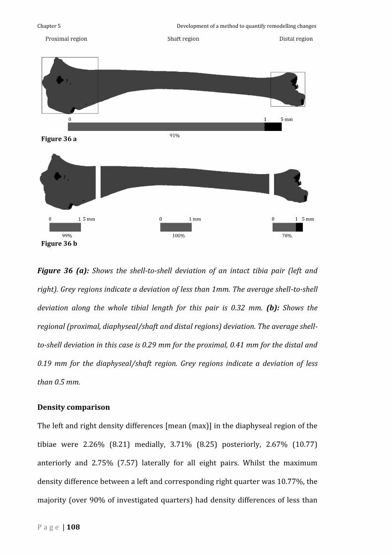
Chapter 5 Development of a method to quantify remodelling changes
P a g e | 108
Figure 36 (a): Shows the shell-to-shell deviation of an intact tibia pair (left and
right). Grey regions indicate a deviation of less than 1mm. The average shell-to-shell
deviation along the whole tibial length for this pair is 0.32 mm. (b): Shows the
regional (proximal, diaphyseal/shaft and distal regions) deviation. The average shell-
to-shell deviation in this case is 0.29 mm for the proximal, 0.41 mm for the distal and
0.19 mm for the diaphyseal/shaft region. Grey regions indicate a deviation of less
than 0.5 mm.
Density comparison
The left and right density differences [mean (max)] in the diaphyseal region of the
tibiae were 2.26% (8.21) medially, 3.71% (8.25) posteriorly, 2.67% (10.77)
anteriorly and 2.75% (7.57) laterally for all eight pairs. Whilst the maximum
density difference between a left and corresponding right quarter was 10.77%, the
majority (over 90% of investigated quarters) had density differences of less than
Figure 36 a
Figure 36 b

Chapter 5 Development of a method to quantify remodelling changes
P a g e | 109
5% (Figure 37). Figure 38 shows the average difference in density between intact
left and right tibia for one out of the eight tibia pairs.
Figure 37 Shows a density difference (%) histogram for intact left and right tibiae
pairs for the quarter volumes analysed (n =8).

Chapter 5 Development of a method to quantify remodelling changes
P a g e | 110
Figure 38 Shows the density difference (left vs. right) in percentage in each of the
four (medial, lateral, anterior and posterior) quarters for a sheep tibia

Chapter 5 Development of a method to quantify remodelling changes
P a g e | 111
5.3.2 Comparison of operated and intact contra-lateral tibia: Empty
defect (3 months post-operative)
The percentage density difference between an operated and intact pair for each of
the four quarters along the length of the diaphysis is shown in Figure 39. The
density differences were not uniformly distributed but rather in close proximity to
the segmental defect and the location of screw holes from the implant. The
maximum density differences (up to -50%) occurred in close proximity to the
segmental defect and in regions in close proximity to the screw holes (up to -30%).
The negative sign indicates a reduction in density value. However, in regions
farther from screw holes and the segmental defect, differences were less than ±5%
in all the four quarters analysed and in all 8 pairs. The peak density differences
adjacent to the segmental defect and the screw holes are shown in Figure 40.

Chapter 5 Development of a method to quantify remodelling changes
P a g e | 112
Figure 39 Shows the bone loss, as percentage change in density in each of the four
(medial, lateral, anterior and posterior) quarters for a sheep tibia with segmental
defect (SD) treated with a compression plate 3 months after surgery.

Chapter 5 Development of a method to quantify remodelling changes
P a g e | 113
Figure 40 Shows the peak density difference (%) in all quarters around the screw
holes and the segmental defect (SD) between the operated and intact contra-lateral
tibia at 3 months.

Chapter 5 Development of a method to quantify remodelling changes
P a g e | 114
Figure 41 Shows a density difference (%) histogram for intact left and right tibiae
pairs (dark grey) and operated and contra-lateral tibiae pairs (light grey) for the
quarter volumes analysed (n =8).
5.4 Discussion
The prime aim of this part was to determine whether the contra-lateral bone may
be used as a pre-operative control with respect to analyses of implant induced
bone remodelling in sheep. To address this question, firstly the extent of
anatomical similarity between left and right ovine tibias was investigated. As a
next step in this study, the magnitude of implant related bone-remodelling was
quantified to demonstrate that it is an order of magnitude greater than the
inherent contra-lateral differences and thus demonstrate the capability to use the
contra-lateral limb as a suitable control bone to determine patterns of bone
remodelling.
5.4.1 Intact left and right tibia comparison
The investigation of anatomical similarity began with an examination of the
geometric similarity. The geometric similarity between the pairs of intact bones
was not consistent across the three regions examined. While the diaphyseal and
proximal regions showed good similarity with average (n=8) differences less than

Chapter 5 Development of a method to quantify remodelling changes
P a g e | 115
0.5mm, the distal regions of the bone showed average differences of up to 1 mm.
The similarity for each of the different regions is partly explained by the alignment
procedure used. Because of the larger surface area of the proximal region, this
results in a larger number of points from this region that are used in the ICP
algorithm for alignment. Therefore, there is an alignment bias towards the
proximal end. Much of the disparity between the surfaces at the distal end can be
attributed to length differences between left and right tibia. Since the focus in this
study, was on the diaphyseal region of the tibia, in which 99 (92 – 100)% of the
region (measured points) had ≤1 mm surface deviation, the left and right tibial
surface can be considered to have good similarity in the diaphysis.
A density comparison of the paired tibiae was then conducted by dividing the
diaphyseal of the bone into quarters (Medial, Posterior, Anterior and Lateral), one
slice thick. The majority of these regions/quarters (90%) displayed density
differences of <5% (Figure 37). The remaining regions were divided between a 5-
10% difference range (<10% of regions) and a 10-15% range (<1% of regions).
The locations of the larger differences in density did not appear to show any
recurring pattern for the bone pairs compared.
Interestingly, the density analysis of the left and right bones found that the right
tibiae in all cases tended to have lower (1.78 ± 0.371%) density values than the left
tibiae (result is reported as average ± standard deviation, n=8). It is possible that
the lower bone density in the right tibia could be the result of a surgical procedure
(multi-fragmentary fracture and soft-tissue injury) that had been performed on the
right femur four weeks prior sacrifice. Though loading was not monitored in these
animals, it is plausible that the operated limbs were subjected to reduced weight
bearing. Thus, the density comparison of left and right tibia pairs incorporates

Chapter 5 Development of a method to quantify remodelling changes
P a g e | 116
potential density changes due to reduced weight bearing and subsequent
remodelling as well as the inherent bone differences. It is however unlikely that
the reduced weight bearing resulted in significant bone loss in the affected limb for
two reasons. Firstly, due to the relatively short time period of four weeks and
secondly, while the animals may have reduced weight bearing during normal gait
through limping, the bones were not completely unloaded as the animals
continued normal activities such as running, jumping, standing up and lying down,
all activities that can produce high loads on the tibia. Therefore, in a worst-case
where there may be some short-term effects of remodelling; the left and right
density differences are of the order of 5%.
The methods applied in this study are subject to limitations. The comparison of
bone density in corresponding quarters is subject to the accuracy of alignment of
left and right bones. Despite the very good alignment, evident in the low geometric
differences as described above, alignment between the two tibiae is not perfect
primarily due to differences in tibial length. Because the height of the quarters
compared (1 slice thickness = 0.67 mm) is less than the length differences (2-3
mm), the possibility exists that the compared quarters where slightly offset from
one another. Analysis of the variation in bone density between neighbouring slices
revealed average differences of 0.30 % ± 0.03 with a maximum difference from all
eight pairs of 1.9%. As the difference between adjacent quarters (approx 0.5%) is
an order of magnitude lower than the left and right differences (approx 5%), any
axial misalignment of one or two slices is unlikely to yield observable differences.
Figure 42 shows the percentage difference in density between adjacent slices of a
tibia for the length of the diaphysis.

Chapter 5 Development of a method to quantify remodelling changes
P a g e | 117
Figure 42 Shows the percentage density difference between adjacent CT slices of a
tibia in the medial quarter for one tibia pair. The lateral, anterior and posterior
quarters also showed density differences of < 2% between adjacent transverse slices
along the diaphyseal region of the tibia.
The method to align the tibia in the same orientation requires a transformation
followed by re-slicing. The re-slicing requires an interpolation of the DICOM data
to determine values for voxels in the re-sliced data that are located between the
original voxel positions. Since there is a high degree of similarity in density
between adjacent slices, the effects of this interpolation are expected to be
minimal.
Segmentation of the CT data to define the outer and inner surfaces of the cortex of
the tibia is subject to selection of an appropriate threshold value. Due to partial
volume effects (PVE) in CT datasets, which occur predominantly in border regions
where bone and soft tissue interface, a voxel spanning this region contains a
mixture of tissue types (Jiri, 2006) and the Hounsfield Unit (HU) stored in that
voxel is an average of the included tissues. This makes a clear determination of the
bone boundary difficult. While this artefact cannot be eliminated, by scanning both
paired tibiae in a single CT scan and then creating models from these scans with
the same intensity threshold, the two bones are treated equally and the effects of

Chapter 5 Development of a method to quantify remodelling changes
P a g e | 118
over or under-estimating the cortical boundary cancel out in both the geometric
and density comparison.
Statistical tests were not conducted in this study. Given a very small sample size
(n=8) and the complexity of design (8 tibia pairs with each tibia divided into 4
regions and data analysed at more than 200 slices for each pair); the appropriate
statistical test would be a multi level mixed model with random intercepts. When
the aforementioned statistical test was conducted, differences between left and
right tibiae were statistically significant (p<0.05). However, the mean estimated
difference was still < 3%. Although, the differences between left and right are
statistically significant (p<0.05), they are not scientifically significant when
considered that implant related bone remodelling changes (bone loss) are of the
order of (10-40%).
5.4.2 Operated and intact contra-lateral tibia comparison: Empty
Defect (defect was left untreated) (3 months post-operative)
Thus far this study has demonstrated that left and right tibial pairs have a high
degree of geometric similarity and comparable density distributions. For the
contra-lateral bone to be considered an appropriate control to quantify bone
remodelling, it must second be demonstrated that the density changes as a result
of remodelling are substantially greater than any left-right differences. A
comparison of operated (3 months post-surgery) and intact contra-lateral tibia
showed substantially larger density differences compared to those determined in
the left-right comparison.
As would be expected, operated (3 months after surgery) and intact contra-lateral
tibia comparison showed much larger differences in density than were seen in the
intact tibia pair comparison. The greatest density changes (bone loss) as a result of

Chapter 5 Development of a method to quantify remodelling changes
P a g e | 119
the osteotomy and plate fixation were seen in close proximity to the segmental
defect (10-50 %) and the screw holes (10-30%). The magnitude of the differences
observed where substantially larger than the differences between the left and right
matched pairs (5%). The location of the observed density differences between the
operated and the intact contra-lateral tibia were in regions influenced by the
defect and plate fixation. As the plate was affixed to the medial aspect of the tibia
the orientation of the screws was mostly in the medial-lateral plane. Accordingly,
the bone loss adjacent to the screw holes occurred predominantly in the medial
and lateral quarters.
The finding of bone loss around the screw holes is in agreement with qualitative
studies (Jiri, 2006; Sumitomo et al., 2008; Rathnayaka et al., 2010; Claes, 2011)
examining changes around fracture fixation implants, in which histological and
radiolographic techniques were used to assess bone density changes due to
remodelling. Although CT data has been previously used to quantify changes due to
remodelling (Engh et al., 1992), the comparison was performed using significantly
larger regions (i.e. Gruen zones; divided medially and laterally and each region
many slices thick) as compared to those in the present study (medial, lateral,
anterior, posterior, 1 slice thick). The techniques applied in this study have further
refined CT based evaluation methods by increasing their resolution which will be
useful in quantifying highly localized remodelling changes such as those occurring
as a result of fracture fixation. The methods developed here were capable to detect
bone remodelling changes associated with fracture fixation.
5.5 Conclusion
In summary, left and right ovine tibiae were found to have a high degree of
geometric similarity with differences of less than 1.0 mm in surface deviation and
Chapter 5 Development of a method to quantify remodelling changes
P a g e | 120
density difference of less than 5% in the diaphyseal region (N.B. The similarity
between an ovine tibia and its contra-lateral pair is been accepted to be published
in Medical Engineering and Physics Journal (Krishnakanth et al., 2011) (refer to
Appendix D) The density differences occurring as a result of implant related bone
remodelling (10-40%) were well above the observed contra-lateral differences.
Although recent studies in small animal models have produced conflicting results
as to whether remodelling effects are confined to the bone subjected to external
loading or whether the contra-lateral is affected through systemic neuronal
pathway (Sample et al., 2008; Sugiyama et al., 2010), in this study localised implant
related remodelling produced substantial differences with respect to the contra-
lateral bone.
Hence, it can be concluded that for the purposes of implant related bone
remodelling investigations in sheep, the intact contra-lateral tibia may be
considered an alternative to a pre-operative control, provided that the changes in
density due to remodelling yield differences greater than 5% and including a
margin of safety, only changes greater than 10% should be considered as a result
of remodelling. Although limited to the diaphyseal region and only to the cortical
bone, this method may be used to quantify the pattern of bone remodelling in
experimental situations. The quantified patterns of bone remodelling may then
serve to validate the predictions of numerical algorithms simulating bone
remodelling.

P a g e | 121
6 Validation of bone remodelling quantification
method
In this chapter, the bone remodelling quantification method developed in Chapter
5 is further validated by comparing changes between an intact and an
osteotomised contra-lateral tibia stabilised with three different type of therapeutic
approach (Empty defect; defects left untreated, defects reconstructed with a
cylindrical mPCL-TCP (polycaprolactone tricalcium) scaffold with or without
rhBMP-7 (Bone Mineral Protein) and at different time points after the surgery (3
and 12 months). The above three treatment groups were chosen because; the
differences in healing pattern between these groups due to differences in loading
were expected to ultimately result in differences in remodelling changes.

Chapter 6 Validation of bone remodelling quantification method
P a g e | 122
6.1 Introduction
In chapter 5 density changes due to implant related remodelling was quantified
and the results demonstrated that the implant related remodelling changes in
terms of bone loss are well above the inherent contra-lateral differences. In this
Chapter, further validation of the developed CT based remodelling quantification
method was performed by comparing remodelling changes between three
different therapeutic approaches and at two different post-operative time points
after surgery.
CT data of ovine tibias stabilised with three different therapeutic approaches;
Empty defect (defects left un-treated), defects reconstructed with mPCL-TCP
(polycaprolactone tricalcium phosphate) scaffold and mPCL-TCP scaffold coated
with rhBMP-7 (Bone Mineral Protein) at 3 and 12 months after surgery obtained
from a parallel study was used for investigation.
It is believed that remodelling changes are influenced by the type of fixation device
or the treatment method adopted to stabilise fractures owing to differences in the
loading environment created by the implant or the treatment approach adopted.
Since bone adapts to changes in loading environment through the process of
remodelling, it was expected that there would be differences in remodelling from
one group to the other. As mentioned earlier, CT data of ovine tibiae were obtained
from a parallel study within the research group which was designed to investigate
the effect of these three different treatment approaches on the mechanical
properties of the newly formed bone in the defect region (Reichert et al., 2010).
Here, it was demonstrated that there were differences in the volume of newly
formed bone in the defect area for the groups investigated (Figure 43). Due to this,
we expect differences in loading environment of the healing bone and hence

Chapter 6 Validation of bone remodeling quantification method
P a g e | 123
remodelling differences between the groups. Figure 44 shows the path of load
transmission for the groups where defect was left untreated (empty defect) and
defect reconstructed with a mPCL-TCP scaffold with and without rhBMP-7.
Figure 43 Representative 3D CT reconstructions of critical segment bone defects,
which were left untreated (A), reconstructed with a mPCL-TCP scaffold (B) and a
mPCL-TCP scaffold combined with rhBMP-7 (C).(modified from 17).
Additionally, given sufficient time for remodelling to occur, data obtained at
different time points (3 and 12 months after surgery) are also expected to show
differences in remodelling.
17 (Reichert et al., 2010)

Chapter 6 Validation of bone remodeling quantification method
P a g e | 124
Figure 44 Demonstrates the differences in load transmission path between empty
defect and groups with PCL-TCP scaffold.
In order to understand the remodelling pattern induced by any particular type of
fixator, changes due to remodelling need to be quantified. Therefore, the purpose
of this study was to further investigate the pattern of remodelling changes
observed not only between different treatment groups but also at different
time points. The knowledge thus gained will aid our understanding of the factors
driving the implant related remodelling changes.
In this study contra-lateral limb is used as a pre-operative control. The use of
contra-lateral limb to enable changes due to remodelling to be discerned is verified
in Chapter 5 (refer to 5.1.3 Use of contra-lateral ovine tibia as a pre-operative
control in bone remodelling analysis) of this thesis.
Chapter 6 Validation of bone remodeling quantification method
P a g e | 125
6.2 Materials and methods
Specimens were obtained from a parallel study. CT scans of forty pairs of tibia from
three different therapeutic approaches at 3 and 12 months after surgery were used
to determine changes due to remodelling. In all the three groups, sheep underwent
a mid-diaphyseal osteotomy of the right tibia to create a 3 cm defect which was
stabilized with a compression plate (7-hole DCP (Dynamic Compression Plate),
Synthes AG, Switzerland). In the first group the defects were left un-treated and
the defect was reconstructed with a cylindrical mPCL-TCP scaffold in the second
group. In the third group the scaffold in the defect region was coated with rhBMP-
7. CT data for empty defect group was available only for the 3 months post-
operative period.
The procedure described in chapter 5 (refer to Chapter 5: Volume comparison)
was used to compare density changes due to remodelling between different groups
(operated and intact contra-lateral tibia pairs) in this part of the thesis and hence
only briefly explained in the following paragraph.
As noted above, animals were sacrificed 3 (n=8) and 12 (n=8) months after
surgery and the fractured and intact contra-lateral tibia after removal of implant
were CT scanned together with a bone phantom (EFP) for comparison. A single
intensity threshold (200 HU) was used to create surface models of the tibia from
the CT data. The surfaces of the paired tibiae were then positioned in the same
orientation thus aligning the original CT data for matched tibia pairs before any
comparison. The density differences were determined between the operated and
the intact contra-lateral bone by dividing the CT data in the diaphyseal region into
discrete volumes, defined by a quarter of a transverse CT slice. As the bones were
scanned together with a bone phantom (EFP), a relationship between the HU

Chapter 6 Validation of bone remodeling quantification method
P a g e | 126
values and apparent density of Hydroxyapatite in each of the phantom’s chambers
was established allowing conversion of HU values to bone mineral density (BMD).
The averaged density difference between corresponding volumes was computed.
Localized changes in BMD in regions in close proximity to the screw holes and the
segmental defect (SD) were determined by averaging the percentage density
differences over adjacent slices. Only BMD values corresponding to cortical bone,
with an intensity value greater than 600 HU (Rathnayaka et al., 2010) were
considered in the analysis.
6.3 Results
6.3.1 Density changes within the cortical region
Reductions in average density in the cortical bone of up to 50% were seen at 3 and
up to 60% at 12 months after surgery in regions in close proximity to the
segmental defect in the three groups analysed. The peak differences in density in
regions in close proximity to screw holes and the segmental defect (SD) between
the three treatment groups at 3 and 12 months are as shown in Figure 45 and
Figure 46 respectively for medial and lateral regions.
Figure 45 a

Chapter 6 Validation of bone remodeling quantification method
P a g e | 127
Figure 45 Shows the change in density (%) at 3 months for the medial (a) and
lateral (b) aspects of the tibia for the empty defect (Black), scaffold (Light Grey) and
scaffold with BMP (Dark Grey) groups (mean ± standard deviation). SD=Segmental
Defect.
Figure 45 b
Figure 46 a

Chapter 6 Validation of bone remodeling quantification method
P a g e | 128
Figure 46 Shows the change in density (%) at 12 months for the medial (a) and
lateral (b) aspects of the tibia for the scaffold (Light Grey) and scaffold with BMP
(Dark Grey) groups (mean ± standard deviation). SD=Segmental Defect.
Density changes at 3 months
The pattern of reduction in average density in the cortical bone was similar in all
three treatment groups and across all four regions analysed with reductions of up
to 50% in regions in close proximity to the segmental defect and the regions
adjacent to it. Also, greater density reductions in density (bone loss) were
observed in regions in close proximity to screw holes and SD as opposed to regions
further from it. Furthermore, the medial and lateral regions showed greater
reductions (bone loss) of up to 50% in close proximity to screw holes while
differences in anterior and posterior regions were up to 20%. However, the empty
defect group showed lesser reductions in density of up to 30% (segmental defect
and the adjacent regions) than the groups with scaffold and scaffold with BMP
where differences were up to 50%.
Figure 46 b

Chapter 6 Validation of bone remodeling quantification method
P a g e | 129
Density changes at 12 months
Similar reductions (bone loss) in density was observed at 12 months where more
pronounced changes (up to 60%) was observed for lateral and medial regions in
both PCL TCP scaffold and PCL TCP scaffold coated with BMP groups, while
reductions of up to 30% was observed for anterior and posterior regions. However
the magnitude of differences in density in close proximity to the segmental defect
and the adjacent regions was greater (60%) than that observed in close proximity
to screw holes (50%) (Figure 46).
6.4 Discussion
6.4.1 Density changes within the cortical region
In this study the magnitude of implant related bone remodelling was quantified for
different treatment groups and at different time points to investigate possible
differences between the groups owing to differences in loading patterns and time
periods. As to be expected, the greatest density reductions occurred in close
proximity to the segmental defect and the screw holes, in particular the innermost
screws. In addition, there was a pattern of observed reductions in density which
was similar between all three treatment groups and at both time points i.e., the
reductions in density was more pronounced in the plane of fixation (medial and
lateral planes) and in regions influenced by the fixator (screw holes) and the defect
itself than the anterior and posterior planes (density differences < 10%).
Density changes at 3 months
The pattern of bone remodelling in the empty defect group was similar to the
group treated additionally with a rigid mPCL-TCP scaffold and PCL-TCP scaffold
coated with rhBMP-7. Greater reductions in density in regions adjacent to defect
Chapter 6 Validation of bone remodeling quantification method
P a g e | 130
were reasoned to be the result of stress shielding effect (refer to Stress shielding;
2.4.2 Fixation stability and remodelling) in the presence of an implant. Since
most of the load gets transferred through the fixator, the bone predominantly in
the defect region is unloaded during initial stages of healing (before callus
formation) and thus, this unloading leads to bone loss or atrophy due to functional
adaptation of bone to changes in mechanical loading.
Although the reductions in density between operated and intact contra-lateral
tibial pairs were more in the regions adjacent to screw holes and the segmental
defect than the regions farther from the fixator, it was expected that the magnitude
of changes due to remodelling varies between different treatment groups. Less
bone loss was expected to occur in the groups reconstructed with scaffold than the
empty defect group, in particular, in the defect region, due to the continuous path
of load transmission maintained by the scaffold (Figure 44). However, contrary to
our expectation, bone loss tended to be greater in the groups reconstructed with a
scaffold relative to the empty defect group. It was reasoned that greater bone loss
observed in regions around the defect in the scaffold groups could be the result of
biological integration of the scaffold onto the bone material. Introduction of
scaffold in the defect region could have initiated such bone loss in defect region
during the process of integration of scaffold material on to already denser cortical
bone.
In addition, there was no significant difference in density changes between the
scaffold and scaffold coated with rhBMP-7 groups. Also, reductions in density
observed in regions in close proximity to screw holes farther from the segmental
defect were less (15%) than that observed in regions in close proximity to

Chapter 6 Validation of bone remodeling quantification method
P a g e | 131
segmental defect (up to 45%) and such bone loss could be the result of implant
insertion process (drilling of screw holes).
Density changes at 12 months
Contrary to our expectation the magnitude of density differences (bone loss)
observed at 12 months was greater than that observed at 3 months (remodelling
or bone formation over time). However, reductions in density observed in regions
in close proximity to screw holes farther from the segmental defect at 12 months
was found to be of the around the same magnitude as observed at 3 months and
was seen across both treatment groups (scaffold and scaffold with BMP) and for all
four regions analysed. In such a case, the changes due to remodelling could be
related to trauma and the type of treatment rather than changes in loading pattern
in the presence of an implant. However, it was evident from the results that there
was a considerable increase in the percentage of reduction in density in the
regions in close proximity to the defect at 12 months than at 3 months. It is
possible that such a reduction could be the combined effect of integration of the
scaffold and BMP material onto the regions adjacent to the segmental defect as
well as stress protection. This combined effect was also seen to be spilled over to
regions of screw holes adjacent to the defect.
This study is subject to a few limitations. From the results of this analysis we
recognise that the treatment groups (empty defect, PCL-TCP scaffold and PCL-TCP
scaffold with BMP) chosen for the analysis might not be suitable in discerning
changes in remodelling due to changes in loading pattern alone. However, with
intent to reduce the number of animals used for experiments, we obtained
specimens (CT data) from a previous study which was readily and timely available.
Furthermore, owing to differences in loading patterns between the treatment
Chapter 6 Validation of bone remodeling quantification method
P a g e | 132
groups, we believed the specimens would be adequate to demonstrate changes in
remodelling pattern due to changes in loading conditions between them.
6.5 Conclusion
As there was no considerable difference in density changes at different time points,
and that the data for the groups where the defect was left untreated was available
only at 3 months, the bone remodelling changes observed might be related to both
the initial trauma or the type of treatment (scaffold and/scaffold coated with BMP)
as well as adaptation to the changed loading condition. Also, contrary to the belief
that remodelling is stimulated by changes in loading conditions, empty defect
treatment group showed less bone loss than the other two groups where scaffold
was introduced at the segmental defect region. It is believed that data from
different treatment groups or from longer post-operative time periods might result
in significant remodelling changes between them, thus providing further insight in
to the factors driving the remodelling changes (such as changes in loading
patterns).
In conclusion, although the groups investigated might not be suitable to produce
significant differences in bone remodelling in response to changes in loading
conditions, the presented method to quantify remodelling across the entire
diaphyseal region (cortical bone) of the bone enabled changes around localised
features, such as plane of fixation, screw holes and segmental defect to be
discerned. Hence, the developed bone remodelling quantification method can be
considered suitable in quantifying changes due to implant related remodelling.

P a g e | 133
7 Overall discussion and conclusion
This project focussed on characterising fixation stiffness of internal plate fixation
devices. Furthermore, a CT based implant related remodelling quantification
method was also developed. Knowledge gained in this project will be useful in
configuration and design of internal plate fixation devices which not only promotes
healing but also prevents undesirable bone loss through remodelling. This Chapter
discusses the main findings of this PhD project along with a mention of future
directions.

Chapter 7 Overall discussion and conclusion
P a g e | 134
7.1 Discussion
Section 1: Fixation stability and healing
The objective of the first section of this project was to characterise the stiffness
of an internal plate fracture fixation device. In-silico or computer methods were
used to evaluate the different fixation stiffness determination methods and an
appropriate method to determine the stiffness characteristics of an internal plate
fixation device using Finite Element Analysis (FEA) was defined. The developed
method was then used in the characterisation of internal plate fixation stiffness
where the influence of modifications to fixator configurations on implant stability
was investigated.
The mechanical conditions in the fracture gap are thought to play a decisive role
not only in the overall healing outcomes of the bone but also in the remodelling of
the adjacent bone fragments. In fact with a good blood supply, the course of
fracture healing has been reported to be primarily influenced by the inter-
fragmentary motion, which in turn is determined by the applied load and the
stability of fixation device. Such mechanical conditions which each fixator creates
however are poorly understood. Experimental tests in animal models have studied
the effects of various fixators on healing and remodelling. The outputs of these
tests however – histology, mechanical testing etc, provide only a brief summary of
the results rather than a detailed understanding of the mechanism.
Finite Element (FE) modelling of the bone-fixator construct can be used to
simulate the conditions in the fracture gap. If these conditions are known then
their resultant effects on healing and remodelling can be studied and adaptations
made to the designs to improve outcomes.

Chapter 7 Overall discussion and conclusion
P a g e | 135
Comparison of boundary conditions demonstrated that applying loads closer to the
Fracture Gap (FG) reduces the unwanted indirect moments. A convenient way to
do so in FE is by using MPC (Multi Point Constraint) boundary conditions. The
developed in-silico method (MPC boundary condition and individual stiffness
calculation methods) of fixation stiffness determination provides a convenient way
to investigate the influence of modifications to fixator configurations on implant
stability.
Previous studies have evaluated the 3D stiffness (stiffness in 6 directions) of
external fixators and tibial nail in-vitro (Kassi et al., 2001; Epari et al., 2007; Augat
et al., 2008). This study represents one of the first attempts to characterise 3D
internal fixation stiffness (Locking plate) using computer model/FE. Although
during the past years several fracture fixation stiffness determination methods
have been reported in literature, there exists no universal stiffness determination
method which can be adopted owing to differences in functioning of fixation
devices. The deformation behaviour of all fracture fixation devices is not similar.
For example, unlike external ring fixators, the primary deformation mode of
internal plate fixators under axial load is more akin to bending. Due to the short
bending length of the screws, the whole construct results in bending, while the
longer bending length of the screws in external fixation devices allows the
construct to undergo more axial movement and less bending under axial loads. The
present study offers comparison between different methods and investigates the
influence of these methods on the implant stability. The purpose of this study was
not to show superiority of any particular method but rather to demonstrate
appropriateness of these methods to characterise internal plate fixator stiffness.

Chapter 7 Overall discussion and conclusion
P a g e | 136
The investigations showed that factors such as simulated boundary conditions, the
point of load application and the manner in which fixation stiffness is calculated
ultimately influences the value of fixation stiffness determined and that some
methods may not be suitable in characterisation of fixation stiffness of some of the
fracture fixation devices.
This study investigated two methods of applying loads (axial compression and
rotation) to the proximal part of the bone-fixator construct; Kassi (confined lateral
and rotational movements of the proximal fragment) and Augat (unconfined
lateral and rotational movements of the proximal fragment). For the case of
internal plate fracture fixation devices, due to the shorter length of the screws and
closer placement of the plate to the bone’s surface, the construct is more akin to
bending. By confining the movement of the proximal fragment, the main mode of
movement (bending in medial-lateral direction) associated with unilateral internal
fixation devices is restricted and hence makes the system overly stiff. Therefore,
such a boundary condition although suitable for external fixators may not be
appropriate to simulate the load-displacement behaviour of internal fracture
fixation devices. Moreover, confined compression or rotation does not represent
in-vivo deformation behaviour since in physiology the bone-implant system is not
restricted of lateral or rotational movements of the proximal fragment.
Likewise, investigation of shear fixation stiffness when the shear load was applied
to the top end of the proximal fragment (Kassi) suggested that it produces more
bending of the construct at the fracture gap due to the relative position of the
fixator in relation to the long axis of the bone. This undesirable effect due to
excessive bending at the fracture site was reduced when loads were applied close
to the fracture gap.

Chapter 7 Overall discussion and conclusion
P a g e | 137
Moreover, the study highlights the problems associated with the use of stiffness
matrix for calculation of fixation stiffness. The neutral axis of composite plate-bone
structures is located very close to the external surface of the bone or even inside
the plate because the elastic modulus of the plate (200 GPa) is much greater than
that of the bone (16 GPa) as well as due to discontinuity in bone (segmental
defect). Due to this, the system produces asymmetric deformation behaviour due
to eccentric loading conditions. Example, shear in anterior-posterior direction and
axial torsion resulted in similar IFM’s. Shear load in anterior-posterior direction
not only resulted in shear IFM (Inter-fragmentary movement), but also resulted in
a torsional moment about the fracture gap. Due to the shift of neutral axis, it is
quite complex to determine the position of the neutral axis of the combined
structure (osteotomised tibia stabilised with internal plate fixator) which will help
in realising this rotational moment. Since the stiffness matrix did not account for
the indirect axial rotation moment caused by this shear force about the fracture
gap, it resulted in errors in stiffness calculation and very high stiffness values.
Therefore, the suggestion to use the individual stiffness calculation method for
internal fixation stiffness calculation was made.
If the aim of any study is to compare fixation stiffness for different fixator
configurations in FE where relative and not absolute values are important, this
study suggests the use of MPC boundary condition and individual stiffness
calculation method as it reduces the unwanted effect due to indirect and
unaccountable out of plane forces which are hard to determine.
Primarily, this project aimed at investigating the influence of modifications to
fixator configurations on implant stability by making alterations to fixator
configurations such as material property, fixator axis inclination with respect to

Chapter 7 Overall discussion and conclusion
P a g e | 138
the long axis of bone, offset distance between fixator and bone surface, distance
between inner most screws (Working Length), position, spacing and number of
screws and use of FCL (Far Cortical Locking) screws.
Investigation of the influence of modification to fixator configurations on implant
stability suggests that there is more than one way to alter fixation stiffness to meet
better healing requirements. However, the choice also depends on type, location
and severity of the fracture among other factors.
The hypothesis that the internal fixation devices (locked plates) are invariably stiff
was supported by the observed axial IFM which was <0.14 mm at the near and
<0.34 mm at the far cortex for the standard (three screws on either side of the
fracture gap leaving the middle three screws holes empty) fixator configuration.
Shear IFM were also invariably small (<0.05 mm) for the fixator configurations
investigated making the fixation device stiffer against shear loading. The current
state of the art in creating models of bone-fixator systems is to model the
interfaces (bone-screw and screw-plate) as fixed. It is believed that the FE results
will be overestimated due to such perfectly modelled interface and FE model
comparison conducted has shown that the results from FEA are over estimated up
to a maximum of 70% (refer to Appendix C) when compared with results from in-
vitro. Hence, even with 70% over estimation, for the fixator configurations
investigated in this study, it is believed that the axial and shear IFM are still very
small and hence it can be concluded that these devices are inherently stiff fixation
devices.
The motivation of this study was that, fixators that allow moderate axial IFM but
provide higher resistance to shear and torsional movements to be better for

Chapter 7 Overall discussion and conclusion
P a g e | 139
successful and timely healing. Although the standard fixator configuration
(0XXX0XXX0) was invariably stiffer than the published stiffness values for external
fixators in-vitro (Epari et al., 2007)so as to allow moderate axial IFM, this study has
shown that by making certain modifications to fixator configurations in terms of
fixator material (Ti), offset distance (3 mm), working length (three screw hole
width) and introduction of Far Cortical Locking (FCL) screws the axial micro
motion can be increased to stimulate callus formation for healing. However, some
of these modifications resulted in reducing shear and torsional stiffness attributes
when compared to standard configuration (0XXX0XXX0), which should be
maintained in order to stimulate callus formation for timely healing. Since, shear
IFM for all the fixator configurations investigated was less than 0.1 mm, it can be
considered that the internal fixation devices are stiff against shear loading even
with the above modifications to configurations.
Of the suggested modifications to increase axial IFM, the use of FCL screws was one
of the options to stimulate callus formation towards better healing outcome.
However, the use of FCL screws in clinics may pose certain complications which
have not yet been investigated. Firstly, these FCL screws lock into the plate and
onto the far cortex of the diaphysis. This allows for elastic flexion of the screw
under the application of loads at the near cortex thus enabling parallel IFM. All
loads are directly transferred from the plate to the far cortex through flexible
shafts (screw shaft). While this may permit IFM stimulatory to healing, particularly
at the near cortex, the effect the flexion of FCL screws has against bone’s surface in
areas particularly adjacent to screw holes is not yet been investigated. It is
expected that such an arrangement might result in bone resorption in regions
around screw holes at the near cortex. Further investigations are required to
determine the effect of FCL screws on fracture healing and remodelling.

Chapter 7 Overall discussion and conclusion
P a g e | 140
There are a number of issues that were not addressed in the current study as the
primary focus of this study was characterisation of fixation stiffness and hence the
study did not include investigations related to implant survival. In future studies
addressing implant survival, it would be interesting to investigate the stresses
experienced by the construct as they are particularly important in deciding the life
of the implant, multifaceted and physiological loading conditions and fatigue tests.
In addition, results of this study are limited to investigation of single mid-
diaphyseal osteotomy. Behaviour of the bone-implant system may be different for
fractures with large fracture gaps and multiple fractures.
The current state of the art in creating models of bone –fixator constructs is to
model the interfaces as being fixed. Little mention is actually made in the literature
as to the appropriateness of this technique This assumption (fixator-bone
interfaces modelled as fixed in all DoFs) made during the creation of finite element
model about the screw-bone and plate-screw interface) might over estimate the
fixation stiffness. However, the FE model used in this study is been compared
against results from in-vitro tests Since the investigation of the influence of
modifications to fixator configuration on its stiffness is based on relative
comparison, absolute values are not important. Therefore, the simulated perfect
screw-bone or plate-screw interface was assumed to be uncritical
It should be pointed out that studies such as this were not intended to represent
clinical situation and therefore cannot accurately predict complex in-vivo
behaviour. However, they do provide useful information to the surgeon on the
influence of fixator configuration on implant stability. At present due to the
minimal invasive surgical techniques, certain factors that affect fixation stiffness
are sometimes beyond surgeon’s control. Example, the limited visibility of the

Chapter 7 Overall discussion and conclusion
P a g e | 141
fracture site and sliding of the plate from a cut made at a distance from the fracture
zone may result in some amount of inclination between the plate and bone axis.
The parameter investigation suggests that such slight inclination of the plate axis
with the bone does not affect axial compressional stiffness. Additionally, since
working length was shown to be the greatest determinant of fixation stiffness and
the spacing and position of screws had only minor influence, it gives the surgeon a
wide range of options (screw configuration) especially in situations where certain
screw spacing cannot be avoided.
The in-silico methods developed in this project enabled investigation of
parameters that influence fixation stiffness. The parameter analysis conducted in
this section has strengthened our knowledge about the influence of fixator
configuration on its stiffness characteristics and may further be used to suggest
modifications to screw configuration which results in optimal stiffness conditions.
The knowledge gained here will aid in the configuration of fixation stiffness for
optimal healing conditions via in-vitro tests. As mentioned earlier, results from this
study demands further research investigating the influence of FCL screws on
adverse effects of bone remodelling of the surrounding bone fragments.
In conclusion, the investigation of fixator configuration on implant stability using
developed in-silico methods is an effective way to investigate the influence of
fixator configurations on implant stability. However configuration of optimal
fixator configurations of final constructs for better healing should include in-vitro
tests (FE results are over estimated due to perfectly modelled interfaces). Hence,
further in-vitro studies are required in the assessment of stiffness of final
constructs and the results from this parametric evaluation may only be used as a
guideline for implant design.

Chapter 7 Overall discussion and conclusion
P a g e | 142
Section 2: Fixation stability and remodelling
In the second section of this project, a CT based bone remodelling
quantification technique was developed. In the process of the development of
this quantification method, the use of contra-lateral ovine tibia as a suitable pre-
operative control with respect to the analysis of changes due to implant induced
bone remodelling was validated. The developed remodelling quantification
method was then used to quantify implant related remodelling changes between
different treatment groups (Empty defect, PCL-TCP scaffold and PCL-TCP scaffold
with BMP) and at two different time periods (at 3 and 12 months post operative).
The presented CT based bone remodelling quantification method was able to
identify changes due to remodelling around the fixator, especially in the plane of
fixation and in regions near screw holes and segmental defects.
Previously, studies have assumed the use of contra-lateral limb to serve as a
suitable control in remodelling analysis. In this study, for the first time, the use of
contra-lateral ovine tibia as a pre-operative control in analysis of changes due to
remodelling is validated. Since the differences in geometry was < 3% and density
differences were < 5% between intact left and right tibiae and differences between
operated and intact were of the order of 40% (bone loss) in regions of screw holes
and segmental defect, it was concluded that contra-lateral bone can be used as a
suitable pre-operative control. In this study, all the intact tibiae were extracted
from animals which underwent a previous surgery on their right femur. It was
expected that the differences between left and right would also include differences
due to reduced weight bearing on the right limb which was justified by higher
density values found for left tibiae in all 8 pairs analysed. Hence, this validation
study accounts for the reduced weight bearing of the operated limb.

Chapter 7 Overall discussion and conclusion
P a g e | 143
Quantification of implant related remodelling changes between different
therapeutic approaches and at different post-operative time periods showed that
bone atrophy especially in the defect region is unavoidable. Interestingly, the
results showed that the magnitude of bone loss in regions in close proximity to
screw holes did not worsen at 12 months as compared to data at 3 months and
such bone loss (15%) could be more related to implant insertion procedure
(drilling of screw holes) rather than changes due to loading conditions. In the
regions adjacent to defect and inner most screws, the bone loss data (50%) was
due to combined effect of stress protection and biologic integration of scaffold
material on to the surrounding cortical bone and such an effect was found to
increase at 12 month post-operative. It was expected that at 12 months, there
would be less bone loss than at 3 months due to changes in loading (more load is
expected to pass through the callus at 12 months thus resulting in new bone
formation around the defect). Hence, the question is, should the implant be
removed since it is causing bone loss due to stress protection? Investigation of
implant related bone remodelling changes for longer post-operative periods may
be necessary before making a decision on implant removal.
The treatment groups chosen for comparison was readily and timely available
from a parallel study and not handpicked to demonstrate distinguishing changes in
remodelling patterns between the groups. Changes in loading pattern between the
different treatment groups, was believed to result in differences in the magnitude
of changes due to remodelling between these groups. However, realisation of
changes in remodelling due to difference in loading patterns as expected between
different treatment groups and at different time points was not identifiable using
the developed quantification method. Therefore, it is assumed that there may be
other factors driving the remodelling process apart from the changes in loading

Chapter 7 Overall discussion and conclusion
P a g e | 144
patterns and data from longer time periods (> 12 months) might be required to
discern changes in remodelling between different treatment groups. Also, it is
expected that comparison of density data when performed on volumes smaller
than a quarter of a transverse slice may help identify the localised changes in
remodelling (smaller regions may aid in better identification of localised
remodelling changes which otherwise might be compromised due to averaging of
density values when larger volumes are analysed) between different treatment
groups (changes in remodelling due to change in loading pattern) to be discerned
and can be a focus of future studies.
The study is subject to a few limitations. Post-processing of CT data (segmentation
and transformation) led to changes in original CT data by around 2%. However,
such alterations are un-avoidable. Hence we concluded that density changes >10%
(twice the density difference observed between left and right intact tibiae) can be
considered as changes due to implant related remodelling thereby accounting for
post-processing errors.
The developed CT based bone remodelling quantification technique (refer to
Chapter 5; Volume comparison) has enabled quantification of changes due to
implant induced remodelling. The remodelling quantification tool can now be used
to quantify changes due to implant related remodelling which are more localised.
This will aid our understanding of how much remodelling occurs around implants
and will help clinicians decide whether the amount of remodelling which occurs
around orthopaedic implants; internal fixation plates in this case, is a threat to
implant survival? Furthermore, this quantification method can also be used to
validate existing bone remodelling simulation algorithms which can predict
implant related remodelling changes.

Chapter 7 Overall discussion and conclusion
P a g e | 145
Further improvements can be made to the existing quantification method such that
comparison of smaller volumes (smaller than quarter of a transverse slice) is
possible which may enable identification of highly localised remodelling changes
between different treatment groups.
The introduction of dual energy CT scanners (Gemini PET-CT scanner; Philips
Medical Systems, Discovery CT 750 HD; GE Healthcare) is been effective in
reducing metal artefacts caused by orthopaedic implants due to better image
quality. However, it is still to be investigated whether these scanners may make
possible the possibility of performing quantifications in human bones with
implants.
7.2 Conclusion
In conclusion, this study has shown that it is possible to achieve moderate axial
stiffness so as to promote better healing by making certain modifications to fixator
configurations; however some of these modifications could also result in lowering
shear and torsional stiffness which should be maintained in order to promote
better healing outcome. Additionally, internal plate fixation devices were found to
be comparatively stiff fixation devices.
In this study it was shown that the contra-lateral limb can be considered to
represent the pre-operative state of the operated ovine tibia for remodelling
analyses. In addition, the fact that we were able to quantify highly localised
remodelling changes in the plane of fixation and in regions around fixator screws
illustrates the sensitivity of this CT based bone remodelling quantification method.
This PhD project can be furthered by creating an FE model for one of the treatment
groups for which changes due to implant related remodelling has been already

Chapter 7 Overall discussion and conclusion
P a g e | 146
quantified in Section 2 of this project (e.g. Empty defect, PCL-TCP scaffold or PCL-
TCP scaffold with BMP). Then, conducting subsequent FE simulations using the
developed in-silico methods (Section 1) will help establish a relationship between
fixation stiffness and/or initial IFM and the amount of remodelling changes for the
fixator chosen. It is believed that such an analysis will aid in the configuration of
internal plate fixator not only for better healing but also for better remodelling
(reduction in bone atrophy).
Overall, this project has delivered and aided our understanding of the influence of
fixator configurations (internal fixation plates) on its stiffness characteristics
which, in turn influences the fracture healing process and the remodelling of the
adjacent bone fragments. Knowledge gained in this study will be useful to further
our understanding in the configuration and design of internal fixation devices
which not only promotes timely healing but also prevents undesirable bone loss.

Appendix A
P a g e | 147
Appendix A: Determination of IFM (Inter-Fragmentary
Movement)
The translational Inter-fragmentary movements were determined from the
displacement of a node positioned at the centre of the fracture gap attached to the
upper fragment relative to a coincident node attached to the lower fragment as
shown in Figure 47.
Figure 47 Illustrates calculation of translational inter-fragmentary movements.
The rotational inter-fragmentary movements were calculated using matrix algebra
which is explained in the following paragraphs.
Proximal fragment
Distal fragment

Appendix A
P a g e | 148
Calculation of rotational inter-fragmentary movements
Defining LCS (Local Coordinate System): Firstly a local coordinate system (LCS)
was set up for each bone fragment. A LCS is a reference system that is fixed within
a body or a segment and moves along with it. The global coordinate system (GCS)
also called as the reference coordinate system is the fixed coordinate system from
which all positions are ultimately derived. It is a right handed orthogonal
coordinate system. In this analysis, GCS was defined by X axis pointing posterior-
anterior direction, Y axis medial-lateral, and Z axis pointing distal-proximal
direction as shown in Figure 48. The unit vectors for the GCS are→
i ,→
j and→
k
respectively. The unit vectors are the vectors of unit length along each axis
representing the coordinate system and were represented by,→
i ,→
j and→
k along X, Y,
Z axis respectively. The LCS was oriented such that x axis of the LCS points
posterior-anterially, y axis medial-laterally and z axis distal-proximally. The
orientation of the LCS with respect to GCS defines the orientation of the body in 3D
space and it changes as the body moves in space.
Three non-collinear points/nodes were chosen on each bone fragment and the LCS
was set up using equations from matrix algebra which are listed below. The
selection of three points is as shown in Figure 48. First subtracting the position of
point UA from UB, and by dividing by the norm of the vector created by (UB-UA),
gave rise to a unit vector which has its origin at UA and pointing towards UB, i.e., in
→
j direction, lateral-medial axis of the segment. Now the →
i axis, the posterior-
anterior axis was determined in two steps. Again, subtracting (UB-UA) created a
vector originating from UA and pointing towards UB. Next, subtracting (UC-UA)
gave a vector originating from UA and pointing towards UC. By performing a cross
product and dividing by the norm as shown in equation, the result was a unit

Appendix A
P a g e | 149
vector, →
i in the posterior-anterior direction. The third axis of the LCS,→
k , the
distal-proximal axis, was determined by the cross product of the two unit
vectors, →
i ×.→
j The order of vectors in the cross product was determined by the
right hand rule.
Figure 48 Illustration of calculation procedure for unit vectors that forms the LCS
and the Rotation Transformation Matrix (RTM). (ULCSO = Upper Local Coordinate
System at time zero).
At first, ULCS (Upper Local Coordinate System), LLCS (Lower Local Coordinate
System) were defined in a matrix form, in which the rows represent the 3D
coordinates of,→
i ,→
j and →
k unit vectors of the LCS of the two bone fragments.

Appendix A
P a g e | 150
ULCS =
kkk
jjj
iii
zyx
zyx
zyx
'''
'''
'''
, LLCS =
kkk
jjj
iii
zyx
zyx
zyx
''''''
''''''
''''''
Calculation of rotation matrix
The RTM (Rotation Transformation Matrix) was determined by performing the dot
product of a unit vector matrix from one coordinate system and the unit vector of
another coordinate system.
RTM = LLCS ULCS T
Calculation of Euler angles from rotation matrix
The orientation of an object in 3D space can be determined by performing
analogous operations. Hence, one way to do so is to perform rotations about all
three axes. A common rotation sequence often used in biomechanics is an Xyz
sequence. Here, the angles for the Xyz sequence were designated as α (alpha) for
the first rotation, β (beta) for the second rotation and γ (gamma) for the third
rotation. The rotation matrix for the Xyz sequence can then be described as
R = Rz R
y R
x
Rx=
cossin0
sincos0
001
, Ry=
cos0sin
010
sin0cos
, Rz=
100
0cossin
0sincos
The rotations were then expressed as the successive rotations of these matrices to
produce the combined rotation matrix.
R =
coscossincossin
sincoscossinsinsinsinsincoscoscossin
cossincossinsincossinsinsincoscoscos

Appendix A
P a g e | 151
The angles alpha, beta and gamma are then deduced by solving the equation for the
combined rotation matrix.

Appendix B
P a g e | 152
Appendix B: Sensitivity analysis
A sensitivity analysis was performed to quantify the influence of uncertainty of the
input data (material property of cortical bone) on fixation stiffnesses calculated.
Material property of cortical bone: The assignment of material properties to
the elements is a vital component of the FE model creation. Both elastic or Young’s
modulus and a Poisson’s ratio need to be assigned to each material identified in the
model. While it is much simpler to assign material properties to materials made of
steel as they are homogenous and isotropic, assigning material properties to living
tissue such as bone is more challenging as they are non-homogenous and non-
isotropic in nature. In such cases, it is ideal to obtain material properties through
CT scan. However, obtaining material properties from CT data is both time
consuming and beyond the scope of this study/thesis.
In literature assigning a single value for Young’s modulus is commonplace and the
range used for cortical bone of ovine tibia varies between16 GPa – 20 GPa (Spatz et
al., 1996). Also, the ovine tibia samples used in the second section of this thesis
(bone-remodelling quantifications) also revealed the young’s modulus of cortical
bone to be in the range 14 GPa – 24 G Pa. In order to assess the sensitivity of the
analysis against material property of cortical bone five simulations with axial
compression load of 235 N were performed for modulus of elasticity values; 14, 16,
18, 20 and 24 GPa and the stiffness value determined were compared.
Analysis: Results are expressed as (Average ± Standard Deviation) unless
otherwise specified. Evaluation of the effect of the Young’s modulus value on
fixation stiffness (axial compressional stiffness) was tested for the range of values
reported in literature (14 GPa to 24 GPa). The results demonstrated that the

Appendix B
P a g e | 153
calculated axial compressional stiffness value might vary up to a maximum of 1.05
% due to uncertainties of the input parameter, i.e., modulus of elasticity of bone.
The axial compressional stiffness determined for different modulus of elasticity
values of bone are as shown in Figure 49.
Figure 49 shows the axial compressional stiffness value determined for the chosen
Young’s modulus (14 GPa – 24 GPa) using implant-PVC construct.
Conclusion: Since the maximum difference in stiffness values for the chosen
material property of the cortical ovine tibia (Young’s Modulus ranged between
14.3 GPa to 24 GPa) was only 1%, a single value of Young’s Modulus (e.g. 16 GPa
(Simon, 2003)) as reported in literature can be considered during analysis.
1000
1010
1020
1030
1040
1050
14 16 18 20 24
Ax
ial
Sti
ffn
ess
(N
/m
m²)
Young's Modulus (Gpa)
1.05%

Appendix C
P a g e | 154
Appendix C: Comparison of Finite Element Analysis (FEA)
results against mechanical or in-vitro tests
FE model comparison: Cylinder-fixator model
Cylinder-fixator FE model results for two of the fixator screw configurations were
compared with results from in-vitro testing. This was performed through
comparison of difference in results between the screw configurations (XXX000XXX
and X0X000X0X) (the filled screw holes are represented by an “X” and the empty
ones with “0”) tested in-vitro with the FE simulation results using simple PVC-
fixator model. By using a cylinder (PVC) the variation in response caused by bone
factors – complex geometry and/or inhomogeneous material properties was
nullified. As mentioned earlier, each of the fixation systems (mechanical testing
and FE simulations) was examined in a cylinder/PVC material. Examination of
results will help determine whether closer examination of the boundary conditions
is required or if the current modelling techniques already represent the behaviour
with sufficient accuracy. Testing comprised of two load cases – axial compression
and torsion. Each of these load cases was replicated in the model and the outputs
(displacement of the proximal cup) were compared.
Movements in prime direction (direction of load application) determined at the
proximal cup were compared with the results from mechanical testing. The focus
of this comparison study is however not to determine the slack or difference in
outputs between the in-vitro and FE analysis, but rather the difference in the
behaviour of changes observed in-vitro and in FE analysis for any two models
(XXX000XXX and X0X000X0X) tested.

Appendix C
P a g e | 155
Mechanical testing: Mechanical testing was conducted on the construct where
fixator was implanted onto a cylinder/PVC material and will provide information
required to complete and compare FE models.
Testing equipment in use: Testing of the cylinder-implant system was conducted
in an Instron 30kN universal testing apparatus (Instron Pty Ltd, Illinois Tool
Works, USA). The IFM was calculated by tracking the 6D (three translational and
three rotational) movement of the bone-implant system using an NDI Opto-track
position sensor system which has;
a) 2 x rigid bodies incorporating 8 infrared strobing markers (one on the proximal
and one on the distal fragment)
b) 3 cameras which track the movement of the rigid bodies in 6 dimensions (3 x
translations and 3 x rotations)
Specimens were prepared from PVC tube precision cut to desired length
(measured length of intact tibia) using a circular saw. Testing of the PVC-fixator
construct was conducted in an Instron 30kN universal testing machine using a
custom built rig and the desired tests (axial compression and axial rotation)
performed. Attachment of the PVC ends to the rig was through stainless steel cups
where the ends of PVC were embedded in bone cement (polymethylmethacrylate)
poured in between PVC and steel cups. A custom built alignment jig was used to
ensure proper alignment of PVC ends in the steel cups.
Upon alignment of PVC ends in steel cups; the PVC-fixator construct was secured in
the testing rig, a 3 mm mid-shaft osteotomy representing the fracture gap created,
a 9 hole LCP (Locking Compression Plate, Synthes, Switzerland) attached on to its
side with the required number of screws (XXX000XXX and X0X000X0X) and the

Appendix C
P a g e | 156
coordinate system of the FARO arm and Optotrack was set up as explained in the
following paragraph
Set up of tracking system (Optotrack coordinate system, Digitising 6 points to get
Fracture Gap position): Rigid bodies were attached to the PVC’s surface at desired
locations for tracking purposes. Certain positional measurements such as relative
positions of the rig, PVC, rigid bodies, point of load application, and steel cups was
captured using the FARO arm 6D digitiser (Faro Technologies Inc, Florida, USA)
throughout the testing. In order to determine the centre of the fracture gap,
positional measurements of 6 points on the edge of osteotomy (3 point pairs
representing maximum and minimum in each of the 3 coordinate directions) were
recorded. This resulted in the generation of a relevant testing coordinate system
which aided in the determination of IFM.
Testing (Load magnitudes, BC and specifications): Testing was conducted on an
Instron dual-axis universal testing machine by applying desired loads individually
(confined axial compression and torsion). Data from the Instron testing apparatus
(load magnitudes, displacement, and rotation) as well as rigid body positions from
Optotrack system were recorded simultaneously during the test.
While, the FARO arm data gathered during the test was used in building the FE
model, the data from Instron and Optotrack (displacement data) was used to
compare results from modelling.
FE analysis: Modelling software SOLIDWORKS was used to create 3D model of
PVC-fixator constructs. While 3D model of the fixator was created from the
manufacturers drawing, 3D model of PVC was built to replicate the mechanical
testing model dimensions. The constructed PVC-fixator model was then
Appendix C
P a g e | 157
transformed into testing coordinate system using the procedure explained in the
following paragraph.
Transformation of 3D model into mechanical testing coordinate system: The
positional measurements recorded using FARO arm was used to create virtual
surfaces of PVC which was used in creation of FE model in testing coordinate
system. During mechanical testing, the FARO arm was used to take positional
measurements such as relative positions of different components which make up
the PVC-fixator construct. The surfaces of the PVC were also recorded using a
streaming mode with a sample distance of 0.5 mm. Several locations which form
the proximal and distal ends of PVC were also recorded. The measurements on the
surface of PVC were imported as a point cloud into RAPIDFORM software where
triangulated surfaces of PVC were built based on this point cloud. These
triangulated surfaces were further processed in RAPIDOFORM where they were
converted into non uniform rational B-spline surfaces. In the next step, the outer
surface of PVC was converted to a shell and smoothed to fill any holes. The result
was the outer shell of PVC in the testing coordinate system.
After the 3D models (XXX000XXX and X0X000X0X) of PVC built to match
mechanical testing model dimensions was created, it was imported as surface
model into RAPIDFORM where it was transformed into mechanical testing
coordinate system. At first, the imported surface model was converted into solid
which was further converted into shell representing the outer shell of PVC. In the
second step, the PVC shell created from 3D modelling was registered with PVC
surface generated from mechanical testing measurements. Firstly, a gross
alignment was performed by manually selecting at least four distinct
corresponding points on the surface. This was followed by a fine alignment using

Appendix C
P a g e | 158
the Iterative Closest Point (ICP) algorithm which uses an automatic selection of
points during the registration process. This results in the transformation of PVC
model into the mechanical testing coordinate system. The transformation matrix
responsible for this transformation was calculated using matrix algebra and was
then applied to the 3D PVC model in SOLIDWORKS. Further on, the fixator, steel
cups, cement were assembled on to the transformed PVC model with the aid of
relative positional measurements obtained from testing.
Once the model was transformed into the testing coordinate system, it was then
imported into ANSYS for simulation tests. The creation of FE model from 3D model
was conducted as explained in earlier sections of this chapter (for a complete
description, refer, 3.2.4 Creation of Finite Element (FE) model). While
elasticity modulus of 3.1 GPa was applied to PVC, 1.6 GPa was applied to cement
and 200 GPa applied to fixator plate and screws, a uniform poisons ratio of 0.3 was
chosen for all structures. The material properties (elasticity modulus) for PVC as
well as cement were obtained through material testing methods conducted as part
of a parallel study within the research program and hence not explained in this
project. Fixator components were meshed with a seed of 1.5 and a seed of 3 used
to mesh PVC, steel cups and cement. Ten node tetrahedral elements were used in
meshing all structures.
Loads and boundary conditions were applied to the model to replicate the
mechanical testing. In this case an axial compression and torsional tests were
conducted separately. Nodes at the location of distal cup were constrained in all six
degrees of freedom. While nodes at the location of proximal cup were constrained
in the x and y directions (confined lateral movements (axial compression and
torsional tests)), loads were applied to the proximal cup in z direction; proximal to

Appendix C
P a g e | 159
distal. The magnitude of load applied reflected the total load applied by the Instron
in the mechanical testing set up. This load was applied as a concentrated point load
to the node which was determined by FARO arm as closest to the mechanical
testing load point. All interactions such as, PVC-screw interface, cement-steel cups,
screw-plate, cement-PVC were modelled as “bonded” in all degrees of freedom.
A non-linear static analysis was run for a time period of one minute and outputs
from the model such as displacements, reaction forces and stresses were gathered
for further analysis.
Analysis: Although the value of the top cup displacement observed in axial
compression tests in FEA was similar (difference=0.02 mm) to that observed in-
vitro, in torsion, there was difference (up to 70%) between FE and in-vitro results.
However, the change in the value of top cup displacement with the change in screw
configuration (Axial compression=0.01mm and Axial torsion=0.6 degree) observed
in mechanical testing was comparable to that observed in FE simulations. The
displacement observed at the proximal cup in the direction of force application in
FE analysis and mechanical testing are as listed in the Table 9.
Table 9 Lists the displacement of the proximal cup determined for the axial
compressional and torsional load cases for both the FE simulation and mechanical
tests (‘X’ represents a filled screw hole and ‘0’ represents an empty screw hole).
Screw
Configuration
Displacement at the Proximal/top cup
FE simulation Mechanical testing
Axial Compression (207 N) XXX000XXX -0.13 mm -0.15 mm
Axial Torsion (7 Nm/deg) 4.3 deg 7.3 deg
Axial Compression (207 N) X0X000X0X -0.14 mm -0.16 mm
Axial Torsion (7 Nm/deg) 4.9 deg 7.9 deg

Appendix C
P a g e | 160
Conclusion:
Despite differences between FE and mechanical test results for the torsional
displacement value, the results for axial compression tests were comparable. Such
smaller variation in axial displacement results could be attributable to the
boundary condition which restricts the top of the proximal fragment from any
translational and rotational movements. Hence, the construct is overly stiff both in-
vitro and FEA thus restricting the construct from bending which is the primary
deformation mode for internal plate fixators constructs. The resulting axial
displacement from FEA is thus similar to the results from mechanical test. On the
other hand, torsional displacement in FEA was over estimated by 70% as opposed
to results from mechanical tests. It was reasoned that this difference in
displacement value could be the perfectly modelled interface in FEA which
restricts the rotational displacement thus making the FE model much stiffer than
in-vitro set up for torsional loads.
However, since the change in pattern of results between the two fixator
configurations tested in FE simulations are comparable with results from
mechanical testing, the FE model of PVC-fixator system can be considered to
represent the behaviour of the PVC-implant construct in-vitro while keeping in
mind that the FE results are an over estimation (up to 70% difference in torsion) of
mechanical testing.

Appendix D
P a g e | 161
Appendix D: Journal Paper: Can the contra-lateral limb be
used as a control with respect to analyses of bone remodelling?
(Published)
GModel
jJBE-1864: No.ofPages6
Medical Engineering & Physics xxx (2011 ) xxx-xxx
Contents lists available at ScienceDirect
Medical Engineering & Physics
EUifov iER jou r na I h omepage: www.elsevie r .co mllocate/ medeng phy
Can the contra-lateral limb be used as a control with respect to analyses of bone remodelling?
P. Krishnakanth, B. Schmutz, R. Steck, S. Mishra, M .A. Schiitz, D.R. Epari • Institute of Health and Biomedical Innovation. Queensland University of Technology. 60 Musk Ave. Kelvin Grove. 4059. Brisbane. Australia
A R TICLE I NFO ABSTRACT
Article history: Received 20 August 20 I 0 Received in revised form 24 March 2011 Accepted 24 March 2011
Keywords: Ovine Tibia Computed tomography Bone remodelling Contrd-ldteral bone ?re-operative control Image processing
Bone loss may result from remodell ing initiated by implant stress protection. Quantifying remodelling requires bone density distributions which can be obtained from computed tomography scans. Preoperative scans of large animals however are rarely possible. This study aimed to determine if the contra-lateral bone is a suitable control for the purpose of quantifying bone remodelling. CT scans of 8 pairs of ovine tibia were used to determine the likeness of left and right bones. The deviation between the outer surfaces of the bone pairs was used to quantify geometric similarity. The density differences were determined by dividing the bones into discrete volumes along the shaft of the tibia. Density differences were also determined for fractured and contra-lateral bone pairs to determine the magnitude of implant related remodelling. Left and right ovine tibiae were found to have a high degree of similarity with differences of less than 1.0 mm in the outer surface deviation and density difference of less than 5% in over 90% of the shaft region. The density differences (10-40%) as a result of implant related bone remodelling were greater than left-right differences. Therefore. for the purpose of quantifying bone remodelling in sheep. the contra-lateral tibia may be considered an alternative to a pre-operative control.
1. Introduction
Bone has the capability to adapt to changes in its mechanical loading through a process of remodelling (1). Bone remodelling is a lifelong process whereby old bone is replaced by new bone (2(. 1n adults, approximately 18%ofthe bony skeleton is replaced annually (3(. Remodelling leads to both changes in the density and structure of bone (4).
Physical exercise is known to cause changes in the structure of bone (5(. For example, increased bone mass may be seen in the dominant arm of a tennis player (6). In this case, the remodelling may be considered positive as it enables the individual to withstand greater limb loading. However, in instances such as fracture fixation. load-sharing with an implant may lead to unloading of the bone, a phenomenon known as stress protection, and result in undesirable bone loss (7). This bone loss may lead to complications such as screw loosening leading to implant failure or even re-fracture (8). In order to predict bone remodelling related to a particular treatment or implant, it is necessary to understand the mechanism of remodelling. To do this, changes in the loading conditions of the bone must be related to remodelling changes and
• Corresponding author. Tel.: +61 7 3138 0167. E-mail address: [email protected] (D.R. Ep<~ri~
<0 2011 I PE M. Published by Elsevier Ltd. All rights reserved.
relationships formulated. Thus. the first step in this approach is to quantify the remodelling changes.
Calculating the changes due to remodelling requires bone density distr ibutions to be quantified prior to intervention and at a subsequent time-point providing sufficient time for remodelling changes to occur. Quantitative bone density distributions can be determined from computed tomography (IT) scans calibrated with a bone phantom (9). Since a er scan exposes the subject to ionising radiation, performing a er scan on humans is considered only when it is deemed essential to form a diagnosis. Additionally, metal implants can cause artefacts rendering er data unusable for quantitative analysis. Therefore obtaining data from human volunteers for the purpose of quantifying bone remodelling is excluded. Alternatively. large animals (such as sheep) are commonly used in orthopaedic research )10- 12) and obtaining post-mortem er scans of bones with implants removed is commonplace. Therefore. large animals may be considered a suitable model to study implant related changes due to bone remodelling. However, obtaining preoperative er scans of l ive animals is often not possible due to the limited availability of er scanners outside the clinical environment. An alternative approach to using a pre-operative scan of the same limb may be to use the contra-lateral limb.
Although the contra-lateral limb has been used previously as a control for quantifying bone density changes (13-17), it may not be automatically assumed that the contra-lateral bone represents
13.50-4533/S- see front matter () 2011 IPEM. Published by Elsevier Ltd. All rights reserved. dol: I 0.10 16/j.medengphy.20 I 1.03.011
Please ci te this article in press as: Krishnakanth P. et al. Can the contra-lateral limb be used as a control w ith respect to analyses of bone remodelling? Med Eng Phys (2011 ), doi: 10.1 016/j.medengphy.20 11.03.01 1

References
P a g e | 167
References
Ahmad M, Nanda R, Bajwa AS, Candal-Couto J, Green S, Hui AC (2007)
Biomechanical testing of the locking compression plate: when does the distance
between bone and implant significantly reduce construct stability? Injury 38:358-364
Allgöwer M, Ehrsam R, Ganz R, Matter P, Perren SM (1969) Clinical experience with a
new compression plate “DCP”. Acta Orthopaedica Scandinavica Supplement:45-61
An YH (1999) Animal Models in Orthopaedic Research. CRC Press.
Aro HT, Chao EY (1993) Bone-healing patterns affected by loading, fracture fragment
stability, fracture type, and fracture site compression. Clinical Orthopaedics and Related
Research 293:8-17
Augat P, Burger J, Schorlemmer S, Henke T, Peraus M, Claes L (2003) Shear
movement at the fracture site delays healing in a diaphyseal fracture model. Journal of
Orthopaedic Research 21:1011-1017
Augat P, Claes L (2008) Increased cortical remodeling after osteotomy causes
posttraumatic osteopenia. Bone 43:539-543
Augat P, Merk J, Genant HK, Claes L (1997) Quantitative assessment of experimental
fracture repair by peripheral computed tomography. Calcified Tissue International
60:194-199
Augat P, Penzkofer R, Nolte A, Maier M, Panzer S, Oldenburg G, Pueschl K, Simon U,
Bühren V (2008) Interfragmentary movement in diaphyseal tibial fractures fixed with
locked intramedullary nails. Journal of Orthopaedic Trauma 22:30-36
Bagge M (2000) A model of bone adaptation as an optimization process. Journal of
Biomechanics 33:1349-1357
Bailón-Plaza A, Meulen MC van der (2001) A mathematical framework to study the
effects of growth factor influences on fracture healing. Journal of Theoretical Biology
212:191-209
Bartel DL (2006) Orthopaedic Biomechanics : Mechanics and Design in
Musculoskeletal Systems. Pearson/Prentice Hall.
Beaupre GS, Hayes WC, Jofe MH, White AA (1983) Monitoring fracture site properties
with external fixation. Journal of Biomechanical Engineering 105:120-126
Beaupre GS, Orr TE, Carter DR (1990) An approach for time-dependent bone modeling
and remodeling-application: a preliminary remodeling simulation. Journal of
Orthopaedic Research 8:662-670
Bell CJ, Walker PS, Abeysundera MR, Simmons JM, King PM, Blunn GW (1998)
Effect of oxidation on delamination of ultrahigh-molecular-weight polyethylene tibial
components. Journal of Arthroplasty 13:280-90

References
P a g e | 168
Bottlang M, Doornink J, Lujan TJ (2010) Effects of construct stiffness on healing of
fractures stabilised with locking plates. Journal of Bone and Joint Surgery 92:12-22
Bottlang M, Feist F (2011) Biomechanics of far cortical locking. Journal of Orthopaedic
Trauma 25:S 21-S 28
Brekelmans WA, Poort HW, Slooff TJ (1972) A new method to analyse the mechanical
behaviour of skeletal parts. Acta Orthopaedica Scandinavica 43:301-317
Brennwald J (1996) Fracture healing in the hand. A brief update. Clinical Orthopaedics
and Related Research:9-11
Briggs BT, Chao EY (1982) The mechanical performance of the standard Hoffman-
Vidal external fixation apparatus. Journal of Bone and Joint Surgery 64:566-573
Brighton CT (1985) Principles of Fracture Healing.
Chao EY, Aro HT, Lewallen DG, Kelly PJ (1989) The effect of rigidity on fracture
healing in external fixation. Clinical Orthopaedics and Related Research:24-35
Claes L (1998) Basic Orthopaedic Biomechanics and Mechano Biology Third.
Claes L (2011) Biomechanical principles and mechanobiologic aspects of flexible and
locked plating. Journal of orthopaedic trauma 25:S4-7
Claes L, Augat P, Suger G, Wilke HJ (1997) Influence of size and stability of the
osteotomy gap on the success of fracture healing. Journal of Orthopaedic Research
15:577-84
Claes L, Eckert-Hübner K, Augat P (2002) The effect of mechanical stability on local
vasularization and tissue differentiation in callus healing. Journal of Orthopaedic
Research 20:1099-1105
Claes L, Heigele CA, Augat P (1998) Effects of mechanical factors on the fracture
healing process. Clinical Orthopaedics and Related Research:S132-47
Cowin SC, Hegedus DH (1976) Bone remodeling I: Theory of adaptive elasticity.
Journal of Elasticity 6:313-326
Cruess RL, Dumont J (1975) Fracture healing. Canadian Journal of Surgery 18:403-413
Currey JD (2003) The many adaptations of bone. Journal of Biomechanics 36:1487-
1495
Dahlkvist NJ, Mayo P, Seedhom BB (1982) Forces during squatting and rising from a
deep squat. Engineering in Medicine 11:69-76
Delp SL, Hoy MG, Loan PJ (1990) An interactive graphics-based model of the lower
extremity to study orthopaedic surgical procedures. IEEE transactions on bio-medical
engineering 37:757-67

References
P a g e | 169
Donald JO (2003) Identification of Pathological Conditions in Human Skeletal
Remains. San Diego: Academic Press.
Drijber P, B; FJ, Dempsey AJ (1992) Evaluation of linear finite-element analysis
models’ assumptions for external fixation devices. Journal of Biomechanics 25:849-851
Duda GN, Eckert-Hubner K, Sokiranski R, Kreutner A, Miller R, Claes L (1998)
Analysis of inter-fragmentary movement as a function of musculoskeletal loading
conditions in sheep. Journal of Biomechanics 31:201-210
Duda GN, Kirchner H, Wilke HJ, Claes L (1997) A method to detremine the 3-D
stiffness of fracture fixation devices and its application to predict inetr-fragmentary
movement. Journal of Biomechanics 31:247-252
Duda GN, Mandruzzato F, Heller M, Kassi JP, Khodadadyan C, Haas NP (2002)(a)
Mechanical conditions in the internal stabilization of proximal tibial defects. Clinical
Biomechanics 17:64-72
Duda GN, Sollmann M, Sporrer S, Hoffmann JEM, Kassi J-P, Khodadadyan C,
Raschke M (2002)(b) Interfragmentary motion in tibial osteotomies stabilized with ring
fixators. Clinical Orthopaedics and Related Research:163-172
Duda GN, Sporrer S, Sollmann M, Hoffmann JE, Kassi JP, Khodadadyan C, Raschke M
(2003) Interfragmentary movements in the early phase of healing in distraction and
correction osteotomies stabilized with ring fixators. Langenbeck’s Archives of Surgery
387:433-440
Ebert JR, Ackland TR, Lloyd DG, Wood DJ (2008) Accuracy of partial weight bearing
after autologous chondrocyte implantation. Archives of Physical Medicine and
Rehabilitation 89:1528-1534
Einhorn TA (1998) The cell and molecular biology of fracture healing. Clinical
Orthopaedics and Related Research 355S:S7-S21
Engh CA, Mcgovern TF, Bobyn JD, Harris WH (1992) A quantitative evaluation of
periprosthetic bone-remodeling after cementless total hip arthroplasty. Journal of Bone
and Joint Surgery 74:1009-1020
Epari DR (2006) The Mechanobiology of Diaphyseal Secondary Bone Healing.
Epari DR, Kassi J-P, Schell H, Duda GN (2007) Timely fracture-healing requires
optimization of axial fixation stability. Journal of bone and joint surgery 89:1575-85
Field JR, Tornkvist H, Hearn TC, Sumner-Smith G, Woodside TD (1999) The influence
of screw omission on construction stiffness and bone surface strain in the application of
bone plates to cadaveric bone. Injury 30:591-598
Florin M, Arzdorf M, Ing D, Linke B (2005) Assessment of stiffness and strength of 4
different implants available for equine fracture treatment: A study on a 20° oblique
long-bone fracture model using a bone substitute. Veterinary Surgery:231-238

References
P a g e | 170
Fredric LC (2002) Disorders of Bone and Mineral Metabolism. Lippincott Williams &
Wilkins.
Fyhrie DP, Carter DR (1986) A unifying principle relating stress to trabecular bone
morphology. Journal of Orthopaedic Research 4:304-317
Gardner T, Evans M (1992) Relative stiffness, transverse displacement and
dynamization in comparable external fixators. Clinical Biomechanics 7
Gardner TN, Evans M, Kenwright J (1996) The influence of external fixators on
fracture motion during simulated walking. Medical Engineering and Physics 18:305-
313
Gardner TN, Weemaes M (1999) A mathematical stiffness matrix for characterising
mechanical performance of the Orthofix DAF. Medical engineering & physics 21:65-71
Gefen A (2002) Optimizing the biomechanical compatibility of orthopedic screws for
bone fracture fixation. Medical Engineering and Physics 24:337-347
Giannoudis PV, Einhorn TA, Marsh D (2007) Fracture healing: The diamond concept.
Injury 38:S3-S6
Goodacre CJ, Kan JY, Rungcharassaeng K (1999) Clinical complications of
osseointegrated implants. The Journal of Prosthetic Dentistry 81:537-552
Goodfellow J, O’Connor J (1978) The mechanics of knee and prosthesis design. Journal
of Bone and Joint Surgery 60:358-369
Goodship AE, Kenwright J (1985) The influence of induced micromovement upon the
healing of experimental tibial fractures. Journal of Bone and Joint Surgery 67:650-655
Goodship AE, Watkins PE, Rigby HS, Kenwright J (1993) The role of fixator frame
stiffness in the control of fracture healing. An experimental study. Journal of
Biomechanics 26:1027-1035
Gray H (1918) Anatomy of the human body.
Gray HA, Taddei F, Zavastsky AB, Cristofolini L, Gill HS (2008) Experimental
validation of a finite element model of a human cadaveric tibia. Journal of
Biomechanical Engineering 130
Gruen TA, McNeice GM, Amstutz HC (1979) “Modes of failure” of cemented stem-
type femoral components: a radiographic analysis of loosening. Clinical Orthopaedics
and Related Research:17-27
Hadjidakis DJ, Androulakis II (2006) Bone remodeling. Annals of the New York
Academy of Sciences 1092:385-96
Hallfeldt KKJ, Steutzle H, Puhlmann M, Kessler S, Schweiberer L (1995) Sterilization
of partially demineralized bone matrix the effects of different sterilization techniques on
osteogenetic properties. Journal of Surgical Research 59:614-620

References
P a g e | 171
Heller JG;, Silcox 3rd DH, Sutterlin 3rd CE (1995) Complications of posterior cervical
plating. Spine 20:2442-2448
Henderson CE, Kuhl LL, Fitzpatrick DC, Marsh JL (2011) Locking plates for distal
femur fractures: Is there a problem with fracture healing? Journal of Orthopaedic
Trauma 25:S8-S14
Hente R, Füchtmeier B, Schlegel U, Ernstberger A, Perren SM (2004) The influence of
cyclic compression and distraction on the healing of experimental tibial fractures.
Journal of Orthopaedic Research 22:709-15
Hernandez CJ, Keaveny TM (2006) A biomechanical perspective on bone quality. Bone
39:1173-1181
Herrera A, Panisello JJ, Ibarz E, Cegonino J, Puertolas JA, Gracia L (2007) Long-term
study of bone remodelling after femoral stem: a comparison between dexa and finite
element simulation. Journal of Biomechanics 40:3615-3625
Huiskes R, Weinans H, Grootenboer HJ, Dalstra M, Fudala B, Slooff TJ (1987)
Adaptive bone-remodeling theory applied to prosthetic-design analysis. Journal of
Biomechanics 20:1135-1150
Jacobs CR, Levenston ME, Beaupre GS, Simo JC, Carter DR (1995) Numerical
instabilities in bone remodeling simulations: the advantages of a node-based finite
element approach. Journal of Biomechanics 28:449-459
Jacobs R, Sirno JC, Beauprkj GS, Carter DR (1997) Adaptive bone remodeling
incorporating simultaneous density and anisotropy considerations. Journal of
Biomechanics 30:603-613
Jang IG, Kim IY, Kwak BB (2009) Analogy of strain energy density based bone-
remodeling algorithm and structural topology optimization. Journal of Biomechanical
Engineering 131:011012
Jiri J (2006) Medical Image processing, reconstruction and restoration. Taylor &
Francis Group.
Kalfas IH (2001) Principles of bone healing. Neurosurgical Focus 10:E1
Kanchanomai C, Muanjan P, Phiphobmongkol V (2010) Stiffness and endurance of a
locking compression plate fixed on fractured femur. Journal of Applied Biomechanics
26:10-16
Kannus P, Haapasalo H, Sankelo M, Sievänen H, Pasanen M, Heinonen A, Oja P, Vuori
I (1995) Effect of starting age of physical activity on bone mass in the dominant arm of
tennis and squash players. Annals of Internal Medicine 123:27-31
Kassi JP, Hoffmann JE, Heller M, Raschke M, Duda GN (2001) Assessment of the
stability of fracture fixation systems: Mechanical device to investigate the 3-D stiffness
in vitro. Biomedical Engineering 46:247-252

References
P a g e | 172
Kenwright J, Goodship AE (1989)(a) Controlled mechanical stimulation in the
treatment of tibial fractures. Clinical Orthopaedics and Related Research:36-47
Kenwright J, Goodship AE (1989)(b) The effect of different regimes of axial
micromovement on the healing of experimental tibial fractures In 13th Internatinal
Conference on Hoffman External Fixation Rochester, Minnesota, p. 40.
Kerner J, Huiskes R, Lenthe GH van, Weinans H, Rietbergen B van, Engh C a, Amis a
a (1999) Correlation between pre-operative periprosthetic bone density and post-
operative bone loss in THA can be explained by strain-adaptive remodelling. Journal of
biomechanics 32:695-703
Keyak JH, Falkinstein Y (2003) Comparison of in situ and in vitro CT scan-based finite
element model predictions of proximal femoral fracture load. Medical Engineering and
Physics 25:781-787
Keyak JH, Kaneko TS, Tehranzadeh J, Skinner HB (2005) Predicting proximal femoral
strength using structural engineering models. Clinical Orthopaedics and Related
Research 437:219-228
Kim CH, Zhang H, Mikhail G, Stechow D von, Müller R, Kim HS, Guo XE (2007)
Effects of thresholding techniques on microCT-based finite element models of
trabecular bone. Journal of Biomechanical Engineering 129:481-486
Klein P, Opitz M, Schell H, Taylor WR, Heller MO, Kassi JP, Kandziora F, Duda GN
(2004) Comparison of unreamed nailing and external fixation of tibial diastases-
mechanical conditions during healing and biological outcome. Journal of Orthopaedic
Research 22:1072-1078
Klein P, Schell H, Streitparth F, Heller M, Kassi J-P, Kandziora F, Bragulla H, Haas
NP, Duda GN (2003) The initial phase of fracture healing is specifically sensitive to
mechanical conditions. Journal of orthopaedic research 21:662-9
Krishna KR, Sridhar I, Ghista DN (2008) Analysis of the helical plate for bone fracture
fixation. Injury 39:1421-1436
Krishnakanth P, Schmutz B, Steck R, Mishra S, Schütz MA, Epari DR (2011) Can the
contra-lateral limb be used as a preoperative control with respect to analyses of bone
remodelling? Medical Engineering and Physics In Press
Kubiak EN, Fulkerson E, Strauss E (2006) The evolution of locked plates. Journal of
Bone and Joint Surgery 88:189-200
LaStayo PC, Winters KM, Hardy M (2003) Fracture healing: Bone healing, fracture
management, and current concepts related to the hand. Journal og Hand Therapy 16:81-
93
Langton CM, Njeh CF (2004) The physical Measurement of Bone. Institute of Physics.
Lee YS, Seon JK, Shin VI, Kim G-H, Jeon M (2008) Anatomical evaluation of CT-MRI
combined femoral model. Biomedical Engineering Online 7:6
References
P a g e | 173
Lengsfeld M, Gunther D, Pressel T, Leppek R, Schmitt J, Griss P (2002) Validation
data for periprosthetic bone remodelling theories. Journal of Biomechanics 35:1553-
1564
Lian ZQ, Guan H, Loo YC, Ivanovski S, Johnson NW (2010) Finite element simulation
of bone remodelling in human mandible around osseointegrated dental implant. IOP
Conference Series: Materials Science and Engineering 10:012125
Lowery GL, McDonough RF (1998) The significance of hardware failure in anterior
cervical plate fixation. Patients with 2 to 7-year follow-up. Spine 23:181-187
Lujan TJ, Henderson CE, Madey SM (2010) Locked plating of distal femur fractures
leads to inconsistent and asymmetric callus formation. Journal of Orthopaedic Trauma
24:156-162
McGlumphy EA, Mendel DA, A; H (1998) Implant screw mechanics. Dental CLinics of
North America 42:71-89
Meleddu A, Barrault S, Zysset PK (2007) A rigorous method for evaluation of the 6D
compliance of external fixators. Biomechanics and Modeling in Mechanobiology 6:253-
264
Melnyk M, Henke T, Claes L, Augat P (2008) Revascularisation during fracture healing
with soft tissue injury. Archives of Orthopaedic and Trauma Surgery 128:1159-1165
Messmer P, Matthews F, Jacob AL, Kikinis R, Regazzoni P, Noser H (2007) A CT
database for research, development and education: concept and potential. Journal of
Digital Imaging 20:17-22
Milek KJ, Emil SH, Richard HM, Jens CR, Marc SF (1996) A comparative
biomechanical evaluation of a noncontacting plate and currently used devices for tibial
fixation. Journal of Trauma 40:5-9
Mori S, Burr DB (1993) Increased intracortical remodeling following fatigue damage.
Bone 14:103-109
Mow VC (2005) Basic Orthopaedic Biomechanics and Mechano Biology.
Mullender MG, Huiskes R, Weinans H (1994) A physiological approach to the
simulation of bone remodeling as a self-organizational control process. Journal of
Biomechanics 27:1389-94
National Cancer Institute (2011) Bone development and growth. Available at:
http://training.seer.cancer.gov/anatomy/skeletal/growth.html [Accessed September 12,
2011].
Noordeen MH, Lavy CB, Shergill NS, Tuite JD, Jackson AM (1995) Cyclical
micromevent and fracture healing. Journal of Bone and Joint Surgery 77:645-648
Oni OOA, Capper M, Soutis C (1993) A finite element analysis of the effect of pin
distribution on the rigidity of a unilateral external fixation system. Injury 24:525-527

References
P a g e | 174
Pauwels F (1958) [über die therapeutische anwendung neuer erkenntnisse auf dem
gebiet der funktionellen anatomic bei erkrankungen des stütz und bewegungsapparates].
Springer Verlag
Penzkofer R, Maier M, Nolte A, Oldenburg G von, Püschel K, Bühren V, Augat P
(2009) Influence of intramedullary nail diameter and locking mode on the stability of
tibial shaft fracture fixation. Archives of Orthopaedic and Trauma Surgery 129:525-531
Perren SM (2002) Evolution of the internal fixation of long bone fractures. The
scientific basis of biological internal fixation: choosing a new balance between stability
and biology. 84:1093-1110
Perren SM, Cordey J, Rahn BA, Gautier E, Schneider E (1988) Early temporary porosis
of bone induced by internal fixation implants: a reaction to necrosis, not to stress
protection? Clinical Orthopaedics 232:139-151
Pilliar RM, Cameron HU;, Binnington AG, Szivek J, Macnab I (1979) Bone ingrowth
and stress shielding with a porous surface coated fracture fixation plate. Journal of
Biomedical Materials Research 13:799-810
Prat J, Juan JA, Vera P, Hoyos JV, Dejoz R, Peris JL, Sanchez-Lauesta J, Comin M
(1994) Load transmission through the callus site with external fixation systems:
Theoritical and experimental analysis. Journal of Biomechanics1 27:469-478
Prendergast PJ (1997) Finite element models in tissue mechanics and orthopaedic
implant design. Clinical Biomechanics 12:343-366
Probst A, Jansen H, Ladas A, Spiegel HU (1999) Callus formation and fixation rigidity:
a fracture model in rats. Journal of Orthopaedic Research 17:256-60
Rathnayaka K, Sahama T, Schuetz MA (2010) Effects of CT image segmentation
methods on the accuracy of long bone 3D reconstructions. Medical Engineering and
Physics In Press
Reichert JC, Epari DR, Wullschleger ME, Saifzadeh S, Duda GN, Schuetz MA,
Hutmacher DW (2010) Reconstruction of a critical sized segmental bone defect in the
ovine tibia by tissue engineering methods In ORS 56th Annual Meeting
Rietbergen B Van, Huiskes R, Weinans H, Sumner DR, Turner TM, Galante JO (1993)
The mechanism of bone remodeling and resorption around press-fitted THA stems.
Journal of Biomechanics 26:369-382
Rüedi PT (2007) AO Principles of Fracture Management, Volume 2. Thieme.
Sample SJ, Behan M, Smith L, Oldenhoff WE, Markel MD, Kalscheur V, Hao Z,
Miletic V, Muir P (2008) Functional adaptation to loading of a single bone is neuronally
regulated and involves multiple bones. Journal of Bone and Mineral Research 23:1372-
1381
Saunders WB, Louis S (2002) Computed Tomography: Musculoskeletal, Clinical
Veterinary Advisor:700-705

References
P a g e | 175
Schatzker J, Houlton JEH (1999) Concepts of fracture stabilisation. Bone in Clinical
Orthopaedics
Schell H, Epari DR, Kassi JP, Bragulla H, Bail HJ, Duda GN (2005) The course of bone
healing is influenced by the initial shear fixation stability. Journal of Orthopaedic
Research 23:1022-8
Simmons DJ (1985) Fracture healing perspectives. Clinical Orthopaedics and Related
Research:100-113
Simon U (2003) Influence of the stiffness of bone defect implants on the mechanical
conditions at the interface—a finite element analysis with contact. Journal of
Biomechanics 36:1079-1086
Sommerfeldt DW, Rubin CT (2001) Biology of bone and how it orchestrates the form
and function of the skeleton. European Spine Journal 10:S86-95
Spatz H, O’Leary EJ, Vincent JFV (1996) Young’s moduli and shear moduli in cortical
bone In Biological Sciences , p. 287-294.
Steele DG (1990) The anatomy and biology of the human skeleton Eight.
Stoffel K, Dieter U, Stachowiak G, Gächter A, Kuster M (2003) Biomechanical testing
of the LCP--how can stability in locked internal fixators be controlled? Injury 34 Suppl
2:B11-9
Stoffel K, Stachowiak G, Forster T, Gächter A, Kuster M (2004) Oblique screws at the
plate ends increase the fixation strength in synthetic bone test medium. Journal of
Orthopaedic Trauma 18:611-616
Sturmer KM (1996) [Elastic plate osteosynthesis, biomechanics, indications and
technique in comparison with rigid osteosynthesis]. Der Unfallchirurg 99:816-829
Sugiyama T, Price JS, Laynon LE (2010) Functional adaptation to mechanical loading
in both cortical and cancellous bone is controlled locally and is confined to the loaded
bones. Bone 46:314-321
Sumitomo N, Noritake K, Hattori T, Morikawa K, Niwa S, Sato K, Niinomi M (2008)
Experiment study on fracture fixation with low rigidity titanium alloy: plate fixation of
tibia fracture model in rabbit. Journal of Materials Science: Materails in Medicine
19:1581-1586
Taddei F, Cristofolini L, Martelli S, Gills HS, Viceconti M (2006) Subject-specific
finite element models of long bones: An in vitro evaluation of the overall accuracy.
Journal of Biomechanics 39:2457-2467
Taylor WR, Ehrig RM, Heller MO, Schell H, Seebeck P, Duda GN (2006) Tibio-
femoral joint contact forces in sheep. Journal of Biomechanics 39:791-798
Terjesen T, Johnson E (1986) Effects of fixation stiffness on fracture healing. External
fixation of tibial osteotomy in the rabbit. Acta orthopaedica Scandinavica 57:146-8

References
P a g e | 176
Tomita N, Kutsuna T (1987) Experimental studies on the use of a cushioned plate for
internal fixation. International Orthopaedics 11:135-139
Turner AW, Gillies RM, Sekel R, Morris P, Bruce W, Walsh WR (2005) Computational
bone remodelling simulations and comparisons with DEXA results. Journal of
Orthopaedic Research 23:705-712
Törnkvist H, Hearn TC SJ (1996) The strength of plate fixation in relation to the
number and spacing of bone screws. Journal of Orthopaedic Trauma 10:204-208
Uhthoff HK, Poitras P, Backman DS (2006) Internal plate fixation of fractures: short
history and recent developments. Journal of Orthopaedic Science 11:118-126
Viljanen VV, Gao TJ, Lindholm TC, Lindholm TS, Kommonen B (1996) Xenogeneic
moose (Alces alces) bone morphogenetic protein (mBMP)-induced repair of critical-
size skull defects in sheep. International Journal of Oral and Maxillofacial surgery
25:217-222
Wachter NJ, Augat P, Mentzel M, Sarkar MR, Krischak GD, Kinzl L, Claes LE (2001)
Predictive value of bone mineral density and morphology determined by peripheral
quantitative computed tomography for cancellous bone strength of the proximal femur.
Bone 28:133-139
Webb JCJ, Tricker J (2000) Bone Biology: A review of fracture healing. Current
Orthopaedics 14:457-463
Wehner T, Penzkofer R, Augat P, Claes S, Simon U (2011) Improvement of the shear
fixation stability of intramedullary naling. Clinical Biomechanics 26:147-151
Wehner T, Simon U, Claes L (2006) Simulating the shear flexibility behavior of
transverse tibia fractures treated with intramedullary nails. Journal of Biomechanics 39
Weinans H, Huiskes R, Grootenboer HJ (1992) The behavior of adaptive bone-
remodeling simulation models. Journal of Biomechanics 25:1425-41
Weinans H, Huiskes R, Rietbergen B van, Sumner DR, Turner TM, Galante JO (1993)
Adaptive bone remodeling around bonded noncemented total hip arthroplasty: a
comparison between animal experiments and computer simulation. Journal of
Orthopaedic Research 11:500-13
White AA, Panjabi MM, Southwick WO (1977) The four biomechanical stages of
fracture repair. Journal of Bone and Joint Surgery:188-192
Wilke HJ, Ostertag G, CLaes L (1994) [A Three dimensional goniometer linkage
system for the analysis of movement with six degrees of freedom]. Biomedical
Engineering 39
Willenegger H, Perren SM, Schenk R (1971) [Primary and secondary healing of bone
fractures]. Der Chirurg 42:241-252

References
P a g e | 177
Willie B, Adkins K, Zheng X, Simon U, Claes L (2009) Mechanical characterization of
external fixator stiffness for a rat femoral fracture model. Journal of orthopaedic
research : official publication of the Orthopaedic Research Society 27:687-93
Woitge HW, Friedmann B, Suttner S, Farahmand I, Müller M, Schmidt-Gayk H,
Baertsch P, Ziegler R, Seibel MJ (1998) Changes in bone turnover induced by aerobic
and anaerobic exercise in young males. Journal of Bone and Mineral Research 13:1797-
804
Wolff J, Maquet P, Furlong R (1986) The Law of Bone Remodelling. Berlin: Springer-
verlag.
Yamagishi M, Yoshimura Y (1955) The biomechanics of fracture healing. The Journal
of bone and joint surgery. American volume 37-A:1035-68
Yosibash Z, Padan R, Joskowicz L, Milgrom C (2007) A CT-based high-order finite
element analysis of the human proximal femur compared to in-vitro experiments.
Journal of Biomechanical Engineering 129:297-309