measuring value creation and its distribution among stakeholders

Measuring Value Creation and Its Distribution Among Stakeholders of the Firm*

Marvin B. Lieberman and Natarajan Balasubramanian

UCLA Anderson School of Management 110 Westwood Plaza, B415 Los Angeles, CA 90095-1481 Tel: (310) 206-7765 Fax: (310) 825-1581 Email:[email protected]

UCLA Anderson School of Management 110 Westwood Plaza, B501 Los Angeles, CA 90095-1481 Tel: (310) 825-7908 Fax: (310) 825-1581 Email:[email protected]

Revised June 5, 2007

* This paper has benefited from the inputs of symposium participants at the 2005 Academy of Management annual meeting and the 2006 Atlanta Competitive Advantage Conference. We thank Arnold Harberger and Sandy Jacoby for comments, and Shigeru Asaba for help in accessing the Japanese annual financial reports.

2

Abstract

We present a general methodology that uses publicly available data to estimate the

magnitude of economic value creation and its distribution among a firm’s

stakeholders. Based on productivity literature in economics, the methodology goes

beyond the conventional focus on shareholders and allows the examination of value

appropriation by other stakeholders of the firm including employees, customers and

government. We illustrate the methodology using historical data on General Motors

and Toyota.

Keywords: RBV, Value Creation, Appropriation, Stakeholders, Productivity

3

1. INTRODUCTION

This paper focuses on two fundamental questions in strategic management:

1. How much economic value does the firm create?

2. Who captures that value?

Many scholars have addressed these questions conceptually (e.g., Brandenberger

and Stuart, 1996; Bowman and Ambrosini, 2000; Amit and Zott, 2001; Coff, 2005 ),

but surprisingly few empirical studies have been carried out, particularly on the

second question. In this paper we draw from the economics literature on productivity

measurement (Harberger, 1998, 1999) to show how the magnitude of value creation

and value capture can be estimated for a given firm, using data from standard

financial accounting statements and other public sources. The methods presented in

this paper can be applied fairly widely, albeit with some limitations.

While our main emphasis is empirical, the methodology may also be helpful

from a conceptual standpoint, as it is based on equations that allow the creation and

distribution of economic value to be explicitly represented. In the strategic

management literature, there is much debate and arguably some confusion about the

concept of value creation. Strategic management researchers have often taken an

overly narrow view, equating value creation with returns to shareholders. Efforts to

expand the scope of analysis to other stakeholders have been ad hoc, addressing

returns potentially captured by employees, suppliers or customers, but in a manner

that has not been comprehensive or complete.

This narrow conception of value creation has been promoted by standard

4

concepts and practices. Corporate accounting systems emphasize the measurement

of profit, which constitutes the "bottom line" of the firm's income statement. Using

simple ratios such as return on assets or equity, the firm's profit rate can easily be

compared over time or relative to competitors. More sophisticated measures such as

"economic value added" subtract out the firm's cost of capital in order to estimate true

economic profit or rent. Such measures are readily available, but they omit important

components of corporate value creation.

The standard focus on shareholders stems from the notion of the profit-

maximizing firm and from the difficulties of obtaining data on other stakeholders.

Although not directly visible in the firm's accounting statements, the returns to other

stakeholders are clearly important -- in many industries, the economic value captured

by consumers is many times greater than the producer surplus. If firms compete

aggressively in an environment where technology is improving, economic value will

be created in each period, but most of it will flow to customers.

Another disadvantage of focusing solely on profits is the inability to distinguish

between value creation (or destruction) and value transfers. For instance,

shareholders of General Motors (GM) have not fared very well since the late 1970s.

From 1978 to 1998, nominal returns to GM’s stockholders, including dividends and

capital gains, were about 10% per annum. By comparison, the S&P Index grew at

the rate of about 14% per year during the same period.1 This information alone is not

sufficient to determine if GM’s shareholders lost because the firm destroyed

economic value (e.g. due to poor operational practices) or because shareholders

5

were forced to give up to other stakeholders much of the value that was created by

GM (e.g., to workers in the form of higher wages and benefits, or to customers in the

form of lower product prices). These possible explanations have very different

implications for managers and policy makers.

Strategic management researchers operating within the "resource-based

view of the firm" have recognized that internal stakeholders such as top management

may be in a position to appropriate rents associated with resource-based competitive

advantage. The distribution of bargaining power among the various stakeholders has

been shown to be crucial in determining the allocation of rents (Bowman &

Ambrosini, 2000; Castanias & Helfat, 1991; Coff, 1999; Lippman and Rumelt, 2003b).

However, the resource based view does not provide much guidance on the

distribution of bargaining power and hence the allocation of any rents earned by the

firm. Given that rents may flow to various stakeholders, Coff (2005) argues that a

firm’s competitive advantage is “at best…loosely coupled to firm performance” and

that “the bulk of a firm’s competitive advantage is not observable in the traditional

measures of firm performance” such as financial returns.

Our methodology addresses some of these problems by introducing a

framework for assessing value creation and capture. We show how research on

stakeholders and rent appropriation can be made more quantitative by applying basic

concepts from the productivity literature. The lynchpin of our approach is that, when

appropriately defined and measured, value creation by a firm is quantitatively

equivalent to improvements in the firm's efficiency of resource use. This allows us to

1 Data from http://finance.yahoo.com/.

6

exploit a simple accounting identity that equates the revenues of a firm to the sum of

all payments made to its stakeholders. Our approach is flexible and reasonably

comprehensive in terms of tracking the flow of value among stakeholders. It allows

us to include or exclude stakeholders depending on data constraints. Moreover, our

methodology not only helps to understand the distribution of new value created by

the firm but also any transfers of existing value among the stakeholders.

We illustrate our methodology with examples drawn from the global auto

industry, where the range of corporate performance has attracted much attention.

Among the automotive producers, it is well known that Toyota has created enormous

economic value in recent decades. By comparison, General Motors' value creation

has been meager despite the firm's large size. Our approach allows us to quantify

and compare the value created by Toyota and GM, and to examine its distribution

among stakeholders of each firm.

The paper is organized as follows. Section 2 defines the concepts of value

creation and value capture as used in this paper. Section 3 shows that value

creation, as defined in this paper, is equivalent to improvements in efficiency of

resource use by the firm. In Section 4 our methodology and the data requirements

for our approach are discussed. Section 5 applies the methodology to data on

Toyota, General Motors and Nissan. Finally, we discuss limitations of our

methodology, propose extensions, and draw conclusions.

7

2. VALUE CREATION AND VALUE CAPTURE

Value Creation

A firm creates value by producing and delivering goods/services at a cost that

is lower than what the consumer is willing to pay for that good/service. In the

neoclassical economic view of the firm, this value creation can be divided into two

components: “producer surplus” (profits) and “consumer surplus.” The firm is owned

by its shareholders, who capture any residual rents or profits ("producer surplus”) that

remain after the shareholders have paid for all the other resources used for

producing the good/service. Typically, the residual rents or profits are generated by

the firm's superiority relative to competitors. In addition, the firm creates value that

flows to consumers in the form of "consumer surplus." Consumers enjoy this surplus

to the extent that the price they pay for the firm's product is less than their maximum

willingness to pay. The total economic value created by the firm at any point in time is

equal to the sum of the producer and consumer surplus. This can be represented

graphically as the shaded area between the demand and cost curves (Figure 1).

The value created by the firm changes over time, mostly due to innovations

and improvements implemented by the firm.2 Specifically, value creation increases

when these innovations increase the consumer’s willingness to pay (for instance,

when the quality of the product improves) or reduce the cost of supply (e.g. as a

result of adoption of alternative distribution channels such as the Internet). Suppose

2 Value created by a firm may also change not as a result of innovations but due to a change in the size of the firm; i.e., the firm simply changes the quantity of resources

8

the firm depicted in Figure 1 reduces its cost in period 2 while keeping output and the

market demand curve constant; the incremental value creation will be the darkly

shaded area in Figure 1. Note that price does not enter the picture since it does not

affect value creation – it only decides how value is divided between producers and

consumers.

The preceding discussion suggests that we might measure value creation in

two ways: (a) statically, as the value created at any point in time, or (b) dynamically,

as the change in total economic value. The empirical methodology in this paper

adopts a dynamic approach and measures the increment in economic value created

by the firm from one period to the next. We discuss the advantages of this approach

later in this section.

Value Capture

Under the neoclassical view, there are only two stakeholders who can capture

the value created by the firm: consumers and producers. Consumer surplus

increases if the price of the product falls or if product quality improves without being

offset by an equivalent increase in price. As owners of the firm, shareholders capture

a greater increment of economic rent if the firm is able to reduce its cost relative to

competitors or improve product quality in a way that allows the firm to sell its product

at a higher price relative to cost.3

The neoclassical view does not envisage broader stakeholders of the firm,

used without changing the efficiency of resource use. Our methodology does not consider this as value creation. For a fuller discussion, see Section 3.

9

such as employees, capturing any part of the surplus or economic value created.

Employees, including managers and the CEO, are merely "factors of production" that

are subject to the forces of the labor market and are paid a market wage. Similarly,

the firm is assumed to buy its inputs from suppliers at a market price; hence,

suppliers do not capture any surplus. Under the assumption that these factor

markets are competitive, employees and suppliers have no power to extract any of

the rents potentially generated by the firm.4

The "resource-based view of the firm" (RBV), relaxes these assumptions

about perfection of the firm's factor and product markets (Barney, 1986). Castanias

and Helfat (1991) were the first to describe how managers and employees may be

able to capture many of the quasi-rents attributable to their individual and collective

skills. Small numbers bargaining and the creation of firm-specific human capital gives

employees (and other stakeholders) the ability to tap into the firm's value creation

beyond what they would enjoy under fully-competitive market forces (Lippman and

Rumelt, 2003a and 2003b). Indeed, the returns captured by top management have

increased dramatically in recent years, a trend that has been widely discussed in the

scholarly and business literature (Bebchuk and Grinstein, 2005; Murphy, 1997). The

RBV provides a framework for understanding how employees and other resource

owners may be able to capture some of the rents attributable to the resources that

they control.

3 These two ways of value creation correspond to Porter’s notions of cost and differentiation advantage. 4 Wages and salaries may nevertheless rise over time, reflecting the increasing skills of the workforce.

10

In this study, we provide a framework for measuring the economic value

created by the firm, as well as the distribution of this value among various

stakeholders. We take a dynamic approach, focusing on the change in value

creation from one period to the next. Specifically, we focus on value created by the

firm as it improves its efficiency of resource use. We adopt such an approach for two

reasons. First, it allows us to draw from established methods for assessing

productivity change that have been developed in the economics literature. We show

in the next section that the change in value created by the firm is exactly equivalent

to the firm's change in total factor productivity (correctly measured), which is a

measure of the improvement in efficiency of resource use. A second reason for a

dynamic approach relates to the difficulty of measuring "consumer surplus." To

estimate the total consumer surplus at any point in time requires complete

information on the shape of the demand curve for the firm's product (or alternatively,

the maximum "willingness to pay" of each consumer). By focusing on changes over

time we are largely able to sidestep this problem and estimate the magnitude of

consumer gains from changes in product price.

Equivalence between Value Creation and Productivity Growth

The basic intuition behind our approach for measuring value creation is

straightforward. From one period to the next, a firm creates value if it produces

additional output (greater quantity or higher quality, as reflected by customer

willingness to pay) using the same amount of resource input.

Consider an auto producer such as Toyota, whose performance has been

improving over time. Like all firms, Toyota transforms resource inputs, including

11

labor, capital and materials, into useful outputs. From one period to the next, the

economic value created by Toyota increases if the company produces the same

output with less input (or equivalently, more output with the same level of input). For

example, assume that Toyota produces one million cars in a given year; then in a

later year, Toyota produces the same number cars of identical quality but requires

10% less capital, labor and materials. In this case, Toyota's resource efficiency

("Total Factor Productivity") has grown by 10%. While Toyota's output has not

changed, the firm has freed up resource inputs that can be used elsewhere in the

economy.

Alternately, assume that Toyota produces one million cars in the first year, and

one million cars of higher quality in the second year, using the same amount of labor,

capital and materials input in both years. Consumers are willing to pay 10% more for

Toyota's cars in the second year because of their enhanced quality. In this case, as

in the previous example, Toyota has created 10% more economic value. If prices are

recorded and interpreted correctly, in both cases Toyota will also be found to have

achieved a 10% gain in the efficiency of resource-use. These examples show that

incremental value creation by the firm is equivalent to gains in total factor

productivity. Both are achieved through resource savings, quality improvements, or

some combination.

12

3. METHOD

We draw from the productivity literature (Harberger, 1999) to formalize these

ideas. Our unit of analysis is a firm whose employees (L) utilize the firm’s capital (K)

to transform materials and other purchased inputs (M) into useful output (Y).

A payment identity holds at any point in time: the firm's total revenues must be

equal to the sum of payments to "stakeholders" who provide necessary factors of

production to the firm. Defining Y as the firm’s real output and assuming only three

stakeholders (labor, capital and materials providers), we can write this identity as

pY ≡ wL+rK+mM (1)

Where:

p is the price of the firm’s product,

Y is the firm’s total output (measured in real or price-adjusted terms),

L is the quantity of labor (total number of employees),

K is the amount of capital employed by the firm,

M is the quantity of materials and other purchased inputs,

w is the wage rate,

r is the rate of return on capital, and

m is the price of purchased materials.

This equation denotes that the firm's revenues must equal its factor payments. Note

that an equivalent change in all prices (e.g., a doubling of p, w, r and m) leaves the

essential relations unchanged.

Now consider the next period when these variables change to, say, p+Δp,

13

Y+ΔY and so on. Assuming that the changes are small relative to the initial values,

for the subsequent period, we can write5:

pΔY+YΔp = wΔL+LΔw+rΔK+KΔr+mΔM+MΔm (2)

Dividing by pY, noting that the shares of labor, capital and material in the revenues

are sL=(wL/pY), sk=(rK/pY) and sM=(mM/pY) and re-arranging Equation 2, we can

write:

(ΔY/Y)-sL(ΔL/L)-sK(ΔK/K)-sM(ΔM/M) = sL(Δw/w) + sk(Δr/r) + sm(Δm/m) – (Δp/p) (3)

This formula represents the fact that the incremental value created by the firm in

each period must equal the incremental value distributed.

Consider the left hand side of Equation 3 and define R such that:

R = (ΔY/Y) - sL(ΔL/L) - sK(ΔK/K) - sM(ΔM/M) (4)

In this formulation, the firm’s revenue is assumed to be paid out to those who provide

the firm with labor, capital and materials; hence the factor shares sum to unity

( sL + sK + sM = 1). In the economics literature on productivity, Equation (4) is the Total

Factor Productivity (TFP) residual (Hulten, 2000). It represents the increase

(decrease) in output that is not attributable to increases (decreases) in the quantities

of inputs used and hence, captures the percentage change in the efficiency of

resource use by the firm. This is also precisely the increment in economic value

5 This is equivalent to taking a total differential of the payment identity for the initial period.

14

created by the firm as a percentage of the firm’s initial revenues. For instance, in the

previous example, if Toyota produces 10% more cars with the same inputs (or

produces cars for which consumers are willing to pay 10% more), then (ΔY/Y) = 10%

and all other terms are 0. Hence, the incremental value created is R = 10%, which is

also the increase in resource efficiency (or TFP) of Toyota.

Now we consider how the economic value created by the firm is distributed

among the firm's stakeholders. Equations 1, 2 and 3 allow for the identification of

value flowing to the following stakeholder groups: shareholders, employees (including

management), suppliers and customers. We assume that the firm’s customers are

the final consumers of the good or service produced by the firm.

Our methodology hinges on the fact that the firm's “productivity residual” can

be computed in two different ways. Consider the right hand side of Equation 3, which

represents the distribution of productivity gains among the various stakeholders. We

can write:

R = sL(Δw/w) + sk(Δr/r) + sm(Δm/m) - (Δp/p) (5)

The first term on the right hand side of Equation (5) represents the gains

appropriated by labor; the second term represents the gains to capital; the third term

represents the gains captured by suppliers; and the last term indicates the benefits to

customers.

Consider our hypothetical example of Toyota, in which the firm generated a

15

10% increase in economic value, equivalent to the gain in total factor productivity

between the first and second periods. In this case R = 10%. How might that gain in

economic value be distributed? One possibility is that the gain flows entirely to

customers in the form of a 10% reduction in product price (i.e., ΔP/P equals -0.10).

This might arise if all producers in the auto industry achieved a similar 10%

productivity gain, and the firms compete aggressively enough that the entire gain

flows to consumers.

Another possibility is that the productivity gain flows partially to consumers and

partially to other stakeholders. For example, if the productivity gains of Toyota's

rivals are smaller than Toyota's, it is likely that only some of Toyota's gain will be

competed away to consumers; the remainder may be captured by Toyota's

employees, suppliers, or shareholders. The extent to which these groups capture

Toyota's overall gain depends upon their bargaining power, the degree of competition

in the industry, and Toyota's performance relative to rivals.

Note that the distribution of returns represented by Equation (5) applies even

in the absence of any productivity gain by the firm (i.e., when R is zero or even

negative). Consider the example of Wal-Mart, the discount retailer, which has been

criticized for squeezing its American suppliers and moving much of its supply base

offshore in recent years. For Wal-Mart, as for any retailer, outside purchases

represent a large share of total revenue, and hence reductions in the price of

purchased materials are critically important in reducing the firm's cost structure. If

Wal-Mart abandons its US-based suppliers in favor of cheaper offshore purchases,

16

the original suppliers suffer a loss that is offset by potential gains to other Wal-Mart

stakeholders. To make the example more specific, assume that in the case of Wal-

Mart, the share of purchased materials as a fraction of total revenues, sm , equals

60%. If Wal-Mart achieves a 30% reduction in the cost of all purchased inputs by

switching to offshore suppliers, Wal-Mart's other stakeholders obtain a benefit equal

to 18% (= .60 x .30) of Wal-Mart revenues.

These stakeholders gain even in the absence of any productivity improvement

by Wal-Mart. (In this case, value is transferred, but there is no value creation.) Wal-

Mart might choose to pass the entire cost savings forward to customers in the form of

an 18% price reduction. However, it is likely that some of the cost savings would go

to shareholders, and some, perhaps, to management and other employees.6

4. DATA REQUIREMENTS AND ESTIMATION

Various data are required to estimate equations (4) and (5): company data on

the quantity of output (Y), inputs (L, K and M), and factor shares (sL , sk , and sm); and

"price" data on wages (w), the rate of return the capital (r), the price of purchased

materials (m) and the price of the firm's output (p). These data requirements may

seem overwhelming, but most of the required information is readily available from

company financial statements and other public sources. One exception, however, is

6 In this example, bargaining between the Wal-Mart and its initial suppliers ends with a large transfer of value away from the suppliers. In other industry value chains, though, suppliers have captured much of the economic rent. For instance, in the personal computer industry, Microsoft and Intel exploited their bargaining power to obtain a substantial portion of the value created by the industry as a whole (Gadiesh and Gilbert, 1998).

17

information relating to the price and quantity of the firm's purchased inputs (m and

M). Given that these data are seldom available to outsiders, we ignore inputs from

raw materials suppliers and reformulate the empirical model in terms of the firm's

"value added."

Value added is equivalent to revenue minus the cost of purchased inputs.

Value added can be computed from firm's accounting statements by summing up the

following "factor payments": total labor compensation, depreciation and amortization,

rental payments, net income after taxes, and all tax payments.7 In the reformulated

model that we estimate, output (Y) is replaced by value added. (Henceforth we use

V to represent value-added).

The input factor shares are computed by taking the firm's payments to each

factor and dividing by the total value added. Payments to labor are not a required

item for reporting by US firms, and therefore it is not possible to estimate the model

for all American companies. However, a large number of US firms do report

sufficient information on labor compensation8, and such payments are a required

item in accounting systems used in Japan and much of Europe (which use a value

added approach). Likewise, data on the total number of employees (L) are not

universally reported, but they are typically reported by firms that provide information

on labor compensation.

7 Lieberman and Chacar (1997) describe the computation of value added from company financial statements. 8 For the period 1980-2003, Compustat has complete labor data for about 18,000 firm-year observations of about 87,000.

18

The equations presented in the previous section do not recognize any tax

payments made by the firm to national and local governments. Taxes can be

incorporated in the model in various ways. We take government as an entity that

taxes the shareholder returns. Hence we replace rK, the pre-tax return to capital,

with r*K + τrK, where r* is the after-tax rate of return, and τ is the tax rate.9 One

might view government as a stakeholder that provides a flow of useful services to the

firm (infrastructure, legal protection, basic security, etc.) and receives tax payments in

return.

Reflecting the reformulation of our model in terms of value added, and the

inclusion of tax payments, the estimated model consists of the following two

equations:

R = (ΔV/V) - sL(ΔL/L) - sK(ΔK/K) (6)

= sL(Δw/w) + sKΔr/r - (Δp/p) = sL(Δw/w) + sK*Δr*/r* + sTΔr/r +sTΔτ/τ - (Δp/p) (7)

Where

τ represents the tax rate, as described above,

Δr is the change in before-tax return to capital,

Δr* is the change in after-tax return to capital,

sL and sK are the labor and pre-tax capital shares of value added (sL+sK =1),

sK* is the after-tax capital share of value added, and

9 We compute the tax rate as a proportion of the gross returns to capital, i.e., value added minus wages and benefits. The results of the model are slightly changed if labor input is taxed, or if government services are taken as a fixed factor of production, or as a factor proportional to output.

19

sT is the tax share of value added (such that sK=sK*+sT).

These two payment identities represent the fact that the economic value created by

the firm (Equation 6) must equal the value distributed by the firm (Equation 7). This

reformulation now enables us to assess value creation and its subsequent

distribution among consumers, labor, capital and government. The data required to

estimate Equations (6) and (7) are readily available for many companies. In the next

section, we illustrate how these equations can be used to study value creation and

value capture by applying them to data on global automotive companies.

5. APPLICATION OF OUR APPROACH

We applied the methodology represented by Equations (6) and (7) to historical

data on Japanese and US auto companies. The methodology involves first

estimating the productivity gains (or change in the flow of economic value), and then

estimating the distribution of those productivity gains to consumers, labor, capital and

government.

We begin by using Equation (6) to estimate the increment in economic value

created by the firm from one period to the next. In order to do so, we use the

following data items:

• V and L, the firm's real value added and employment, are taken from

the firm's accounting statements as discussed above

• Capital (K) is taken as the sum of net plant, property & equipment and

raw material and work-in-process inventories in the case of General

Motors. For the Japanese companies, capital is taken as the sum of

20

tangible fixed assets and raw material and work-in-process inventories

• Labor's share (sL) is computed by dividing total labor compensation

(including benefits, managerial bonuses, and other fringes, but not

stock options) by value added

• Capital’s share is computed as a residual, 1- sL. This follows from the

assumption that the firm’s value added is paid out to labor and capital

(where the latter payments include all taxes), and hence the factor

shares sum to unity (sL + sK = 1).

Applying these definitions to equation (6), we compute the productivity gains, R.

We use the R computed from equation (6) along with equation (7) to estimate

the value distribution among the various stakeholders. In order to so, we use the

following additional data items:

• Wages (w) are computed by dividing total labor compensation

(including benefits, managerial bonuses, and other fringes but not stock

options) by the number of employees.

• Tax payments (τrK) are computed by summing up all tax payments by

the firm, including income, excise and payroll taxes.

• Output prices (p) are defined as index numbers and computed using

publicly available data on Producer Price Indexes (PPI) for motor

vehicles and GDP deflators in Japan and the United States. We set all

price indexes at 1.00 for the starting year in our computations (1978).

For subsequent years, we compute the output price index to be the

21

ratio of the PPI for motor vehicles to the GDP deflator. Hence, our

approach assumes that general inflation in the economy follows the

GDP deflator, but changes in the firm's (quality-adjusted) output prices

follow the motor vehicle PPI. Accordingly, we convert wages, capital

stock and tax payments from nominal to real values using the GDP

deflator; we convert value added from nominal to real using the motor

vehicle PPI. Later in the paper we discuss these assumptions in

greater detail.

These data items give us all but four variables (r, r*, Δr and Δr*) in Equation

(7). Hence, we can compute the gains appropriated by labor (the first term on the

right hand side of Equation 7), the gains captured by the government (sTΔr/r +sTΔτ/τ )

and the benefits to consumers (the last term in Equation 7). To compute the after-tax

gains to capital, we first compute the before-tax gains using Equation 7 (i.e., sKΔr/r =

R - sL(Δw/w) + (Δp/p)) and subtract from it the gains captured by government.

Tables 1, 2 and 3 give our calculations pertaining to value creation and

distribution for Toyota, General Motors, and Nissan, respectively, over two time

periods: 1978-1988 and 1988-1998. We selected these periods because they span

across decades from comparable points in the business cycle. Given the reporting of

our financial data, all figures for Toyota and Nissan are limited to operations in Japan,

whereas the data for General Motors pertain to worldwide operations. If the

international operations of Toyota and Nissan were included in our calculations, the

estimates of total value creation by these firms would likely be larger.

22

The calculations for Toyota are shown in Table 1. Panel A of the table

provides nominal data collected from Toyota’s financial statements and other public

sources. We converted these figures to real quantities by deflating them (wages and

capital by the GDP deflator; value added by the PPI for motor vehicles normalized to

1978). We used the resulting values to compute the variables in Equation (6)

including the changes in input quantities and shares of labor, capital and taxes

(bottom panel), and ultimately, to estimate the productivity gain R.

Over the two-decade period represented by the data in Table 1, Toyota grew

rapidly and created substantial economic value. Toyota's total factor productivity

increased dramatically from 1978 to 1988, growing by a multiple of 72% (Panel B).

Toyota also created substantial value over the period from 1988 to 1998. In

percentage terms, Toyota's gains in 1988-98 were smaller than those shown for the

previous decade, but in absolute terms they were larger, reflecting the increased size

of the company.

Having estimated the incremental value created by Toyota, we used Equation

(7) to estimate how these productivity gains were distributed. Gains to employees

were computed as the product of labor share and the percentage change in real

wages (the first term on the right hand side of Equation 7). The value flowing to

government was computed as discussed earlier. The percentage change in the

output price index provides the benefits to consumers. Finally, the returns to capital

were obtained by solving Equation 7 as described earlier in this section.

All of the stakeholders in our analysis (labor, shareholders, government and

23

consumers) benefited from these gains made by Toyota from 1978-88, and all but the

government gained during 1988-98. Panel B of Table 1 shows how the gains were

distributed. The relevant values are shown in two ways:

(1) as components of the productivity growth rate, taken as a percentage of

Toyota's value added in each base year, and

(2) as a total absolute value, taken in millions of 1978 yen.

Interestingly, the largest benefits during 1978-88 went to government. Tax payments

by Toyota in 1988 were nearly as large as total labor compensation. Thus, the

Japanese government has been a major beneficiary of Toyota's remarkable success.

Capital owners also fared well, capturing 17% of productivity gains in the first decade

and 12% in the second. Finally, labor and consumers benefited from higher wages

and lower car prices. On the whole, the productivity gain was split remarkably evenly

among these stakeholders.

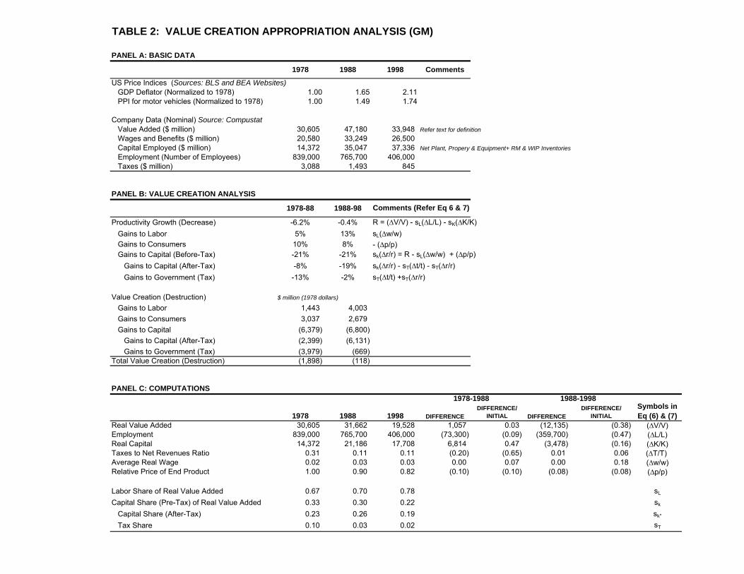
Table 2 presents comparable calculations for General Motors. The pattern of

value creation and distribution at GM contrasts sharply with the pattern at Toyota.

Our analysis shows a 6% decline in total factor productivity for GM over the first

decade of our sample, and a very small -0.4% decline over the second decade.

Hence, we find net value destruction by GM and a decrease in GM’s efficiency of

resource use since the late 1970s.10 Shareholders were particularly hard hit; they

gave up even more than GM’s overall efficiency loss. After-tax gains to capital fell by

10 Note that GM may have created economic value over this period, but our analysis demonstrates that the increment was negative, i.e., GM created less value in 1998 than in 1978.

24

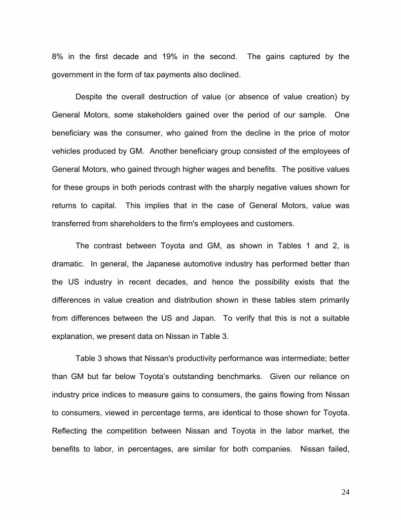
8% in the first decade and 19% in the second. The gains captured by the

government in the form of tax payments also declined.

Despite the overall destruction of value (or absence of value creation) by

General Motors, some stakeholders gained over the period of our sample. One

beneficiary was the consumer, who gained from the decline in the price of motor

vehicles produced by GM. Another beneficiary group consisted of the employees of

General Motors, who gained through higher wages and benefits. The positive values

for these groups in both periods contrast with the sharply negative values shown for

returns to capital. This implies that in the case of General Motors, value was

transferred from shareholders to the firm's employees and customers.

The contrast between Toyota and GM, as shown in Tables 1 and 2, is

dramatic. In general, the Japanese automotive industry has performed better than

the US industry in recent decades, and hence the possibility exists that the

differences in value creation and distribution shown in these tables stem primarily

from differences between the US and Japan. To verify that this is not a suitable

explanation, we present data on Nissan in Table 3.

Table 3 shows that Nissan's productivity performance was intermediate; better

than GM but far below Toyota’s outstanding benchmarks. Given our reliance on

industry price indices to measure gains to consumers, the gains flowing from Nissan

to consumers, viewed in percentage terms, are identical to those shown for Toyota.

Reflecting the competition between Nissan and Toyota in the labor market, the

benefits to labor, in percentages, are similar for both companies. Nissan failed,

25

however, to match Toyota's strong gains to capital; indeed, Nissan's incremental

gains to capital are negative.11 Nissan's tax payments, already smaller than Toyota's

in 1978, declined over the decades of our sample as Nissan's profits fell.

Another possible explanation for the dramatic difference between Toyota and

GM could be that our approach examines the change in value created but not the

level of value creation. Hence, it is possible that in 1978, GM had a much higher

productivity than Toyota, and that in 1998 the two firms had similar productivities.

The patterns in Tables 1 and 2 could arise if Toyota was merely catching up to GM’s

productivity levels. Though our approach does not provide a rigorous test to

compare the levels, we can attempt a crude comparison. In order to do so, we

“expand” Toyota to GM’s size by equating Toyota’s value added to GM’s in 1978 and

multiplying Toyota’s capital and labor by the ratio of GM’s value added to Toyota’s

value added. This is done in Table 4 and Appendix 1. Although the alternative

estimates in the appendix differ in magnitude, they all suggest that GM was slightly

more efficient than Toyota in 1978. This differential, however, is small relative to the

subsequent productivity growth shown for Toyota in Table 1. Hence, the large

differences in value creation (between Toyota and GM) observed in Tables 1 and 2

cannot be linked to an initial difference in productivity levels.

11 Note that the returns to Nissan’s capital owners may have been positive during this period. The negative numbers shown here imply that capital owners did not capture any part of the productivity gains. In fact, competition in the labor and product markets forced Nissan’s capital owners to transfer all the productivity gains (and then some more) to employees and consumers, thus lowering their own returns.

26

6. DISCUSSION

The approach to measurement of value creation and value capture described

above is based on simple accounting identities, and thus it is quite general. In this

section we elaborate on the key assumptions and potential limitations of the model.

Many of these limitations relate to the difficulties of correctly measuring prices and

quantities. We also consider ways that the model and measures can be elaborated.

The methodology itself is purely descriptive and focuses solely on

measurement – it is agnostic about why the firm performs well or poorly, how value is

created and why some stakeholders capture more value than others. Nevertheless,

it provides an empirical tool to examine some of these questions, specifically by

generating quantitative measures of value creation and distribution, which can then

be analyzed. For instance, one could use the approach to estimate the value

captured by consumers and investigate how the magnitude of consumer gains may

be influenced by factors such as industry rivalry, buyer power, technological change,

product characteristics, etc.

Another advantage of our method is its close relation to traditional measures

of firm performance such as return on assets. Specifically, our measure of the gains

to capital (sk Δr/r from Equation 5) represents the part of the additional value added,

achieved through productivity gains, that flows to shareholders. (For simplicity, we

ignore taxes.) This would also equal the incremental cash flow to shareholders. For

instance, consider a firm with a capital (K) of 250 million dollars, and an initial value

added (pY) of 100 million dollars, of which 75 million went to workers as wages and

27

benefits (wL), and 25 million as profits to capital (rK). Then, its initial return on assets

would be 10%. If this firm increased its productivity by 2%, without any change in

output prices, employment, wages or capital stock, the measure, sk Δr/r, would be

2%, since capital owners capture all productivity gains. The new return on assets

can be obtained by adding the incremental 2 million (2% of 100 million) to profits, and

dividing by the capital base to get 10.8%.12 Hence, gains to capital in Equation (5)

will be positively correlated with increased return on assets as measured

traditionally.13

The methodology interprets a quantity that is essentially a “residual”

(Equations 4 and 6) as being the result of productivity improvement efforts by the

firm. In particular, all changes in a firm’s output not explained by changes in input

quantities are attributed to efficiency improvements and hence called “value

creation.” This interpretation, which largely follows the economics literature, is critical

to our methodology and deserves some discussion. For a single-input case, where

productivity can be intuitively defined as the ratio of output to input, the residual is

equivalent to the increase in productivity.14 Equations (4) and (6) are only extensions

12 Given that our calculations for Toyota and GM take the capital stock, K, as a conventional accounting measure of the firm’s assets, r can be interpreted as the gross return on assets. Part of this return represents depreciation; in the illustrative example presented, if the rate of economic depreciation was 10%, the return net of depreciation would initially be zero, rising to 0.8% at the end of the period. 13 Our measures are directly linked to accounting measures of performance, but not to forward looking measures, such as the firm’s stock price and market value. The latter are based upon anticipated returns; in this example, if the 2% productivity gain and its flow to shareholders were fully anticipated, there would be no change in the firm’s market value. 14 Let Y and L be the initial quantities of output and input. If these increase to Y+ΔY

28

to the case of multiple inputs. Hence, if all quantities are correctly measured and

adjusted for quality variations, and if all inputs have been taken into account, the

“residual” can be appropriately interpreted as a productivity gain.

Measurement issues arise because of two closely linked reasons: (a) real

output quantities are not directly observed, and (b) we cannot completely adjust for

quality changes in inputs and outputs. Because the firm’s real output quantity is not

directly observed, we have to infer it indirectly. Firm-specific prices solve this

problem, but they are not normally available. Hence, we divide revenues (or “value

added”) by an industry price index to get a measure of output quantity. However, this

brings to the fore all the difficulties in correctly computing the price index. First, price

indexes are publicly available only at the industry level. If a firm’s product portfolio is

significantly different from the ‘products basket’ used for calculating the index, errors

will creep into the computations of value creation and value distribution. Second, it is

difficult to correctly adjust for improvements in the quality of the output. Ideally, the

price index should reflect quality improvements - for instance, if the (real) dollar price

of a 1 Gigabyte Memory for 2005 is the same as that of a 64 Kilobyte Memory in

1990, then the 2005 memory price index should be many times lower than the 1990

index. Though significant improvements have been made in index computations

using hedonic pricing methods, it is unlikely that adjustment for all quality

improvements can be made. Hence, for industries and firms that make substantial

and L+ΔL, “productivity” changes from p0=(Y/L) to p1=((Y+ΔY)/(L+ΔL)). Assuming the changes are small relative to initial values, it is easy to show that (p1-p0)/ p0= (ΔY/Y)- (ΔL/L). The term on the right hand side is simply the residual R in Equation (3) for a single-input case.

29

gains in output quality over time, our method is likely to understate the magnitude of

value creation and its flow to consumers.

Our use of an industry-specific output price index assumes that the quality-

adjusted prices of all domestic competitors are identical. Product market competition

ensures that such equality is approximately met, but deviations may arise. For

example, firms may undercut the prices of competitors in an effort to gain market

share (or may lose share if they lag the price cuts of rivals). In this case, information

on trends in market share, combined with assumptions about the elasticity linking

market share and relative price, may allow the firm’s price of output to be more

correctly identified. For example, Toyota’s market share gains in the United States in

recent years suggest that the firm has set its quality-adjusted prices below those of

rivals. Moreover, innovative firms may introduce new goods that are highly valued by

consumers. To the extent that these goods are sold in the market at a price premium

that reflects their superior quality and customer valuation, our method will

appropriately capture their value as higher real output. Even so, the price of the

product reflects the willingness-to-pay of the marginal customer; it is possible that

infra-marginal buyers enjoy a large consumer surplus that is not captured by our

method. One example is hybrid cars, where Toyota has been a pioneer. Some

buyers may enjoy very high value from these cars, greatly exceeding their premium

price. Such consumer surplus generated by new and innovative products is not

captured by our model, although it could be estimated in supplementary calculations.

Further potential adjustments relate to the firm’s international domain of

operations. Our accounting data for Toyota and Nissan are limited to the operations

30

of these two firms within Japan. Hence, our use of Japanese price deflators is

appropriate for these companies in our computations. Increasingly, though, Toyota

and Nissan have become global producers. A full analysis of value creation must

include their plants abroad, and particularly, their now-extensive manufacturing

facilities in North America. But to do so adds greater complexity; for example, if data

for different countries are combined, the price deflators should be taken as a blend of

national indexes, adjusted for exchange rates. In the case of General Motors, we

have simply assumed that US price indexes apply across the firm, even though the

GM data include major operations outside the United States.

The inability to observe quality variations in inputs leads to a different type of

error. Suppose GM is able to produce the same number of cars with 10% less labor

only because it re-trained and augmented its workers’ skills. When adjusted for the

improvement in worker quality, there has been no change in the quantity of labor

used and hence, no change in productivity. However, using the number of

employees as the measure of labor input, we see a reduction in the quantity of labor

and consequently, a spurious 10% productivity gain.

Following such worker training, wages may rise, reflecting the improvement in

labor quality as well as the potential exercise of bargaining power. In this case GM

has invested in "human capital" but may need to pay a premium to retain the more

highly skilled employees. Labor unions may be able to influence the magnitude of

this premium. Wages may also rise over time simply because of general labor

market forces. These factors might be distinguished given data on worker training

and shifts in relative wages observed for the firm, its industry, and the overall

31

economy. Even so, in our model it is likely that improvements in worker training and

education will appear as gains in productivity, and such gains will be reflected, at

least in part, in higher wages. Almost certainly, the gains captured by employees at

Toyota, Nissan and GM, as shown in Tables 1, 2 and 3, are partly attributable to such

increases in worker skill and quality.

Another assumption of our calculations is that the GDP deflator corrects for

inflation in the prices of all inputs. This limitation can be overcome by applying

different price indexes to deflate wages, capital stock, etc. For international firms,

though, the problem is less tractable. Some bias is introduced into Table 2 given our

use of U.S. GDP deflators to adjust the wages of GM workers located abroad.

Viewed in perspective, though, these errors are likely to be smaller than those arising

from other sources.

In our empirical approach, gains to consumers are given by reductions in the

firm's output price relative to the GDP deflator. This may appear to be a limitation,

since it suggests that a firm whose output price merely follows the rate of inflation in

the economy will fail to create any value for consumers. However, a broader

perspective shows that a full analysis of gains to consumers must incorporate the

gains they receive as recipients of higher wages and profits. Consider an economy

where all firms achieve identical rates of productivity growth, and the changes in their

output prices are also identical. In such an economy, all product prices move

together, precisely tracking the GDP deflator. It is clear from Equations 4 and 5 that

to accommodate the growth in TFP, wages and returns to capital must rise relative to

output prices. Hence, consumers gain through their dual role as employees and

32

shareholders: they receive higher wages and returns to capital, relative to product

prices. Returns to capital are unlikely to rise indefinitely, so over long periods of time

the productivity gains in an economy flow primarily into higher wages. Indeed, in

most economies the gains enjoyed by consumers come from the reduction in

average prices relative to wages.

"Spillovers" are another reason why our approach will tend to understate the

extent of value creation by innovative firms. Our approach measures only the value

creation that goes to the firm’s own stakeholders. However, a given firm's innovations

can “spill over” to other firms and their stakeholders. For instance, many auto

companies have now adopted key features of the "Toyota production system" and

have greatly improved their efficiency and product quality as a result. Such gains

from dissemination of the Toyota’s basic methods have gone to stakeholders of

Toyota's competitors, with customers likely being the major beneficiaries. These

“spillovers”, though fundamentally attributable to Toyota’s efforts, are excluded from

our estimates of Toyota's value creation because they are not reflected within

Toyota's accounting statements.

Spillovers are one form of market "externality;" other externalities, which may

be positive or negative, are excluded from our analysis. Thus, our analysis fails to

capture the impact of negative externalities such as pollution resulting from the

operation of the firm; if negative externalities are important, our approach will

overstate the firm's true value creation.

Furthermore, our approach does not directly capture one particular mode of

33

value creation: a highly productive firm can create value simply by growing, even if it

achieves no gain in productivity from one period to the next. In such a case, the firm

is not improving its efficiency of resource use – it is simply “replicating” itself. If the

firm grows by taking market share away from less productive rivals, then society

benefits as a result of resources being re-allocated to a firm where they can be

utilized more productively. In our approach, value creation in a given period occurs

only when the firm’s efficiency increases relative to its efficiency in the prior period.

Hence, our approach shows positive value creation only if the firm makes

improvements with regard to its resource-use efficiency. Over long periods of time,

the errors induced by ignoring this simple replication type of value creation are

probably small. Though it is possible that firms grow for short periods without any

improvements in their productivity, it is unlikely that they can continue to grow over

many years without productivity gains.

These considerations suggest that our calculations of value creation by Toyota

are likely to be conservative on balance. Adjustments for Toyota’s positive spillovers,

infra-marginal consumer surplus, growing market share, and international scope

would be expected to yield even larger estimates of value creation than those shown

in Table 1. On the other hand, adjustment for rising labor quality would reduce

Toyota’s estimated productivity gain, but this adjustment is presumably small.

Notwithstanding these problems, the methodology’s usefulness lies in its

ability to offer quantitative insights into the distribution of value among the firm’s

stakeholders. It is particularly useful because none of the current methodologies

used in the strategic management field offer such a possibility, which has constrained

34

a detailed quantitative investigation of questions related to value distribution. The

limitations discussed above only serve as reminders to be careful when interpreting

the quantitative results.

Another important advantage of this method is its flexibility to incorporate

additional stakeholders, should data on them be available. One simple extension of

this model is to decompose “labor” into various components, e.g., by separating out

the CEO (and other top management) as a factor of production.

7. CONCLUSIONS

In this paper we have presented a methodology for estimating the magnitude

of economic value creation and the distribution of value among a firm’s stakeholders.

Using public data on global automotive companies, we have demonstrated how the

methodology can be applied. Our calculations provide quantitative evidence on the

dramatic differences in value creation and distribution between Toyota and General

Motors in recent decades.

In addition to an empirical method, our approach offers a conceptual

framework for understanding value creation and distribution in a precise way. We

have shown that the standard TFP formula, combined with its “dual”, provides such a

framework within the context of the firm's value chain. The TFP formula (Equation 4)

gives the economic value created by the focal firm, whereas the dual (Equation 5)

tracks the flow of this value among stakeholders. The latter include stakeholders

“within” the firm (shareholders and employees), and those located upstream

(suppliers) and downstream (customers) of the firm, along the value chain.

35

Our empirical approach takes into account the realities of tax payments and

the fact that sufficient data on suppliers are seldom available. Thus, the applied

version of our model drops the firm's suppliers as a potential recipient of value but

adds government as a stakeholder in the success of the firm. While this approach

has some limitations as an empirical tool, we have shown that it can be meaningfully

applied for many companies.

The concept of value creation is central to the field of strategic management,

and researchers have paid great attention to the capture of value by internal and

external stakeholders. Yet there has been surprisingly little development of

quantitative methods for broadly representing the creation and distribution of

economic value at the firm level. We believe that our approach offers promise as a

tool for applied research in strategic management. While essential features of our

approach are drawn from the field of economics, economists have shown little

interest in applying this type of analysis at the level of individual firms. The methods

described in this paper have broad applicability for generating firm-level estimates

and for supporting a range of analyses on the determinants of value creation and its

distribution among stakeholders.

36

REFERENCES

Amit R, Zott C. 2001. Value creation in e-business. Strategic Management Journal

22(6-7): 493-520.

Barney JB. 1986. Strategic factor markets - expectations, luck, and business

strategy. Management Science 32(10): 1230-1241.

Bebchuk, L., Grinstein, Y. 2005. The growth of executive pay. Oxford Review of

Economic Policy 21: 283-303.

Bowman, C., Ambrosini, V. 2000. Value creation versus value capture: Towards a

coherent definition of value in strategy. British Journal of Management, 11(1):

1-15.

Brandenberger AM, Stuart H. 1996. Value-based business strategy. Journal of

Economics and Management Strategy 5:5-25.

Castanias RP, Helfat CE. 2001. The managerial rents model: theory and empirical

analysis. Journal of Management 27: 661:678

Coff, RW. 1999. When competitive advantage doesn't lead to performance: The

resource-based view and stakeholder bargaining power. Organization

Science, 10(2): 119-133.

Coff RW. 2005. What is competitive advantage in a multi-stakeholder, inter-temporal

world? Working Paper

Gadiesh O, Gilbert JL. 1998. Profit pools: a fresh look at strategy. Harvard Business

Review May-June: 139-147.

Harberger AC. 1998 Reflections on the growth process. American Economic Review

88(1): 1-32.

37

Harberger AC. 1999. Studying the growth process: A primer in Capital Formation and

Economic Growth, Boskin MJ(eds). Stanford, CA: Hoover Institution.

Hulten, CR. 2000. Total Factor Productivity: A Short Biography. National Bureau of

Economic Research, Working Paper 7471.

Lieberman MB, Chacar A. 1997. Measuring the distribution of returns among

stakeholders. Methods and application to US and Japanese companies. In

Strategic Discovery: Competing in New Arenas. Thomas H, O’Neal D,

Alvarado R (Eds.) John Wiley & Sons: New York.

Lippman SA, Rumelt RP. 2003a. The payments perspective: Micro-foundations of

resource analysis. Strategic Management Journal, 24: 903-927

Lippman SA, Rumelt RP. 2003b. A bargaining perspective on resource advantage.

Strategic Management Journal, 24: 1069-1086

Murphy KJ. 1997. Executive compensation and the modern industrial revolution.

International Journal of Industrial Organization 15(4): 417-426

MARKET DEMAND CURVE

FIRM COST CURVE ( PERIOD 1)


VALUE CREATED (PERIOD 1)

INCREMENTAL VALUE CREATED (PERIOD 2)

FIRM OUTPUT (ASSUMED CONSTANT)

$/U

NIT

FIGURE 1: VALUE CREATION

MARKET DEMAND CURVE



VALUE CREATED (PERIOD 1)

INCREMENTAL VALUE CREATED (PERIOD 2)

FIRM OUTPUT (ASSUMED CONSTANT)

$/U

NIT

FIGURE 1: VALUE CREATION

1978 1988 1998 Comments

Japanese Price Indices (Source: Economic Planning Agency, Bank of Japan)GDP Deflator (1990=100) 76.90 96.00 105.12PPI for motor vehicles (1990=100) 0.963 0.996 0.817GDP Deflator (Normalized to 1978) 1.00 1.25 1.37PPI for motor vehicles (Normalized to 1978) 1.00 1.03 0.85

Company Data (Nominal) Source: Annual Reports (Yuka Shoken Hokokusho)Value Added (Yen million) 430,046 1,115,451 1,514,853 Refer text for definitionWages and Benefits (Yen million) 173,880 431,614 678,894 Capital Employed (Yen million) 404,669 1,019,697 1,457,920 Tangible Fixed Assets + RM & WIP InventoriesEmployment (Number of Employees) 46,477 67,389 67,912 Taxes (Yen million) 117,293 360,684 311,043

PANEL B: VALUE CREATION ANALYSIS

1978-88 1988-98

Productivity Growth (Decrease) 72% 47% R = (∆V/V) - sL(∆L/L) - sK(∆K/K)Gains to Labor 15% 16% sL(∆w/w) Gains to Consumers 17% 25% - (∆p/p)Gains to Capital (Before-Tax) 40% 5% sk(∆r/r) = R - sL(∆w/w) + (∆p/p)

Gains to Capital (After-Tax) 17% 12% sk(∆r/r) - sT(∆t/t) - sT(∆r/r) Gains to Government (Tax) 22% -7% sT(∆t/t) +sT(∆r/r)

Value Creation (Destruction) Million Yen (1978 Yen)

Gains to Labor 64,571 177,537 Gains to Consumers 73,795 270,605 Gains to Capital 171,059 53,597

Gains to Capital (After-Tax) 74,915 128,061 Gains to Government (Tax) 96,144 (74,464)

Total Value Creation (Destruction) 309,425 501,739

PANEL C: COMPUTATIONS

1978 1988 1998 DIFFERENCEDIFFERENCE/

INITIAL DIFFERENCEDIFFERENCE/

INITIALReal Value Added 430,046 1,078,610 1,785,736 648,564 1.51 707,126 0.66 (∆V/V)Employment 46,477 67,389 67,912 20,912 0.45 523 0.01 (∆L/L)Real Capital 404,669 816,820 1,066,526 412,151 1.02 249,706 0.31 (∆K/K)Taxes to Net Revenues Ratio 0.46 0.53 0.37 0.07 0.15 (0.16) (0.29) (∆T/T) Average Real Wage 3.74 5.13 7.31 1.39 0.37 2.18 0.43 (∆w/w)Relative Price of End Product 1.00 0.83 0.62 (0.17) (0.17) (0.21) (0.25) (∆p/p)

Labor Share of Real Value Added 0.40 0.39 0.45 sL

Capital Share (Pre-Tax) of Real Value Added 0.60 0.61 0.55 sk

Capital Share (After-Tax) 0.32 0.29 0.35 sk*

Tax Share 0.27 0.32 0.21 sT

TABLE 1: VALUE CREATION APPROPRIATION ANALYSIS (TOYOTA)

PANEL A: BASIC DATA

1978-1988Symbols in Eq (6) & (7)

Comments (Refer Eq 6 & 7)

1988-1998

1978 1988 1998 Comments

US Price Indices (Sources: BLS and BEA Websites)GDP Deflator (Normalized to 1978) 1.00 1.65 2.11PPI for motor vehicles (Normalized to 1978) 1.00 1.49 1.74

Company Data (Nominal) Source: CompustatValue Added ($ million) 30,605 47,180 33,948 Refer text for definitionWages and Benefits ($ million) 20,580 33,249 26,500 Capital Employed ($ million) 14,372 35,047 37,336 Net Plant, Propery & Equipment+ RM & WIP InventoriesEmployment (Number of Employees) 839,000 765,700 406,000 Taxes ($ million) 3,088 1,493 845


1978-88 1988-98

Productivity Growth (Decrease) -6.2% -0.4% R = (∆V/V) - sL(∆L/L) - sK(∆K/K)Gains to Labor 5% 13% sL(∆w/w) Gains to Consumers 10% 8% - (∆p/p)Gains to Capital (Before-Tax) -21% -21% sk(∆r/r) = R - sL(∆w/w) + (∆p/p)

Gains to Capital (After-Tax) -8% -19% sk(∆r/r) - sT(∆t/t) - sT(∆r/r) Gains to Government (Tax) -13% -2% sT(∆t/t) +sT(∆r/r)

Value Creation (Destruction) $ million (1978 dollars)

Gains to Labor 1,443 4,003 Gains to Consumers 3,037 2,679 Gains to Capital (6,379) (6,800)

Gains to Capital (After-Tax) (2,399) (6,131) Gains to Government (Tax) (3,979) (669)

Total Value Creation (Destruction) (1,898) (118)




INITIALReal Value Added 30,605 31,662 19,528 1,057 0.03 (12,135) (0.38) (∆V/V)Employment 839,000 765,700 406,000 (73,300) (0.09) (359,700) (0.47) (∆L/L)Real Capital 14,372 21,186 17,708 6,814 0.47 (3,478) (0.16) (∆K/K)Taxes to Net Revenues Ratio 0.31 0.11 0.11 (0.20) (0.65) 0.01 0.06 (∆T/T) Average Real Wage 0.02 0.03 0.03 0.00 0.07 0.00 0.18 (∆w/w)Relative Price of End Product 1.00 0.90 0.82 (0.10) (0.10) (0.08) (0.08) (∆p/p)




Tax Share 0.10 0.03 0.02 sT

Symbols in Eq (6) & (7)

TABLE 2: VALUE CREATION APPROPRIATION ANALYSIS (GM)

1978-1988

PANEL A: BASIC DATA


1988-1998

1978 1988 1998 Comments

Japanese Price Indices (Source: Economic Planning Agency, Bank of Japan)GDP Deflator (1990=100) 76.90 96.00 105.12PPI for motor vehicles (1990=100) 0.963 0.996 0.817GDP Deflator (Normalized to 1978) 1.00 1.25 1.37PPI for motor vehicles (Normalized to 1978) 1.00 1.03 0.85

Company Data (Nominal) Source: Annual Reports (Yuka Shoken Hokokusho)Value Added (Yen million) 412,912 560,552 459,614 Refer text for definitionWages and Benefits (Yen million) 220,238 335,204 331,617 Capital Employed (Yen million) 440,544 633,259 795,435 Tangible Fixed Assets + RM & WIP InventoriesEmployment (Number of Employees) 56,068 52,808 39,467 Taxes (Yen million) 78,485 79,556 5,796


1978-88 1988-98

Productivity Growth (Decrease) 27% 9% R = (∆V/V) - sL(∆L/L) - sK(∆K/K)Gains to Labor 16% 12% sL(∆w/w) Gains to Consumers 17% 25% - (∆p/p)Gains to Capital (Before-Tax) -6% -28% sk(∆r/r) = R - sL(∆w/w) + (∆p/p)

Gains to Capital (After-Tax) -1% -6% sk(∆r/r) - sT(∆t/t) - sT(∆r/r) Gains to Government (Tax) -5% -22% sT(∆t/t) +sT(∆r/r)

Value Creation (Destruction) Million Yen (1978 Yen)

Gains to Labor 64,850 67,698 Gains to Consumers 70,855 135,988 Gains to Capital (22,955) (154,093)

Gains to Capital (After-Tax) (3,140) (32,632) Gains to Government (Tax) (19,815) (121,462)

Total Value Creation (Destruction) 112,750 49,593




INITIALReal Value Added 412,912 542,038 541,801 129,126 0.31 (237) (0.00) (∆V/V)Employment 56,068 52,808 39,467 (3,260) (0.06) (13,341) (0.25) (∆L/L)Real Capital 440,544 507,267 581,892 66,723 0.15 74,625 0.15 (∆K/K)Taxes to Net Revenues Ratio 0.41 0.35 0.05 (0.05) (0.13) (0.31) (0.87) (∆T/T) Average Real Wage 3.93 5.08 6.15 1.16 0.29 1.06 0.21 (∆w/w)Relative Price of End Product 1.00 0.83 0.62 (0.17) (0.17) (0.21) (0.25) (∆p/p)




Tax Share 0.19 0.14 0.01 sT

1988-1998Symbols in Eq (6) & (7)

TABLE 3: VALUE CREATION APPROPRIATION ANALYSIS (NISSAN)

PANEL A: BASIC DATA


1978-1988

Toyota GM Toyota (Expanded)

Exchange RateYen to US $ 210.46

Company Data (Real=Nominal in 1978 prices)Value Added ($ million) 2,043 30,605 30,605 Wages and Benefits ($ million) 826 20,580 12,375 Capital Employed ($ million) 1,923 14,372 28,799 Employment (Number of Employees) 46,477 839,000 696,128 Taxes ($ million) 557 3,088 8,347

Assign GM's RoR to ToyotaToyota's actual RoR 0.34 Toyota's assigned RoR 0.48 Toyota's return to capital at actual RoR 9,883 Toyota's return to captial assigned RoR 13,901 Additional value to be created by Toyota 4,017 % difference 13% GM's productivity is 13% higher than Toyota's

Assign Toyota's RoR to GMGM's actual RoR 0.48 GM's assigned RoR 0.34 GM's return to capital at actual RoR 6,937 GM's return to captial assigned RoR 4,932 Additional value to be created by GM (2,005) % difference -7% Toyota's productivity is 7% lower than GM's

Toyota numbers subtracted from GM numbers Change in Real Value Added - Change in Employment 0.17 Change in Real Capital Employed (1.00) Average Labor Share 0.54 Average Capital Share 0.46

% Productivity Difference 37% GM's productivity is 37% higher than Toyota'sGM numbers subtracted from Toyota numbers

Change in Real Value Added - Change in Employment (0.21) Change in Real Capital Employed 0.50 Average Labor Share 0.54 Average Capital Share 0.46

% Productivity Difference -12% Toyota's productivity is -12% lower than GM's

TABLE 4: COMPARISON OF TOYOTA AND GM (1978)

METHOD 1 (EQUATING RATE OF RETURN ON CAPITAL)

METHOD 2 (USING EQUATIONS 6 AND 7)

Appendix 1: Comparison of GM and Toyota in 1978

To compare GM’s and Toyota’s productivity levels, we can use one of two

approaches, both of them only offering approximate answers. The first approach

would be to simply assign the same rate of return on capital (say, defined as value

added less wages less taxes divided by capital employed) for both Toyota and GM

and compute the excess (or shortfall in) value created. Hence, we could assign a

48% rate of return (which is GM’s rate of return on capital) to Toyota. This would

imply Toyota would have to pay $ 13,901 million on its capital, which would mean its

current value added is short by $4,017 million, or about 13% of its “expanded” value

added (Table 4). Hence, in some sense, GM’s productivity in 1978 is about 13%

higher than Toyota’s productivity then. Alternatively, we could assign Toyota’s rate of

return (34%) to GM and compute the excess value added by GM. This turns out to

be about 7% of GM’s value added. Based on this, Toyota’s productivity is about 7%

lower than GM’s productivity.

An alternate approach is to “expand” Toyota to GM and use Equation (3) with

the changes taken across GM and Toyota rather than over time for a single firm. We

use this approach along with the average input shares to compute the productivities.

Once again, we can have two comparisons, by subtracting GM from Toyota (i.e.

“convert GM to Toyota”) or subtracting Toyota from GM (i.e. convert Toyota to GM).

Based on this approach, GM’s productivity in 1978 turns out to be 37% more

productive than Toyota if Toyota is used as the starting point or Toyota’s about 12%

lower than GM, if we use GM as the initial point. Though imprecise, both approaches

suggest that GM was using resources only a bit more efficiently than Toyota in 1978.

measuring value creation and its distribution among stakeholders

Documents