measuring the impact of multiple air-pollution agreements

Economics Working Paper Series

2014/010

Measuring the impact of multiple air-pollution

agreements on global CO2 emissions

Aurélie Slechten and Vincenzo Verardi

The Department of Economics Lancaster University Management School

Lancaster LA1 4YX UK

© Authors All rights reserved. Short sections of text, not to exceed

two paragraphs, may be quoted without explicit permission, provided that full acknowledgement is given.

LUMS home page: http://www.lums.lancs.ac.uk/

Measuring the impact of multiple air-pollution

agreements on global CO2 emissions

Aurelie Slechten∗and Vincenzo Verardi‡

June 2014

Abstract

Many countries are part of multiple international air-pollution agreements

that interact with each other given that a single source of emissions is typi-

cally composed of several pollutants. This paper studies the effect on carbon

dioxide emissions of the various agreements that follow the Long-Range Trans-

boundary Air-Pollution (LRTAP) Convention and that are related to acid rain

problems. The analysis is based on a panel dataset of 150 countries over the

period 1970 - 2008. We show that ratifying each additional treaty has a signif-

icant and negative impact on the level of CO2 emissions, even if they are not

specifically targeted toward carbon emissions. Our findings can be explained

by (1) the more local nature of pollutants covered (2) the relative ease to im-

plement LRTAP treaties. To deal with an eventual reverse causality problem,

we instrument the decision to ratify treaties by the status of the death penalty

in each country.

Keywords: Air-pollution Agreements; CO2 emissions; Panel data

JEL Codes: Q53, Q54

∗Corresponding author: Lancaster University Management School, Bailrigg, Lancaster, LA1

4YW, United Kingdom (e-mail: [email protected]).‡CRED (Center for Research in Economic Development), University of Namur, Rempart de la

Vierge, 8, B-5000 Namur, Belgium (e-mail: [email protected]).

1

1 Introduction

The starting point of this paper is that many countries are part of multiple en-

vironmental agreements and that these agreements may interact with each other

given that they focus on externalities that are correlated. Our goal is to show that

studying the effect of one agreement in isolation may thereby be misleading.

International mechanisms to control transboundary externalities have received

increasing attention from policy-makers and scholars, driven by the acknowledgment

of global problems such as climate change or ozone layer depletion as well as more re-

gional problems associated with acid rains. A common feature of these international

mechanisms is that they are generally designed to control emissions of one single

pollutant. For example, the Kyoto Protocol aims at reducing carbon dioxide (CO2)

emissions, the main cause of global warming, while more conventional air-pollutants

(e.g. sulfur dioxide SO2, nitrogen oxide NOx or volatile organic compounds VOC)

are the targets of international treaties that follow the 1979 Convention on Long-

Range Transboundary Air-Pollution (the 1979 LRTAP Convention, hereafter).

In reality, a single source of emissions is typically composed of multiple pollutants

that simultaneously cause global and/or more regional environmental damages. For

example, Barker (1993, p. 9) calculated that in the United Kingdom, the burning of

fossil fuels is responsible, apart from CO2 (which creates global externalities) for over

99% of SO2 and NOx, 91% of particulate matter and 38% of VOC emissions, which

imply more regional or local environmental damages (e.g. acid rains, degradation of

ambient air quality). This pattern is also true in other countries (see OECD, 1991,

p. 36).

As they are emitted by a single source, existing abatement technologies may have

joint effects on this multiplicity of pollutants. These effects can go in both direction.

Consider the case of acid rains control. Among the options available to reduce SO2

emissions, substituting high sulfur by low sulfur coal would imply carbon reductions

as a by-product. In the same way, switching from burning coal to burning natural

gas would imply SO2 and NOx reductions, as well as CO2 reductions. On the other

hand, scrubbers installed in power plants to neutralize SO2 or NOx use energy and,

therefore, lead to more CO2 emissions.

All in all, the fact that many production processes emit multiple pollutants and

2

current abatement technologies are coarse implies that a number of important pol-

lution problems are correlated. As a consequence, an international treaty foreseeing

abatement of one of these air-pollutants may also have a significant impact on the

other pollutants. In this paper, we analyze the case of international treaties that

follow the 1979 LRTAP Convention and that address conventional air-pollutants

such as SO2, NOx or VOC. As these pollutants are very often released jointly with

CO2 emissions, these agreements may have an indirect impact on carbon emissions,

even if they are not CO2-specific. This question has important implications for the

design of future international agreements because it alters the cost-benefit calcu-

lations underlying policy targets. Among others, the economic literature is very

skeptical about the effectiveness of the current climate international policies, e.g.

the Kyoto Protocol (see for example Barrett, 2003 or Bohringer and Vogt, 2004). In

this paper, we argue that looking at one agreement in isolation is not sufficient. In

order to build an optimal climate change policy it is important to understand the

interactions between other non CO2-specific treaties and the level of CO2 emissions.

Identifying the effect of an agreement raises two problems: (1) reverse causality

since countries’ incentives to ratify agreements may depend on their emission levels

and (2) timing effects of the treaty (i.e. effects may start early or be bunched

at a future date). As we analyze the effect of multiple treaties, the identification

challenge becomes higher because they overlap in time and in terms of signatory

countries. There may not be sufficient heterogeneity between them to identify their

individual effects.

Getting the causality right is crucial in order to derive policy implications from

the empirical results. We deal with the problem of reverse causality by instru-

menting the decision to ratify an air-pollution agreement using the status of the

death penalty. We believe that universalism, i.e. the conviction that some system

of ethics should apply universally, can explain the decision to ratify international

treaties without affecting the level of CO2 emissions directly. The idea is that a uni-

versalist country ratifies an international agreement not because of its subject but

because it is an international policy initiative and that it values such initiatives. We

also believe that the abolition of the death penalty is a good proxy for universalism

or progressivism.

We deal with timing effects and time and membership overlap issues together.

3

Since agreements that follow the 1979 LRTAP Convention are relatively similar in

terms of their timing and signatory countries, it is impossible to identify the effects of

these agreements individually. One contribution of this paper consists in proposing

a new methodology to overcome these issues: we group LRTAP treaties into a single

variable. The idea behind this assumption is that agreements related to the same

air-pollution issue (i.e. here acid rains) are linked and should have a similar impact

on CO2 emissions.

Interestingly, LRTAP treaties are associated with statistically significant CO2

emissions reductions. This result indicates that the options used to reduce SO2 or

NOx emissions imply carbon reductions as a byproduct (e.g. fuel switching or use

of low sulfur coal). An interesting question is why these LRTAP agreements seem

to have been effective in reducing carbon emissions, while a CO2-specific treaty

as the Kyoto Protocol has been considered as poorly effective in the literature.

We suggest two interpretations based on the nature of LRTAP treaties to explain

their effectiveness. First, SO2 and NOx are more local pollutants, compared to

CO2. Intuitively, local agreements imply a higher commitment than more global

agreements: politicians have a greater incentive to set more ambitious targets for

local pollutants (and indirectly for CO2 as a by-product), because the effects of this

pollution are more visible to the voters. Second, acid rain agreements are easier

to implement than the Kyoto Protocol. Indeed, their texts are more focused and

contain not only clear targets, but well identified means to meet these targets.

The approach used in this paper differs from the existing empirical literature on

international environmental agreements (Murdoch and Sandler, 1996; Bratbeg et al.,

2005; Aakvik and Tjøtta, 2011) by considering multiple non CO2-specific agreements

at the same time, instead of focusing on a single one. It points out the limitations

of studying the effects of each treaty in isolation. In line with this idea, Egger

and Wamser (2012) challenge the existing literature on preferential agreements,

which focuses on one policy area, by providing evidence of an important overlap

in the conclusion of different types of preferential economic integration agreements.

They emphasize the difficulty of examining the impacts of these treaties in isolation

from each other. Some papers deal with potential interactions between air-pollution

policies and their ancillary benefits, but they are either purely theoretical models

(Ambec and Coria, 2013 or Caplan and Silva, 2005) or numerical simulations, e.g.

4

integrated cost-benefit analyses (Burtraw et al., 2001 or Bollen et al., 2009).

The structure of the paper is the following: section 2 describes the data and the

identification strategy. Section 3 reports the results for different specifications. The

results are then discussed in section 4. A sensitivity analysis is presented in section

5. Section 6 concludes.

2 Data and identification strategy

The aim of this paper is to study whether a country’s participation in a non CO2-

specific air-pollution agreement has an impact on the level of CO2 emissions of that

country. In this section, we first describe our emissions and air-pollution treaties

data. We then turn to the identification issues raised by our question.

2.1 Data

We use a panel dataset that covers 150 countries and 38 years (1970-2008). Data

on CO2 emissions (in kilotons) come from the World Development Indicator (WDI)

Dataset (World Bank, 2012).1 These data only include CO2 emissions from energy-

related sources (approximately 70 per cent of total anthropogenic CO2 emissions,

see Stern, 2006).2

A single source of CO2 emissions is generally also responsible for other air-

pollutants emissions. The typical examples are the so-called conventional air pol-

lutants, e.g. SO2, NOx or VOC (see Barker, 1993). To select the international

agreements targeting air-pollutants released with CO2 emissions in most industrial

processes, we refer to the International Environmental Agreements Database Project

(Version 2012.1, see http://iea.uoregon.edu/). It provides for each country a list of

the environmental agreements in which the country is involved, with the signature,

ratification and entry into force dates, and when relevant the withdrawal date.3 In

1http://data.worldbank.org/data-catalog/world-development-indicators.2Note that those data do not take into account CO2 emissions/removals from land use, land

use change and forestry, LULUCF (IEA, 2010). We will try to control for this in the sensitivity

analysis in section 5.3A treaty is defined as “an intergovernmental document intended as legally binding with a

primary stated purpose of preventing or managing human impacts on natural resources”. A de-

5

the IEA Database, the agreements of interest for this analysis belong to the Long-

Range Transboundary Air-Pollution lineage, which consists of one initial convention,

8 protocols and 15 amendments and that are targeted to conventional air-pollutants,

responsible for acid rains or degradations in ambient air quality.

This lineage started with the 1979 Convention on Long-Range Transboundary

Air Pollution, which followed increasing concerns by policy-makers about the harm-

ful effect of transboundary pollution caused by SO2 or NOx emissions that can travel

some hundreds of kilometers before deposition. This initial Convention served as

a basis for eight follow-up protocols and a series of amendments. In our analysis,

we cannot include all these treaties because they are not all comparable. We only

include those that satisfy the three following criteria: (1) the objective of the treaty

is the reduction of emissions of some air-pollutant, (2) the treaty includes explicit

emission reduction targets (i.e. it is not a fine proclamation), and (3) it should

involve the country (i.e. it should not rely on the tacit acceptance procedure).4

The 15 amendments rely on the tacit acceptance procedure and are thus deleted

(these are mainly technical modifications of the original treaty). The initial 1979

LRTAP Convention is also dropped because it does not include explicit targets. It

only provides for the establishment of institutions entitled to negotiate the subse-

quent protocols. For the same reason, the 1984 monitoring and evaluation protocol

EMEP, which only requires that signatories report their emissions to the treaty sec-

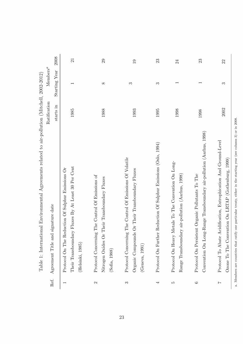
retariat, is also dropped. We are left with seven treaties related to air-pollution

that include emissions reductions targets for ratifying countries. Details on these

agreements can be found in Table 1.

[INSERT TABLE 1 HERE]

We will assume that an agreement’s year of ratification in national parliaments

is the point in time from which this agreement has an impact on emissions. Rati-

fication is preferred to signature because ratification involves political parties, the

scription of the database is given in Mitchell (2003).4This procedure is used to adopt urgently needed amendments to international environmental

agreements. The body that adopts this amendment at the same time fixes a specific time within

which the parties will have to opportunity to notify either their acceptance or rejection or to remain

silent. In case of silence the amendment is considered as accepted by the party.

6

media, and the general public, while the signature of an agreement has no imme-

diate political relevance. This choice is in line with other empirical analyses of

international environmental agreements (e.g. Bratberg et al., 2005 or Aichele and

Felbermayr, 2012): there exists some anecdotal evidence that countries have en-

gaged in policy initiatives after the ratification of an agreement and before its entry

into force.5

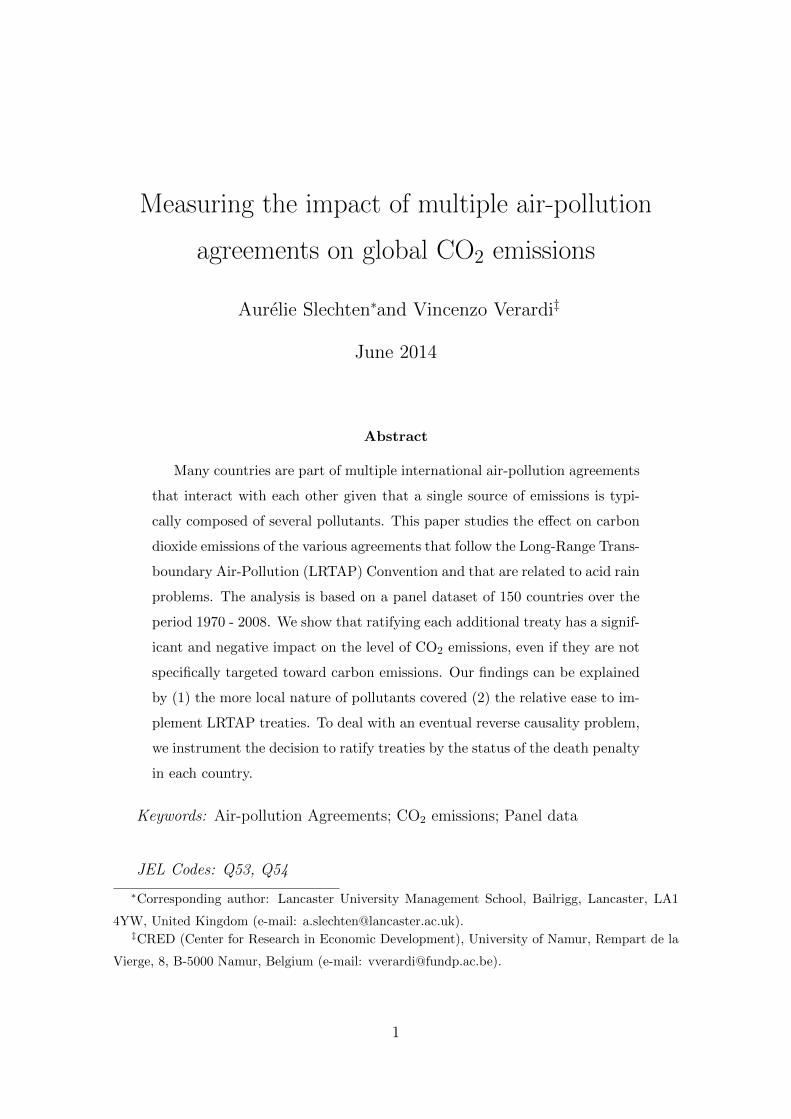
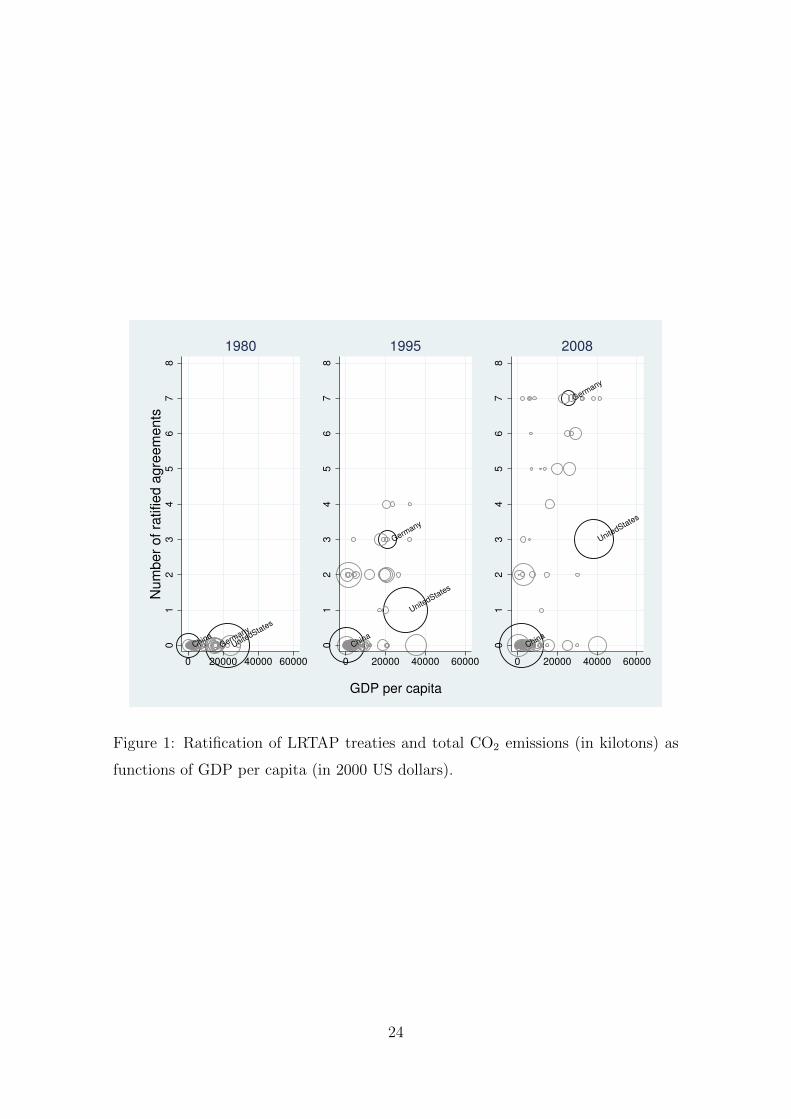
Figure 1 shows the number of ratified LRTAP agreements by country as a func-

tion of GDP per capita. Each country is represented by a bubble, the size of which

represents the level of CO2 emissions. Among the 150 countries of the sample, there

is a lot of heterogeneity in terms of ratification behavior.

[INSERT FIGURE 1 HERE]

European countries (centered around Germany in Figure 1) are the ones that

have ratified the largest number of agreements. The gap in the number of rati-

fications between the United States (US) and Europe has increased sharply since

1995. Figure 1 also shows that both Europe and the US have reduced their emis-

sions between 1995 and 2008. China’s emissions have increased sharply during this

period, while the number of agreements ratified by this country remained at zero.

From Figure 1, one might believe that it is because European countries have ratified

many treaties that they were able to reduce their emissions while China and the US

still accounted for approximately 40% of total world emissions in 2008.

2.2 Identification strategy

The first insights from Figure 1 do not account for the fact that the changes in

the emission behavior can be due to spuriousness: other variables can explain the

emission behavior of the ratifiers. Additionally to confounding effects, we need to

deal with four problems when identifying the effects of multiple agreements on CO2

emissions: (1) time and membership overlap (is there sufficient variation in terms of

5As a robustness check in the Results section, we also use a different definition of our variable

of interest: an air-pollution agreement starts to matter after the treaty’s entry into force. This

does not change our results. The reason is that due to the setting of LRTAP treaties, ratification

and entry into force coincide (almost to the year) for many countries in our sample.

7

treaties’ timing and signatory countries), (2) timing effects (the effect of an agree-

ment does not necessarily occur immediately after its ratification) (3) persistence

of CO2 emissions (due to the substantial inertia of some of CO2, it is plausible to

assume that this year’s CO2 emissions are dependent on the CO2 emissions of pre-

vious years), and (4) reverse causality since countries’ incentives to ratify treaties

may depend on their emission levels. We detail below how we overcome these issues.

2.2.1 Controlling for confounding effects

Spuriousness can be checked for by making use of control variables. The following

model examines how CO2 emissions react to the ratification of air-pollution agree-

ments controlling for other variables:

log(CO2)it = αi + δt + βXkit−1 + Zitγ + εit (1)

In equation (1) i denotes the country and t the year. Variables are defined

as follows: log(CO2)it is the log of total CO2 emissions of country i in year t (in

kilotons).6 αi is the country fixed effect, δt is the time fixed effect. These fixed effects

control for unobservable country-heterogeneity and common time-varying effects

that could affect emissions. Controlling for unobserved heterogeneity is needed to

capture factors such as country specific technology, regulation or ideology or world

business cycles. The variable of interest Xkit−1 is a dummy variable, where k is the

reference number of the agreement in Table 1, defined as:7

Xkit−1 =

1 if country i has ratified the agreement k by time t− 1

0 otherwise

The variable of interest is considered with one year lag in equation (1) to respect

the timing of events (treaties are not systematically ratified on the first of January).

6Due to our log specification, the coefficients would have remained unchanged by taking CO2

emissions per capita instead of total CO2 emissions as the dependent variable. The only exception

would have been the coefficient of the control variable Population.7By using a within analysis rather than a between analysis, we may underestimate the effect

of treaties on CO2 emissions. We also run a pooled regression (using some additional control

variables) and find stronger results. However, since time invariant omitted variables that may

affect the level of CO2 emissions can be numerous, we prefer to concentrate on within variations

in the rest of the paper.

8

β is the coefficient of interest. It represents the yearly average effect of the ratifi-

cation of an agreement k by country i on this country i’s emissions compared to

business-as-usual emissions after controlling for a set of covariates. This coefficient

may be positive or negative depending on the options used to curb conventional

air-pollutants (e.g. scrubbers or fuel-switching).

Zit is the matrix containing the control variables, for which summary statistics

are presented in Table 11 in appendix A. Data are available from the WDI Database

(World Bank, 2012) and the Polity IV Database.8 The first economic factor that

we include as a control variable is total Gross Domestic Product (GDP). The GDP

data are reported in constant 2000 US dollars. We expect a significant positive

relationship between GDP and emissions. The intuition is simple: a higher economic

activity induces, ceteris paribus, a higher level of pollution due to increased resource

use and waste generation (Panayotou, 1997; Stern, 2002).9 We also include the

GDP growth rate to account for the short term variations in the economic activity

(business cycles). Indeed, following van Vuuren and Riahi (2008), economic growth

is expected to have both a positive effect on CO2 emissions (due to the increase in

energy demand) and a negative effect (due to the improvement in energy efficiency).

Following the international trade literature (see for example Copeland and Tay-

lor, 2004), trade openness is assumed to affect the level of CO2 emissions in two

different ways: (i) increased trade may result in more CO2 emissions due to an

enhanced economic activity, (ii) increased trade may result in reduced CO2 emis-

sion because countries face greater competitive pressure and become more efficient

in resource use (Cole, 2004). We define trade openness as the sum of exports and

imports of goods and services divided by GDP.

Next, we control for the total population given that population size may con-

tribute to CO2 emissions through increased energy demand from the power, industry

or transport sectors (see Li and Reuveny, 2006; Shi, 2002). Since the composition

of the economic activity may also influence the level of CO2 emissions (see Stern,

8http://www.cidcm.umd.edu/inscr/polity/.9The Environmental Kuznets Curve (EKC) hypothesizes an inverse-U shaped relationship be-

tween a country’s per capita income and its level of environmental quality (Galeotti et al., 2006;

Friedl and Getzner, 2003). We test the EKC hypothesis by assuming a quadratic functional form

for GDP in our specification but the main results remain unchanged.

9

2002), we include the shares of agricultural and industrial productions in GDP.

Indeed, industrial and agricultural sectors are more resource-intensive than the ter-

tiary sector. Our last control variable is the Democracy indicator available from the

Polity IV Database, which measures countries’ institutionalized democracy. It is an

additive eleven-point scale (0-10), zero being the worst situation for democracy (see

Congleton, 1992).

2.2.2 Time and membership overlap

To correctly identify the effects of the seven LRTAP treaties included in the analysis,

there must be sufficient heterogeneity in terms of the timing of the agreements and

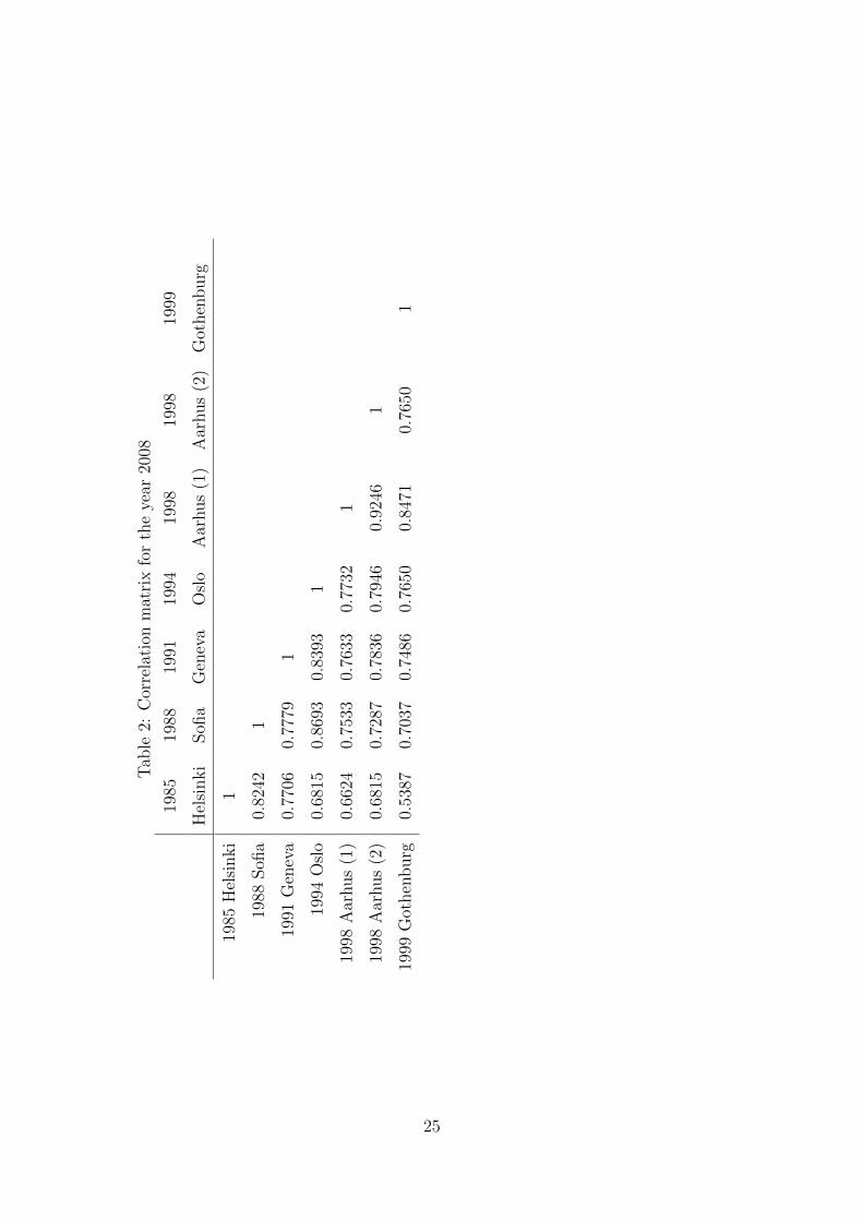
in terms of the ratifying countries. To check for this, we refer to Tables 1 and 2.


First, as shown in Table 1, the number of ratifiers at the end of our sample period

is roughly similar for all LRTAP agreements (i.e. it ranges from 19 to 29). Moreover,

the identity of the ratifiers is also much the same across them. This can be seen from

Table 2, which reports the correlations between the dummies Xki for the year 2008

(the last year of our sample, and thus the year for which the membership overlap

is the highest). These correlations are very high (e.g. above 0.7 for most pairs of

treaties), indicating a low heterogeneity in terms of membership between LRTAP

protocols. Second, the time overlap issue can be seen from Table 1. Treaties have

been ratified since the end of the 1980s until 2005, but the time span between two

agreements is relatively short (generally less than 5 years).

Due to this double overlap, identifying the effect of each individual agreement is

problematic because we cannot be sure that the impact captured is really the impact

of the agreement analyzed. We thus aggregate the agreements in a single variable.

Our argument behind this strategy can be found in their patterns of development.

Countries first agree on an umbrella convention, i.e. the 1979 LRTAP Convention

under the auspices of which all subsequent protocols and amendments are negotiated.

These protocols are thus related. We create a new variable, LRTAPit−1, which is

the sum of dummies Xkit−1 (k = 1, ...7) for country i in year t − 1, and we replace

Xkit−1 by LRTAPit−1 in equation (1).

10

With this definition, we look at the effect of the accumulation of treaties. Our

intuition is the following: the sources of anthropogenic greenhouse gas emissions

are various. A unique air-pollution treaty can only tackle one part of these sources.

By ratifying additional agreements, countries might complete the initial one and

control other sources of emissions. From Figure 1, it can be seen that the variable

LRTAP varies over time and between countries. Moreover, this is confirmed by an

ANOVA analysis of the LRTAP variable: in both case, we reject the null hypothesis

that there is no variation between countries and through time (within a country)

as the F-statistics are respectively of F(149,5662)=26.69 (with p-value 0.00) and

F(38,5662)=28.70 (with p-value 0.00) for countries and years.

2.2.3 Timing effects

To analyze the timing issue, we refer to Table 3, which reports the dates at which

emission targets foreseen in agreements should be met. It is possible that the effect

of an agreement does not occur immediately after its ratification, i.e. implementing

domestic air-pollution control policies may take time. Moreover, as shown in Table

3, treaties generally foresee a schedule for emission reductions. Since our sample

ends in 2008, we may fail to correctly identify the effects of some recent treaties,

e.g. the Gothenburg Protocol. Our counting measure of air-pollution treaties should

allow us to deal with this problem, as the targets of the first agreements should be

met before 2000.


2.2.4 Persistence of CO2 emissions

Equation (1) is in some sense static. Due to the substantial inertia of the dependent

variable, it is plausible to assume that this year’s CO2 emissions are dependent on

the CO2 emissions of previous years. This is why we introduce a lagged dependent

variable in our model:

log(CO2)it = αi + δt + ρ log(CO2)it−1 + βLRTAPit−1 + Zitγ + εit (2)

ρ is the coefficient of the lagged dependent variable. The coefficients of the

explanatory variables, β and γ, have different interpretations compared to the pre-

11

vious basic static specification. They are the estimated responses of CO2 emissions

to changes in the explanatory variables, after controlling for the response for the

previous years.

Some econometric problems arise from estimating equation (2): CO2 may be non-

stationary and the lagged dependent variable is correlated with the error term (due

to the fixed-effect model). The coefficients of the regressors may thus be seriously

biased when estimating equation (2) with OLS. Note however that this bias decreases

when the number of periods becomes large.

Taking the first difference transformation removes the individual effects and al-

lows to deal with non-stationarity, but the correlation between the differenced lagged

dependent variable and the differenced disturbance process is still not zero. To avoid

this problem we estimate the following model using the Anderson-Hsiao (AH) esti-

mator:

∆log(CO2)it = δt − δt−1 + ρ ∆log(CO2)it−1 + β∆LRTAPit−1 + ∆Zitγ + ∆εit (3)

where ∆log(CO2)it−1 is instrumented using lags 2 to 4 of log(CO2)it.

Arellano and Bond (1991) argue that the AH estimator, while consistent, fails

to exploit all the information available in the sample. For this reason, we also

estimate equation (3) using the Arellano-Bond estimator. The AB estimator sets

up a generalized method of moments (GMM) problem in which the model is specified

as a system of equations, one per time period, where the instruments applicable to

each equation differ (for example, in later time periods, additional lagged values of

the instruments are available). By doing so in a GMM context, we construct more

efficient estimates of the dynamic panel data model (3).

2.2.5 Dealing with reverse causality

A reverse causality between the ratified agreements and CO2 emissions may also

explain the stylized facts of Figure 1. It is precisely because they are not the biggest

polluters that European countries participate in many agreements (as they do not

pollute much, it is not very costly for them to ratify many treaties). China and

the US, on the other hand, are reluctant to ratify more agreements because this

would be very costly in terms of emission reductions. The Instrumental Variable

(IV) approach solves this problem by exploiting the exogenous variations in an

12

instrumental variable that is correlated with the endogenous variable of interest

but independent of the error term. When the IV strategy is valid, it allows causal

inference.

In our case, the endogenous variable of interest is the ratification of air-pollution

treaties. The instrument we use is an index that measures the status of the death

penalty. It is constructed as follows:10 we measure the status of the death penalty

on a five-point scale (0-4), from constitutional authorization of the death penalty

(0) to abolition of the death penalty for any offense in both peace and war periods

(4) (see Table 4 for details on scores).

We argue that this is a valid instrument for the four following reasons that will

be detailed below: (1) it is a relevant instrument to measure the propensity of a

country to ratify air-pollution agreements, (2) the status of the death penalty does

not affect the level of CO2 emissions, (3) the level of CO2 emissions does not influence

the countries’ decisions about the death penalty, and (4) the index varies sufficiently

over time and across countries.

First, the pace at which a country ratifies international environmental agreements

may be explained by its universalism, i.e. the meta-ethical conviction that some

system of ethics applies universally (e.g. for every individual, independently of

their culture, religion, nationality, sexuality,...). Indeed, a country that is strongly

universalist will be more keen to ratify international agreements related to public

goods because these treaties are ways to apply this system of ethics universally.

Our idea is to use universalism as an instrument for treaties’ ratification that is

not directly related to CO2 emissions. We believe that the pace at which the death

penalty is abolished, but also the legalization of homosexual marriage or euthanasia,

can be seen as symbols, and therefore as proxies, for progressive or universalist

societies.

Second, this instrument does not affect the level of CO2 emissions directly and

it is obviously not caused by the level of CO2 emissions. However, there may be

a concern that the abolition of the death penalty might be driven by economic

development, which in turn correlates with CO2 emissions. We believe this should

not be a major concern. On the one hand, we control for economic development in

10Amnesty International provides up-to-date information as to the status of the death penalty

for 197 countries.

13

our analysis through our control variable GDP. On the other hand, there is some

anecdotal evidence that this is not always the case: the United States and Japan,

which are already very developed countries (they are amongst the countries with the

highest GDP per capita levels in our database) both still constitutionally authorize

the death penalty, while the Ivory Coast or Honduras, which are at an early stage

of development have de facto abolished the death penalty since the 1960s.

On a more rigorous level, Neumayer (2008) estimates that the most important

determinants of abolition are political and that economic development does not

matter for domestic death penalty abolition (see also Greenberg and West, 2008).

Note that we will test for the strength of our instrument in the Results section.

These tests will confirm us in our choice of the death penalty as an instrument.

Finally, to be a good instrument in the context of panel data, there must be

sufficient heterogeneity among countries regarding the abolition of the death penalty

and the index must also vary over time.11 As shown in Table 5, in nearly 70 % of

countries, the status of the death penalty has changed at least once between 1970

and 2008. The status of the death penalty also varies across countries (see Table 4).

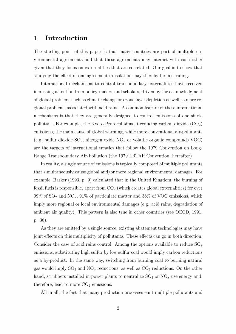
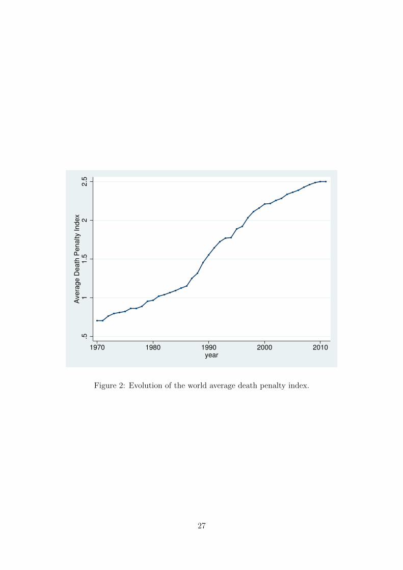
Moreover, the average death penalty index seems to vary significantly over time, as

shown by Figure 2. We also reject the null hypothesis of no variation through time

within a country as the F-statistic is F(38,5662)=88.69 (with a p-value of 0.00).




3 Results

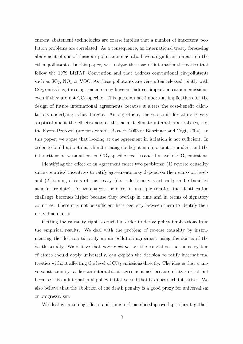
3.1 Individual agreements

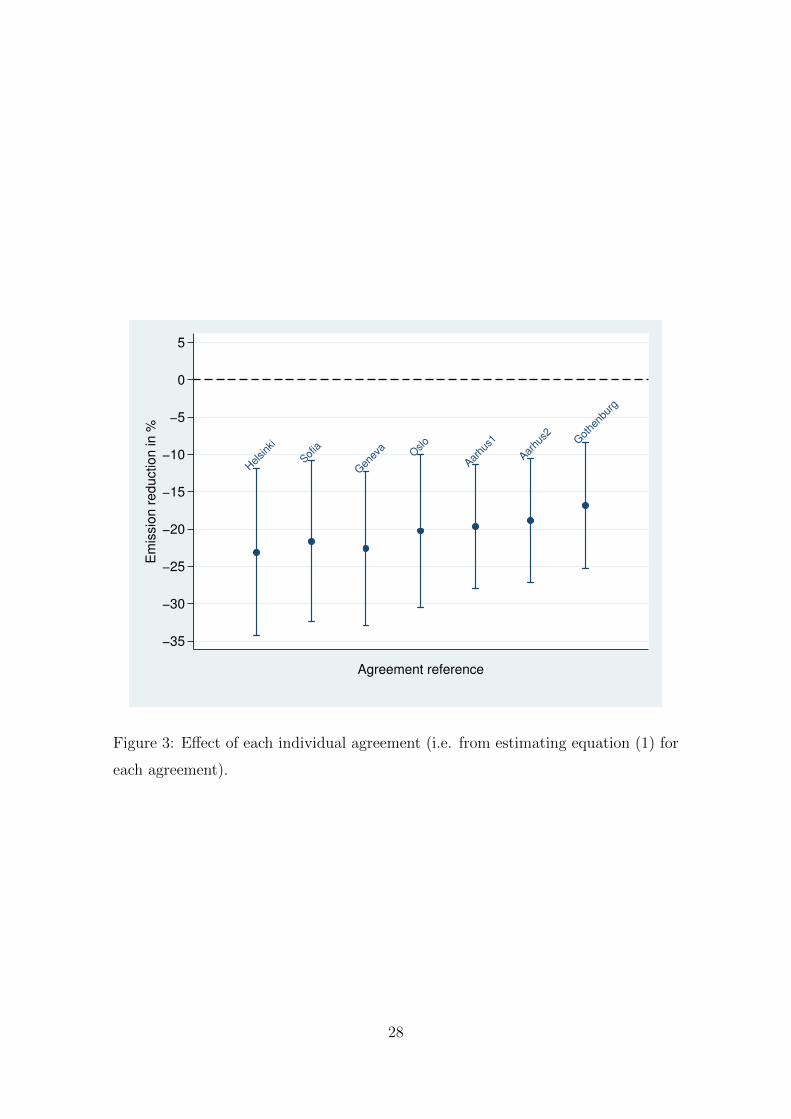
As an illustration, we first estimate equation (1) for each individual agreement k

(k = 1, ...7) in Table 1. We only present the results for the variables of interest Xkit−1

11Due to the lack of variations through time and across countries, we were not able to use

legalization of homosexual marriage or euthanasia as instruments.

14

in Figure 3.12 It appears that all the LRTAP treaties have a significant negative

impact on CO2 emissions. Furthermore, their effects are relatively similar. However,

it is not clear which effect we capture, due to the substantial overlap in terms of

membership and timing. This is why in the next section we turn to models in which

agreements are grouped into one variable that counts the number of agreements

ratified by each country, LRTAP .


3.2 Accumulation of treaties

Table 6 presents the results for the LRTAP variable of the various specifications

(equations (1)-(3)) detailed above. Equations (1) and (2) are estimated using a

standard panel two-way fixed effects estimator. To control for heteroskedasticity

and within country serial correlation, standard errors are estimated using the Huber-

White sandwich estimator, clustered at the country level. Results are shown in the

first two columns. The last three columns refer to equation (3). Columns 3 and 4

show the results for the Anderson-Hsiao estimator, while column 5 reports the results

for the Arellano-Bond estimator. In these last three columns, standard errors are

also clustered at the country level.


In column 1 of Table 6 (static specification), the ratification by one country of

each additional LRTAP agreement is associated with a reduction by approximately

4% of its CO2 emissions. When we turn to a dynamic model, results in column

2 suggest a strong inertia in CO2 emissions since the estimated coefficient of the

lagged dependent variable is ρ = 0.794. The effect of LRTAP agreements is still

negative and statistically significant. Note that this is a short term effect, i.e. the

effect after controlling for the response of the previous years.

As noted in the previous section, some econometric problems arise from estimat-

ing equation (2): CO2 emissions may be non-stationary and the lagged dependent

variable is correlated with the error term. We run some panel unit root tests. Re-

sults are shown in Table 7. For all the tests, we reject the null hypothesis of the

12Results for the control variables are very similar to those of models analyzed in the next section.

15

existence of unit roots in all panels. Our initial dynamic fixed-effect model would

thus be fine as the bias of the autoregressive term would be negligible given the

relative long time span of the data. However, when we run country-specific panel

unit root tests, we find that about 21% of panels contain a unit root.13 For this

reason, we turn to the model in first difference (equation (3)) estimated using the

Anderson-Hsiao estimator.


In column 3, we only instrument the lagged dependent variable in first difference

using lags 2 to 4 in level. In column 4, we deal with the problem of reverse causality

by assuming that treaties’ ratification may be endogenous and by instrumenting the

differenced LRTAP variable with the death penalty index in level. The coefficient

of LRTAP remains negative and significantly different from zero. To test for the

validity of our instruments, we look at the first-stage equations (see Table (8)) of

models in columns 3 and 4, which are given by:

∆yjit−1 = δt−δt−1+ψj1DPit−1+ψj

2log(CO2)it−2+ψj3log(CO2)it−3+ψj

4log(CO2)it−4+∆Zitθj+∆uit

(4)

For j = 1, 2; where y1it−1 = LRTAPit−1, y2it−1 = log(CO2)it−1 and DPit−1 is the

death penalty index.

From Table (8), death penalty seems to be a good determinant for the ratification

of LRTAP agreements.14 The strength of the instruments (the lagged dependent

variable in level and the status of the death penalty) is further checked with tests

presented in Table 9. Instruments are quite strong. Indeed, we are sure at 95% that

the maximal bias associated with the coefficient of interest is less than 10% of the

OLS bias (weak identification test).15 From the under-identification test, we can

conclude that the first-stage equation is identified, i.e. the excluded instruments

(Death Penalty and lags 2 and 4 of log(CO2)) are relevant (correlated with the

endogenous regressor).

13Results are not reported here but are available upon request.14Note that this result cannot be explained by an eventual common trend (i.e. the fact that

both LRTAP and DP increase monotonically) as we use the status of the death penalty in level to

instrument LRTAP in first-difference.15Even if the Cragg-Donald Wald F Statistics is much higher than the Kleibergen-Paap rank

Wald F statistic, the use of the Kleibergen-Paap statistic is more appropriate. It generalizes the

Cragg-Donald statistic to the case of non-i.i.d. errors, allowing for heteroskedasticity, autocorrela-

tion and/or cluster robust statistics.

16



The value obtained with the AH estimator when treaties’ ratification is also

instrumented (column 4), seems too high: each additional treaty ratified by one

country reduces the CO2 emissions in that country by approximately 10%. As men-

tioned earlier, given the small efficiency of the estimator, the coefficient of interest

may be very imprecisely estimated in column 4. The AB estimator in column 5

provides a more efficient estimator than AH and we will consider it as our final

result.

The effect of LRTAP is negative and significant at the level of 1%: ratification

of an additional treaty has a short term impact of 2.5% on CO2 emissions, i.e. after

controlling for the response of previous years. Obviously, the estimated coefficients

in the dynamic and static models are not directly comparable. However, in the dy-

namic specification, the cumulative effect of an agreement on CO2 emissions can be

computed as β/(1−ρ), where β = −0.025 is the short term coefficient and ρ = 0.707

is the coefficient of the lagged dependent variable. With our estimates, this cumula-

tive effect is thus equal to approximately 8.5% for LRTAP treaties, suggesting that

the effect estimated with the static specification (4%) was probably underestimated.

As this result may be sensitive to the choice of the point in time from which a

treaty has an impact on emissions, we have re-estimated the model using entry into

force rather than ratification. The results (not reported in full but available upon

request) are similar (and even stronger) compared to those in column 5 of Table

6: the short-term impact of LRTAP agreements is 6.02%, with t-value -2.72. Our

results thus seem robust to the definition of the variable of interest.

To the best of our knowledge, there do not exist tests of the strength of instru-

ments in AB models. We rely on the results of the first-stage AH estimator (Table

8) as is generally done in the literature. We also present the Arellano-Bond tests

for AR(1) and AR(2) (See Table 10), for which the null hypothesis is that there is

no autocorrelation in the error term. AR(1) is expected in first differences, because

the differenced error terms in t and t − 1 both contain the εit−1 term. To check if

our instruments in levels are good instruments for the first-difference, we need to

look at AR(2). Autocorrelation indicates that lags of the dependent variable (and

17

any other variables used as instruments), are in fact endogenous, thus bad instru-

ments. As shown in Table 10, we cannot reject that our instruments in level are

valid instrument.


A potential weakness of the AB estimator (and thus also AH estimator) is that

the lagged levels may be rather poor instruments for first differenced variables. This

is especially the case if the dependent variable is close to a unit root, which seems

not to be the case here since ρ = 0.707 (see column 5). In the presence of poor

instruments in level, one could use the augmented version – system GMM. The

system GMM estimator (Blundell and Bond) uses the level equation (e.g. equation

(2) in our case). The variables in levels in the second equation are instrumented with

their own first differences. However, using this method in a panel with fixed effects

requires a new assumption: the first-differenced variables used as instruments for the

variables in levels should not be correlated with the unobserved country effects αi in

equation (2). In our case, this would require, for example, that the first-differenced

death penalty index or GDP are not correlated with the fixed-effects capturing

unobserved heterogeneity among countries, which is too strong as an assumption.

Moreover, as the first-stage regression and the Stock and Yogo’s test show, our

instruments are not weak.

Finally, for the other results, most of the control variables have the expected

sign. A higher GDP level is associated with higher CO2 emissions. The coefficients

of trade openness and population are positive but not significant. Both the shares

of agricultural and industrial productions imply an increase of CO2 emissions, but

they do not have a significant impact. Democracy has a positive effect on CO2

emissions (but only significant at the 10% level). The GDP growth rate coefficient

has a negative sign in the static specification of column 1, but a positive sign in

the dynamic specifications (indicating increases in energy consumption that seem to

offset energy efficiency improvements during periods of economic growth).16

16Given that the dynamic model seems to be the appropriate specification for the process un-

derlying CO2 emissions, the coefficient estimated in the dynamic model seems more reliable.

18

4 Interpretation of the results

Results show that, even if they are not directly targeted towards CO2 emissions,

LRTAP treaties are still effective in reducing those emissions. In the light of the

definition of the independent variable used, i.e. the sum of ratified treaties, it

seems that the effects of the various agreements accumulate. By ratifying additional

agreements, countries might complete the initial one and control other sources of

emissions: each additional ratified agreement is associated with an annual reduction

of CO2 emissions of approximately 2.5%. Our result also suggests that if all countries

ratify an additional air-pollution treaty, the world CO2 emissions will be reduced by

2.5%, controlling for the response of previous year and by 8.5% in the long run.

We propose two interpretations for this result. First, pollutants covered by

LRTAP agreements (SO2, NOx or VOC) are more local pollutants than greenhouse

gases, such as CO2. Agreements on local pollutants are easier to reach because

they involve less countries and the environmental effects of these pollutants are

more visible. These more visible effects lead to a higher commitment by national

politicians. They are more willing to enforce the international agreement and they

accept to implement more ambitious targets.

Second, LRTAP agreements present a relatively effective design given the nature

of their objective. On the one hand, they are more focused than the Kyoto Protocol,

for example: each LRTAP treaty deals with only one air-pollutant (except the 1999

Gothenburg Protocol) while the Kyoto Protocol deals with different greenhouse

gases. On the other hand, LRTAP agreements have not only clear targets but well

identified means to meet these targets, whereas the Kyoto protocol has less clear

means to achieve them. For example, the annexes of these agreements include a

description of the measures available to reduce the pollutant covered by the treaty.

The relative ease in implementing these treaties means that they are effectively

implemented and are able to reduce CO2 as a byproduct.

5 Sensitivity Analysis

In this section, we test the robustness of our benchmark results, i.e. that the ratifica-

tion of each additional air-pollution treaty is associated with a significant reduction

19

of CO2 emissions. Details of these robustness checks can be found in appendix B.

They are summarized below.17

Other set of controls (see Table 12 in appendix B). Environmental agreements

might affect the composition of the industry or the level of imports/exports (our

measure of trade openness) and, as they are included as control variables, our results

may be biased. However, omitting these two control variables does not change the

main results (the size and the significativity of the results are even higher). Other

control variables (e.g. the amount of foreign direct investments or the proportion

of electricity production from natural gas sources, which is less sulfur and carbon

intensive than coal for example) were also introduced in the AB specification, but

this did not change the main results of the model (see columns 3 and 4). Other

variables would have been interesting to study, such as the legal origin (see Stern,

2012). However, these variables do not vary over time and are likely to be captured

by the fixed effects or to disappear when we turn to the AH or AB estimations.

Sub-samples of countries (see Tables 13 and 14 in appendix B). We test

whether our benchmark results are not driven by a particular sub-sample of coun-

tries. The thrust of our argument continues to hold. Air-pollution agreements have

a negative impact on CO2 emissions, whatever the sub-sample considered: poor or

rich countries (in terms of GDP per capita), without EU15, without BRIC countries

(i.e. Brazil, China, India and Russia) or without economies in transition (EiTs).18

Net CO2 emissions (see Table 13 in appendix B). Our data on CO2 emissions

do not take into account emissions/removals from land use, land use change and

forestry (LULUCF). The data used in this paper are thus gross CO2 emissions.

17Additionally, we have reduced our sample by limiting the number of years in two different

ways: (i) we have only considered every five years to break any possible auto-correlation in the

error term and (ii) we have only considered recent years (i.e. after 1980 and after 1985). Results

are not presented here but they remain unchanged.18BRIC countries (except Russia) have experienced a very strong economic growth and increase

in their CO2 emissions in the last decades and they did not ratify many agreements related to

air-pollution. By contrast, the reduction of emissions observed in EiTs countries in the 1990s is

mainly due to the economic collapse in those former Soviet States. It can then be argued that

the success of air-pollution agreements in reducing CO2 emissions is an artifact of those transition

countries’ industrial restructuring.

20

However, there are examples of countries, such as Russia, that have reduced their

gross CO2 emissions and at the same time have destroyed substantial parts of their

forest area, thereby increasing their net CO2 emissions. In this case, emission reduc-

tions are over-estimated in the basic model since the destruction of forests, which

are carbon sinks, increases the stock of CO2 in the atmosphere. In order to get

an idea of the effect of air-pollution agreements on net CO2 emissions, we split our

sample into two groups: countries that are not concerned by this problem of mas-

sive deforestation and those concerned by deforestation (information comes from

http://www.grida.no). In countries not concerned by deforestation, the gross CO2

emissions (our data) should be very similar to net emissions and the coefficient of

the variable of interest for those countries (column 4) should thus not be affected

by the fact that we do not take into account removals from LULUCF.

6 Conclusion

The objective of this paper is to test for the effectivity of air-pollution agreements on

the level of CO2 emissions. There is strong evidence that CO2 (a global pollutant) is

often released with more conventional air-pollutants. Pollution abatements imposed

by international treaties targeted to these conventional pollutants may thus jointly

reduce the flows of both types of pollutants. Our analysis focuses on the effects of

the treaties that follow the 1979 LRTAP Convention.

We deal with different issues pertaining to the identification of the effect of

these multiple agreements: (1) reverse causality, (2) timing effects and (3) time and

membership overlap between treaties. The main result is that LRTAP agreements,

even if they are not CO2-specific, have a statistically significant negative impact

on CO2 emissions. This puts forward the limitation of studying the effects of an

environmental agreement in isolation.

We suggest two possible explanations: first, the methods to implement emission

reduction targets foreseen in LRTAP agreements are well-identified in the treaties’

texts, which is not the case for the Kyoto Protocol. Second, air-pollutants causing

acid rains (e.g. SO2 or NOx) are more local pollutants than CO2. This highlights the

fact that the existence of an agreement is not sufficient. The nature of the agreement

21

and its content matter for its effectiveness in reducing polluting emissions.

This paper is a first attempt to study the ancillary effects of multiple air-pollution

treaties empirically in the context of climate change. However, climate change is

a very complex problem and this study can be extended in several ways to take

this complexity better into account. Among others, sulphur dioxide emissions are

turned into sulphate aerosols, which have only a short life time in the atmosphere,

but have a substantial cooling effect and can thus postpone the impact of climate

change (see Tol, 2004). SO2 reductions due to LRTAP treaties may thus partially

offset carbon emission reductions. This example shows that in order to design

an optimal international climate policy, it is crucial to understand and estimate

all the interactions between air-pollution and climate treaties and their respective

outcomes.

22

Tab

le1:

Inte

rnat

ional

Envir

onm

enta

lA

gree

men

tsre

late

dto

air-

pol

luti

on(M

itch

ell,

2002

-201

2)

Ref

.A

gree

men

tT

itle

and

sign

atu

red

ate

Rat

ifica

tion

Mem

ber

sa

star

tsin

Sta

rtin

gY

ear

2008

1P

roto

col

On

The

Red

uct

ion

Of

Su

lphu

rE

mis

sion

sO

r

1985

121

Th

eir

Tra

nsb

oun

dar

yF

luxes

By

At

Lea

st30

Per

Cen

t

(Hel

sin

ki,

1985

)

2P

roto

col

Con

cern

ing

The

Con

trol

Of

Em

issi

ons

of

1988

829

Nit

roge

nO

xid

esO

rT

hei

rT

ran

sbou

nd

ary

Flu

xes

(Sofi

a,19

88)

3P

roto

col

Con

cern

ing

The

Con

trol

Of

Em

issi

ons

Of

Vol

atil

e

1993

319

Org

anic

Com

pou

nd

sO

rT

hei

rT

ran

sbou

nd

ary

Flu

xes

(Gen

eva,

1991

)

4P

roto

col

On

Fu

rth

erR

edu

ctio

nO

fS

ulp

hu

rE

mis

sion

s(O

slo,

1994

)19

953

23

5P

roto

col

On

Hea

vy

Met

als

To

Th

eC

onve

nti

onO

nL

ong-

1998

124

Ran

geT

ran

sbou

nd

ary

air-

pol

luti

on(A

arhu

s,19

98)

6P

roto

col

On

Per

sist

ent

Org

anic

Pol

luta

nts

To

Th

e19

981

23

Con

venti

onO

nL

ong-

Ran

geT

ran

sbou

nd

ary

air-

pol

luti

on(A

arhu

s,19

98)

7P

roto

col

To

Ab

ate

Aci

difi

cati

on,

Eu

trop

hic

atio

nA

nd

Gro

un

d-L

evel

2002

322

Ozo

ne

To

Th

eC

onve

nti

onO

nL

RT

AP

(Got

hen

bu

rg,

1999

)

a.Mem

bersare

countriesth

atratify

oneparticulartrea

ty,eith

erin

thestartingyea

r(see

column3)orin

2008.

23

ChinaGerm

any

UnitedStates

01

23

45

67

8

Nu

mb

er

of

ratified

ag

ree

me

nts

0 20000 40000 60000

1980

China

Germany

UnitedStates

01

23

45

67

8

0 20000 40000 60000

1995

China

Germany

UnitedStates

01

23

45

67

8

0 20000 40000 60000

2008

GDP per capita

Figure 1: Ratification of LRTAP treaties and total CO2 emissions (in kilotons) as

functions of GDP per capita (in 2000 US dollars).

24

Tab

le2:

Cor

rela

tion

mat

rix

for

the

year

2008

1985

1988

1991

1994

1998

1998

1999

Hel

sinki

Sofi

aG

enev

aO

slo

Aar

hus

(1)

Aar

hus

(2)

Got

hen

burg

1985

Hel

sinki

1

1988

Sofi

a0.

8242

1

1991

Gen

eva

0.77

060.

7779

1

1994

Osl

o0.

6815

0.86

930.

8393

1

1998

Aar

hus

(1)

0.66

240.

7533

0.76

330.

7732

1

1998

Aar

hus

(2)

0.68

150.

7287

0.78

360.

7946

0.92

461

1999

Got

hen

burg

0.53

870.

7037

0.74

860.

7650

0.84

710.

7650

1

25

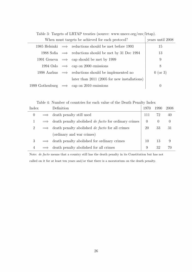
Table 3: Targets of LRTAP treaties (source: www.unece.org/env/lrtap).

When must targets be achieved for each protocol? years until 2008

1985 Helsinki =⇒ reductions should be met before 1993 15

1988 Sofia =⇒ reductions should be met by 31 Dec 1994 13

1991 Geneva =⇒ cap should be met by 1999 9

1994 Oslo =⇒ cap on 2000 emissions 8

1998 Aarhus =⇒ reductions should be implemented no 0 (or 3)

later than 2011 (2005 for new installations)

1999 Gothenburg =⇒ cap on 2010 emissions 0

Table 4: Number of countries for each value of the Death Penalty Index

Index Definition 1970 1990 2008

0 =⇒ death penalty still used 111 72 40

1 =⇒ death penalty abolished de facto for ordinary crimes 0 0 0

2 =⇒ death penalty abolished de facto for all crimes 20 33 31

(ordinary and war crimes)

3 =⇒ death penalty abolished for ordinary crimes 10 13 9

4 =⇒ death penalty abolished for all crimes 9 32 70

Note: de facto means that a country still has the death penalty in its Constitution but has not

called on it for at least ten years and/or that there is a moratorium on the death penalty.

26

.51

1.5

22.5

Avera

ge D

eath

Penalty Index

1970 1980 1990 2000 2010year

Figure 2: Evolution of the world average death penalty index.

27

Helsink

i

Sofia

Gen

eva

Oslo

Aarhu

s1

Aarhu

s2 Got

henb

urg

−35

−30

−25

−20

−15

−10

−5

0

5

Em

issio

n r

eduction in %

Agreement reference

Figure 3: Effect of each individual agreement (i.e. from estimating equation (1) for

each agreement).

28

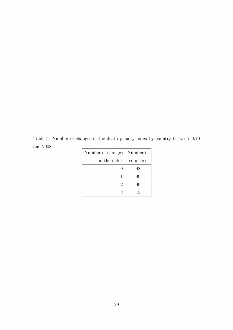
Table 5: Number of changes in the death penalty index by country between 1970

and 2008.

Number of changes Number of

in the index countries

0 48

1 49

2 40

3 13

29

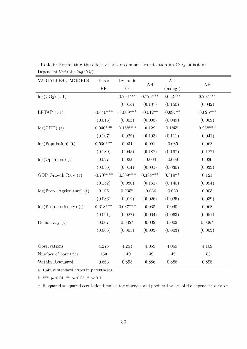
Table 6: Estimating the effect of an agreement’s ratification on CO2 emissions.

Dependent Variable: log(CO2)

VARIABLES / MODELS Basic DynamicAH

AHAB

FE FE (endog.)

log(CO2) (t-1) 0.794*** 0.775*** 0.692*** 0.707***

(0.016) (0.137) (0.150) (0.042)

LRTAP (t-1) -0.040*** -0.009*** -0.012** -0.097** -0.025***

(0.013) (0.002) (0.005) (0.049) (0.009)

log(GDP) (t) 0.940*** 0.188*** 0.129 0.185* 0.258***

(0.107) (0.029) (0.103) (0.111) (0.041)

log(Population) (t) 0.536*** 0.034 0.091 -0.085 0.068

(0.189) (0.045) (0.182) (0.197) (0.127)

log(Openness) (t) 0.027 0.023 -0.004 -0.009 0.036

(0.056) (0.014) (0.031) (0.030) (0.033)

GDP Growth Rate (t) -0.707*** 0.309*** 0.388*** 0.319** 0.121

(0.152) (0.080) (0.131) (0.140) (0.094)

log(Prop. Agriculture) (t) 0.105 0.035* -0.036 -0.039 0.003

(0.086) (0.019) (0.026) (0.025) (0.039)

log(Prop. Industry) (t) 0.318*** 0.087*** 0.035 0.040 0.068

(0.091) (0.022) (0.064) (0.063) (0.051)

Democracy (t) 0.007 0.002* 0.002 0.002 0.006*

(0.005) (0.001) (0.003) (0.003) (0.003)

Observations 4,275 4,253 4,059 4,059 4,109

Number of countries 150 149 149 149 150

Within R-squared 0.663 0.898 0.886 0.886 0.898

a. Robust standard errors in parentheses.

b. *** p<0.01, ** p<0.05, * p<0.1.

c. R-squared = squared correlation between the observed and predicted values of the dependent variable.

30

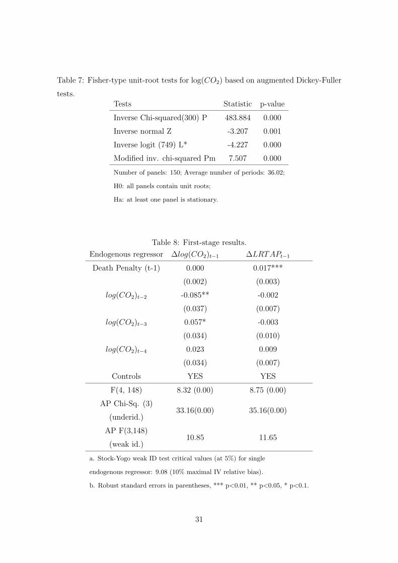
Table 7: Fisher-type unit-root tests for log(CO2) based on augmented Dickey-Fuller

tests.

Tests Statistic p-value

Inverse Chi-squared(300) P 483.884 0.000

Inverse normal Z -3.207 0.001

Inverse logit (749) L* -4.227 0.000

Modified inv. chi-squared Pm 7.507 0.000

Number of panels: 150; Average number of periods: 36.02;

H0: all panels contain unit roots;

Ha: at least one panel is stationary.

Table 8: First-stage results.

Endogenous regressor ∆log(CO2)t−1 ∆LRTAPt−1

Death Penalty (t-1) 0.000 0.017***

(0.002) (0.003)

log(CO2)t−2 -0.085** -0.002

(0.037) (0.007)

log(CO2)t−3 0.057* -0.003

(0.034) (0.010)

log(CO2)t−4 0.023 0.009

(0.034) (0.007)

Controls YES YES

F(4, 148) 8.32 (0.00) 8.75 (0.00)

AP Chi-Sq. (3)33.16(0.00) 35.16(0.00)

(underid.)

AP F(3,148)10.85 11.65

(weak id.)

a. Stock-Yogo weak ID test critical values (at 5%) for single

endogenous regressor: 9.08 (10% maximal IV relative bias).

b. Robust standard errors in parentheses, *** p<0.01, ** p<0.05, * p<0.1.

31

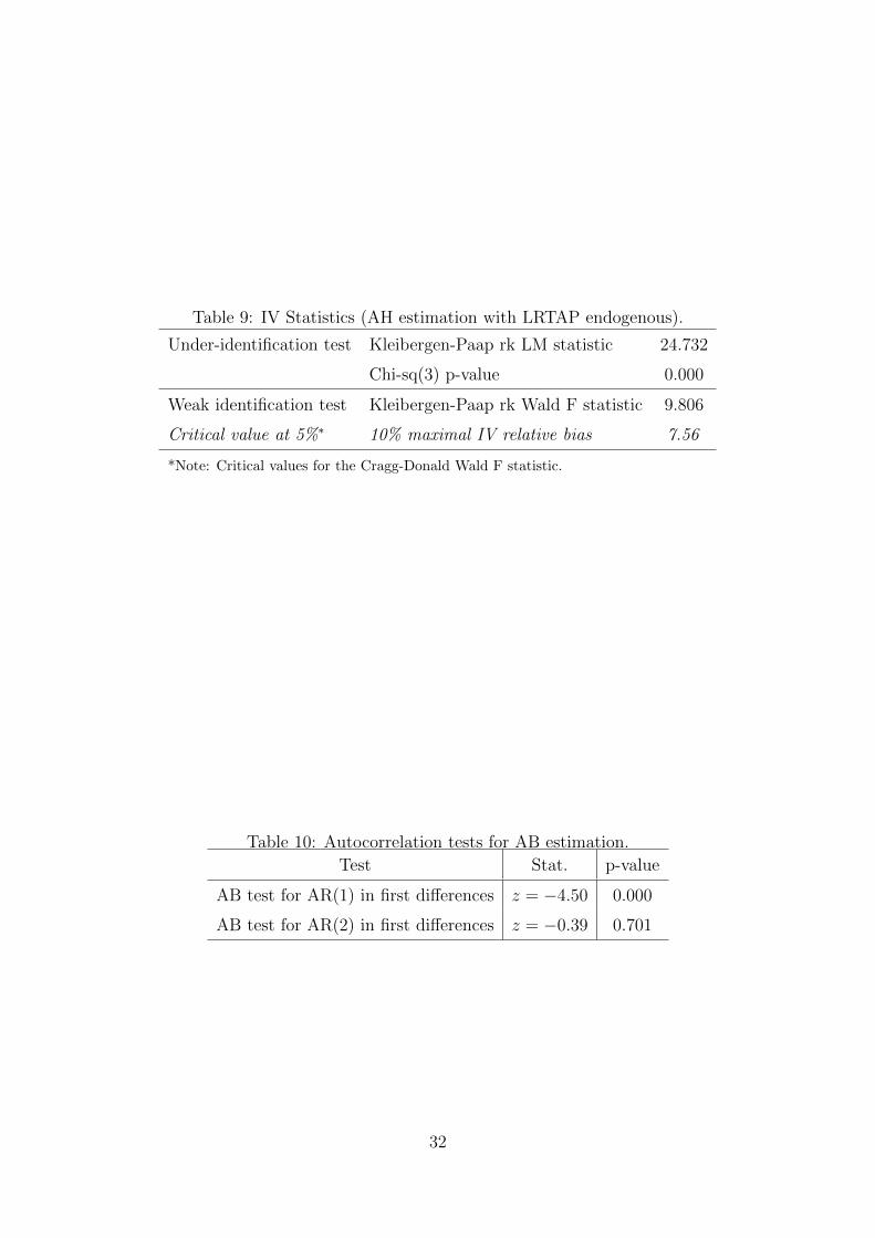
Table 9: IV Statistics (AH estimation with LRTAP endogenous).

Under-identification test Kleibergen-Paap rk LM statistic 24.732

Chi-sq(3) p-value 0.000

Weak identification test Kleibergen-Paap rk Wald F statistic 9.806

Critical value at 5%∗ 10% maximal IV relative bias 7.56

*Note: Critical values for the Cragg-Donald Wald F statistic.

Table 10: Autocorrelation tests for AB estimation.

Test Stat. p-value

AB test for AR(1) in first differences z = −4.50 0.000

AB test for AR(2) in first differences z = −0.39 0.701

32

Appendices

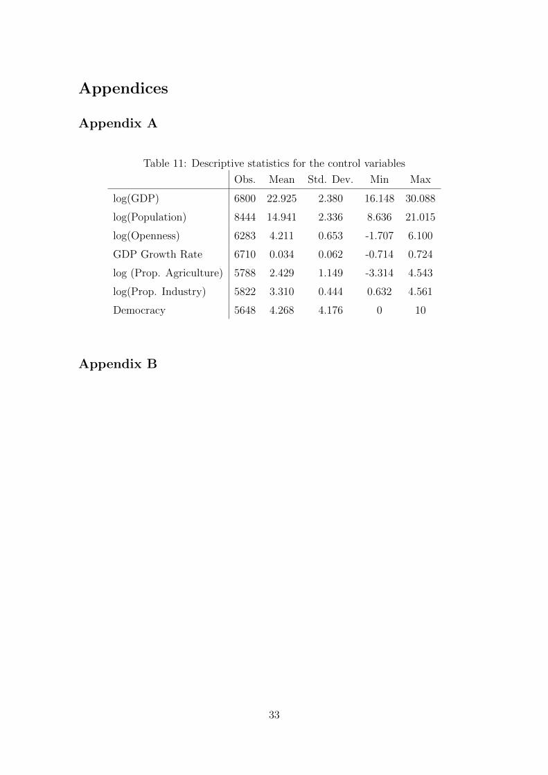
Appendix A

Table 11: Descriptive statistics for the control variables

Obs. Mean Std. Dev. Min Max

log(GDP) 6800 22.925 2.380 16.148 30.088

log(Population) 8444 14.941 2.336 8.636 21.015

log(Openness) 6283 4.211 0.653 -1.707 6.100

GDP Growth Rate 6710 0.034 0.062 -0.714 0.724

log (Prop. Agriculture) 5788 2.429 1.149 -3.314 4.543

log(Prop. Industry) 5822 3.310 0.444 0.632 4.561

Democracy 5648 4.268 4.176 0 10

Appendix B

33

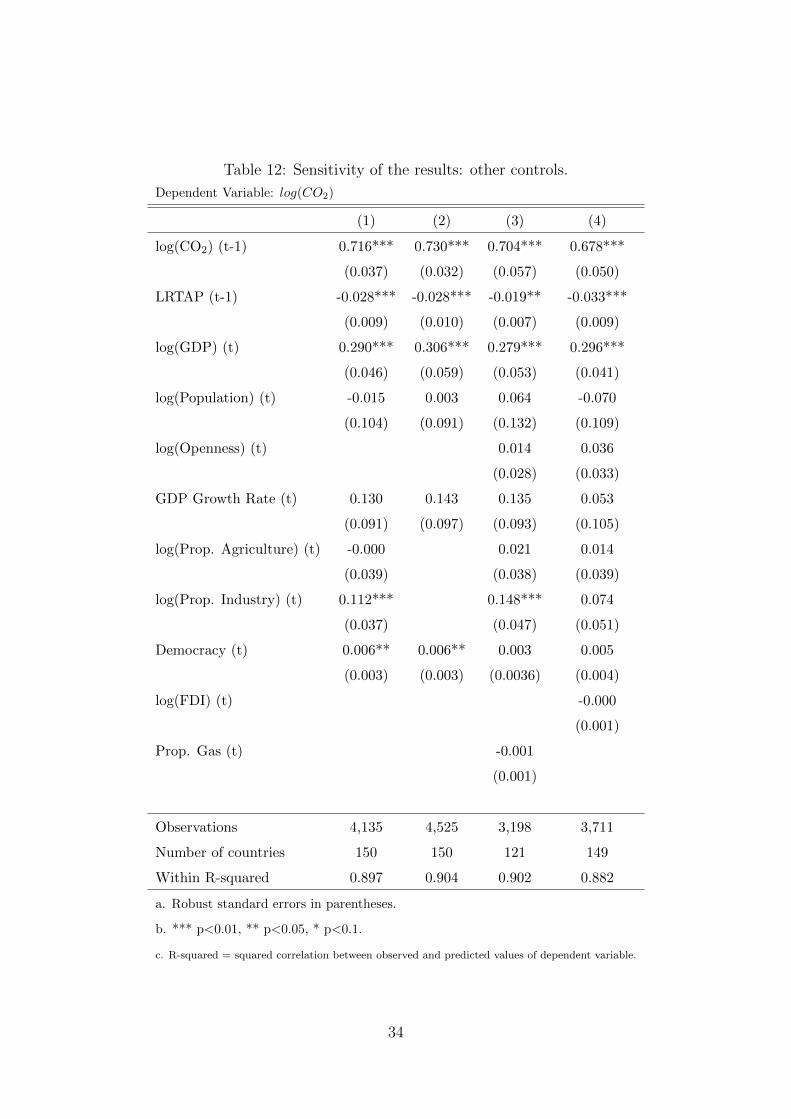
Table 12: Sensitivity of the results: other controls.


(1) (2) (3) (4)

log(CO2) (t-1) 0.716*** 0.730*** 0.704*** 0.678***

(0.037) (0.032) (0.057) (0.050)

LRTAP (t-1) -0.028*** -0.028*** -0.019** -0.033***

(0.009) (0.010) (0.007) (0.009)

log(GDP) (t) 0.290*** 0.306*** 0.279*** 0.296***

(0.046) (0.059) (0.053) (0.041)

log(Population) (t) -0.015 0.003 0.064 -0.070

(0.104) (0.091) (0.132) (0.109)

log(Openness) (t) 0.014 0.036

(0.028) (0.033)

GDP Growth Rate (t) 0.130 0.143 0.135 0.053

(0.091) (0.097) (0.093) (0.105)

log(Prop. Agriculture) (t) -0.000 0.021 0.014

(0.039) (0.038) (0.039)

log(Prop. Industry) (t) 0.112*** 0.148*** 0.074

(0.037) (0.047) (0.051)

Democracy (t) 0.006** 0.006** 0.003 0.005

(0.003) (0.003) (0.0036) (0.004)

log(FDI) (t) -0.000

(0.001)

Prop. Gas (t) -0.001

(0.001)

Observations 4,135 4,525 3,198 3,711

Number of countries 150 150 121 149

Within R-squared 0.897 0.904 0.902 0.882


b. *** p<0.01, ** p<0.05, * p<0.1.

c. R-squared = squared correlation between observed and predicted values of dependent variable.

34

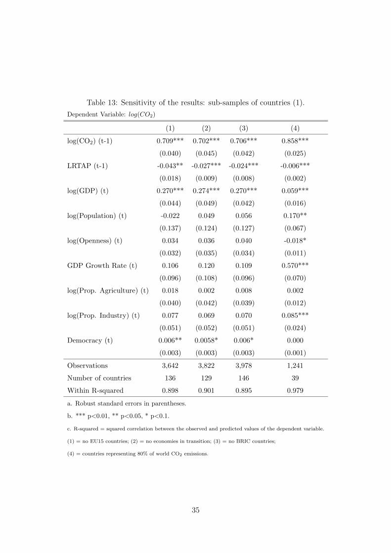
Table 13: Sensitivity of the results: sub-samples of countries (1).


(1) (2) (3) (4)

log(CO2) (t-1) 0.709*** 0.702*** 0.706*** 0.858***

(0.040) (0.045) (0.042) (0.025)

LRTAP (t-1) -0.043** -0.027*** -0.024*** -0.006***

(0.018) (0.009) (0.008) (0.002)

log(GDP) (t) 0.270*** 0.274*** 0.270*** 0.059***

(0.044) (0.049) (0.042) (0.016)

log(Population) (t) -0.022 0.049 0.056 0.170**

(0.137) (0.124) (0.127) (0.067)

log(Openness) (t) 0.034 0.036 0.040 -0.018*

(0.032) (0.035) (0.034) (0.011)

GDP Growth Rate (t) 0.106 0.120 0.109 0.570***

(0.096) (0.108) (0.096) (0.070)

log(Prop. Agriculture) (t) 0.018 0.002 0.008 0.002

(0.040) (0.042) (0.039) (0.012)

log(Prop. Industry) (t) 0.077 0.069 0.070 0.085***

(0.051) (0.052) (0.051) (0.024)

Democracy (t) 0.006** 0.0058* 0.006* 0.000

(0.003) (0.003) (0.003) (0.001)

Observations 3,642 3,822 3,978 1,241


Within R-squared 0.898 0.901 0.895 0.979


b. *** p<0.01, ** p<0.05, * p<0.1.


(1) = no EU15 countries; (2) = no economies in transition; (3) = no BRIC countries;

(4) = countries representing 80% of world CO2 emissions.

35

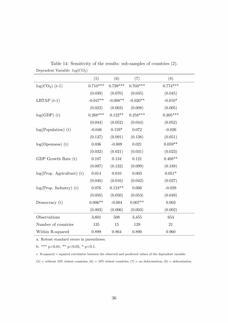
Table 14: Sensitivity of the results: sub-samples of countries (2).


(5) (6) (7) (8)

log(CO2) (t-1) 0.710*** 0.739*** 0.703*** 0.774***

(0.039) (0.070) (0.045) (0.045)

LRTAP (t-1) -0.047** -0.008** -0.020** -0.010*

(0.022) (0.003) (0.008) (0.005)

log(GDP) (t) 0.268*** 0.122** 0.258*** 0.305***

(0.044) (0.052) (0.044) (0.052)

log(Population) (t) -0.046 0.159* 0.072 -0.026

(0.137) (0.091) (0.138) (0.051)

log(Openness) (t) 0.036 -0.009 0.021 0.059**

(0.032) (0.021) (0.031) (0.023)

GDP Growth Rate (t) 0.107 0.134 0.121 0.408**

(0.097) (0.132) (0.099) (0.188)

log(Prop. Agriculture) (t) 0.014 0.010 0.003 0.051*

(0.040) (0.016) (0.042) (0.027)

log(Prop. Industry) (t) 0.076 0.124** 0.066 -0.029

(0.050) (0.050) (0.053) (0.049)

Democracy (t) 0.006** -0.004 0.007** 0.003

(0.003) (0.006) (0.003) (0.002)

Observations 3,601 508 3,455 654


Within R-squared 0.899 0.864 0.890 0.960


b. *** p<0.01, ** p<0.05, * p<0.1.


(5) = without 10% richest countries; (6) = 10% richest countries; (7) = no deforestation; (8) = deforestation.

36

Acknowledgments : This research has received funding from the FRS-FNRS and

the ERC grant MaDEM. We thank Estelle Cantillon, Gregoire Garsous and Mar-

jorie Gassner for their very helpful comments. We are also indebted to the CRED

Workshop participants, in particular Jean-Marie Baland. We are grateful to Paola

Conconi, Andreas Lange, Patrick Legros and David Martimort for their comments.

References

[1] Aakvik, A., Tjøtta, S., 2011. Do collective actions clear common air? The effect

of international environmental protocols on sulphur emissions. European Journal

of Political Economy 27 (2), 343-351.

[2] Aichele, R., Felbermayr, G., 2012. Kyoto and the carbon footprint of nations.

Journal of Environmental Economics and Management, 63 (3), 336-354.

[3] Ambec, S., and J. Coria, 2013. Prices vs quantities with multiple pollutants,

Journal of Environmental Economics and Management, 66, 123-140.

[4] Arellano, M., and Bond, S. (1991). Some tests of specification for panel data:

Monte Carlo evidence and an application to employment, Review of Economic

studies, 58, 277-297.

[5] Barker, T. , 1993. Ancillary benefits of greenhouse gas abatement: The effects of

a UK carbon/energy tax on air pollution, Discussion Paper No. 4, Department

of Applied Economics, University of Cambridge, UK.

[6] Barrett, S., 2003. Environment and Statecraft: The Strategy of Environmental

Treaty-making. Oxford University Press, Oxford.

[7] Bohringer, C., Vogt, C., 2004. The dismantling of a breakthrough: the Kyoto

Protocol as symbolic policy. European Journal of Political Economy 20 (3), 597-

617.

[8] Bollen, J., B. van der Zwaan, C. Brink, H. Eerens, 2009. Local air pollution and

global climate change: A combined cost-benefit analysis, Resource and Energy

Economics, 31, 161-181.

37

[9] Bratberg, E., Tjøtta, S., Øines, T., 2005. Do voluntary international environmen-

tal agreements work?. Journal of Environmental Economics and Management 50

(3), 583-597.

[10] Burtraw, D., A. Krupnick, K. Palmer, A. Paul, M. Toman, and C. Bloyd, 2001.

Ancillary Benefits of Reduced Air Pollution in the United States from Moderate

Greenhouse Gas Mitigation Policies in the Electricity Sector, Discussion Paper

0161, Resources for the Future.

[11] Caplan, A. J., and E. C. D. Silva, 2005. An efficient mechanism to control

correlated externalities: redistributive transfers and the coexistence of regional

and global pollution permit markets, Journal of Environmental Economics and

Management, 49, 68-82.

[12] Cole, M. A., 2004. Trade, the Pollution Haven Hypothesis and the Environ-

mental Kuznets Curve: Examining the Linkages. Ecological Economics 48 (1),

71-81.

[13] Congleton, R.D., 1992. Political Institutions and pollution control. Review of

Economics and Statistics 74 (3), 412-421.

[14] Copeland, B.R., Taylor, M.S., 2004. Trade, growth and the environment. Jour-

nal of Economic Literature 42 (1), 7-71.

[15] Egger, P., Wamser, G., 2013. Multiple Faces of Preferential Market Access:

Their Causes and Consequences. Economic Policy 28(73), 143-187.

[16] Friedl, B., Getzner, M., 2003. Determinants of CO2 emissions in a small open

economy. Ecological Economics 45 (1), 133-148.

[17] Galeotti,M., Lanza, A., Pauli, F., 2006. Reassessing the environmental Kuznets

curve for CO2 emissions: A robustness exercise. Ecological Economics 57 (1),

152-163.

[18] Greenberg, D. F., and V. West, 2008. Siting the Death Penalty Internationally,

Law & Social Inquiry, 33 (2), 295-343.

38

[19] International Energy Agency (2010), CO2 Emissions from Fuel Combustion.

Highlights, from http://www.iea.org/co2highlights/.

[20] Li, Q., Reuveny, R., 2006. Democracy and Environmental Degradation. Inter-

national Studies Quarterly 50 (1), 935-956.

[21] Mitchell, R. B., 2002-2012. International Environmental Agreements Database

Project (Version 2012.1), Available at: http://iea.uoregon.edu/.

[22] Mitchell, R.B., 2003. International Environmental Agreements: A Survey of

Their Features, Formation, and Effects. Annual Review of Environment and

Resource 28, 429-461.

[23] Murdoch, J. C., Sandler, T., 1997. The voluntary provision of a pure public

good: the case of reduced CFC emissions and the Montreal Protocol. Journal of

Public Economics 63 (3), 331-349.

[24] Neumayer, E., 2008. Death Penalty: The Political Foundations of the Global

Trend toward Abolition. Human Rights Review, 9(2), 241-268.

[25] OECD (Organisation for Economic Cooperation and Development), 1991. The

State of the Environment. OECD, Paris.

[26] Panayotou, T., 1997. Demystifying the Environmental Kuznets Curve: Turning

a Black Box into a Policy Tool. Environment and Development Economics 2 (4),

465-484.

[27] Shi, A., 2002. The Impact of Population Pressure in Global Carbon Dioxide

Emissions, 1975-1996: Evidence from Pooled Cross-Country Data. Ecological

Economics 44 (1), 29-42.

[28] Stern, D. I., 2002. Explaining Changes in Global Sulfur Emissions: an Econo-

metric decomposition approach. Ecological Economics 42 (1-2), 201-220.

[29] Stern, N., 2006. Stern Review: The economics of Climate

Change. Report to the UK Prime Minister and Chancellor, London

(http://webarchive.nationalarchives.gov.uk).

39

[30] Stern, D. I., 2012. Modeling international trends in energy efficiency, Energy

Economics, 34, 2200-2208.

[31] Tol, R.S.J., 2004. Multi-gas emission reduction for climate change policy: an

application of FUND. Energy Journal, Volume Multi-Greenhouse Gas Mitigation

and Climate Policy, Special Issue 3, 235-250

[32] van Vuuren, D. P., Riahi, K., 2008. Do recent emission trends imply higher

emissions forever?. Climatic Change 91 (3-4), 237-248.

40

measuring the impact of multiple air-pollution agreements

Documents