measuring the fiscal - unt

Measuring the Fiscal "Blood Pressure" of the States - 1964-1975

An Information Paper

Advisory Commission on Intergovernmental Relations Washington, D. C. 20575

February 1977

M-111

efac

T he Commission has a continuing interest in the fiscal integrity of state and local because i t is a necessary characteristic of a well balanced federal system. In 1962, the Commission published Measures of State and Local Fiscal Capac- ity and Tax Effort. This information report developed estimates of the fiscal capacity for each of the 50 state-local systems assuming average use of the various tax sources - the "representative tax system" approach. In 1971, the Commission is- sued a second information report using a revised and expanded concept of the representative financing system that encompassed both tax and non-tax revenue - Measuring the Fiscal Capacity and Effort of State and Local Areas.

In this information report, the concept of fiscal stress is developed measuring tax effort not merely at a single point in time but over the recent iii

past. At best, these fiscal pressure findings should be

viewed as but one of the aids to help policymakers balance the benefits and burdens that flow from changing the relationship between their public and private economies. For example, some states with high fiscal pressure readings may want to reduce the growth rate of the public sector and stimulate private development. On the other hand, some states may decide that the continuation of above average tax burdens constitutes sound public policy. The same difference of opin- ion will be apparent at the other end of the fiscal stress spectrum. Some states with low fiscal pressure readings may use this evidence as an argument for strengthening the public sector. In sharp contrast, policymakers in other low pressure states may cite these findings as support for their belief that a continuation of conservative fiscal policies is necessary to maintain a favorable com- petitive position.

Some would interpret the growing disparities in interstate fiscal pressure as a justification for re- medial federal action. For this reason, the authors have examined the pros and the cons of alternative federal strategies.

The policy alternatives set forth in this report have not been reviewed by the Commission and this document, therefore, should be considered as an information report only.

Robert E . Merriam Chairman

Acknowledgments

ohn Ross, senior academic resident in public J finance, and John Shannon, assistant director of the taxation and public finance staff, coauthored this study. Gordon Folkman and Richard Reeder of the Commission staff assisted with the data gathering and calculations. The authors received useful comments on an early draft of the study from public finance scholars and teachers, tax ad- ministrators, and tax practitioners.

This report was originally presented as a paper at the Conference on State and Local Finance at the University of Oklahoma on October 15, 1976, and is planned to be published as a part of the conference proceedings - Policies and Practices in State and Local Financing - edited by Professor Walter E. Scheffer. This report is being reprinted by ACIR for the convenience of those who will not have ready access to the conference proceedings.

The full responsibility for content and accuracy rest, as always, with the Advisory Commission on Intergovernmental Relations staff.

Wayne F . Anderson Executive Director

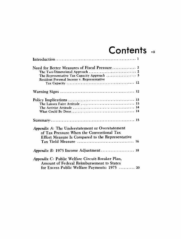
Contents vii

................................................... Introduction 1

............... Need for Better Measures of Fiscal Pressure 2 .............................. The Two-Dimensional Approach 2

................... The Representative Tax Capacity Approach 3 Resident Personal Income v . Representative

........................................... Tax Capacity 12

............................................... Warning Signs 12

.......................................... Policy Implications 13 .................................. The Laissez Faire Attitude 13

....................................... The Activist Attitude 14 ........................................ What Could Be Done 14

Appendix A: The Understatement or Overstatement of Tax Pressure When the Conventional Tax Effort Measure Is Compared to the Representative

.................................... Tax Yield Measure 16

..................... Appendix B: 1975 Income Adjustment 18

Appendix C: Public Welfare Circuit-Breaker Plan. Amount of Federal Reimbursement to States for Excess Public Welfare Payments: 1975 .......... 20

Tables

viii

1. A Two-Dimensional Measure of Relative State-Local Fiscal Pressure Using Resident Personal Income to Estimate Fiscal Capacity: 1964-75 . . . . . . . . . . . . . . . . . . . . . . . . . . . . . 4

2. A Two-Dimensional Measure of Relative State-Local Fiscal Pressure Using Resident Personal Income to Estimate Fiscal Capacity: Dividing the States into

. . . . . . . . . . . . . . . . . . . . . . . . . . . . . . . . . . . . . . . . . . . Quadrants: 1964-75 6

3. A Two-Dimensional Measure of Relative State-Local Fiscal Pressure Using the Representative Tax

. . . . . . . . . . . . . . . . . . Method to Estimate Fiscal Capacity: 1964-75 8

4. A Two-Dimensional Measure of Relative State-Local Fiscal Pressure Using the Representative Tax Method to Estimate Fiscal Capacity: Dividing the States

. . . . . . . . . . . . . . . . . . . . . . . . . . . . . . . . . . . . . into Quadrants: 1964-75 10

Appendix A: The Understatement or Overstatement of Tax Pressure When the Conventional Tax Effort Measure Is Compared to the Representative Tax Yield Measure . . . . . . . . . . . 16

............................ Appendix B: 1975 Income Adjustment 19

Appendix C : Public Welfare Circuit-Breaker Plan, Amount of Federal Reimbursement to States for Excess Public

. . . . . . . . . . . . . . . . . . . . . . . . . . . . . . . . . . . . . . Welfare Payments: 1975 20

Charts 1. A Two-Dimensional Measure of Relative State-Local

Fiscal Pressure Using Resident Personal Income to Estimate Fiscal Capacity: State-Local Systems More Than

. . . . . . . . . . . . . . . . . . . . . One Standard Deviation from the Median . 7

2. A Two-Dimensional Measure of Relative State-Local Fiscal Pressure Using the Representative Tax Method to Estimate Fiscal Capacity: State-Local Systems More

. . . . . . . . . . . . . . . . Than One Standard Deviation from the Median 11

Measuring the Fiscal "Blood Pressure"

of the States: 1 964- 1 975

D INTRODUCTION isparities in economic growth rates among

various regions of the nation have become sufficiently severe to attract the attention of the popular press. Business Week, in its May 17, 1976, issue, actually announced the coming of the "second war between the states"' as a result of the rapid shift of population, capital, and jobs from the Northeast and Midwest to the South and the West. Following this theme, the National Journal recently published a study of regional differences in federal spending patterns. The study con- cluded that "federal tax and spending policies are causing a massive flow of wealth from the North- east and Midwest to the fast growing Southern and Western regions of the n a t i ~ n , " ~ thus exacerbating present growth patterns. It goes on to add:

The states at the receiving end of high federal outlays (those in the South and West) also tend to be those that tax their own citizens least for state and local government services.

On the other hand, the balance of payments situation generally is adverse in the Northeast and Midwest, where population is stagnant or

"'The Second War Between the States," Business Week, May 17, 1976, No. 2432, pp. 92-1 14.

2"Federal Spending: The North's Loss is the Sunbelt's Gain," National Journal, June 26, 1976, pp. 878-891.

declining, where unemployment is the most severe, where relative personal income is falling and where the heaviest state and local tax burdens are i m p ~ s e d . ~

Similar to the discovery of city-suburb disparities in the 1960s, a number of observers feel that findings such as these indicate the need for major revisions in the federal aid system. Rather than reinforcing the fortunes of the fast growing regions of the South and West, federal policy should now provide more help to the slow growth areas of the Northeast and Midwest. However, even those suggesting revision would concede the need to develop more accurate techniques for measuring the severity of this "war between the states" and its effect on state-local fiscal systems.

This paper has a limited goal - to build a more sophisticated measure of state-local fiscal stress by comparing the variations in tax loads borne by the 50 state-local systems. Such measures - alternatively called tax burdens when viewed from the perspective of the taxpayer or tax effort when viewed from the perspective of the taxing juris- diction - provide estimates of the relative balance between the tax revenue raised by a juris- diction and its fiscal capacity. While there is no generally agreed upon, best measure of fiscal pressure, the traditional measure is the ratio of state- local tax collections to resident personal income for a given year.

NEED FOR BETTER MEASURES OF FISCAL PRESSURE

This traditional measure has the advantages of simplicity and ease of calculation, however, as an estimator of relative fiscal balance i t also has a number of weaknesses. The two most important are: (1) it is single dimensional -a specific point in time that cannot reveal trends; and (2) resident personal income tends to understate the fiscal capacity of those states that are in a relatively good position to export a substantial portion of their tax load and overstate the fiscal capacity of those states that are not in such a fortunate position. As a result, the ratio of tax collections to income in any one year can be a misleading indicator of diversities in relative fiscal balance.

'Ibid., p. 878 (parentheses added).

The Two-Dimensional Approach

Traditional estimates of fiscal pressure provide interstate comparisons of relative fiscal positions at a given time. There is however a second factor, a time dimension, which should be considered when comparing state-local fiscal systems. Re- gardless of the fiscal pressure at a given point in time, both the citizens of the state and multistate corporations are more likely to perceive a heavier burden in those states where tax burdens are rising than in those states where taxes as a percentage of income are either remaining relatively con- stant or falling. It is that perceived pressure which may help to account for some of the resistance on the part of the taxpayer to increase the size of the public sector and the reluctance of corporations to locate in certain states. Therefore, tax trends should be included as a part of any estimate of comparative fiscal position.

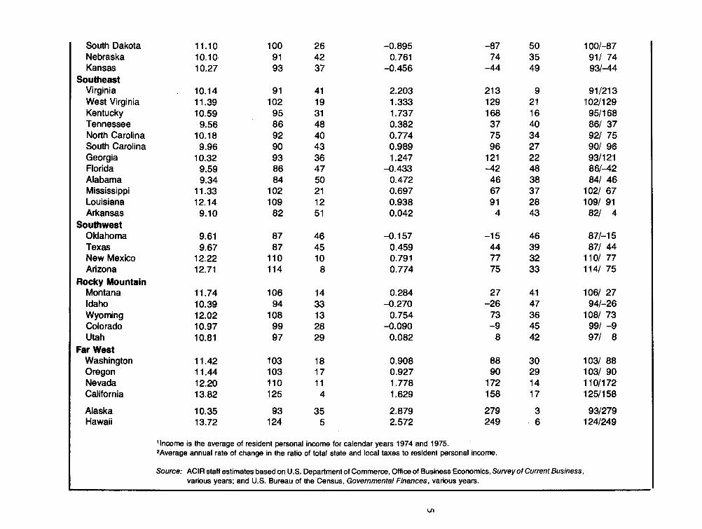
Table I develops a fiscal pressure index which includes a time span dimension. Column 1 is the ratio of own-source tax collections to resident personal income for 1975. The ratios are indexed based on the United States' median and ranked accordingly in Columns 2 and 3 . In 1975, fiscal pressure ranged from a low of 9.1 % in Arkansas to a high of 16.2% in New York.

Column 4 presents estimates of the average annual rate of change in tax effort from 1964 to 1975.4 Columns 5 and6 index these rates of change based on the U.S. median and show their relative ranking. For eight states - South Dakota, Iowa, Colorado, North Dakota, ~daho , Kansas, Oklaho- ma, and Florida - tax pressure actually fell between 1964 and 1975. Note the degree of diversity in growth among the states. The range of growth rates was from an average increase of 3.069% per year in New York to a fall of 1.031% per year in North Dakota for a differential of 4.1% per year. In index number terms, the difference was almost 400% between these two states.

Column 7 combines these two dimensions into a single measure of "fiscal blood pressure" based on each state's index numbers. The numerator or "systolic" reading indicates the state's relative position in 197 5. The denominator or "diastolic" measurement indicates the state's relative change in pressure from 1964 to 1975. Thus, the median state's fiscal pressure becomes 100 over 100.

4Average annual rate of change in the ratio of total state and local taxes to resident personal income.

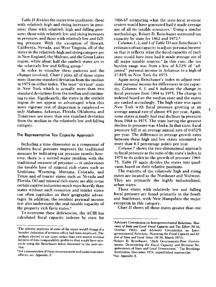
Table I 1 divides the states into quadrants: those with relatively high and rising increases in pressure; those with relatively high and falling pressure; those with relatively low and rising increases in pressure; and those with relatively low and falling pressure. With the exception of Hawaii, California, Nevada, and West Virginia, all of the states in the relatively high and rising category are in New England, the Mideast, and the Great Lakes region, while about half the sunbelt states are in the relatively low and falling group.'

In order to visualize these patterns and the changes involved, Chart I plots all of those states more than one standard deviation from the median in 1975 on either index. The most "deviant" state is New York which is actually more than two standard deviations from the median and continuing to rise. Significantly, the states in the sunbelt region do not appear so advantaged when this more rigorous test of dispersion is employed - only Alabama, Arkansas, Florida, Oklahoma, and Tennessee are more than one standard deviation from the median in the relatively low and falling category.

The Representative Tax Capacity Approach

Including a time dimension as a component of relative fiscal pressure improves the traditional measure by indicating tax pressure trends; however, there is a second major problem with the traditional measure of pressure - it understates the taxable base of mineral rich states such as Louisiana, Wyoming, Montana, Colorado, and Texas and of tourist states such as Nevada and Florida. Oil and mineral rich states are able to tax certain captive industries much more heavily than states without such resources and tourist states can often capitalize on their geographic advantages. In addition, the resident personal income test also understates the real taxable capacity of the property rich farm states6

To overcome these deficiencies, the ACIR has calculated fiscal capacity indexes by state for

'The relative positions of some of the states would change if a broader definition of revenue effort had been employed. The authors elected to use taxes rather than own-source revenue because of data comparability problems that would have aris- en in using the Reischauer index discussed in the next sec- tion.

6For apresentation of these overstatement and understatement effects, see Appendix A.

1966-67 estimating what the state-local revenue system would have generated had i t made average use of all its taxable resources.' Using a similar methodology, Robert D. Reischauer estimated tax capacity by state for 1962 and 1972.8

Columns I , 2, and 3 of Table 111 use Reischauer's estimates of tax capacity to adjust personal income so that i t reflects what the fiscal capacity of each state would have been had i t made average use of all major taxable source^.^ In this case, the tax burden range was from a low of 8.22% of "adjusted" personal income in Arkansas to a high of 17.83% in New York for 1975.

Again using Reischauer's index to adjust resident personal income for differences in tax capacity, Columns 4, 5, and 6 indicate the change in fiscal pressure from 1964 to 1975. The change is indexed based on the median state and the states are ranked accordingly. The high state was again New York with fiscal pressure growing at an average annual rate of almost 4% per year. Again,

3

some states actually had real declines in pressure from 1964 to 1975. The state having the greatest decline in pressure was Alaska. In that state, fiscal pressure fell at an average annual rate of 0.652% per year. The difference in average growth rates between these high and low states amounted to more than 4.3 percentage points per year.

Column 7 shows the two-dimensional approach to fiscal pressure as the ratio of the state's index in 1975 to its index in the growth of pressure 1964- 75. Table IV again divides the states into quadrants based on their relative positions.

The majority of the relatively high and rising states are located in the Northeast and Midwest. They are primarily the highly industralized, urban states.

Those states with relatively low and falling fiscal pressure are found primarily in the South and Southwest, with New Hampshire the major exception in this category.

Chart I 1 shows all those states greater than one

'Advisory Commission on Intergovernmental Relations, Mea- sures of State and Local Fiscal Capacity and Tax Effort (M-16, October 1962), and Advisory Commission on Inter- governmental Relations, Measuring the Fiscal Capacity and Ef- fort of State and Local Areas (M-58, March 1971). 8Robert D. Reischauer, "Rich Governments-Poor Govern- ments: Determining the Fiscal Capacity and Revenue Re- quirements of State and Local Government," The Brookings Institution, December 1974, unpublished manuscript.

9See Appendix B.

Nebraska Kansas

Southeast Virginia West Virginia Kentucky Tennessee North Carolina South Carolina Georgia Florida Alabama Mississippi Louisiana Arkansas

Southwest Oklahoma Texas New Mexico Arizona

Rocky Mountain Montana Idaho Wyoming Colorado Utah

Far West Washington Oregon Nevada California

Alaska Hawaii

lhcome is the average of resident personal income for calendar years 1974 and 1975. 2Average annual rate of change in the ratio of total state and local taxes to resident personal income.

Source: AClR staff estimates based on US. Department of Commerce, Office of Business Economics, Survey of Current Business, various years; and U.S. Bureau of the Census, Governmental Finances, various years.

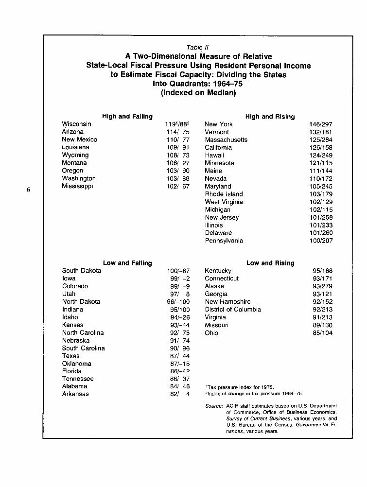
Table I1 A Two-Dimensional Measure of Relative

State-Local Fiscal Pressure Using Resident Personal Income to Estimate Fiscal Capacity: Dividing the States

Into Quadrants: 1964-75 (Indexed on Median)

High and Falling Wisconsin Arizona New Mexico Louisiana Wyoming Montana Oregon Washington Mississippi

Low and Falling South Dakota Iowa Colorado Utah North Dakota Indiana Idaho Kansas North Carolina Nebraska South Carolina Texas Oklahoma Florida Tennessee Alabama Arkansas

High and Rising New York Vermont Massachusetts California Hawaii Minnesota Maine Nevada Maryland Rhode Island West Virginia Michigan New Jersey Illinois Delaware Pennsylvania

Low and Rising Kentucky Connecticut Alaska Georgia New Hampshire District of Columbia Virginia Missouri Ohio

'Tax pressure index for 1975. 2lndex of change in tax pressure 1964-75.

Source: AClR staff estimates based on US. Department of Commerce, Office of Business Economics, Survey of Current Business, various years; and US. Bureau of the Census, Governmental Fi- nances, various years.

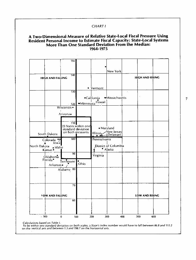
CHART l

A Two-Dimensional Measure of Relative State-Local Fiscal Pressure Using Resident Personal Income to Estimate Fiscal Capacity: State-Local Systems

More Than One Standard Deviation From the Median:

HIGH AND Rl

I I *California Massachus

blinnesI H~~~~~

Calculations based on Table I . To be within one standard deviation on both scales, a State's index number would have to fall between 86.8 and 173.2

on the vertical axis and between 1.3 and 798.7 on the horizontal axis.

State

United States Median

New England Maine New Hampshire Vermont Massachusetts Rhode Island Connecticut

Mideast New York New Jersey Pennsylvania Delaware Maryland

Table 111 A Two-Dimensional Measure of Relative State-Local Fiscal Pressure Using the Representative Tax Method to Estimate Fiscal Capacity:

~istrict of Columbia

Great Lakes Michigan Ohio Indiana Illinois Wisconsin

Plains Minnesota Iowa Missouri North Dakota

Own-Source Taxes as a Percentage of "Adjusted" Income, 1975

(1) lndex

(2)

100

114 79

119 146 124 106

171 113 112 101 121 101

118 9 5

101 11 1 126

127 99 94

102

Rank (3)

11 50

9 2 7

18

1 12 13 23

8 24

10 35 25 14 6

5 27 38 2 1

Average Annual Rate of Change in

"Adjusted" Tax Effort, 1964-75

(Percent Per Year)= (4)

lndex (5)

100

143 -27

20 38 1 281 149

537 324 244 377 347 41 9

24 1 196 98

362 29

173 -1 6 186 -3

A TWO- Dimensional Fiscal

Rank Pressure lndex (6) (7)

South Dakota Nebraska Kansas





Alaska Hawaii

'The adjustment is based on Robert Reischauer's index of fiscal capacity, op. cit. (see also Appendix B). Income is the average of resident personal income for calendar years 1974 and 1975.

2Average annual rate of change in the ratio of total state and local taxes to "adjusted" resident personal income.

Source: AClR staff estimates based on US. Department of Commerce, Office of Business Economics, Survey of Current Business, various years; and U.S. Bureau of the Census, Governmental Finances, various years.

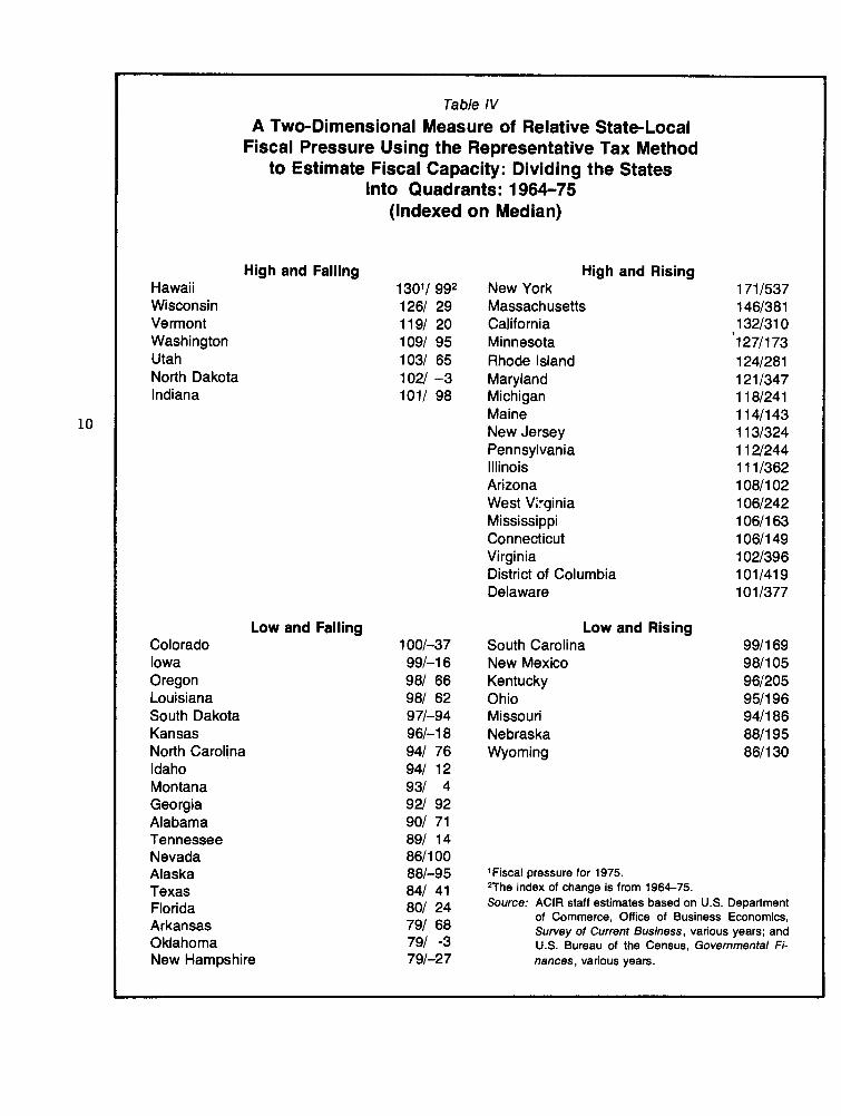
Table IV A Two-Dimensional Measure of Relative State-Local

Fiscal Pressure Using the Representative Tax Method to Estimate Fiscal Capacity: Dividing the States

Into Quadrants: 1964-75 (Indexed on Median)

High and Falling Hawaii Wisconsin Vermont Washington Utah North Dakota Indiana

Low and Falling Colorado Iowa Oregon Louisiana South Dakota Kansas North Carolina Idaho Montana Georgia Alabama Tennessee Nevada Alaska Texas Florida Arkansas Oklahoma New Hampshire

High and Rising New York Massachusetts California Minnesota Rhode Island Maryland Michigan Maine New Jersey Pennsylvania Illinois Arizona West Virginia Mississippi Connecticut Virginia District of Columbia Delaware

Low and Rising South Carolina New Mexico Kentucky Ohio Missouri Nebraska Wyoming

Fiscal pressure for 1975. 2The index of change is from 1964-75. Source: AClR staff estimates based on U.S. Department

of Commerce, Office of Business Economics, Survey of Current Business, various years; and US. Bureau of the Census, Governmental Fi- nances, various years.

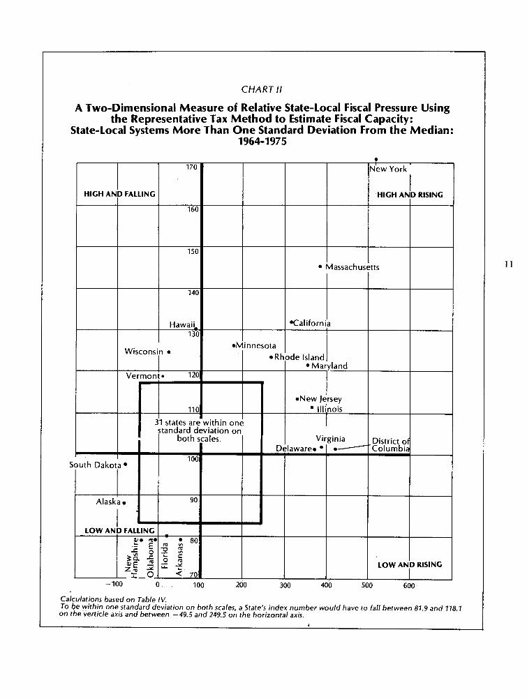
CHART 11

A Two-Dimensional Measure of Relative State-Local Fiscal Pressure Using the Representative Tax Method to Estimate Fiscal Capacity:

State-Local Systems More Than One Standard Deviation From the Median:

Calculations based on Table IV. To-be within one standard deviation on both scales, a State's index number would have to fall between 87.9 and 778.7 on the verticle axis and between -49.5 and 249.5 on the horizontal axis.

standard deviation from the median. New York is again in a class by itself, more than two standard deviations on both the index measures. Oklahoma, Florida, and Arkansas are the only states in the "growth region" that are more than one standard deviation from the median in the relatively low and falling category.

Resident Personal Income v. Representative Tax Capacity

Comparing the relative positions of the states in Table IV and Table 11 shows the difference the choice of capacity measures can make. Hawaii and Vermont move from relatively high and rising to the relatively high and falling quadrant. Connec- ticut, District of Columbia, and Virginia move from low and rising to high and rising. A number of states, including Alaska and New Hampshire,

l 2 move into the low and falling category. Finally, Nevada changes from high and rising to low and falling.

Adjusting income for what would have been available under a representative tax system makes the regional distinctions much more pronounced. There are, however, some practical problems as- sociated with this approach. The first and most important is that the data necessary to make the adjustments are not available on an annual basis. Thus, the accuracy of the adjustment process itself for any given year can be questioned. Second, the adjustment process is complicated and not easily explained or understood. In deciding which of these indexes to use, one must weight the cost of the data problems and the increased complica- tions against the improvements in accuracy.

WARNING SIGNS

A number of conclusions can be drawn from this two-dimensional measure of fiscal pressure. First, while there is a great deal of diversity in relative fiscal balance among the states, this finding ordi- narily would not be a matter of concern because differences in tastes for public goods and services are an expected and justifiable characteristic of federalism. At some point, however, growing quantitative differences have qualitative effects and diversity then takes on the character of un- wanted "disparity."

Many would argue that the growing polarization

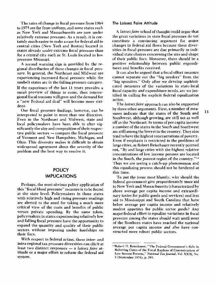
of states on this tax pressure scale has now become a "disparityH (Table 11). The data indicate that for the 1964-75 period, interstate diversity has increased- 18 states are moving toward the median, while 33 are moving away from it. For the 1953-64 period, 34 states were moving toward the median while only 17 were moving from it.I0

The Growing Diversity in State-Local Tax Pressure

Number of states moving toward median

Number of states moving away from median

A crossover appears to have occurred since 1964. Maine, Rhode Island, Maryland, Pennsyl- vania, and Illinois all moved from relatively low and rising to relatively high and rising. North Dakota, South Dakota, Colorado, Iowa, Utah, Idaho, and Florida crossed from high and falling to low and falling. Some states, such as Massa- chusetts, moved in unpredicted directions, from high and falling to high and rising. The regional patterns are in general as one would expect, with Southern and Western states moving to positions of reduced fiscal pressure while Northeast and Midwest states are moving to positions of increased pressure."

'OSummary statistics also indicate increasing diversity. For the actual burden, both the standard deviation and the coefficient of variation were less for 1964 than 1953 and greater for 1975 than 1964. For the growth in burden the coefficient of variation was much greater in 1975 than in 1964 while the standard deviation was slightly smaller. In general, the statistics indicate a movement toward equalization from 1953 to 1964 and since 1964 a movement away from equalization.

1953 1964 1975 Tax Tax Tax 1953-64 1964-75

Burden Burden Burden Growth Growth

Standard Deviation 1.45 1.28 1.46 1.06 1.02

Coefficient of Variation 0.179 0.128 0.132 0.487 0.987

"These results are based on unpublished ACIR staff compila- ations for the 1953-64 period.

The rates of change in fiscal pressure from 1964 to 1975 are far from uniform, and some states such as New York and Massachusetts are now under relatively extreme pressure. As a result, i t is certainly much easier to make a case for federal aid to central cities (New York and Boston) located in states already under extreme fiscal pressure than for a central city such as St. Louis located in low pressure Missouri.

A second warning sign is provided by the regional distribution of these changes in fiscal pressure. In general, the Northeast and Midwest are experiencing increased fiscal pressure while the sunbelt states are in the falling pressure category. If the experience of the last 11 years provides a sneak preview of things to come, then interre- gional fiscal tensions will grow and the demand for a "new Federal aid deal" will become more stri- dent.

Our fiscal pressure findings, however, can be interpreted to point in more than one direction. Even in the Northeast and Midwest, state and local policymakers have been able to alter significantly the size and composition of their respec- tive public sectors - compare the fiscal pressure of Vermont and New Hampshire, Michigan, and Ohio. This diversity makes it difficult to obtain widespread agreement about the severity of the problem and the best way to resolve it.

POLICY IMPLICATIONS

Perhaps, the most obvious policy application of this "fiscal blood pressure" measure is to be found at the state level. Policymakers in those states with relatively high and rising pressure readings are alerted to the need for taking a much more critical view of the costs and benefits of public versus private spending. By the same token, policymakers in states experiencing relatively low and falling fiscal pressure have the opportunity to expand the quantity and quality of their public sectors without imposing undue hardships on their fiscs.

With respect to federal action, these inter- and intra-regional tax pressure diversities can elicit at least two distinct responses - a laissez faire attitude or a major effort to reform the federal aid system.

The Laissez Faire Attitude

A laissez faire school of thought could argue that the great variations in state fiscal pressure do not constitute a convincing argument for major changes in federal aid flows because these diversities in fiscal pressure are due primarily to individual state choices concerning the size and shape of their public fiscs. Moreover, there should be a positive relationship between public expenditures and benefits received.

It can also be argued that a fiscal effort measure cannot separate out the "big needers" from the "big spenders." Only after we develop sophisticated measures of the variations in state-local fiscal capacity and expenditure needs, are we jus- tified in calling for explicit federal equalization action.

The laissez faire approach can also be supported by three other arguments. First, a number of measures indicate that the states of the South and 1 3

Southwest, although growing, are still not as well off as the Northeast. In terms of per capita income a number of the states in the South and Southwest are still among the lowest in the country. They also tend to have the highest concentrations of poverty. Even if emphasis is restricted to the problems of large cities, as Robert Reischauer recently pointed out, "By and large cities with the highest relative concentrations of low income persons are located in the South, the poorest region of the ~ o u n t r y . " ' ~ Thus we are seeing a catch-up phenomenon and this equalizing process should not be hiridered at this time.

To put the issue most bluntly, why should the federal government give proportionately more aid to New York and Massachusetts (characterized by above average per capita income and extraordinary tastes for public goods and services) and less aid to Mississippi and South Carolina that have below average per capita income and relatively modest appetites for public sector goods? Any major federal effort to equalize variations in fiscal pressure among the states should wait until most of the Southern states have reached the national average per capita income and also have con- structed more robust public sectors.

"Robert D. Reischauer, "The Federal Government's Role in Relieving Cities of the Fiscal Burdens of Concentrations of Low-Income Persons," Natwnal Tax journal, Vol. X X I X , No. 3 (September 1976), p. 295.

Second, there is evidence that the high spending states are beginning to place a lid on the rate of growth of expenditures. For example, Governor Lucey of Wisconsin instructed his state agencies that in preparing their 1977-79 budget proposals "new programs . . . should not be funded from new taxes but from the reallocation of existing revenue and from programs which can be reduced or eliminated." He went on to add that "increases in the number of state employees be restricted to the rate of growth of private employment in Wis- consin, if it is to grow at all."" Similar kinds of statements are being made by the governors of New York and Massachusetts.

Finally, in all of the explanations about federal spending imbalance no mention has been made of the fact that the generally higher tax bracket resi- dents of the Northeast and Midwest are able to write off a larger proportion of their heavier state

14 and local taxes against their federal income tax liability than are the relatively poorer taxpayers in the South and West. This indirect federal subsidy reduces interstate differences in real tax burdens.

The Activist Attitude

The second way to view these diversities is from the perspective of the activist. Under this view, corrective federal action is necessary now and the longer such action is delayed the more severe the problem will become. In support of this view is the fact that the disparities in economic activity appear to be increasing rather than subsiding and there is little reason to believe this trend can be quickly altered through individual state actions.

Moreover, high fiscal blood pressure readings chalked up by New York and Massachusetts are at least partially due to adverse, regional economic trends -not to an extraordinary increase in their regional appetites for public sector goods. For example, for the 1964-75 period New York State experienced only about average growth in own- source state and local tax collections but its average income growth rate was 1.6% less than the U.S. average. Texas on the other hand also had about average growth in tax collections, but its personal income growth rate was more than 1 percentage point higher than the U. S. average.

A number of those high pressure states, par-

"Governor Patrick J . Lucey, "Press Release," State Capital Building, Madison, Wisconsin, July 9, 1976, pp. 1-2.

ticularly New York and Massachusetts, are also bearing far more than their proportionate share of the national welfare burden. By aiding the federal government in carrying out this responsibility, they are in the process weakening their own fiscal position. These "generous" public welfare states become more attractive to the out-of-state poor and less attractive to their own upper income taxpayers. It should also be noted that all of the states with high and rising fiscal pressure, except Nevada and West Virginia, are also above the median in welfare burden. (See Appendix C.)

Our categorical aid system with its stimulating matchingrequirements works against slow growth state and local governments in at least three important ways. First, it places them at acompetitive disadvantage in the intergovernmental scramble for new federal aid dollars. For example, both "low pressure" Texas and Houston are now in a far better position to take advantage of any new federal matching programs than are New York State and New York City caught in the throes of fiscal apoplexy. Second, even if governments suffering from high fiscal blood pressure come up with the necessary matching funds, the price may well be a further deterioration of their relative fiscal position. Third, federal matching and expenditure maintenance requirements make it extremely difficult for a government such as New York City to take the right "cure" for high fiscal blood pressure. For example, should that government cut out a low priority federal aid program that brings in $2 from Washington for every $1 raised locally, or alternatively should it cut back on one of its own high priority programs financed primarily with local tax dollars?

As long as we had sustained economic growth throughout the nation, these three adverse effects of federal matching were not too apparent. Sharp- ly varying regional growth rates may now force major reform of our federal aid system.

What Could Be Done

If one accepts the activist point of view then there are at least three major policy options available. The first and most far reaching would be a major redesign of our federal aid system em- phasizing broad grants calculated to equalize fiscal pressure and deemphasizing narrow matching categorical aids that tend to increase fiscal pressure in all states.

A second option is the development of a welfare circuit-breaker designed to relieve a substantial part of the excessive welfare burden borne by states with high tax pressure. Such a circuit- breaker might take effect when a state is above the median in both fiscal pressure and welfare burden. In those cases, the federal government would take over some percentage, say half, of the state-local welfare burden above the median welfare burden.14 Our studies indicate that such a program could be financed by a moderate reduction in the growth rate of all other federal aid programs. (For a listing of the states and the amount of payment, see Appendix C.)

A third approach would call for the scaling down of the matching requirements of federal aid programs for those states that are characterized by both relatively slow economic growth and above average tax pressure. Such a fiscal need might be based on a number of indicators, including not only our two-dimensional estimates of fiscal pressure but also changes in population, real personal income and manufacturing employment.

Equipped with the proper expenditure safeguards,'= the latter two approaches would provide federally financed incentives to the "high pressure" states to reduce their rate of expenditure increase while, at the same time, reducing the pain of transition. Thus, in sharp contrast to typi- cal federal fiscal incentives, these proposals would dampen rather than stimulate state-local expenditures.

The activist must still face the realization that the art of measuring differences in the need for federal aid is most primitive. Our first two- dimensional index improves the state of the art by including a time dimension. However, resident personal income, a factor upon which i t is based, has been shown to be of questionable value as a proxy for measuring tax capacity in some states.

I4To make sure that a substantial amount of federal aid goes to those jurisdictions experiencing greatest fiscal stress - the major central cities in the Northeast and Midwest - Con- gress might well require the states to pass through a substantial part of this welfare reimbursement to local governments on a highly equalizing basis.

"Such expenditure safeguards might include the requirements that state-local expenditures in general and welfare expenditures in particular would not be eligible for prefer- ential federal funding if they exceeded national rates of growth.

While our second two-dimensional index improves the reliability of interstate comparisons, the dataconstraints and the complexities inherent in "adjusting" state personal income figures make its ready acceptance doubtful. Thus, as is often the case, the activist is left in the unhappy position of either recommending policy changes based on im- precise ,information or waiting until better data become available.

The real activist, however, will be willing to settle for less than perfect information, realizing that as always there are only three types of data - the non-existent, the inadequate, and the forth- coming.

SUMMARY

In this paper we have attempted to build a more sophisticated gauge of state-local fiscal stress. A "fiscal blood pressure" type of index was con- 15 structed that measures state-local tax pressure at both a given time and over time. In order to increase its reliability this two-dimensional index was then adapted to the ACIR representative tax model for estimating state-local fiscal capacity.

This more sophisticated fiscal blood pressure type of index ~roduced readings that revealed greater pressure differences between the nation's slow and fast growing regions than could be ob- tained with the traditional measure - state and local taxes as a percent of resident personal income at a given point in time.

By placing the 50 state-local systems and the District of Columbia into fiscal pressure quadrants, it also became readily apparent that regional tax pressure diversities are both extensive and growing. Significant differences in tax pressure readings among states within the same region, however, certainly complicate any attempt to pre- scribe nationwide solutions.

Finally, we set forth several explanations for the great variations in fiscal pressure readings among the states, and then showed how these explanations could be used to support two sharply differ- ing philosophies of political behavior - a laissez faire approach, or reforms that would tailor federal aid to the varying rates of economic growth and fiscal pressure among the states and localities. These reforms could include equalizing block grants, public welfare circuit-breakers, or variable federal matching requirements.

Appendix A

The Understatement or Overstatement of Tax Pressure When the Conventional Tax Effort Measure Is Compared to the

Representative Tax Yield Measure

1975 Tax Effort Difference

State Conventional Representative

Measure* Measurea

New England Maine 12.3 New Hampshire 10.3 Vermont 14.7 Massachusetts 13.9 Rhode Island 11.5 Connecticut 10.4

Mideast New York 16.2 17.8 New Jersey 11.2 11.8 Pennsylvania 11.1 11.7 Delaware 11.2 10.6 Maryland 11.7 12.7 District of Columbia 10.2 10.6

Great Lakes Michigan 11.4 Ohio 9.5 Indiana 10.6 Illinois 11.2 Wisconsin 13.2

Plains Minnesota 13.4 Iowa 11 .O Missouri 9.9 North Dakota 10.7

Percent Percent Overstated Understated

South Dakota Nebraska Kansas





Alaska Hawaii

'State and local tax collections as percent of resident personal income. %tat@ and local tax collections as percent of representative tax base.

Appendix B

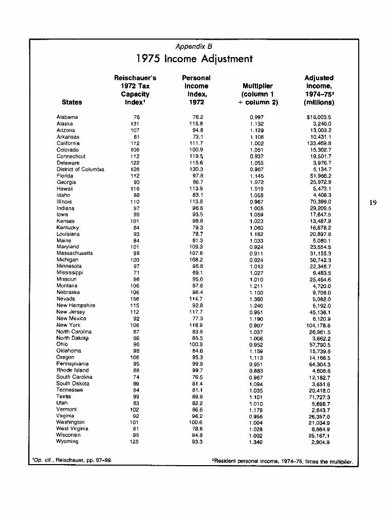
1975 Income Adjustment Appendix Table B illustrates the way in which

this adjustment works. Column I is Reischauer's index of adjusted tax capacity for 1972. It may be stated as: TCi/POPi+zTCi/&POPi where

1 1

TCi = the tax capacity for the ith state in 1972. It is the actual dollar amount which would have been collected by the ith state in 1972 had they made average use of all of their taxable resources.

POPi = the population of the ith state in 1972.

zTCi =the tax capacity of all state-local govern- 18 1 ments in the United States in 1972. It is

equal to total state-local government tax collections in 1972.

ZPOPi = the United States' population in 1972.

Column I 1 is an index of personal income in 1972. It may be written: PIi/POPi+CPIi/ZE'OPi where 1 1

PIi = resident personal income of the ith state in 1972.

ZPIi = personal income of the United States in 1972.

Column 111 is simply Column I divided by Col- umn 11. It may be written: TCi/PIi+zTCi/ZPIi.

I i

If for any given year the ratio of a state's tax capacity based on average use of all its taxable resources to its personal income is greater than the U.S. average, personal income underestimates the relative true tax capacity of that state. If the state's ratio of tax capacity to personal income is less than the U.S. average, personal income overestimates the relative tax capacity of the state. Thus Column 111 provides a multiplier which is used to correct personal income for differences in taxable resources among the states. Column IV uses this multiplier to adjust average 1975 personal income correcting for differences in tax capacity.

The final step in the process is to divide state- local own-source, tax collections in 1975 by the adjusted personal income figure. Using the adjustment process, the 1975 tax burden of New York, for example, is changed from 16.2% to 17.8% while that of Nevada is changed from 12.2% to 9%.

States

Alabama Alaska Arizona Arkansas California Colorado Connecticut Delaware District of Columbia Florida Georgia Hawaii Idaho Illinois Indiana Iowa Kansas Kentucky Louisiana Maine Maryland Massachusetts Michigan Minnesota Mississippi Missouri Montana Nebraska Nevada New Hampshire New Jersey New Mexico New York North Carolina North Dakota Ohio Oklahoma Oregon Pennsylvania Rhode Island South Carolina South Dakota Tennessee Texas Utah Vermont Virginia Washington West Virginia Wisconsin Wyoming

Op. cit., Reischauer, pp. 97-99.

Appendix B

1 975 Income Adjustment

Reischauer's 1972 Tax Capacity

Index1

Personal Income Index, 1972

76.2 115.8 94.8 73.1 111.7 100.9 119.5 115.6 130.3 97.8 86.7 113.9 83.1

1 13.8 96.6 93.5 98.8 79.3 78.7 81.3 109.3 107.6 108.2 95.8 69.1 95.0 87.6 96.4 114.7 92.8 117.7 77.3

1 1 6.9 83.9 85.5 100.8 84.6 95.3 99.9 99.7 76.5 81.4 81.1 89.9 82.2 86.6 96.2 100.6 78.8 94.8 93.3

Multiplier (column 1

+ column 2)

Adjusted Income, 1 974-7s2 (millions)

$1 6,003.5 3,240.0 13,003.2 10,431.1 133,469.8 15,302.7 19,501.7 3,976.7 5,134.7 51,966.2 25,972.9 5,473.1 4,408.3 70,399.0 29,209.5 17,647.5 13,487.9 16,878.2 20,897.8 5,080.1 23,554.5 31,155.3 50,742.3 22,346.7 9,483.5 25,464.6 4,720.0 9,708.0 5,082.0 5,192.0 45,136.1 6,120.9

104,178.8 26,961.5 3,662.2 57,790.5 15,739.6 14,166.5 64,304.3 4,606.6 12,182.7 3,651.6 20,418.0 71,727.3 5,698.7 2,643.7 26,357.0 21,034.9 8.664.9 25,167.1 2,904.9

. . 2Resident personal income, 1974-75, times the multiplier.

Appendix C

Public Welfare Circuit-Breaker Plan,

Amount of Federal Reimbursement to States for Excess Public

Welfare Payments: 1975'

States with Welfare Burden Above Median

Welfare Burden (State-Local

Welfare Expenditures

from Own Funds as Percent of State Personal Income)

State and Local Welfare

Expenditures from Own Funds

(in millions)

Excess Payments Reimbursement

(in millions) 100 Percent 50 Percent

District of Columbia Massachusetts Michigan California Rhode Island

New York Hawaii Pennsylvania Wisconsin Minnesota

Vermont New Hampshire Maine New Jersey Illinois

Ohio Oregon Iowa Kentucky Delaware

Maryland Connecticut Washington Alaska Colorado

Total

1Excess payments means public welfare expenditures above those of the median state (above 0.76% of state personal income). Source: AClR staff computations.

measuring the fiscal - unt

Documents