measuring the effects of unconventional monetary policy … · measuring the effects of...
TRANSCRIPT

NBER WORKING PAPER SERIES
MEASURING THE EFFECTS OF UNCONVENTIONAL MONETARY POLICYON ASSET PRICES
Eric T. Swanson
Working Paper 21816http://www.nber.org/papers/w21816
NATIONAL BUREAU OF ECONOMIC RESEARCH1050 Massachusetts Avenue
Cambridge, MA 02138December 2015
I thank Mike Woodford for encouraging me to write this paper, and Sofia Bauducco and participantsat the Central Bank of Chile Annual Conference for helpful discussions, comments, and suggestions. I gratefully acknowledge funding from the Central Bank of Chile for this research. The views expressedin this paper are my own and do not necessarily reflect the views of the individuals or groups listedabove. All errors and omissions are my own. The views expressed herein are those of the author anddo not necessarily reflect the views of the National Bureau of Economic Research.
NBER working papers are circulated for discussion and comment purposes. They have not been peer-reviewed or been subject to the review by the NBER Board of Directors that accompanies officialNBER publications.
© 2015 by Eric T. Swanson. All rights reserved. Short sections of text, not to exceed two paragraphs,may be quoted without explicit permission provided that full credit, including © notice, is given tothe source.

Measuring the Effects of Unconventional Monetary Policy on Asset PricesEric T. SwansonNBER Working Paper No. 21816December 2015JEL No. E44,E52,E58
ABSTRACT
I adapt the methods of Gurkaynak, Sack, and Swanson (2005) to estimate two dimensions of monetarypolicy during the 2009-2015 zero lower bound period in the U.S. I show that, after a suitable rotation,these two dimensions can be interpreted as "forward guidance" and "large-scale asset purchases" (LSAPs).I estimate the sizes of the forward guidance and LSAP components of each FOMC announcementbetween January 2009 and June 2015, and show that those estimates correspond closely to identifiablefeatures of major FOMC announcements over that period. Forward guidance has relatively small effectson the longest-maturity Treasury yields and essentially no effect on corporate bond yields, while LSAPshave large effects on those yields but essentially no effect on short-term Treasuries. Both types ofpolicies have significant effects on medium-term Treasury yields, stock prices, and exchange rates.
Eric T. SwansonDepartment of EconomicsUniversity of California at Irvine3151 Social Science PlazaIrvine, CA 92697-5100and [email protected]
1
1. Introduction
On December 16, 2008, the U.S. Federal Reserve’s Federal Open Market Committee (FOMC)
lowered the federal funds rate—its traditional monetary policy instrument—to essentially zero
in response to the most severe U.S. financial crisis since the Great Depression. Because U.S.
currency carries an interest rate of zero, it is essentially impossible for the FOMC to target a
value for the federal funds rate that is substantially less than zero. Faced with this zero lower
bound (ZLB) constraint, the FOMC subsequently began to pursue alternative, “unconventional”
monetary policies, with particular emphasis on forward guidance and large-scale asset purchases
(defined below). In this paper, I propose a new method to identify and estimate the effects of
these two main types of unconventional monetary policy.
Understanding the effects of unconventional monetary policy is an important topic for both
policymakers and researchers. Many central banks around the world have found themselves
constrained by the zero lower bound on short-term nominal interest rates. Central banks faced
with this constraint must pursue unconventional monetary policy if they wish to affect financial
markets and/or the economy. Understanding the effects of different types of unconventional
monetary policy, then, allows policymakers and researchers to better understand the efficacy,
strengths, and weaknesses of the various alternatives.
The effectiveness of unconventional monetary policy is also an important determinant of
the costs of the zero lower bound constraint. If unconventional monetary policy is relatively
ineffective, then the ZLB constraint is more costly, and policymakers should go to greater lengths
to prevent hitting the ZLB in the first place—such as by choosing a higher target rate of inflation,
as advocated by several authors (see Blanchard, Dell’Ariccia, and Mauro, 2010; The Wall Street
Journal, 2010; and Ball, 2014). On the other hand, if unconventional monetary policy is very
effective, then the ZLB constraint is much less costly and policymakers do not need to take such
drastic action to avoid hitting it in the future.
In the present paper, I focus on measuring the effects of forward guidance and large-scale
asset purchases in particular, since those were the two types of unconventional monetary policy
used most extensively by the Federal Reserve during the recent U.S. ZLB period. The term
“forward guidance” refers to communication by the FOMC about the likely future path of the
federal funds rate over the next several quarters or years. “Large-scale asset purchases” (or
LSAPs) refers to purchases by the Federal Reserve of hundreds of billions of dollars’ worth of
longer-term assets, such as long-term U.S. Treasuries and mortgage-backed securities. The goals of

2
Table 1: Major Unconventional Monetary Policy Announcements
by the Federal Reserve, 2009–2015
March 18, 2009 FOMC announces it expects to keep the federal funds rate between 0 and25 basis points (bp) for “an extended period”, and that it will purchase$750B of mortgage-backed securities, $300B of longer-term Treasuries,and $100B of agency debt (a.k.a. “QE1”)
November 3, 2010 FOMC announces it will purchase an additional $600B of longer-termTreasuries (a.k.a. “QE2”)
August 9, 2011 FOMC announces it expects to keep the federal funds rate between 0 and25 bp “at least through mid-2013”
September 21, 2011 FOMC announces it will sell $400B of short-term Treasuries and usethe proceeds to buy $400B of long-term Treasuries (a.k.a. “OperationTwist”)
January 25, 2012 FOMC announces it expects to keep the federal funds rate between 0 and25 bp “at least through late 2014”
September 13, 2012 FOMC announces it expects to keep the federal funds rate between 0 and25 bp “at least through mid-2015”, and that it will purchase $40B ofmortgage-backed securities per month for the indefinite future
December 12, 2012 FOMC announces it will purchase $45B of longer-term Treasuries permonth for the indefinite future, and that it expects to keep the federalfunds rate between 0 and 25 bp at least as long as the unemploymentremains above 6.5 percent and inflation expectations remain subdued
December 18, 2013 FOMC announces it will start to taper its purchases of longer-term Trea-suries and mortgage-backed securities to paces of $40B and $35B permonth, respectively
December 17, 2014 FOMC announces that “it can be patient in beginning to normalize thestance of monetary policy”
both policies was to lower longer-term U.S. interest rates using methods other than changes in the
current federal funds rate. Both types of unconventional monetary policy were used extensively by
the Federal Reserve, as can be seen in Table 1. Note that, in addition to the major unconventional
monetary policy announcements listed in Table 1, there was incremental news about these policies
that was released to financial markets at almost every FOMC meeting, such as updates that a
policy was ongoing, was likely to be continued, or might be adjusted.
A major challenge in identifying and estimating the effects of the FOMC’s unconventional
monetary policy announcements is determing the size and type of each announcement. For ex-
ample, many of the statements in Table 1 were at least partially anticipated by financial markets
prior to their official release. Because financial markets are forward-looking, the anticipated com-
ponent of each announcement should not have any effect on asset prices; only the unanticipated
component should be news to financial markets and have an effect. But determining the size of
the unexpected component of each announcement in Table 1 is very difficult, because there are no

3
good data on what financial markets expected the outcome of each FOMC announcement to be.1
A closely related issue is that the FOMC can sometimes surprise markets through its
inaction rather than its actions. For example, on September 18, 2013, financial markets widely
expected the FOMC to begin tapering its LSAPs, but the FOMC decided not to do so, sur-
prising markets and leading to a large effect on asset prices despite the fact that no action was
announced.2 This implies that even dates not listed in Table 1 could have produced a significant
surprise in financial markets and led to large effects on asset prices and the economy.
Determining the type—forward guidance vs. LSAP— of any given announcement can also
be very difficult. For example, many announcements in Table 1 clearly contain significant news
about both types of policies, which makes disentangling the news on those dates challenging.
Even in the case of a seemingly clear-cut announcement, both types of policies may be at work:
in particular, several authors have argued that LSAPs affect the economy by changing financial
market expectations about the future path of the federal funds rate (see, e.g., Woodford, 2012;
Bauer and Rudebusch, 2014). To the extent that this channel is operative, even a pure LSAP
announcement would have important forward guidance implications. This makes disentangling
the two types of policies even more difficult than it might at first seem.
In this paper, I address these problems by adapting the methods of Gurkaynak, Sack,
and Swanson (2005, henceforth GSS) to the zero lower bound period in the U.S., from 2009
to 2015. The problem GSS faced was similar to the problem I face here, in that GSS were
interested in separately identifying the effects of two dimensions of monetary policy: changes in
the current federal funds rate vs. changes in the FOMC’s forward guidance. In the zero lower
bound environment I consider here, there are also two dimensions of monetary policy, but now
those two dimensions are different: changes in forward guidance and LSAPs. (Changes in the
current federal funds rate are not a significant component of monetary policy during this period
because of the zero lower bound constraint on the funds rate.)
Following GSS, I look at how financial markets responded in a 30-minute window brack-
eting each FOMC announcement between 2009 and 2015, and compute the first two principal
components of those asset price responses. The idea is that forward guidance and LSAPs were
1 In contrast, for conventional monetary policy—changes in the federal funds rate—federal funds futures andother short-term financial market instruments provide very good measures of market expectations leading up toeach announcement. See Kuttner (2001), Gurkaynak, Sack, and Swanson (2005, 2007), and others.
2For example, The Wall Street Journal reported that “No Taper Shocks Wall Street,” and “‘Bernanke had afree pass to begin that tapering process and chose not to follow [through]. . . The Fed had the market preciselywhere it needed to be. The delay today has the effect of raising the benchmark to tapering. . . ” (The Wall StreetJournal, 2013b,c).

4
by far the two most important components of FOMC announcements for financial markets, and
thus their effects should be well captured by the first two principal components of the asset price
responses. I then search over all possible rotations of these two principal components to find the
specification in which one of the two factors has the clearest interpretation as a “forward guid-
ance” factor, using the estimated effect of forward guidance from the pre-ZLB period (computed
exactly as in GSS) as the benchmark for what the effects of forward guidance should look like.
The remaining, orthogonal factor can then be interpreted as the second main dimension of mon-
etary policy during this period. I interpret this second factor as measuring the FOMC’s LSAP
announcements and present evidence that supports this interpretation. For example, I plot both
of these factors—forward guidance and LSAPs—over time and show that they fit identifiable
features of major FOMC announcements over the period quite well. In this way, I separately
identify the size of the forward guidance and LSAP component of every FOMC announcement
between January 2009 and June 2015.
Once the FOMC’s forward guidance and LSAP announcements are identified, it’s then
straightforward to estimate the effects of each type of announcement on the high-frequency re-
sponse of different types of asset prices around those announcements.
The remainder of the paper proceeds as follows. In Section 2, I review the analytical
methods of GSS, show how to adapt them to the recent ZLB period, and describe the data. In
Section 3, I perform the principal component analysis and rotate the factors as described above.
I plot the estimated factors over time and discuss their relationship to identifiable features of
major announcements by the FOMC over the ZLB period, showing that my estimates of forward
guidance and LSAP announcements seem to be well identified and informative. In Section 4, I
estimate the effects of these announcements on Treasury yields, stock prices, exchange rates, and
corporate bond yields and spreads. In Section 5, I discuss the implications of my findings for
monetary policy going forward.
2. Methods and Data
My methods in the present paper consist of two main steps. First, I extend the analysis of
Gurkaynak, Sack, and Swanson (2005) through December 16, 2008, which was the last time the
FOMC announced a change in the federal funds rate target. (After December 16, 2008, the
funds rate was essentially at a level of zero, and the FOMC was unable or unwilling to lower the

5
federal funds rate any further.) This allows me to identify and estimate the effects of changes
in the federal funds rate and changes in forward guidance in “normal times”, before the ZLB
began to bind.3 Second, I adapt the methods of GSS to the ZLB period from January 2009
through June 2015, during which the FOMC never changed the current federal funds rate target
but made multiple unconventional monetary policy announcements involving forward guidance
and large-scale asset purchases, as noted in Table 1. I thus use the GSS methods, applied to the
ZLB sample, to identify and estimate the effects of forward guidance and LSAPs during this later
period.
I extend the GSS dataset through June 2015 using data obtained from staff at the Federal
Reserve Board. The combined dataset includes the date of each FOMC announcement from July
1991 through June 2015, and the change in a number of asset prices in a 30-minute window
bracketing each announcement.4 The asset prices include federal funds futures rates (contracts
with expiration at the end of the current month and each of the next five months), eurodollar
futures rates (contracts with expiration near the end of the current quarter and each of the
next seven quarters), Treasury bond yields (for the 3-month, 6-month and 2-, 5-, 10-, and 30-
year maturities), the stock market (as measured by the S&P 500), and the U.S. dollar-yen and
dollar-euro exchange rates.
To replicate the GSS analysis over the pre-ZLB period, I focus on the responses of the
first and third federal funds futures contracts, the second, third, and fourth Eurodollar futures
contracts, and the 2-, 5-, and 10-year Treasury yields to each FOMC announcement from July
1991 through December 2008. The two federal funds futures contracts can be scaled so as to
provide good estimates of the market expectation of what the federal funds rate will be after
the current and next FOMC meetings (see GSS, 2005, for details). The second through fourth
Eurodollar futures contracts provide information about the market expectation of the path of the
federal funds rate over the horizon from about 4 months to 1 year ahead.5 The 2-, 5-, and 10-year
3My results are very similar if I end the sample in December 2004, as GSS did, or in December 2007.
4The window begins 10 minutes before the FOMC announcement and ends 20 minutes after the FOMC an-nouncement. The dataset also includes the dates and times of FOMC announcements and some intraday asset priceresponses going back to January 1990, but the data for Treasury yield responses begins in July 1991, and those dataare an important part of my analysis. Also, as is standard in the literature, I exclude the FOMC announcementon September 17, 2001, which took place after financial markets had been closed for several days following theSeptember 11 terrorist attacks. I also include the Federal Reserve Board’s announcement on November 25, 2008,that it would begin purchasing mortgage-backed securities and GSE debt (the beginning of “QE1”)—although thisannouncement was not made by the FOMC itself, all subsequent asset purchase announcements were made by theFOMC, so I include it with those others. However, including or excluding this announcement does not noticeablyaffect any of my results.
5The reason for focusing on some rather than all of the possible futures contract rates in the dataset is to avoid

6
Treasury yields provide information about interest rate expectations and risk premia over longer
horizons, about 1 to 10 years.
These asset price responses to FOMC announcements can be written as a matrix X, with
rows of X corresponding to FOMC announcements and columns of X corresponding to different
futures rates and Treasury yields. Since there are 159 FOMC announcements from July 1991
through December 2008, and I focus on 8 asset price responses, the matrix X has dimensions
159× 8.
As in GSS, I use principal component analysis to estimate the two factors that make the
most important contribution to the variation in X. The idea is that the asset price responses in
X are well described by a factor model,
X = FΛ + ε, (1)
where F is a 159×2 matrix containing two factors, Λ is a 2×8 matrix of loadings of the asset price
responses on the two factors, and ε is a 159× 8 matrix of white noise residuals. Letting F denote
the first two principal components of X, the two columns of F represent the two components of
the FOMC’s announcements that have had the greatest impact on the assets in X over the period
from July 1991 to December 2008.
Although the first two principal components of X explain a maximal fraction of the variation
in X, they are only a statistical decomposition and typically do not have a structural interpreta-
tion. In order to associate one column of F with changes in the federal funds rate and the other
column with changes in forward guidance—which is a structural interpretation—it’s necessary to
transform the factor matrix F so that it fits this interpretation.
Keeping this goal in mind, note that if F and Λ characterize the data X in equation (1),
and U is any 2× 2 orthogonal matrix, then the matrix ˜F ≡ FU and loadings ˜Λ ≡ U ′Λ represent
an alternative factor model that fits the data X exactly as well as F and U , in the sense that it
overlapping contracts as much as possible, since they are highly correlated for technical rather than policy-relatedreasons. When I conduct the principal components analysis of the data below, futures contracts that are highlycorrelated will tend to show up as a common factor, which would not be interesting if the correlation was generatedby overlapping contracts rather than the way monetary policy is conducted. For example, FOMC announcementsare generally spaced 6 to 8 weeks apart, so there is essentially no gain to including the second federal fundsfutures contract in addition to the first—the second contract is very highly correlated with the first fed fundsfutures contract, once the latter contract has been scaled to represent the outcome of the current FOMC meeting.Similarly, including the first Eurodollar futures contract would provide essentially no additional information beyondthe first and third fed funds futures contracts. I follow GSS and switch from federal funds futures to Eurodollarfutures contracts at a horizon of about 2 quarters because Eurodollar futures were much more liquid over thissample than longer-maturity fed funds futures, and are thus likely to provide a better measure of financial marketexpectations at those longer horizons (see Gurkaynak, Sack, and Swanson, 2007).

7
produces exactly the same residuals ε in equation (1).6 Ideally, we would like the two columns
of F to correspond to changes in the federal funds rate and changes in the FOMC’s forward
guidance, as mentioned above. Although the first two principal components of X do not in
general have this interpretation, we can choose a rotation matrix U such that the rotated factors
˜F do have such an interpretation. In particular, we can choose U such that, if f1 and f2 are
the two columns of ˜F , then f2 has no effect on the current federal funds rate.7 This implies
that all of the variation in the current federal funds rate (up to the white noise residuals ε) in
response to FOMC announcements is due to changes in the first factor, f1. The factor f1 can
thus be interpreted as the surprise component of the FOMC’s change in the federal funds rate
target. The second factor, f2, then corresponds to all of the other information in the FOMC’s
announcements, above and beyond the surprise change in the funds rate, that changed financial
market expectations about the future path of the funds rate. Thus, f2 can be thought of as
“forward guidance” by the FOMC.8 As GSS show, the second factor f2, identified in this way,
corresponds closely to important changes in the FOMC’s statements about the outlook for the
future path of monetary policy, supporting the interpretation of f2 as the change in the FOMC’s
forward guidance.
I next adapt this methodology to the zero lower bound period in the U.S., from January 2009
to June 2015. As in GSS and discussed above, I create a data matrix X with rows corresponding
to FOMC announcements between January 2009 and June 2015, and columns corresponding to
the responses of different futures rates and bond yields in a narrow, 30-minute window bracketing
each announcement. However, I exclude the first and third federal funds futures contracts and the
second Eurodollar futures contract from this analysis, because those contracts have such short
maturities that they essentially do not respond to news during the ZLB period.9 The matrix
X that I construct for the ZLB sample thus has dimensions 52 × 5, corresponding to the 52
FOMC announcements over this period, and 5 different asset price responses: the third and
6The scale of F and Λ are also indeterminate: if k is any scalar, then kF and Λ/k also fit the data X exactlyas well as F and Λ. Traditionally, the scale of F is normalized so that each column has unit variance.
7 In other words, λ21 = 0, where λij denotes the (i, j)th element of ˜Λ, so the current-month federal funds futurescontract is not affected by changes in the second factor.
8GSS called f1 the “target factor” and f2 the “path factor”, because it relates to the future path of the federalfunds rate, but the latter is now typically referred to as “forward guidance”.
9The first and third federal funds futures contracts correspond to federal funds rate expectations over the next1 and 3 months, respectively, and the second Eurodollar futures contract corresponds to funds rate expectationsfrom about three to six months ahead. As shown by Swanson and Williams (2014), interest rates at these shortmaturities essentially stopped responding systematically to news from 2009 to 2012 (the end of their sample), andthis remains true through about mid-2015.

8
fourth Eurodollar futures contracts and the 2-, 5-, and 10-year Treasury yields.
As in GSS and discussed above, I extract the first two principal components from the
matrix X. These are the two features of FOMC announcements between 2009 and mid-2015
that moved the five yields listed above the most. As before, these two principal components do
not have a structural interpretation in general. Let F zlb denote the 52 × 2 matrix of principal
components, let U be a 2 × 2 orthogonal matrix, let ˜F zlb ≡ F zlbU , and let fzlb1 and fzlb
2 denote
the first and second columns of ˜F zlb. I search over all possible rotation matrices U to find the one
where the first rotated factor fzlb1 is as close as possible (in terms of its asset price effects) to the
“forward guidance factor” f2 estimated previously (over the 1991–2008 sample).10 The identifying
assumption is thus that the effect of forward guidance on medium- and longer-term interest rates
during the ZLB period is about the same as it was during the pre-ZLB period from 1991–2008.
The remaining factor, fzlb2 , then corresponds to the component of FOMC announcements, above
and beyond changes in forward guidance, that have the biggest effect on medium- and longer-
term interest rates. It is natural to interpret this second factor as corresponding to the FOMC’s
large-scale asset purchases.
The crucial assumption underlying this identification is that forward guidance has essen-
tially the same effects on medium- and longer-term interest rates before and after the ZLB. This
assumption is subject to debate, but it provides a natural starting point for my analysis and
in fact seems to work very well, as I show below. Thus, for every FOMC announcement from
January 2009 through June 2015, I can separately identify the forward guidance component and
the LSAP component of that announcement. Once I’ve separately identified the two components,
it’s straightforward to estimate the effects of each component on asset prices using ordinary least
squares regressions.
3. The FOMC’s Forward Guidance and LSAP Announcements
I now report the results of these methods applied to the pre-ZLB and ZLB periods.
3.1 Federal Funds Rate and Forward Guidance Factors before the ZLB
Table 2 reports the rotated loading matrices ˜Λ from the estimation procedure described above.
The first two rows report results for the pre-ZLB period, July 1991 to December 2008. Each factor,
10 In other words, I choose the rotation matrix U that matches the factor loadings λzlb11 , λzlb
12 , λzlb13 , λzlb
14 , and λzlb15
to λ24, λ25, λ26, λ27, and λ28 as closely as possible, in the sense of minimum Euclidean distance.

9
Table 2: Estimated Effects of Conventional and Unconventional Monetary
Policy Announcements on Interest Rates before and after Dec. 2008
MP1 MP2 ED2 ED3 ED4 2y Tr. 5y Tr. 10y Tr.
July 1991–Dec. 2008:
(1) change in federal funds rate 8.55 6.23 5.88 5.59 4.81 3.79 1.91 0.68(2) change in forward guidance 0.00 1.18 4.23 5.42 6.12 5.08 5.20 4.02
Jan. 2009–June 2015:
(3) change in forward guidance — — — 3.18 4.15 3.33 4.24 2.35(4) change in LSAPs — — — −0.73 −0.99 −1.27 −4.90 −7.46
memo:
(5) row 3, rescaled — — — 4.68 6.11 4.89 6.24 3.45
Coefficients in the table correspond to elements of the loading matrix Λ from equation (1), in basis pointsper standard deviation change in the monetary policy instrument (except for row 5, which is rescaled).MP1 and MP2 denote scaled changes in the first and third federal funds futures contracts, respectively;ED2, ED3, and ED4 denote changes in the second through fourth Eurodollar futures contracts; and 2y,5y, and 10y Tr. denote changes in 2-, 5-, and 10-year Treasury yields. See text for details.
f1 and f2, is normalized to have a unit standard deviation over this sample, so the coefficients
in the table are in units of basis points (bp) per standard deviation change in the monetary
policy instrument. A one-standard-deviation increase in the federal funds rate over this period
is estimated to cause the current federal funds rate to rise by about 8.6bp, the expected federal
funds rate at the next FOMC meeting to rise about 6.2bp, the second through fourth Eurodollar
futures rates to rise by 5.9, 5.6, and 4.8bp, respectively, and the 2-, 5-, and 10-year Treasury
yields to increase by 3.8, 1.9, and 0.7bp, respectively. The effects of a surprise change in the
federal funds rate are thus largest at the short end of the yield curve and die off monotonically
as the maturity of the interest rate increases.
The effects of forward guidance, in the second row, are quite different. By construction, a
shock to the forward guidance factor has no effect on the current federal funds rate. At longer
maturities, however, the forward guidance factor’s effects increase, peaking at a maturity of about
one year, and then dying off slightly for longer maturities. Thus, changes in forward guidance
have a roughly hump-shaped effect on the yield curve. For longer-term yields, such as the 5- and
10-year yields, changes in forward guidance are a far more important source of variation than are
changes in the federal funds rate, as originally emphasized by GSS.
3.2 Forward Guidance and LSAP Factors during the ZLB Period
The third and fourth rows of Table 2 report the rotated loadings ˜Λ for the ZLB period from

10
January 2009 through June 2015. The third row reports the effects of a one-standard-deviation
change in forward guidance on the third and fourth Eurodollar futures contract and the 2-, 5-,
and 10-year Treasury yields, respectively. By construction, these coefficients match those in the
second row as closely as possible, up to a constant scale factor, so the effect of forward guidance
is hump-shaped with a peak at intermediate maturities of about 1 year. (For reference, the fifth
row of Table 2 rescales the coefficients in row 3 so that their correspondence to the second row
can be seen more easily.)
The fourth row reports the effects of a one-standard-deviation increase in the FOMC’s asset
purchases. I normalize the sign of this factor so that an increase in purchases causes interest
rates to fall. The effect on yields is relatively small at short and medium horizons but increases
steadily with maturity—exactly the opposite of changes in the current federal funds rate. At a
horizon of one year, the effect of LSAPs is only about 1bp, but for the 10-year Treasury yield,
the effect is more than seven times larger, about 7.5bp.
3.3 Correspondence of Factors to Notable FOMC Announcements
In Figure 1, I plot the time series of estimated values of the forward guidance and LSAP factors
for each FOMC announcement from January 2009 to June 2015. The dashed blue line depicts the
forward guidance factor, and the solid orange line the LSAP factor. To make the interpretation of
the LSAP factor more intuitive, I scale it by −1 in the figure, so that an increase in LSAPs appears
as a negative value; this sign convention implies that positive values in the figure correspond to
monetary policy tightenings and negative values to monetary policy easings. The figure also
contains brief annotations that help to explain some of the larger observations in the figure.
The largest and most striking observation in Figure 1 is the negative 5.5-standard-deviation
LSAP announcement on March 18, 2009, near the beginning of the ZLB sample. This observation
corresponds to the announcement of the FOMC’s first LSAP program, often referred to as “QE1”
in the press.11 The key elements of this program are listed in Table 1, and the announcement seems
to have been a major surprise to financial markets, given the huge estimated size of the factor on
that date. Note that my identification procedure for forward guidance vs. LSAP announcements
described above attributes the effects of this announcement to the LSAP factor. Given that this
11The “QE1” program began on November 25, 2008, when the Federal Reserve Board announced it would pur-chase $600 billion of mortgage-backed securities and $100 billion of debt issued by the mortgage-related government-sponsored enterprises. The term “QE1” typically refers to both this earlier program and the huge expansion ofthat program announced on March 18, 2009.

11
Figure1:EstimatedForward
Guidanceand
LSAP
Factors,2009–2015
6543210123standarddeviations
Estim
ated
forw
ard
guid
ance
fact
orEs
timat
edLS
APfa
ctor
"QE1
"
"Ope
ratio
nTw
ist"
FOM
Cde
cide
sno
tto
tape
r
"tap
erta
ntru
m"
"mid
2013
"
FOM
C"p
atie
nt"
inra
isin
gra
tes
FOM
Csi
gnal
scau
tion
inra
isin
gra
tes
FOM
Cex
tend
sLS
APen
dda
tefr
om20
09Q
4to
2010
Q1
Plotofestimatedforw
ard
guidance
(dashed
blueline)
andLSAP
(solidorangeline)
factors,fzlb
1andfzlb
2,ov
ertime.
Notable
FOMC
announcemen
tsare
labeled
inthefigure
forreference.TheLSAP
factoris
multiplied
by−1
inthefigure
sothatpositivevalues
inthe
figure
correspondto
interest
rate
increases.
See
textfordetails.
12
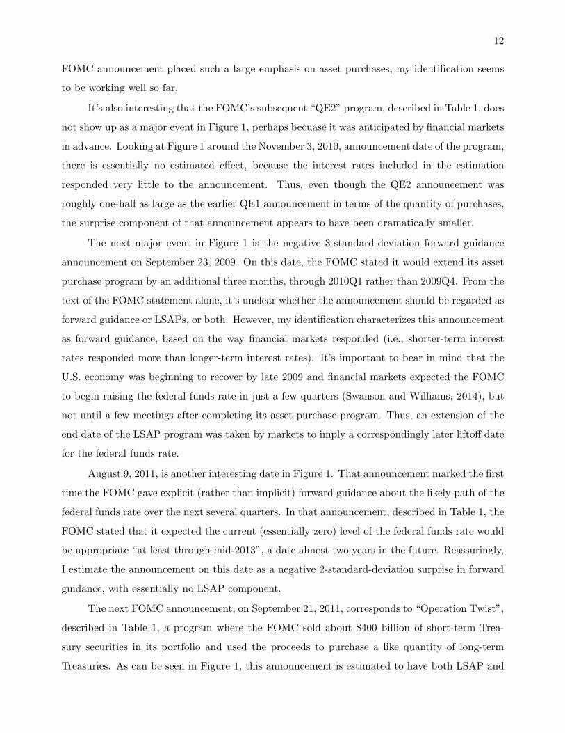
FOMC announcement placed such a large emphasis on asset purchases, my identification seems
to be working well so far.
It’s also interesting that the FOMC’s subsequent “QE2” program, described in Table 1, does
not show up as a major event in Figure 1, perhaps becuase it was anticipated by financial markets
in advance. Looking at Figure 1 around the November 3, 2010, announcement date of the program,
there is essentially no estimated effect, because the interest rates included in the estimation
responded very little to the announcement. Thus, even though the QE2 announcement was
roughly one-half as large as the earlier QE1 announcement in terms of the quantity of purchases,
the surprise component of that announcement appears to have been dramatically smaller.
The next major event in Figure 1 is the negative 3-standard-deviation forward guidance
announcement on September 23, 2009. On this date, the FOMC stated it would extend its asset
purchase program by an additional three months, through 2010Q1 rather than 2009Q4. From the
text of the FOMC statement alone, it’s unclear whether the announcement should be regarded as
forward guidance or LSAPs, or both. However, my identification characterizes this announcement
as forward guidance, based on the way financial markets responded (i.e., shorter-term interest
rates responded more than longer-term interest rates). It’s important to bear in mind that the
U.S. economy was beginning to recover by late 2009 and financial markets expected the FOMC
to begin raising the federal funds rate in just a few quarters (Swanson and Williams, 2014), but
not until a few meetings after completing its asset purchase program. Thus, an extension of the
end date of the LSAP program was taken by markets to imply a correspondingly later liftoff date
for the federal funds rate.
August 9, 2011, is another interesting date in Figure 1. That announcement marked the first
time the FOMC gave explicit (rather than implicit) forward guidance about the likely path of the
federal funds rate over the next several quarters. In that announcement, described in Table 1, the
FOMC stated that it expected the current (essentially zero) level of the federal funds rate would
be appropriate “at least through mid-2013”, a date almost two years in the future. Reassuringly,
I estimate the announcement on this date as a negative 2-standard-deviation surprise in forward
guidance, with essentially no LSAP component.
The next FOMC announcement, on September 21, 2011, corresponds to “Operation Twist”,
described in Table 1, a program where the FOMC sold about $400 billion of short-term Trea-
sury securities in its portfolio and used the proceeds to purchase a like quantity of long-term
Treasuries. As can be seen in Figure 1, this announcement is estimated to have both LSAP and
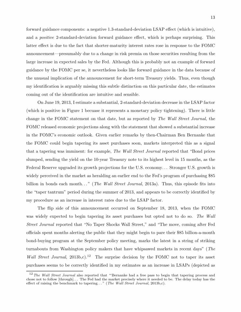
13
forward guidance components: a negative 1.3-standard-deviation LSAP effect (which is intuitive),
and a positive 2-standard-deviation forward guidance effect, which is perhaps surprising. This
latter effect is due to the fact that shorter-maturity interest rates rose in response to the FOMC
announcement—presumably due to a change in risk premia on those securities resulting from the
large increase in expected sales by the Fed. Although this is probably not an example of forward
guidance by the FOMC per se, it nevertheless looks like forward guidance in the data because of
the unusual implication of the announcement for short-term Treasury yields. Thus, even though
my identification is arguably missing this subtle distinction on this particular date, the estimates
coming out of the identification are intuitive and sensible.
On June 19, 2013, I estimate a substantial, 2-standard-deviation decrease in the LSAP factor
(which is positive in Figure 1 becuase it represents a monetary policy tightening). There is little
change in the FOMC statement on that date, but as reported by The Wall Street Journal, the
FOMC released economic projections along with the statement that showed a substantial increase
in the FOMC’s economic outlook. Given earlier remarks by then-Chairman Ben Bernanke that
the FOMC could begin tapering its asset purchases soon, markets interpreted this as a signal
that a tapering was imminent: for example, The Wall Street Journal reported that “Bond prices
slumped, sending the yield on the 10-year Treasury note to its highest level in 15 months, as the
Federal Reserve upgraded its growth projections for the U.S. economy. . . Stronger U.S. growth is
widely perceived in the market as heralding an earlier end to the Fed’s program of purchasing $85
billion in bonds each month. . . ” (The Wall Street Journal, 2013a). Thus, this episode fits into
the “taper tantrum” period during the summer of 2013, and appears to be correctly identified by
my procedure as an increase in interest rates due to the LSAP factor.
The flip side of this announcement occurred on September 18, 2013, when the FOMC
was widely expected to begin tapering its asset purchases but opted not to do so. The Wall
Street Journal reported that “No Taper Shocks Wall Street,” and “The move, coming after Fed
officials spent months alerting the public that they might begin to pare their $85 billion-a-month
bond-buying program at the September policy meeting, marks the latest in a string of striking
turnabouts from Washington policy makers that have whipsawed markets in recent days” (The
Wall Street Journal, 2013b,c).12 The surprise decision by the FOMC not to taper its asset
purchases seems to be correctly identified in my estimates as an increase in LSAPs (depicted as
12The Wall Street Journal also reported that “‘Bernanke had a free pass to begin that tapering process andchose not to follow [through]. . . The Fed had the market precisely where it needed to be. The delay today has theeffect of raising the benchmark to tapering. . . ” (The Wall Street Journal, 2013b,c).

14
a negative value in Figure 1 since it is a monetary policy easing).
Near the end of my sample, on December 17, 2014, markets expected the FOMC to remove
its statement that it would keep the federal funds rate at essentially zero “for a considerable time”.
Not only did the FOMC leave that phrase intact, it announced that “the Committee judges it
can be patient in beginning to normalize the stance of monetary policy,” which was substantially
more dovish than financial markets had expected.13 This announcement thus appears to be
correctly identified by my estimation as a large, negative 2.5-standard deviation decrease in
forward guidance by the FOMC.
Finally, on March 18, 2015, the FOMC revised its projections for U.S. output, inflation, and
the federal funds rate substantially downward, significantly below what markets had expected.
The revised forecast was read by financial markets “as a sign that the central bank would take
its time in raising borrowing costs for the economy. . . ” (The Wall Street Journal, 2015a,b).
Again, my estimation appears to correctly identify this announcement as a substantial, negative
3-standard-deviation change in forward guidance.
3.4 Scale of Forward Guidance and LSAP Factors
The forward guidance and LSAP factors estimated above and plotted in Figure 1 are normalized
to have a unit standard deviation over the sample. Similarly, the loadings in Table 2 are for
these normalized factors and thus represent a basis points per standard deviation effect. For
practical policy applications, however, it’s more useful to convert these factors to a scale that is
less abstract and more tangible.
For forward guidance, it’s natural to think of the factor in terms of a 25bp effect on the
Eurodollar future rate one year ahead, ED4. Note that a forward guidance announcement of this
size would be very large by historical standards, equal to about a 6-standard-deviation surprise
during the ZLB period, or a 4-standard-deviation surprise in the pre-ZLB period.14 To estimate
the effects of a forward guidance announcement of this magnitude, we can multiply the coefficients
in the third row of Table 2 by a factor of about 6, which implies that the effects on the 5- and
13For example, “U.S. stocks surged. . . after the Federal Reserve issued an especially dovish policy statement atthe conclusion of the FOMC meetings,” (The Wall Street Journal, 2014).
14 Interestingly, I estimate that the FOMC’s forward guidance announcements were larger on average before theZLB than during the ZLB, as can be seen in Table 2. One explanation for why this may be is that, once theFOMC issued its “mid-2013” forward guidance, there were essentially no updates or news about that guidance formany meetings. Similarly, after the FOMC revised the guidance to “late 2014”, there were again no updates ornews about that guidance for many more meetings, and so on.

15
10-year Treasury yields would be about 25.5 and 14.2bp, respectively. The interpretation is that,
if the FOMC gave forward guidance for the federal funds rate that was about 25bp lower one year
ahead than financial markets expected, then the 5- and 10-year Treasury yields would decline by
about 25.5 and 14.2bp on average.
For LSAPs, we would like the units to be in billions of dollars of purchases, which is a more
difficult transformation than a simple renormalization of the coefficients in Table 2. Nevertheless,
a number of estimates in the literature suggest that a $600 billion LSAP operation in the U.S.,
distributed across medium- and longer-term Treasury securities, leads to a roughly 15bp decline
in the 10-year Treasury yield (see, e.g., Swanson, 2011, and Table 1 of Williams, 2013). Using
this estimate as a benchmark implies that the coefficients in the fourth row of Table 2 correspond
to a roughly $300 billion surprise LSAP announcement. Thus, it seems reasonable to interpret
the coefficients in that row of Table 2 as corresponding to a $300 billion change in purchases. The
interpretation is thus that, if the FOMC announced a new LSAP program that was about $300
billion larger than markets expected, the effects would be about as large those provided in the
fourth row of Table 2.
4. The Effects of Forward Guidance and LSAPs on Asset Prices
Once we’ve identified the forward guidance and LSAP components of the FOMC’s announce-
ments from 2009 through 2015, it’s relatively straightforward to estimate the effects of those
announcements on asset prices, using ordinary least squares regressions, as follows.
4.1 Treasury Yields
Table 3 reports the responses of 6-month and 2-, 5-, 10-, and 30-year Treasury yields to the
forward guidance and LSAP components of the FOMC’s announcements. As in previous tables
and figures, the coefficients here are in units of basis points per standard deviation surprise in the
announcement. Each column of the table reports estimates from an OLS regressions of the form
Δyt = α+ β ˜F zlbt + εt, (2)
where t indexes FOMC announcements between January 2009 and June 2015, y denotes the
corresponding Treasury yield, Δ denotes the change in a 30-minute window bracketing each

16
Table 3: Estimated Effects of Forward Guidance and LSAPs on
U.S. Treasury Yields, 2009–2015
6-month 2-year 5-year 10-year 30-year
change in forward guidance 0.53∗∗∗ 3.33∗∗∗ 4.24∗∗∗ 2.35∗∗∗ 0.30
(std. err.) (.092) (.217) (.252) (.263) (.737)
[t-stat.] [5.75] [15.33] [16.82] [8.91] [0.40]
change in LSAPs −0.08 −1.27∗∗∗ −4.90∗∗∗ −7.46∗∗∗ −5.78∗∗∗
(std. err.) (.080) (.077) (.556) (.453) (.493)
[t-stat.] [−0.99] [−16.48] [−8.82] [−16.47] [−11.71]
Regression R2 .47 .93 .94 .97 .77
# Observations 52 52 52 52 52
Coefficients β from regressions Δyt = α + β˜F zlbt + εt, where t indexes FOMC announcements between
Jan. 2009 and June 2015, y denotes a given Treasury yield, ˜F denotes the forward guidance and LSAPfactors estimated previously, and Δ is the intraday change in a 30-minute window bracketing each FOMCannouncement. Coefficients are in units of basis points per standard deviation change in the monetarypolicy instrument. Huber-White heteroskedasticity-consistent standard errors in parentheses; t-statisticsin square brackets; ∗∗∗ denotes statistical significance at the 1% level. See text for details.
FOMC announcement, ˜F zlb denotes the forward guidance and LSAP factors as estimated above,
ε is a regression residual, and α and β are parameters.
The point estimates for the 2-, 5-, and 10-year Treasury yields in Table 3 are the same
as those in Table 2. However, Table 3 also reports Huber-White heteroskedasticity-consistent
standard errors and t-statistics for each coefficient, from which we can see that the responses of
these yields to both forward guidance and LSAPs are extraordinarily statistically significant, with
t-statistics ranging from 8.8 to almost 17. The regression R2 values are also quite high, over 93
percent, so these two factors explain a very large share of the variation in those yields around
FOMC announcements.
Table 3 also reports results for the 6-month and 30-year Treasury yields, which were not
included in the estimation of the factors themselves.15 LSAPs do not have a statistically significant
effect on the 6-month Treasury yield, and the effect of forward guidance on this yield is statistically
significant but small, amounting to only about 0.5bp per standard deviation surprise, less than
one-sixth the size of the 2-year Treasury yield response. This is likely due to the fact that the
6-month Treasury yield was very close to zero and largely unresponsive to news over much of this
period (Swanson and Williams, 2014). To the extent that the 6-month Treasury yield was pinned
15Results for the 3-month Treasury yield are not reported, since the 3-month Treasury yield generally did notrespond to news over this period, as shown by see Swanson and Williams (2014).

17
Table 4: Estimated Effects of Forward Guidance and LSAPs on
Stock Prices and Exchange Rates, 2009–2015
S&P500 $/euro $/yen
change in forward guidance −0.19∗∗∗ −0.25∗∗∗ −0.20∗∗∗
(std. err.) (.070) (.037) (.040)
[t-stat.] [−2.68] [−6.66] [−5.04]
change in LSAPs 0.20∗∗∗ 0.33∗∗∗ 0.37∗∗∗
(std. err.) (.053) (.049) (.050)
[t-stat.] [3.66] [6.65] [7.32]
Regression R2 .27 .67 .80
# Observations 52 52 52
Coefficients β from regressions Δ log xt = α+β˜F zlbt +εt, where t indexes FOMC announcements between
Jan. 2009 and June 2015, x is the asset price, ˜F denotes the forward guidance and LSAP factors estimatedpreviously, and Δ is the intraday change in a 30-minute window bracketing each FOMC announcement.Coefficients are in units of percentage points per standard deviation change in the monetary policyinstrument. Huber-White heteroskedasticity-consistent standard errors in parentheses; t-statistics insquare brackets; ∗∗∗ denotes statistical significance at the 1% level. See text for details.
to zero for a significant part of the sample, we wouldn’t expect to see much of a response to any
type of announcement.
The effect of forward guidance on the 30-year Treasury yield is also quantitatively small
and, in this case, statistically insignificant. In contrast to the 6-month Treasury, the 30-year
Treasury yield was not pinned to zero for any length of time during this period, so the small
coefficient reflects the fact that forward guidance apparently had little effect on the longest-
maturity Treasuries during the ZLB period. The effect of LSAPs on the 30-year Treasury yield,
however, are large and extraordinarily statistically significant, with a t-statistic of almost 12.
Interestingly, the effects of LSAPs on the 30-year yield were not quite as large as their effects on
the 10-year yield, presumably because the FOMC’s LSAP operations were typically concentrated
around maturities closer to 10 years.
4.2 Stock Prices and Exchange Rates
Table 4 reports analogous regression results for the S&P 500 stock index and dollar-euro and
dollar-yen exchange rates. The form of the regressions is the same as in equation (2), except the
dependent variable in each regression is now 100 times the log change in the asset price in each
column.
As can be seen in Table 4, both forward guidance and LSAPs have statistically significant

18
effects on stock prices and exchange rates. For stocks, a one-standard-deviation increase in forward
guidance caused prices to fall by about 0.2 percent, while a one-standard-deviation increase in
LSAPs caused stock prices to rise by a similar amount. Both of these coefficients are highly
statistically significant, with t-statistics of about 2.7 and 3.7, respectively, and both effects are in
the direction one would expect from a standard dividend-discount model, given the interest rate
responses reported in the previous table; that is, an increase in interest rates reduces the present
value of a stock’s dividends (and may reduce the size of the dividends themselves, if the economy
contracts), which will tend to cause stock prices to fall. Finally, it’s interesting that the R2 for
this regression is much lower than those for Treasury yields, due to the high and idiosyncratic
volatility of stock prices around FOMC announcements.
The effects of forward guidance and LSAPs on the dollar are more precisely estimated.
Both the dollar-euro and dollar-yen exchange rates are expressed as the dollar price per unit of
foreign currency. In response to a one-standard-deviation increase in forward guidance, the dollar
appreciated by about 0.2 to 0.25 percent, and the effect is highly statistically significant, with t-
statistics of about 6.7 for the euro and 5 for the yen. A one-standard-deviation increase in LSAPs
causes the dollar to depreciate about 0.35 percent, and the effect is again highly statistically
significant with t-statistics of 6.6 and 7.3. Again, the effects have the signs one would expect from
uncovered interest parity, given the response of interest rates reported in Table 3. That is, an
increase in U.S. interest rates makes U.S. dollar investments more attractive relative to foreign
investments, and tends to drive the value of the dollar up.
4.3 Corporate Bond Yields and Spreads
Table 5 reports results for corporate bond yields and spreads. Corporate bonds are less frequently
traded than U.S. Treasuries, stocks, and foreign exchange, so only daily frequency corporate bond
yield data are available. Thus, the regressions in Table 5 use the one-day change in corporate
bond yields or spreads around each FOMC announcement as the dependent variable. To measure
corporate yields, I consider both the Aaa and Baa indexes of long-term seasoned corporate bond
yields from Moody’s.
As can be seen in the first row of the table, I estimate that changes in the FOMC’s forward
guidance had essentially no effect on corporate bond yields during the ZLB period. The point
estimates for both Aaa and Baa yields are small (less than one-half of one basis point per standard
deviation change in forward guidance) and statistically insignificant. Because 10-year Treasury

19
Table 5: Estimated Effects of Forward Guidance and LSAPs on
Corporate Bond Yields and Spreads, 2009–2015
Corporate Yields Spreads
Aaa Baa Aaa−10-yr. Baa−10-yr.
change in forward guidance 0.28 −0.33 −1.23∗∗ −1.85∗∗
(std. err.) (.580) (.755) (.558) (.743)
[t-stat.] [0.49] [−0.44] [−2.21] [−2.49]
change in LSAPs −4.65∗∗∗ −5.17∗∗∗ 4.25∗∗∗ 3.74∗∗∗
(std. err.) (.373) (.577) (.546) (.911)
[t-stat.] [−12.48] [−8.96] [7.79] [4.11]
Regression R2 .44 .49 .56 .55
# Observations 52 52 52 52
Coefficients β from regressions Δyt = α + β˜F zlbt + εt, where t indexes FOMC announcements between
Jan. 2009 and June 2015, y denotes the corporate bond yield or spread, ˜F denotes the forward guidanceand LSAP factors estimated previously, and Δ is the change in a one-day window bracketing each FOMCannouncement. Coefficients are in units of basis points per standard deviation change in the monetarypolicy instrument. Huber-White heteroskedasticity-consistent standard errors in parentheses; t-statisticsin square brackets; ∗∗ and ∗∗∗ denote statistical significance at the 5% and 1% levels, respectively. Seetext for details.
yields rise modestly in response to a change in forward guidance, the effect on the corporate-
Treasury yield spread is thus modestly negative, falling about 1 to 2bp in response to an increase
in guidance, and this effect is moderately statistically significant, with t-statistics of 2.2 and 2.5.
The effect of LSAPs on corporate bond yields was much larger and more significant. A
one-standard-deviation increase in LSAPs caused the Aaa and Baa yields both to fall about 5bp,
and the effect was extraordinarily statistically significant. However, the effect of LSAPs on the
10-year Treasury yield was larger than the effect on corporate bond yields, so the spread between
corporate bonds and Treasuries actually increased in response to the LSAP program.16 This
result echoes findings by earlier authors, such as Krishnamurthy and Vissing-Jorgensen (2012) and
Swanson (2011), that the Fed’s LSAP programs—which tend to be concentrated in U.S. Treasury
securities—push down Treasury yields more than they do private-sector yields. Nevertheless, the
effect on corporate bond yields that I estimate here is a bit bigger than those authors found in
their studies. For example, Swanson (2011) estimated corporate bond yields fall by about 4–5bp
16The 10-year yield response in Table 2 is estimated to be about −7.5bp, while the effect implied in Table 5 isa bit larger, about −8.9bp. There are two reasons for this difference: first, the responses in Table 2 are 30-minuteresponses, while those in Table 5 are one-day responses. Second, Table 2 uses the on-the-run coupon-bearing10-year Treasury bond, while in Table 5 I use the 10-year zero-coupon yield estimate by Gurkaynak, Sack, andWright (2007). The latter yield has a longer duration than the coupon-bearing 10-year security, which should bea better match to the long-term corporate bonds in the Moody’s indexes.

20
in response to a $600 billion Treasury LSAP, while the estimates in Table 5 are closer to 9–10bp
for the same size operation (assuming this is a roughly two-standard-deviation announcement, as
discussed earlier). One reason for the larger estimates here may be because the FOMC’s recent
LSAP programs often included a substantial quantity of mortgage-backed securities (MBS) as
well as Treasuries. Those MBS are likely to be closer substitutes for corporate bonds than are
Treasuries, so we should expect purchases of MBS to have a relatively larger effect on corporate
bond yields than purchases of Treasuries alone. The earlier estimates in Krishnamurthy and
Vissing-Jorgensen (2012) and Swanson (2011) were for the case of a Treasury-only LSAP, and
thus could be expected to have smaller effects on private yields than the MBS-and-Treasury
LSAPs conducted by the FOMC between 2009 and 2015.
5. Conclusions
In this paper, I show how to identify and estimate the forward guidance and large-scale asset
purchase component of every FOMC announcement between 2009 and 2015, the U.S. zero lower
bound period. Building on earlier work by Gurkaynak, Sack, and Swanson (2005), I estimate a
time series for each type of unconventional monetary policy announcement, and show that these
series correspond to identifiable characteristics of important FOMC statements during this period.
I use these identified forward guidance and LSAP announcements to estimate the effects of
each type of policy on Treasury yields, stock prices, exchange rates, and corporate bond yields
and spreads. I find that forward guidance affected Treasury yields at all but the very longest
maturities, with a peak effect at a maturity of about one to five years. In contrast, I find that
the effects of LSAPs increased with maturity, with LSAPs having their peak effect on the longest
maturities, 10 and 30 years. LSAPs had essentially no effect on the shortest-maturity Treasuries.
I estimate that forward guidance had no effect on corporate bond yields during the ZLB
period. In contrast, LSAPs had substantial and highly significant effects on those yields. Never-
theless, the effects of LSAPs on corporate debt was smaller than their effects on Treasuries, so
corporate bond spreads actually increased after an increase in the FOMC’s asset purchases. This
finding is consistent with others in the literature, and probably reflects the fact that the Fed’s
LSAP programs focused largely on purchases of Treasury securities.
Stock prices responded about equally to changes in forward guidance and LSAPs over the
zero lower bound period. This is perhaps surprising, given that forward guidance seems to have
been relatively unimportant for other long-duration assets, such as the 30-year Treasury and
21
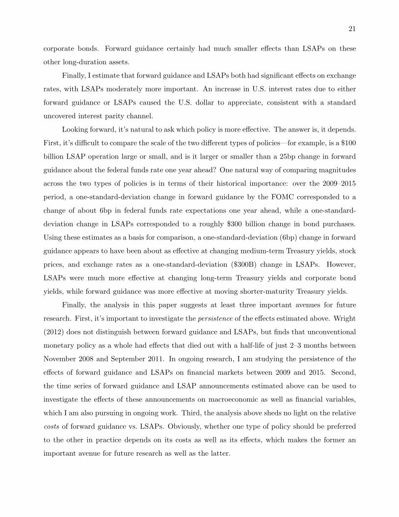
corporate bonds. Forward guidance certainly had much smaller effects than LSAPs on these
other long-duration assets.
Finally, I estimate that forward guidance and LSAPs both had significant effects on exchange
rates, with LSAPs moderately more important. An increase in U.S. interest rates due to either
forward guidance or LSAPs caused the U.S. dollar to appreciate, consistent with a standard
uncovered interest parity channel.
Looking forward, it’s natural to ask which policy is more effective. The answer is, it depends.
First, it’s difficult to compare the scale of the two different types of policies—for example, is a $100
billion LSAP operation large or small, and is it larger or smaller than a 25bp change in forward
guidance about the federal funds rate one year ahead? One natural way of comparing magnitudes
across the two types of policies is in terms of their historical importance: over the 2009–2015
period, a one-standard-deviation change in forward guidance by the FOMC corresponded to a
change of about 6bp in federal funds rate expectations one year ahead, while a one-standard-
deviation change in LSAPs corresponded to a roughly $300 billion change in bond purchases.
Using these estimates as a basis for comparison, a one-standard-deviation (6bp) change in forward
guidance appears to have been about as effective at changing medium-term Treasury yields, stock
prices, and exchange rates as a one-standard-deviation ($300B) change in LSAPs. However,
LSAPs were much more effective at changing long-term Treasury yields and corporate bond
yields, while forward guidance was more effective at moving shorter-maturity Treasury yields.
Finally, the analysis in this paper suggests at least three important avenues for future
research. First, it’s important to investigate the persistence of the effects estimated above. Wright
(2012) does not distinguish between forward guidance and LSAPs, but finds that unconventional
monetary policy as a whole had effects that died out with a half-life of just 2–3 months between
November 2008 and September 2011. In ongoing research, I am studying the persistence of the
effects of forward guidance and LSAPs on financial markets between 2009 and 2015. Second,
the time series of forward guidance and LSAP announcements estimated above can be used to
investigate the effects of these announcements on macroeconomic as well as financial variables,
which I am also pursuing in ongoing work. Third, the analysis above sheds no light on the relative
costs of forward guidance vs. LSAPs. Obviously, whether one type of policy should be preferred
to the other in practice depends on its costs as well as its effects, which makes the former an
important avenue for future research as well as the latter.
22
References
Ball, Laurence (2014). “The Case for a Long-Run Inflation Target of Four Percent,” IMF Working
Paper 14/92.
Bauer, Michael, and Glenn Rudebusch (2014). “The Signaling Channel for Federal Reserve Bond
Purchases,” International Journal of Central Banking 10, 233–289.
Blanchard, Olivier, Giovanni Dell’Ariccia, and Paolo Mauro (2010). “Rethinking Macroeco-
nomic Policy,” IMF Staff Position Note 10/03.
Gurkaynak, Refet, Brian Sack, and Eric Swanson (2005). “Do Actions Speak Louder than Words?
The Response of Asset Prices to Monetary Policy Actions and Statements,” International Journal
of Central Banking 1, 55–93.
Gurkaynak, Refet, Brian Sack, and Eric Swanson (2007). “Market-Based Measures of Monetary
Policy Expectations,” Journal of Business and Economic Statistics 25, 201–212.
Gurkaynak, Refet, Brian Sack, and Jonathan Wright (2007). “The U.S. Treasury Yield Curve:
1961 to the Present,” Journal of Monetary Economics 54, 2291–2304.
Krishnamurthy, Arvind, and Annette Vissing-Jorgensen (2012). “The Aggregate Demand for
Treasury Debt,” Journal of Political Economy 120, 233–267.
Kuttner, Kenneth (2001). “Monetary Policy Surprises and Interest Rates: Evidence from the Fed
Funds Futures Market,” Journal of Monetary Economics 47, 523–544.
Piazzesi, Monika, and Eric Swanson (2008). “Futures Prices as Risk-Adjusted Forecasts of Monetary
Policy,” Journal of Monetary Economics 55, 677–691.
Swanson, Eric, and John Williams (2014). “Measuring the Effect of the Zero Lower Bound on
Medium- and Longer-Term Interest Rates,” American Economic Review 104, 3154–3185.
Swanson, Eric (2011). “Let’s Twist Again: A High-Frequency Event-Study Analysis of Operation Twist
and Its Implications for QE2,” Brookings Papers on Economic Activity, Spring 2011, 151–188.
The Wall Street Journal (2010). “Q&A: IMF’s Blanchard Thinks the Unthinkable,” by Davis, Bob,
February 11, 2010, Real Time Economics.
The Wall Street Journal (2013a). “Bond Markets Sell Off,” by Burne, Katy, and Mike Chernev, June
19, 2013, Credit Markets.
The Wall Street Journal (2013b). “No Taper Shocks Wall Street: Fed ‘Running Scared’,” by Rusolillo,
Steven, September 18, 2013, Money Beat.
The Wall Street Journal (2013c). “Fed Stays the Course on Easy Money,” by Hilsenrath, Jon, and
Victoria McGrane, September 19, 2013, Economy.
The Wall Street Journal (2014). “U.S. Stocks Surge after Fed Gets Dovish on Policy,” by Vigna, Paul,
December 17, 2014, Money Beat.
The Wall Street Journal (2015a). “U.S. Government Bonds Rally after Fed Statement,” by Zeng, Min,
March 18, 2015, Credit Markets.
The Wall Street Journal (2015b). “U.S. Stocks Surge as Fed Seen Taking Time on Rates,” by WSJ Staff,
March 18, 2015, Money Beat.
Williams, John (2013). “Lessons from the Financial Crisis for Unconventional Monetary Policy,” panel
discussion at the NBER Conference on Lessons from the Financial Crisis for Monetary Policy,
October 18, 2013, available at http://www.frbsf.org/our-district/press/presidents-speeches/williams-
speeches/2013/october/research-unconventional-monetary-policy-financial-crisis.
Woodford, Michael (2012). “Methods of Policy Accommodation at the Interest-Rate Lower Bound,”
in The Changing Policy Landscape: Federal Reserve Bank of Kansas City Symposium Proceedings

23
from Jackson Hole, Wyoming (Kansas City: Federal Reserve Bank of Kansas City) 185–288, available
at http://www.kansascityfed.org/publications/research.
Wright, Jonathan (2012). “What Does Monetary Policy Do to Long-Term Interest Rates at the Zero
Lower Bound?” Economic Journal 122, F447–F466.