FEDERAL RESERVE BANK OF SAN FRANCISCO

WORKING PAPER SERIES

Measuring the Effect of the Zero Lower Bound On Medium- and Longer-Term Interest Rates

Eric T. Swanson Federal Reserve Bank of San Francisco

and

John C. Williams

Federal Reserve Bank of San Francisco

January 2013

The views in this paper are solely the responsibility of the authors and should not be interpreted as reflecting the views of the Federal Reserve Bank of San Francisco or the Board of Governors of the Federal Reserve System.

Working Paper 2012-02 http://www.frbsf.org/publications/economics/papers/2012/wp12-02bk.pdf

Measuring the Effect of the Zero Lower Bound

on Medium- and Longer-Term Interest Rates

Eric T. Swanson∗

and

John C. Williams∗

Federal Reserve Bank of San Francisco

January 2013

Abstract

The federal funds rate has been at the zero lower bound for over four years, since December 2008.According to many macroeconomic models, this should have greatly reduced the effectiveness ofmonetary policy and increased the efficacy of fiscal policy. However, standard macroeconomictheory also implies that private-sector decisions depend on the entire path of expected future short-term interest rates, not just the current level of the overnight rate. Thus, interest rates with ayear or more to maturity are arguably more relevant for the economy, and it is unclear to whatextent those yields have been constrained. In this paper, we measure the effects of the zero lowerbound on interest rates of any maturity by estimating the time-varying high-frequency sensitivityof those interest rates to macroeconomic announcements relative to a benchmark period in whichthe zero bound was not a concern. We find that yields on Treasury securities with a year or moreto maturity were surprisingly responsive to news throughout 2008–10, suggesting that monetaryand fiscal policy were likely to have been about as effective as usual during this period. Onlybeginning in late 2011 does the sensitivity of these yields to news fall closer to zero. We offer twoexplanations for our findings: First, until late 2011, market participants expected the funds rate tolift off from zero within about four quarters, minimizing the effects of the zero bound on medium-and longer-term yields. Second, the Fed’s unconventional policy actions seem to have helped offsetthe effects of the zero bound on medium- and longer-term rates.

Keywords: monetary policy, zero lower bound, forward guidance, fiscal policy, fiscal multiplier

JEL Classification: E43, E52, E62

∗We thank James Hamilton, Kei Kawakami, Yvan Lengwiler, Benoit Mojon, John Taylor, Min Wei, Jonathan Wright,and seminar participants at the Federal Reserve Bank of San Francisco, NBER Monetary Economics Meeting, FederalReserve Board, Federal Reserve Bank of St. Louis Conference, Society for Economic Dynamics Meetings, Haas Schoolof Business, Swiss National Bank Conference, NBER EFG Meeting, UC Irvine, Brown University, Boston University-FRB Boston Conference, Reserve Bank of Australia Conference, and AEAMeetings for helpful discussions, comments,and suggestions. We thank Maura Lynch and Kuni Natsuki for excellent research assistance. The opinions expressedin this paper are those of the authors and do not necessarily reflect the views of the people listed above, the FederalReserve Bank of San Francisco, the Board of Governors of the Federal Reserve System, or any other individualswithin the Federal Reserve System.

Swanson: Federal Reserve Bank of San Francisco, eric.swanson@sf.frb.org, http://www.ericswanson.org.

Williams: Federal Reserve Bank of San Francisco, 101 Market Street, San Francisco, CA 94105, Tel.: (415) 974-2121,John.C.Williams@sf.frb.org.

1 Introduction

The federal funds rate—the Federal Reserve’s traditional monetary policy instrument—has been

at a lower bound of essentially zero for over four years, since December 2008. However, standard

textbook macroeconomic models (e.g., Clarida, Galı, and Gertler 1999, Woodford 2003) imply that

the economy is affected by the entire path of expected future short-term interest rates, not just

the current level of the overnight rate. Thus, interest rates with a year or more to maturity are

arguably more relevant for the economy, and it is not clear whether the zero lower bound has

substantially affected the behavior of these longer-term yields. Theoretically, if a central bank

has the ability to commit to future values of the policy rate, it can work around the zero bound

constraint by promising monetary accommodation in the future once the zero bound ceases to bind

(Reifschneider and Williams 2000, Eggertsson and Woodford 2003). Empirically, Gurkaynak, Sack,

and Swanson (2005b) found that the Federal Reserve’s monetary policy announcements affect asset

prices primarily through their effects on financial market expectations of future monetary policy,

rather than changes in the current federal funds rate target. Thus, there are both theoretical and

empirical reasons to believe that monetary policy can remain effective even when the overnight

interest rate is at zero. Indeed, 1- and 2-year yields remained substantially above zero throughout

much of 2008–10 (Figure 1), suggesting that monetary policy still had room to affect the economy

despite the constraint on the current level of the federal funds rate. On several occasions, in fact, the

Federal Reserve’s Federal Open Market Committee (FOMC) generated a decline in medium- and

longer-term Treasury yields of as much as 20 basis points by managing monetary policy expectations

or purchasing assets.1

The extent to which the zero lower bound affects interest rates of different maturities also

has important implications for fiscal policy. Numerous authors have emphasized that the macroe-

conomic effects of fiscal policy are much larger when the zero lower bound is binding, because in

that case interest rates do not rise in response to higher output, and private investment is not

1For example, on August 9, 2011, the FOMC stated, “The Committee currently anticipates that economic con-ditions. . . are likely to warrant exceptionally low levels for the federal funds rate at least through mid-2013.” Inresponse to this announcement, the 2-year Treasury yield fell 8 basis points (bp), while the 5- and 10-year Treasuryyields each fell 20 bp. In normal times, it would take a surprise change in the federal funds rate of about 100 bp togenerate a fall of 8 to 20 bp in intermediate-maturity yields (Gurkaynak et al. 2005b).

1

0

1

2

3

4

5

0

1

2

3

4

5

Federal Funds Rate1 Year Treasury2 Year Treasury5 Year Treasury10 Year Treasury

Figure 1. Federal funds rate target and 1-, 2-, 5-, and 10-year zero-coupon Treasury yieldsfrom January 2007 through December 2012. Data are from the Federal Reserve Board and theGurkaynak, Sack, and Wright (2007) online dataset.

“crowded out” (e.g., Christiano, Eichenbaum, and Rebelo 2011, Woodford 2011).2 However, stan-

dard macroeconomic theory implies that private-sector spending depends on the path of expected

future short-term interest rates, as mentioned above. Thus, whether the overnight rate is con-

strained by the zero lower bound today is less relevant for the size of the fiscal multiplier than

whether somewhat longer-maturity yields are constrained. Indeed, Christiano et al. (2011), Wood-

ford (2011), and others emphasize that the extent to which private spending is crowded out by

fiscal stimulus depends on the length of time that the one-period interest rate is constrained by the

zero bound.3 Put differently, those authors find that the fiscal multiplier depends on the extent to

which intermediate-maturity yields are constrained.

In this paper, we propose a novel method of measuring the extent to which interest rates of any

maturity—and hence monetary policy, more broadly defined—are affected by the zero lower bound.

2See also Eggertsson (2009), Erceg and Linde (2010), Eggertsson and Krugman (2012), and DeLong and Summers(2012).

3As discussed by those authors, the expected path of government purchases is also important. For example,the fiscal multiplier is larger the greater the fraction of government purchases that is expected to occur while theone-period interest rate is at zero. See Section 5.4, below, for additional discussion of the fiscal multiplier.

2

In particular, we estimate the time-varying sensitivity of yields to macroeconomic announcements

using high-frequency data and compare that sensitivity to a benchmark period in which the zero

bound was not a concern (taken to be 1990–2000). In periods in which a given yield is about as

sensitive to news as in the benchmark sample, we say that the yield is unconstrained. If there are

periods when the yield responds very little or not at all to news, we say that the yield is largely

or completely constrained in those periods. Intermediate cases are measured by the degree of the

yield’s sensitivity to news relative to the benchmark period, and the severity and statistical sig-

nificance of the constraint can be assessed using standard econometric techniques. This represents

the first empirical study of the effects of the zero lower bound on the behavior of intermediate- and

longer-maturity yields, and thus to what extent the zero bound has hindered the effectiveness of

monetary policy and amplified the effectiveness of fiscal policy.

We emphasize that the level of a yield alone is not a useful measure of whether that yield is

constrained by the zero lower bound, for at least three reasons. First, there is no way to quantify

the severity of the zero bound constraint or its statistical significance using the level of the yield

alone. For example, if the one-year Treasury yield is 50 basis points (bp), there is no clear way to

determine whether that yield is severely constrained, mildly constrained, or even unconstrained.

By contrast, the method we propose in this paper provides an econometrically precise answer to

this question.

Second, the lower bound on nominal interest rates may be above zero for institutional reasons,

and this “effective” lower bound may vary across countries or over time.4 For example, the Federal

Reserve has held the target federal funds rate at a floor of 0 to 25 bp from December 2008 through

at least the end of 2012, but the Bank of England has maintained a floor of 50 bp for its policy rate

over the same period while conducting unconventional monetary policy on a similar scale to the

Federal Reserve. Evidently, the effective floor on nominal rates in the U.K. is about 50 bp rather

than zero. As a result, a 50 or even 100 bp gilt yield in the U.K. might be substantially constrained

by the effective U.K. lower bound of 50 bp, while a similar 50–100 bp yield in the U.S. might be

only mildly constrained or unconstrained.5 The approach in this paper relies on the sensitivity

4See Bernanke and Reinhart (2004) for a discussion of the institutional barriers to lowering the policy rate all theway to zero.

5As another example, in 2003, the Federal Reserve lowered the funds rate to 1 percent, at which point it beganto use forward guidance, such as the phrase “policy accommodation can be maintained for a considerable period,” to

3

of interest rates to news rather than the level of rates, and thus can accommodate effective lower

bounds that may be greater than zero or change over time.

Third, the sensitivity of interest rates to news is more relevant than the level of yields for the

fiscal multiplier. As emphasized by Christiano et al. (2011), Woodford (2011), and others, what is

crucial for the fiscal multiplier is whether or not interest rates respond to a government spending

shock; the level of yields by itself is largely irrelevant. Although the zero lower bound motivates

the analysis in those studies, their results are all derived in a “constant interest rate” environment

in which nominal yields can be regarded as fixed at any absolute level.

To preview our results, we find that Treasury yields with one or two years to maturity were

surprisingly responsive to news throughout 2008–10, despite the federal funds rate being essentially

zero over this period. Contrary to conventional wisdom, this suggests that the efficacy of monetary

and fiscal policy were likely close to normal in 2008–10. Only beginning in late 2011 do we see the

sensitivity of the two-year Treasury yield to news become significantly less than normal. We also

show that Treasury yields with five or ten years to maturity were essentially unconstrained by the

zero bound throughout our sample, while Treasury yields with six months or less to maturity have

been severely constrained by the zero bound since the spring of 2009. Importantly, our method

provides a quantitative measure of the degree to which the zero bound affects each yield, as well as

a statistical test for the periods during which it was affected.

We provide two explanations for our findings. First, up until August 2011, market participants

consistently expected the zero bound to constrain policy for four quarters or less, minimizing the

zero bound’s effects on medium- and longer-term yields. Second, the Federal Reserve’s large-scale

purchases of long-term bonds and management of monetary policy expectations may have helped

to offset the effects of the zero bound on medium- and longer-term interest rates.

The remainder of the paper proceeds as follows. Section 2 lays out a simple New Keynesian

model that illustrates three important points used in our empirical analysis. Section 3 describes our

empirical framework. Our main results are reported in Section 4. Section 5 considers the broader

implications of our results and various extensions and robustness checks. Section 6 concludes.

try to lower longer-term interest rates without cutting the funds rate any further (see, e.g., Bernanke and Reinhart2004; the quotation is from the FOMC statement dated August 12, 2003). Thus, one can make a good case that theeffective lower bound on the funds rate in 2003–04 was 100 bp rather than zero.

4

2 An Illustrative Model

In this section, we use a simple macroeconomic model to illustrate the effects of the zero lower

bound on the responsiveness of yields to economic news. In particular, we use the model to

illustrate three important points that we will employ in our empirical analysis, below. First, when

short-term interest rates are constrained by the zero lower bound, yields of all maturities respond

less to economic announcements than if the zero bound were not present; moreover, the reduction

in the responsiveness of yields to news is greatest at short maturities and is smaller for longer-term

yields. Second, the effects of the zero bound on the sensitivity of yields to news is essentially

symmetric—that is, the responsiveness of yields to both positive and negative announcements falls

by about the same amount when the zero bound is strongly binding on short-term rates. Third,

the zero bound dampens the sensitivity of yields to news by similar amounts for different types of

shocks, so long as the persistence of those shocks are not too different. Readers who are willing to

take these three points for granted can skip ahead to the next section.

We conduct the analysis in this section using a standard, simple, three-equation New Keynesian

model (cf. Clarida, Galı, and Gertler (1999) and Woodford (2003), among others) that describes

the evolution over time t of the output gap, yt, inflation rate, πt, and one-period risk-free nominal

interest rate, it. The purpose of this exercise is to illustrate qualitatively how the zero lower bound

affects the sensitivity of bond yields to news, so the model is deliberately simplistic and not intended

to capture the quantitative effects we estimate below.6

The model’s output gap equation is derived from the household’s consumption Euler equation,

and relates the output gap this period to the expected output gap next period and the difference

between the current ex ante real interest rate, it − Etπt+1, and natural rate of interest, r∗t :

yt = −α(it − Etπt+1 − r∗t ) + Etyt+1. (1)

Solving this equation forward, assuming limk→∞Etyt+k = 0, we have:

yt = −αEt

∞∑

j=0

{it+j − πt+j+1 − r∗t+j}. (2)

6One could use alternative models for this section as well, such as Hamilton and Wu’s (2012) model of the zerolower bound. There are advantages and disadvantages to each type of model; we choose the standard New Keynesianframework here since it is so widely known and used.

5

This equation makes clear that the current level of the output gap depends on the entire expected

future path of short-term interest rates, inflation, and the natural rate of interest. As emphasized

by Woodford (2003) and Erceg et al. (2000), among others, the quantity Et∑∞

j=0 it+j can be

interpreted as a nominal long-term interest rate in the model.

We model shocks to the output gap as shocks to the natural interest rate, r∗t . We assume that

the natural interest rate follows a stationary AR(1) process,

r∗t = (1− ρ)r∗ + ρr∗t−1 + et, (3)

where ρ ∈ (−1, 1) and r∗ denotes the unconditional mean of the natural rate.

The equation for inflation is derived from profit maximization by monopolistically competitive

firms with Calvo price contracts, and is given by:

πt = γyt + βEtπt+1 + μt, (4)

where μt can be thought of as a markup shock, assumed to follow a stationary AR(1) process:

μt = δμt−1 + vt, (5)

where δ ∈ (−1, 1).

The one-period interest rate in the model is set according to a Taylor (1993) Rule, subject to

the constraint that it must be nonnegative:

it = max { 0, πt + r∗t + 0.5(πt − π) + 0.5yt}, (6)

where π denotes the central bank’s inflation target, taken to be 2 percent. Note that monetary

policy is assumed to respond to the current level of the natural interest rate. This implies that,

absent the zero lower bound, monetary policy perfectly offsets the effects of shocks to the natural

interest rate on the output gap and inflation. Of course, the presence of the zero lower bound

implies that, in certain circumstances, monetary policy will be unable to offset such shocks.

Consistent with the log-linearized structure of the economy implicit in equations (1)–(5), we

assume that long-term bond yields in the model are determined by the expectations hypothesis.

Thus, the M -period yield to maturity on a zero-coupon nominal bond, iMt , is given by:

iMt = Et

M−1∑

j=0

it+j + φM , (7)

6

where φM denotes an exogenous term premium that may vary with maturity M but is constant

over time.

We solve for the impulse response functions of the model under two scenarios: First, a scenario

in which the initial value of r∗t is substantially greater than zero, so that the zero lower bound is

not a binding constraint on the setting of the short-term interest rate; and second, a scenario in

which the initial value of r∗t is −4, which is sufficient for the zero bound to constrain the short-

term nominal rate it for several periods.7 In the latter case, we solve the model using a nonlinear

perfect foresight algorithm, as in Reifschneider and Williams (2000), which solves for the impulse

response functions of the model to an output or inflation shock under the assumption that the

private sector assumes that realized values of all future innovations will be zero. In each scenario,

impulse responses are computed as the difference between the path of the economy after the shock

and the baseline path of the economy absent the shock.

We set the model parameters α = 1.59 and γ = 0.096, based on Woodford (2003), and choose

illustrative values for the shock persistences of ρ = 0.85 and δ = 0.5. We calibrate the magnitude

of the shocks to r∗t and μt so that they each generate a 5 basis point response of the one-period

interest rate it on impact in the absence of the zero lower bound. This calibration is consistent

with our empirical finding, below, that any given macroeconomic news surprise typically moves

shorter-term yields by only a few basis points.8

The top panels of Figure 2 report the impulse response functions of the one-period nominal

interest rate, it, to a shock to output and to inflation, achieved through shocks to r∗t and μt,

respectively. In each of these panels, the solid black line depicts the impulse response function to a

positive shock to output or inflation in the case where the zero lower bound is not binding—i.e., the

standard impulse response function to an output or inflation shock in a textbook New Keynesian

model. The dashed red line in each panel depicts the impulse response function for it to the same

shock when the zero lower bound is binding—that is, when the initial value of r∗t is set equal to

7This assumption is standard in the literature—see, e.g., Reifschneider and Williams (2000), Eggertson and Wood-ford (2003), Eggertsson (2009), Christiano et al. (2011), Woodford (2011), and Erceg and Linde (2010). Woodford(2011) provides some motivation and discussion. Modeling how the economy arrived at the zero bound in the firstplace is beyond the scope of the extremely stylized and illustrative model used here.

8In our empirical analysis, below, we study the one-day response of the yield curve to macroeconomic data releasessuch as nonfarm payrolls or the CPI. The response of Treasury yields to any single announcement of this type istypically only a few basis points. See our empirical results, below, and Gurkaynak, Sack, and Swanson (2005a) andGurkaynak, Levin, and Swanson (2010) for additional discussion.

7

0 2 4 6 8 10 12 14 16

0

1

2

3

4

5

Periods

(a) Impulse Response of Short−term Interest Rate to Output ShockB

asis

poi

nts

No zero bound

Zero bound initially binding

0 2 4 6 8 10 12 14 16

0

1

2

3

4

5

Periods

Bas

is P

oint

s

(b) Impulse Response of Short−term Interest Rate to Inflation Shock

0 2 4 6 8 10 12 14 16−1

0

1

2

3

4

5

6

Bond Maturity

Bas

is p

oint

s

(c) Initial Response of Yields to Output Shock

0 2 4 6 8 10 12 14 16

0

1

2

3

4

5

Bond Maturity

Bas

is p

oint

s

(d) Initial Responses of Yields to Inflation Shock

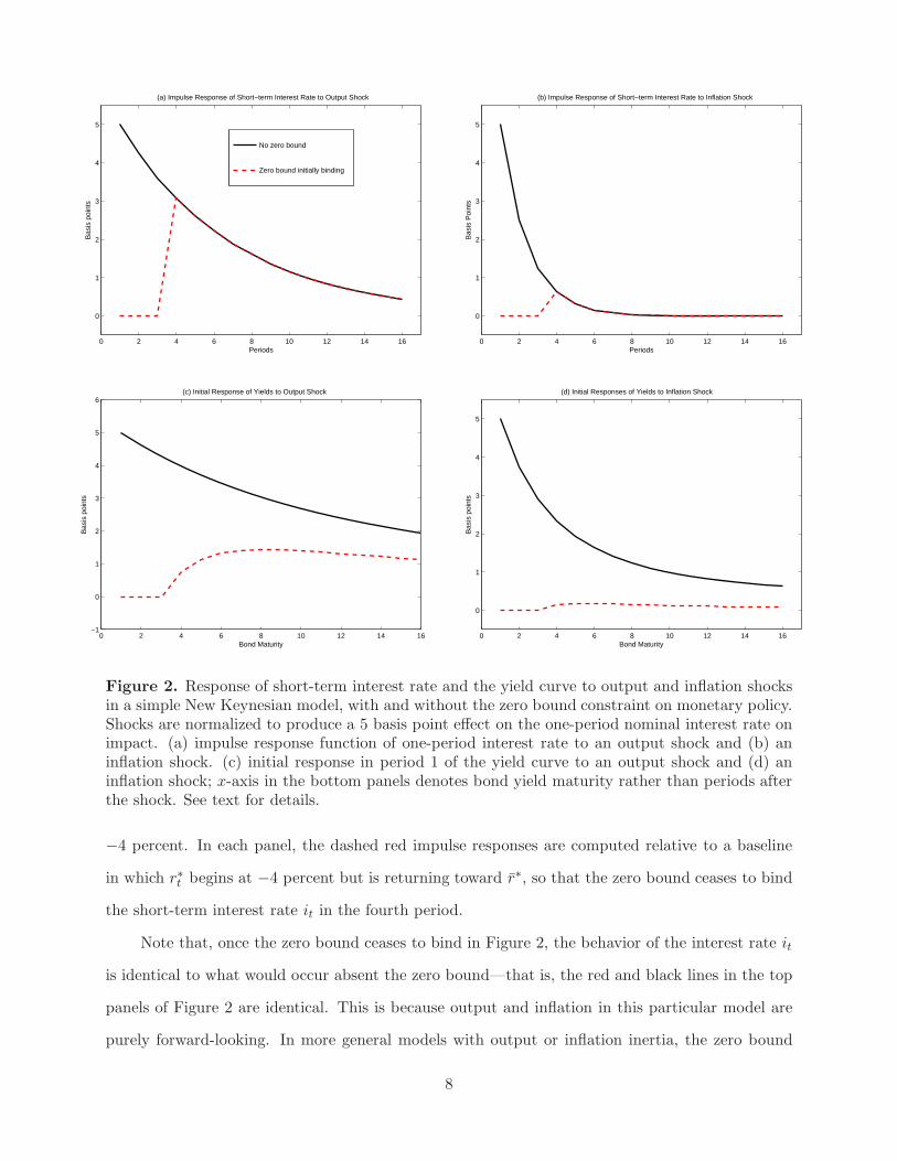
Figure 2. Response of short-term interest rate and the yield curve to output and inflation shocksin a simple New Keynesian model, with and without the zero bound constraint on monetary policy.Shocks are normalized to produce a 5 basis point effect on the one-period nominal interest rate onimpact. (a) impulse response function of one-period interest rate to an output shock and (b) aninflation shock. (c) initial response in period 1 of the yield curve to an output shock and (d) aninflation shock; x-axis in the bottom panels denotes bond yield maturity rather than periods afterthe shock. See text for details.

−4 percent. In each panel, the dashed red impulse responses are computed relative to a baseline

in which r∗t begins at −4 percent but is returning toward r∗, so that the zero bound ceases to bind

the short-term interest rate it in the fourth period.

Note that, once the zero bound ceases to bind in Figure 2, the behavior of the interest rate it

is identical to what would occur absent the zero bound—that is, the red and black lines in the top

panels of Figure 2 are identical. This is because output and inflation in this particular model are

purely forward-looking. In more general models with output or inflation inertia, the zero bound

8

would have more persistent effects on output and inflation, which would, in turn, lead to a more

persistent difference in the path of interest rates.

The bottom panels of Figure 2 depict the responses on impact of the yield curve to an output

or inflation shock in period 1, the period when the shock hits. Thus, the bottom panels of Figure 2

are not impulse response functions, but rather plot the instantaneous response of the entire yield

curve at a single point in time.

The first main point to take away from the model is that the response of the yield curve to

shocks is attenuated when the zero bound constrains policy, and the degree of attenuation declines

with the maturity of the bond. This can be seen clearly in the bottom panels of Figure 2. For the

shortest maturities, there is a total lack of responsiveness of the yield curve to an output or inflation

shock when the zero bound is binding, whereas for the longest-maturity bonds, the response of the

yield curve to an output or inflation shock becomes closer to the normal, unconstrained response.

Intermediate-maturity bonds are constrained by the zero bound to an intermediate extent. The

intuition for these results is clear and holds more generally than the simple illustrative model of

this section.

The second point to take away from the model is that the responses of yields to shocks are

essentially symmetric to positive and negative shocks. Figure 2 plots the response of the model

to small positive shocks, but the results for small negative shocks of the same size are exactly the

same in absolute value. This symmetry holds perfectly as long as the number of periods that policy

is constrained by the zero bound does not change, which is the case for small shocks.

Even for larger shocks, the responses of yields are essentially symmetric. Figure 3 plots the

absolute value of the impulse responses of the model to a positive (dashed red line) and negative

(solid blue line) output shock that are each ten times larger than in Figure 2 for the case where

the zero bound is binding. These are truly gigantic shocks, relative to the typical macroeconomic

data release surprise in our sample.9 Yet the two lines in the first panel of Figure 3 are still almost

9Recall from the previous footnote that the typical one-day response of Treasury yields to a single macroeconomicannouncement is only a few basis points. The shocks in Figure 3 are ten times as large as in Figure 2, and thusrepresent a roughly ten-standard-deviation surprise, so a one-day shock to yields of this magnitude is extremelyunlikely. Of course, over time, many small shocks can cumulate and gradually move the yield curve up or down bya larger amount, as discussed in Gurkaynak, Levin, and Swanson (2010). But from the point of view of a singlemacroeconomic data release, the results in Figures 2 and 3 and in our empirical tests, below, imply that the yieldcurve responses are almost perfectly symmetric.

9

0 2 4 6 8 10 12 14 16−5

0

5

10

15

20

25

30

35

Periods

Bas

is p

oint

s(a) Impulse Response of Short−term Interest Rate to Output Shock

Positive shockNegative shock (absolute value)

0 2 4 6 8 10 12 14 16−5

0

5

10

15

20(b) Initial Response of Yields to Output Shock

Bond Maturity

Bas

is p

oint

s

Figure 3. Absolute value of responses of short-term interest rate and yield curve to large positiveand negative output shocks in the simple New Keynesian model when the zero bound is binding.Shocks are normalized to produce a 50 bp effect on the one-period nominal interest rate on impact,ten times as large as in Figure 2. (a) impulse response function of one-period interest rate to theoutput shock; (b) initial response of the yield curve to an output shock. See text for details.

identical, except that the dashed red line lifts off from the zero bound one period sooner than the

blue line, because the positive shock increases policymakers’ desired interest rate above the zero

bound in that period. When the zero bound ceases to bind in either model in period 4, both

lines are identical for the same reasons as in Figure 2. The second panel of Figure 3 reports the

corresponding absolute value response of the yield curve on impact.

The fact that the zero bound causes the yield curve to be damped almost symmetrically to

positive and negative announcements can be counterintuitive at first, since the zero bound is a

one-sided constraint. Nevertheless, the intuition is clear and holds much more generally than in

just the simple model of this section: When the zero bound is a severe constraint on policy—that

is, policymakers would like to set the one-period nominal interest rate far below zero for several

periods—then short-term yields are completely unresponsive to both positive and negative shocks,

as long as those positive shocks are not large enough to bring short-term rates above the zero

bound. Longer-term yields are also about equally damped in response to positive and negative

shocks because: (a) longer-term yields are an average of current and expected future short-term

rates, (b) current short-term rates do not respond to either positive or negative shocks when the

zero bound is binding, and (c) expected future short-term rates respond symmetrically to positive

and negative shocks in periods in which the zero bound is not binding. There are very few periods in

10

which expected future short-term rates are unconstrained by the zero bound for the positive shock

but still constrained for the negative shock, and even in those periods the interest rate differential

between the two cases is typically small. These small differences are negligible compared to the

response of the yield curve as a whole, so the result is almost perfectly symmetric. We also test

this restriction in our empirical work below, and find that it is not rejected by the data.

The third and final point to take away from the model is that the dampening effects of the

zero bound on the sensitivity of yields is qualitatively the same regardless of the specific nature of

the shock, as can be seen in Figure 2. Moreover, the dampening effects are quantitatively similar

if the degree of persistence of the two shocks is similar. In Figure 2, the output shock was assumed

to be more persistent and continues to have large effects on interest rates in periods when the zero

bound is not binding; as a result, there is less dampening of the sensitivity of longer-term yields

in response to that shock. If the degree of persistence of the two shock processes were the same,

then the attenuation across maturities would be essentially identical for the output and inflation

shocks. In models with more complicated dynamics, the effects of the zero bound would differ

more substantially across the two types of shocks, but even in those models it remains true that

the degree of attenuation across maturities is determined primarily by the length of time the zero

lower bound is expected to bind, and not by the type of shock.

In our empirical work below, we assume that the zero bound attenuates the sensitivity of the

yield curve to news by the same amount for all shocks. In our theoretical model, this would only

be exactly true if all of the shocks had identical persistence characteristics in terms of their effects

on the short-term interest rate. Empirically, these persistences are unlikely to be exactly the same,

but we view this assumption as a reasonable approximation that can be tested, which we do below,

and find that it is not rejected by the data.

3 Empirical Framework

We now seek to estimate the extent to which Treasury securities of different maturities have been

more or less sensitive to macroeconomic announcements over time. We do this in three steps:

First, we identify the surprise component of major U.S. macroeconomic announcements. Second,

11

we estimate the average sensitivity of Treasury securities of each maturity to those announcements

over a benchmark sample, 1990–2000, during which the zero bound was not a constraint on yields.

Third, we compute the sensitivity of each Treasury yield in subsequent periods and compare it

to the benchmark sample to determine when and to what extent each yield was affected by the

presence of the zero lower bound. Periods in which the zero bound was a significant constraint on

a given Treasury yield should appear in this analysis as periods of unusually low sensitivity of that

security to macroeconomic news. We describe the details of each of these three basic steps in turn.

3.1 The Surprise Component of Macroeconomic Announcements

Financial markets are forward-looking, so the expected component of macroeconomic data releases

should have essentially no effect on interest rates.10 To measure the effects of these announcements

on interest rates, then, we first compute the unexpected, or surprise, component of each release.

As in Gurkaynak et al. (2005a), we compute the surprise component of each announcement

as the realized value of the macroeconomic data release on the day of the announcement less

the financial markets’ expectation for that realized value. We obtain data on financial market

expectations of major macroeconomic data releases from two sources: Money Market Services

(MMS) and Bloomberg Financial Services. Both MMS and Bloomberg conduct surveys of financial

market institutions and professional forecasters regarding their expectations for upcoming major

data releases, and we use the median survey response as our measure of the financial market

expectation. An important feature of these surveys is that they are conducted just a few days

prior to each announcement—historically, the MMS survey was conducted the Friday before each

data release, and the Bloomberg survey can be updated by participants until the night before the

release—so these forecasts should reflect essentially all relevant information up to a few days before

the release. Anderson et al. (2003) and other authors have verified that these data pass standard

tests of forecast rationality and provide a reasonable measure of ex ante expectations of the data

release, which we have verified over our sample as well.

Data from MMS for some macroeconomic series are available back to the mid-1980s, but are

only consistently available for a wider variety of series starting around mid-1989, so we begin our

10Kuttner (2001) tests and confirms this hypothesis for the case of monetary policy announcements.

12

sample on January 1, 1990. Bloomberg survey data begin in the mid-1990s but are available to us

more recently. When the two survey series overlap, they agree very closely, since they are surveying

essentially the same set of financial institutions and professional forecasters. Additional details

regarding these data are provided in Gurkaynak, Sack, and Swanson (2005a), Gurkaynak, Levin,

and Swanson (2010), and in Section 5.7, below.

3.2 The Sensitivity of Treasury Yields to Macroeconomic Announcements

In normal times, when Treasury yields are far away from the zero lower bound, those yields typically

respond to macroeconomic news. To measure this responsiveness, Gurkaynak et al. (2005a) estimate

daily-frequency regressions of the form

Δyt = α+ βXt + εt , (8)

where t indexes days, Δyt denotes the one-day change in the Treasury yield over the day, Xt is a

vector of surprise components of macroeconomic data releases that took place that day, and εt is a

residual representing the influence of other news and other factors on the Treasury yield that day.

Note that most macroeconomic data series, such as nonfarm payrolls or the consumer price index,

have data releases only once per month, so on days for which there is no news about a particular

macroeconomic series, we set the corresponding element of Xt equal to zero.11

Table 1 reports estimates of regression (8) for the 3-month, 2-year, and 10-year Treasury yields

from January 1990 through December 2000, a period in which we assume the zero lower bound

did not constrain these yields. We exclude days on which no major macroeconomic data releases

occurred, although the results are very similar whether or not these non-announcement days are

included. To facilitate interpretation of the coefficients in Table 1, each macroeconomic data release

surprise is normalized by its historical standard deviation, so that each coefficient in the table is in

units of basis points per standard-deviation surprise in the announcement.12

11Thus, if we write X as a matrix with columns corresponding to macroeconomic series and rows corresponding totime t, each column of X will be a vector consisting mostly of zeros, with one nonzero value per month correspondingto dates on which news about the corresponding macroeconomic series was released.

12The historical standard deviations of these surprises are as follows: capacity utilization, 0.34 percentage points;consumer confidence, 5.1 index points; core CPI, 0.11 percentage points; real GDP, 0.76 percentage points; initialclaims for unemployment insurance, 18.9 thousand workers; NAPM/ISM survey of manufacturers, 2.04 index points;leading indicators, 0.18 index points; new home sales, 60.6 thousand homes; nonfarm payrolls, 102.5 thousand workers;core PPI, 0.26 percentage points; retail sales excluding autos, 0.43 percentage points; and the unemployment rate,0.15 percentage points.

13

Treasury yield maturity

3-month 2-year 10-year

Capacity Utilization 1.68 (2.93) 2.10 (4.23) 1.47 (2.51)Consumer Confidence 0.29 (0.59) 2.67 (5.84) 2.69 (5.40)Core CPI 0.79 (2.55) 2.33 (4.38) 1.71 (3.38)GDP (advance) 0.33 (0.71) −0.18 (−0.19) −0.67 (−0.62)Initial Claims −0.29 (−1.36) −0.63 (−2.42) −0.39 (−1.43)ISM Manufacturing 0.98 (1.47) 3.44 (7.23) 2.61 (4.99)Leading Indicators 0.83 (1.58) 1.20 (2.36) 0.69 (1.09)New Home Sales 1.46 (3.56) 1.98 (4.84) 2.04 (4.30)Nonfarm Payrolls 2.44 (4.41) 4.56 (7.02) 2.86 (4.03)Core PPI 0.52 (1.40) 0.87 (1.78) 1.33 (2.60)Retail Sales ex. autos 1.19 (3.35) 1.83 (2.84) 1.18 (1.83)Unemployment rate −1.54 (−2.19) −1.98 (−2.60) −0.96 (−1.23)

# Observations 1303 1303 1303R2 .07 .19 .09H0 : β = 0, p-value < 10−8 < 10−16 < 10−16

Table 1. Coefficient estimates β from linear regression Δyt = α+ βXt + εt at daily frequency ondays of announcements from Jan. 1990 to Dec. 2000. Change in yields Δyt is in basis points; sur-prise component of macroeconomic announcements Xt are normalized by their historical standarddeviations; coefficients represent a basis point per standard deviation response. Heteroskedasticity-consistent t-statistics in parentheses. H0 : β = 0 p-value is for the test that all elements of β arezero. See text for details.

The first column of Table 1 reports results for the 3-month Treasury yield. Positive surprises

in output or inflation cause the 3-month Treasury yield to rise, on average, consistent with a Taylor-

type reaction function for monetary policy, while positive surprises in the unemployment rate or

initial jobless claims (which are countercyclical economic indicators) cause the 3-month Treasury

yield to fall. The data release that has the largest effect on 3-month Treasury yields is nonfarm

payrolls, for which a one-standard-deviation surprise causes yields to move by about 2.5 bp on

average, with a t-statistic of about 4.5. Taken together, the twelve data releases in Table 1 have a

highly statistically significant effect on the 3-month Treasury yield, with a joint F -statistic above

5 and a p-value of less than 10−8. The results for the 2- and 10-year Treasury yields in the second

and third columns are similar, with joint statistical significance levels that are even higher than for

the 3-month yield.13 Thus, the high-frequency types of regressions conducted in Table 1 provide

13The response of the 2-year Treasury yield to news is often larger than the response of the 3-month yield. In otherwords, the response of the yield curve to news tends to be hump-shaped. This is consistent with the standard resultin monetary policy VARs that the federal funds rate has a hump-shaped response to output and inflation shocks (e.g.,Sims and Zha 1999), and the finding in estimated monetary policy rules that the federal funds rate has inertia, sothat the central bank responds only gradually to news (e.g., Sack and Wieland 2000). For simplicity, we considered

14

a great deal of power and information with which to estimate time-variation in the sensitivity of

these yields to news in the next section.14

3.3 Measuring the Time-Varying Sensitivity of Treasury Yields

In principle, one can measure the time-varying sensitivity of Treasury yields to news by running

regressions of the form (8) over one-year rolling windows. However, this approach suffers from

small-sample problems because most macroeconomic series have data releases only once per month,

providing just twelve observations per year with which to identify each element of the vector β.

We overcome this small-sample problem by imposing that the relative magnitude of the ele-

ments of β are constant over time, so that only the overall magnitude of β varies as the yield in

question becomes more or less affected by the presence of the zero lower bound. Intuitively, if a

Treasury security’s sensitivity to news is reduced because its yield is starting to bump up against

the zero bound, then we expect that security’s responsiveness to all macroeconomic data releases

to be damped by a roughly proportionate amount. This assumption is supported by the illustrative

model in Section 2 and by empirical tests we conduct below.

Thus, for each given Treasury yield, we generalize regression (8) to a nonlinear least squares

specification of the form:

Δyt = γτi + δτiβXt + εt, (9)

where the parameters γτi and δτi are scalars that are allowed to take on different values in each

calendar year i = 1990, 1991, . . . , 2012. (The reason for the notation γτi , δτi rather than γi, δi will

become clear shortly.) The use of annual dummies in (9) is deliberately atheoretical in order to “let

the data speak” at this stage; we will consider higher-frequency and more structural specifications

a noninertial monetary policy rule in the previous section, but the key observations from that model are essentiallyunchanged if an inertial policy rule is used instead.

14Although the magnitudes of the coefficients in Table 1 are only a few basis points per standard deviation and theR2 less than 0.2, these results should not be too surprising given the low signal-to-noise ratio of any single monthlydata release for the true underlying state of economic activity and inflation. There are several reasons for this. Forone, our surprise data cover only the headline component of each announcement, while the full releases are muchricher: e.g., the employment report includes not just nonfarm payrolls and the unemployment rate, but also howmuch of the change in payrolls is due to government hiring, how much of the change in unemployment is due toworkers dropping out of the labor force, and revisions to the previous two nonfarm payrolls announcements. Thesituation is very similar for all of the other releases in Table 1, and details such as these typically have a substantialeffect on the markets’ overall interpretation of a release. The important point to take away from Table 1 is thatthe large number of observations and extraordinary statistical significance of the regressions implies that they areextremely informative about the sensitivity of Treasury yields to economic news.

15

for the time-varying sensitivity coefficients δ in this section and Section 5.6, below. Note that

regression (9) greatly reduces the small-sample problem associated with allowing every element of

β to vary across years, because in (9) there are about 140 observations of βXt per year with which

to estimate each scalar δτi . Regression (9) also brings about twice as much data to bear in the

estimation of β relative to the 1990–2000 sample considered in Table 1.

We must choose a normalization to separately identify the coefficients β and δτi in (9). We

normalize the δτi so that they have an average value of unity from 1990–2000, which we take to

be a period of relatively “normal” or unconstrained Treasury yield behavior. An estimated value

of δτi close to one thus represents a year in which the given Treasury yield behaved normally in

response to news, while an estimated value of δτi close to zero corresponds to a year in which the

given Treasury yield was completely unresponsive to news. Intermediate values of δτi correspond

to years in which the Treasury yield’s sensitivity to news was partially attenuated.

To provide a finer estimate of the periods during which each Treasury yield’s sensitivity was

attenuated, we also estimate daily rolling regressions of the form

Δyt = γτ + δτ Xt + ετt , (10)

where Xt ≡ βXt denotes a “generic surprise” regressor defined using the estimated value of β

from (9), and (10) is estimated over one-year rolling windows centered around each business day

τ from January 1990 through December 2012.15 When τ corresponds to the midpoint of a given

calendar year i ∈ {1990, 1991, . . . , 2012}, the estimated value of the attenuation coefficient δτ agrees

exactly with δτi from regression (9). But we can also estimate (10) for any business day τ in our

sample, and plot the coefficients δτ over time τ to provide a finer estimate of the periods during

which each Treasury yield’s sensitivity was attenuated. When we plot the standard errors in regres-

sion (10) around the point estimates for δτ , we account for the two-stage sampling uncertainty by

using the estimated standard errors of the δτi from regression (9) as benchmarks and interpolating

between them using the standard errors estimated in (10).

15Toward either end of our sample, the regression window gets truncated and thus becomes smaller and lesscentered, approaching a six-month leading window in January 1990 and a six-month trailing window in December2012.

16

Treasury yield maturity

3-month 2-year 10-year

Capacity Utilization 0.73 (1.56) 1.49 (2.89) 0.68 (2.02)Consumer Confidence 0.75 (2.90) 1.37 (3.71) 0.84 (2.43)Core CPI 0.39 (1.88) 1.89 (5.00) 1.17 (3.60)GDP (advance) 0.92 (3.15) 1.42 (2.40) 0.95 (1.69)Initial Claims −0.30 (−1.82) −1.10 (−5.35) −0.95 (−5.02)ISM Manufacturing 1.23 (3.24) 2.72 (7.09) 1.98 (5.96)Leading Indicators 0.20 (0.62) 0.28 (0.85) 0.28 (1.01)New Home Sales 0.83 (2.65) 0.65 (1.99) 0.50 (1.93)Nonfarm Payrolls 3.03 (7.67) 4.79 (9.54) 2.95 (6.79)Core PPI 0.22 (0.79) 0.52 (1.54) 0.85 (3.14)Retail Sales ex. autos 0.83 (3.76) 1.86 (4.92) 1.62 (4.31)Unemployment rate −1.24 (−3.53) −1.26 (−2.78) −0.41 (−1.07)

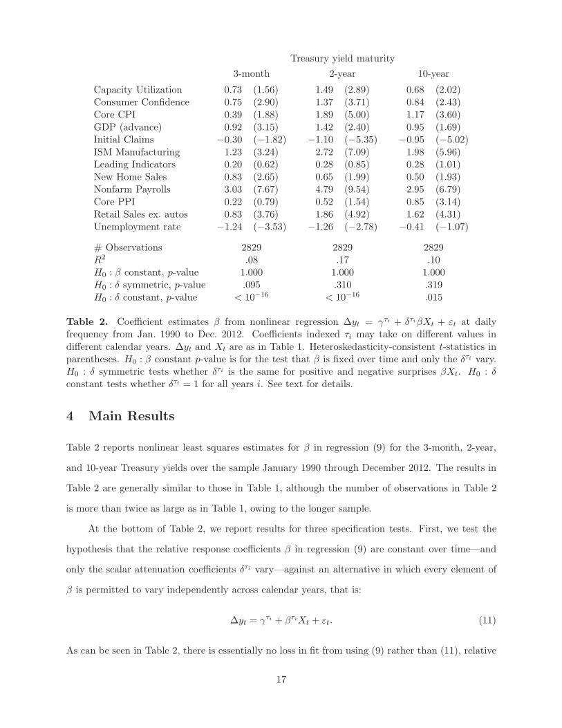
# Observations 2829 2829 2829R2 .08 .17 .10H0 : β constant, p-value 1.000 1.000 1.000H0 : δ symmetric, p-value .095 .310 .319H0 : δ constant, p-value < 10−16 < 10−16 .015

Table 2. Coefficient estimates β from nonlinear regression Δyt = γτi + δτiβXt + εt at dailyfrequency from Jan. 1990 to Dec. 2012. Coefficients indexed τi may take on different values indifferent calendar years. Δyt and Xt are as in Table 1. Heteroskedasticity-consistent t-statistics inparentheses. H0 : β constant p-value is for the test that β is fixed over time and only the δτi vary.H0 : δ symmetric tests whether δτi is the same for positive and negative surprises βXt. H0 : δconstant tests whether δτi = 1 for all years i. See text for details.

4 Main Results

Table 2 reports nonlinear least squares estimates for β in regression (9) for the 3-month, 2-year,

and 10-year Treasury yields over the sample January 1990 through December 2012. The results in

Table 2 are generally similar to those in Table 1, although the number of observations in Table 2

is more than twice as large as in Table 1, owing to the longer sample.

At the bottom of Table 2, we report results for three specification tests. First, we test the

hypothesis that the relative response coefficients β in regression (9) are constant over time—and

only the scalar attenuation coefficients δτi vary—against an alternative in which every element of

β is permitted to vary independently across calendar years, that is:

Δyt = γτi + βτiXt + εt. (11)

As can be seen in Table 2, there is essentially no loss in fit from using (9) rather than (11), relative

17

to the degrees of freedom of the restriction: the p-values are equal to 1 to at least three decimal

places. The assumption of a constant β in (9) is thus very consistent with the data.

Second, we test the hypothesis that the δτi in (9) are the same for positive and negative

surprises βXt, against an alternative in which we allow separate attenuation coefficients δτi+ and δτi−

for positive and negative values of βXt in each calendar year i. In other words, we separate the

data into two groups—those announcements that have positive implications for Treasury yields,

and those that have negative implications—and test whether the attenuation coefficients δτi+ = δτi−

for each i = 1990, . . . , 2012.16 As can be seen in Table 2, this restriction is also not rejected by the

data, with p-values typically substantially above ten percent. Although the symmetry restriction

appears to be marginally rejected for the 3-month Treasury yield, with a p-value of .095, that result

is entirely driven by a large outlier on October 20, 2008, when the 3-month T-bill yield jumped by

41 bp.17 Excluding that single observation, the p-value for the 3-month Treasury yield hypothesis

test is .709. We conclude that this restriction is also consistent with the data.

Third, we test the hypothesis that the time-varying sensitivity coefficients δτi in (9) are con-

stant over time. That is, we test whether δτi = 1 for each calendar year i = 1990, . . . , 2012. In

contrast to the previous two tests, here the data strongly reject the restriction for the 3-month and

2-year Treasury yields, with p-values less than 10−16. Clearly, the sensitivity of these two yields to

macroeconomic news has varied substantially over time. The constant-δ restriction for the 10-year

yield is also rejected, but less strongly, with a p-value of .015. Although the 10-year yield’s sensi-

tivity to news does appear to have varied over time, the assumption of constant sensitivity for this

yield is not nearly as inconsistent with the data as for the shorter-maturity yields.

Figure 4 plots the time-varying sensitivity coefficients δτ from regression (9) as a function of

time τ , using the daily rolling regression specification (10). The six panels of the figure depict

results for the 3-month, 6-month, and 1-, 2-, 5-, and 10-year Treasury yields. The solid blue

16The first group consists of all of the unemployment rate and initial claims surprises that are less than zero, andall of the positive surprises in the other statistics. The second group consists of all of the unemployment rate andinitial claims surprises that are greater than zero, and all of the negative surprises in the other statistics.

17The only macroeconomic data released that day was leading indicators, which had a positive surprise of about2 standard deviations. According to The Wall Street Journal, the major news that day was that J.P. MorganChase and other large banks lent billions of dollars to their counterparts in Europe, which “spurred improvementin the commercial paper market. . .With more appetite for risk came an exodus out of government debt. Treasurybills suffered the most. . . Bills were also pressured by more than $80 billion in bill supply. . . from the Treasurydepartment.” (“Credit Markets: Bonds and Stocks Show Signs of Healing,” The Wall Street Journal, October 21,2008, Romy Varghese and Emily Barrett, p. C1.)

18

line in each panel plots the estimated value of δτ on each date τ , while the dotted gray lines

depict heteroskedasticity-consistent ±2-standard-error bands, adjusted for the two-stage estimation

procedure as described in the preceding section. In each panel, horizontal black lines are drawn

at 0 and 1 as benchmarks for comparison, corresponding to the cases of complete insensitivity to

news and normal sensitivity to news, respectively.

In each panel, the yellow shaded regions denote periods during which the estimated value

of δτ is significantly less than unity at the one percent level. We use a conservative threshold

here so that the shaded regions represent periods in which the yield was clearly less sensitive to

news than normal. In addition, if the hypothesis δτ = 0 cannot be rejected, then the region is

shaded red.18 Thus, red shaded regions correspond to periods in which the Treasury yield was

essentially insensitive to news, while yellow shaded regions correspond to periods in which the yield

was partially—but not completely—unresponsive to news.

Panel (a) of Figure 4 shows that the sensitivity of the 3-month Treasury yield to macroecon-

omic news has varied between about 0 and 2 from 2001 through 2012. From the spring of 2009

through the end of 2012, the 3-month Treasury yield was either partially or completely insensitive

to news. It is natural to interpret this insensitivity as being driven by the zero lower bound, since

the federal funds rate and 3-month Treasury yields were both essentially zero from December 2008

through the end of our sample. At the shortest end of the yield curve, at least, Treasury yields

appear to have been substantially constrained by the zero bound from the spring of 2009 onward.

What is perhaps more surprising in the first panel of Figure 4 is that the 3-month Treasury

yield was also partially or completely insensitive to news throughout 2003 and 2004, a period

during which the federal funds rate target and 3-month Treasury yield never fell below 1 percent.

However, the Fed had recently lowered the funds rate to 1.25 percent in November 2002 and again

to 1 percent in June 2003, and at the time, a level of the funds rate below 1 percent was regarded as

costly for institutional reasons (Bernanke and Reinhart, 2004). Rather than try to lower the funds

rate below 1 percent, the FOMC opted instead to switch to a policy of managing monetary policy

expectations, using phrases such as “policy accommodation can be maintained for a considerable

18We use a standard five percent threshold here. A one percent threshold would result in the red shaded regionsbeing slightly larger.

19

2002 2004 2006 2008 2010 2012

-1

-0.5

0

0.5

1

1.5

2

2.5

3

3.5

4

(a) 3-Month Treasury Yield Sensitivity to News

2002 2004 2006 2008 2010 2012-1

-0.5

0

0.5

1

1.5

2

2.5

3

3.5

4(b) 6-Month Treasury Yield Sensitivity to News

2002 2004 2006 2008 2010 2012-1

-0.5

0

0.5

1

1.5

2

2.5

3

3.5

4(c) 1-Year Treasury Yield Sensitivity to News

2002 2004 2006 2008 2010 2012-1

-0.5

0

0.5

1

1.5

2

2.5

3

3.5

4(d) 2-Year Treasury Yield Sensitivity to News

2002 2004 2006 2008 2010 2012-1

-0.5

0

0.5

1

1.5

2

2.5

3

3.5

4(e) 5-Year Treasury Yield Sensitivity to News

2002 2004 2006 2008 2010 2012

-1

-0.5

0

0.5

1

1.5

2

2.5

3

3.5

4

(f) 10-Year Treasury Yield Sensitivity to News

Figure 4. Time-varying sensitivity coefficients δτ from regression (10) for (a) 3-month, (b) 6-month, (c)1-year, (d) 2-year, (e) 5-year, and (f) 10-year Treasury yields. Dotted gray lines depict heteroskedasticity-consistent ±2-standard-error bands, adjusted for two-stage sampling uncertainty in (10). δτ = 1 corre-sponds to normal Treasury sensitivity to news; δτ = 0 to complete insensitivity. Yellow shaded regionsdenote δτ significantly less than 1; red shaded regions denote δτ significantly less than 1 and not signifi-cantly different from 0. See text for details. 20

period.”19 Thus, even though the funds rate was not constrained by a floor of zero in 2003 and

2004, our results show that the 3-month Treasury yield behaved as if it had been constrained by a

floor of 1 percent. The fact that our empirical method picks up the constraints faced by monetary

policy in 2003–04, and the potential absence of crowding out of fiscal policy over the same period,

is a noteworthy feature of our approach.

Panel (b) of Figure 4 reports analogous results for the 6-month Treasury yield, which are

generally similar to those for the 3-month yield: the sensitivity to macroeconomic news ranges

between 0 and 2, and from the spring of 2009 through the end of 2012, the 6-month yield was

either partially or completely unresponsive to news. In contrast to the 3-month yield, however, the

6-month yield’s sensitivity to news was much less attenuated in 2003–04. Thus, to the extent that

the effective lower bound of 1 percent was a substantial constraint on monetary policy in 2003–04,

that constraint did not appear to extend out to maturities beyond 3 months in 2004.

Results for 1- and 2-year Treasury yields are reported in the middle panels of Figure 4. The

sensitivity of these intermediate-maturity yields to news is less attenuated than that of 3- and

6-month yields throughout our sample. For example, both the 1- and 2-year yields behaved close

to normally throughout 2003–04, implying that they were relatively unaffected by the FOMC’s

implicit floor of about 1 percent during this period. Thus, to the extent that the FOMC can affect

yields with a year or more to maturity, we would conclude that the effectiveness of monetary and

fiscal policy were very close to normal in 2003–04.

What is perhaps most surprising in the middle panels of Figure 4 is how little and how late the

zero bound seems to have affected these intermediate-maturity yields after 2008. The sensitivity of

the 1-year yield to news was only significantly less than unity beginning in 2010, and even then is

partially responsive to news until late 2011. Only beginning in late 2011 does the 1-year Treasury

yield cease responding to news. The 2-year Treasury yield’s sensitivity to news was generally not

significantly attenuated until late 2011, and even then remained partially responsive to news until

late 2012. Thus, to the extent that the Fed can influence monetary policy expectations over a

horizon out to two years, we conclude that monetary and fiscal policy were about as effective as

19The “considerable period” language was introduced into the FOMC statement on August 12, 2003, and continueduntil the end of January 2004, at which point it was replaced with the phrase, “the Committee believes that it canbe patient in removing its policy accommodation.” The funds rate was finally raised on June 30, 2004.

21

usual until at least late 2011.

The bottom two panels of Figure 4 report results for 5- and 10-year Treasury yields, which are

also remarkable. There are essentially no red or yellow shaded regions in these panels, because the

sensitivity of these yields to news is never significantly less than one until the last few weeks of 2012.

Even in late 2011 and 2012, when Treasury yields out to two years were becoming substantially

constrained, 5- and 10-year yields remained largely unconstrained. However, the sensitivity of the

5-year yield to news declined throughout 2012, and given the substantial decline in the 5- and

10-year yields’ sensitivity to news toward the end of 2012, it would be very interesting to see how

this sensitivity evolves going forward.

5 Discussion

We now discuss the broader implications of our empirical results and perform several extensions

and robustness checks. First, we compare our results to private-sector expectations of the time

until federal funds rate “liftoff” from the zero bound. Second, we provide evidence that the Federal

Reserve can manage monetary policy expectations at horizons out to several quarters. Third, we

relate our results to the Federal Reserve’s large-scale purchases of long-term bonds. Fourth, we

discuss the implications of our findings for the fiscal multiplier. Fifth, we consider the differences

between an exogenous zero lower bound constraint and a voluntary commitment by the central

bank to a policy path. Sixth, we investigate to what extent a reduced sensitivity of Treasury

yields to news can be explained mechanically by a lower level of yields or by changes in monetary

policy uncertainty. Finally, we show that the distribution of our macroeconomic surprise data from

2008–12 is not very different from the distribution of those surprises before 2008.

5.1 Private-Sector Expectations of Federal Funds Rate “Liftoff” from Zero

Our illustrative model in Section 2 implies that the sensitivity of medium- and longer-term Treasury

yields to news is closely related to the length of time that the federal funds rate is expected to

be at the zero lower bound. For example, if the funds rate is expected to be at zero for just

one quarter, then medium- and longer-term interest rates should be nearly unaffected by the zero

22

0

1

2

3

4

5

6

7

Quarters

or more

FOMC issues"mid-2013" guidance

Figure 5. Expected number of quarters until the first federal funds rate increase above 25 bp,from the monthly Blue Chip survey of forecasters. Data are top-coded at “7 or more” quarters dueto the forecast horizon length published by Blue Chip.

bound, whereas if the funds rate is expected to be at the zero bound for several years, then even

5- or 10-year Treasury yields should be noticeably affected.

Figure 5 plots the number of quarters until the private sector expected the funds rate to be

25 bp or higher, as measured by the median, “consensus” response to the monthly Blue Chip survey

of professional forecasters. Prior to December 2008, the FOMC was not expected to lower the funds

rate below 25 bp for any length of time. After the FOMC cut the target funds rate to near zero

in December 2008, the Blue Chip consensus expectation of the length of time until the first funds

rate increase then fluctuated between two and five quarters until August 2011. On August 9, 2011,

the FOMC announced that it expected to keep the funds rate at zero until at least “mid-2013,”

and private-sector expectations of the time until liftoff jumped to seven or more quarters (the Blue

Chip forecast horizon extends forward only six quarters).20

The implication of the forecasts underlying Figure 5 is that, from about January 2009 until

20The Federal Reserve Bank of New York also surveys primary dealers in the Treasury market, with survey resultssince January 2011 made available at http://www.newyorkfed.org/markets/primarydealer survey questions.html.The results of this survey show a similar jump in the median primary dealer forecast, from 5 quarters in August 2011to 9 quarters in September 2011.

23

Jan 2008 Oct 2008 Jun 2009 Mar 2010 Dec 2010 Aug 2011 May 2012 Jan 20130

0.1

0.2

0.3

0.4

0.5

0.6

0.7

0.8

0.9

1

Figure 6. Probability the federal funds rate would be less than 50 bp in five quarters, estimatedfrom options data. See text for details.

August 2011, the sensitivity of Treasury yields with a year or less to maturity should have fallen close

to zero, while that for maturities of two years or more should have been only partially attenuated.

Only beginning in August 2011 would we expect to see yields with two years to maturity show a

more substantial attenuation with respect to news. And in fact, this corresponds closely to our

time-varying sensitivity results in Figure 4.

Figure 6 provides an additional perspective on these results from the interest rate options

market. Using daily options data with a range of strike prices and five quarters to expiration, we

can estimate the entire implied distribution of the federal funds rate in five quarters’ time at daily

frequency.21 We can then use these estimated distributions to back out the implied probability that

the federal funds rate would be less than 50 bp in five quarters’ time, which we plot in Figure 6

from January 2008 to December 2012.

21We do not need to assume normality for these distributions because we observe option prices for multiple differentstrikes. On each day from January 2008 through December 2012, we use the range of available Eurodollar option putand call prices with five quarters to expiration to estimate the implied distribution of the spot 3-month Eurodollarrate in five quarters’ time, using a flexible functional form. Eurodollar options are the most liquid options on a short-term interest rate and thus provide the best measure of the distribution of possible short-term interest rate outcomes.We use the spread between overlapping federal funds futures and Eurodollar futures rates at a one-year horizon toconvert these implied distributions for the 3-month Eurodollar rate into an implied distribution for the federal fundsrate. These probability estimates ignore risk premia and thus represent implied risk-neutral probabilities.

24

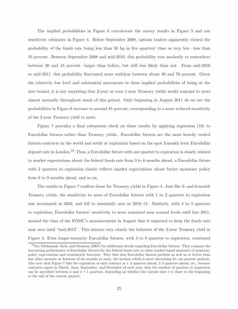
The implied probabilities in Figure 6 corroborate the survey results in Figure 5 and our

sensitivity estimates in Figure 4. Before September 2008, options traders apparently viewed the

probability of the funds rate being less than 50 bp in five quarters’ time as very low—less than

10 percent. Between September 2008 and mid-2010, this probability rose modestly to somewhere

between 20 and 45 percent—larger than before, but still less likely than not. From mid-2010

to mid-2011, this probability fluctuated more widelym between about 30 and 70 percent. Given

the relatively low level and substantial movements in these implied probabilities of being at the

zero bound, it is not surprising that 2-year or even 1-year Treasury yields would respond to news

almost normally throughout much of this period. Only beginning in August 2011 do we see the

probabilities in Figure 6 increase to around 85 percent, corresponding to a more reduced sensitivity

of the 2-year Treasury yield to news.

Figure 7 provides a final robustness check on these results by applying regression (10) to

Eurodollar futures rather than Treasury yields. Eurodollar futures are the most heavily traded

futures contracts in the world and settle at expiration based on the spot 3-month term Eurodollar

deposit rate in London.22 Thus, a Eurodollar future with one quarter to expiration is closely related

to market expectations about the federal funds rate from 3 to 6 months ahead, a Eurodollar future

with 2 quarters to expiration closely reflects market expectations about future monetary policy

from 6 to 9 months ahead, and so on.

The results in Figure 7 confirm those for Treasury yields in Figure 4. Just like 3- and 6-month

Treasury yields, the sensitivity to news of Eurodollar futures with 1 to 2 quarters to expiration

was attenuated in 2003, and fell to essentially zero in 2010–12. Similarly, with 4 to 5 quarters

to expiration, Eurodollar futures’ sensitivity to news remained near normal levels until late 2011,

around the time of the FOMC’s announcement in August that it expected to keep the funds rate

near zero until “mid-2013”. This mirrors very closely the behavior of the 2-year Treasury yield in

Figure 4. Even longer-maturity Eurodollar futures, with 5 to 8 quarters to expiration, continued

22See Gurkaynak, Sack, and Swanson (2007) for additional details regarding Eurodollar futures. They compare theforecasting performance of Eurodollar futures for the federal funds rate to other market-based measures of monetarypolicy expectations and econometric forecasts. They find that Eurodollar futures perform as well as or better thanany other measure at horizons of six months or more, the horizon which is most interesting for our present analysis.Also note that Figure 7 lists the expiration of each contract as 1–2 quarters ahead, 2–3 quarters ahead, etc., becausecontracts expire in March, June, September, and December of each year; thus the number of quarters to expirationcan lie anywhere between n and n + 1 quarters, depending on whether the current date t is closer to the beginningor the end of the current quarter.

25

2002 2004 2006 2008 2010 2012-0.5

0

0.5

1

1.5

2

2.5

3

3.5

4(a) 1 to 2-Quarter-Ahead Eurodollar Future Sensitivity to News

2002 2004 2006 2008 2010 2012-0.5

0

0.5

1

1.5

2

2.5

3

3.5

4(b) 2 to 3-Quarter-Ahead Eurodollar Future Sensitivity to News

2002 2004 2006 2008 2010 2012-0.5

0

0.5

1

1.5

2

2.5

3

3.5

4(c) 3 to 4-Quarter-Ahead Eurodollar Future Sensitivity to News

2002 2004 2006 2008 2010 2012-0.5

0

0.5

1

1.5

2

2.5

3

3.5

4(d) 4 to 5-Quarter-Ahead Eurodollar Future Sensitivity to News

2002 2004 2006 2008 2010 2012-0.5

0

0.5

1

1.5

2

2.5

3

3.5

4(e) 5 to 6-Quarter-Ahead Eurodollar Future Sensitivity to News

2002 2004 2006 2008 2010 2012

-0.5

0

0.5

1

1.5

2

2.5

3

3.5

4

(f) 7 to 8-Quarter-Ahead Eurodollar Future Sensitivity to News

Figure 7. Time-varying sensitivity coefficients δτ from regression (10) for Eurodollar futures contractswith (a) 1–2 quarters, (b) 2–3 quarters, (c) 3–4 quarters, (d) 4–5 quarters, (e) 5–6 quarters, and (f) 7–8quarters to expiration. Eurodollar futures settle based on the spot 3-month Eurodollar deposit rate atexpiration, and thus correspond to forward interest rates beginning at expiration and ending 1 quarterafter expiration. See notes to Figure 4 and text for details.

26

to respond normally to news until the FOMC announced in January 2012 that it expected to keep

the funds rate near zero until “late 2014”.

Like the Blue Chip survey data and options data, these results corroborate our findings for

Treasury yields and suggest that financial markets did not expect the zero bound to constrain the

federal funds rate for more than a few quarters until about August 2011. Only then do we see

interest rate expectations more than four quarters ahead begin to behave in an attenuated fashion.

5.2 Can the Fed Manage Monetary Policy Expectations?

Our findings above suggest that interest rate expectations more than a few quarters ahead were

largely unaffected by the zero bound until at least August 2011. Thus, even though the federal funds

rate was severely constrained by the zero lower bound beginning in December 2008, monetary policy

more broadly defined might not have been substantially constrained to the extent that the Federal

Reserve can affect monetary policy expectations. In this section, we briefly review the evidence

on the Federal Reserve’s ability to influence these expectations without changing the current level

of the federal funds rate. Note that, even if the Fed had no ability to influence monetary policy

expectations, our findings above would still have interesting implications for fiscal policy and the

degree to which fiscal stimulus crowded out private-sector investment.

In theory, a central bank can influence private-sector expectations of future monetary policy

if the bank has some ability to at least partially commit to its future policy actions. Schaumburg

and Tambalotti (2007) and Debortoli and Nunes (2010) define a continuum of partial commitment

technologies that lie between perfect commitment and perfect discretion, in the sense of Kydland

and Prescott (1977). Since perfect discretion is a limiting case along this continuum and implies

no ability to commit whatsoever, it seems likely—or at least possible—that monetary policymakers

would have some ability to influence private-sector expectations of future monetary policy actions

at least a few periods ahead. Nevertheless, the Federal Reserve’s ability to manipulate expectations

about monetary policy several quarters into the future is ultimately an empirical question.

Empirically, there are several studies of the Federal Reserve’s ability to influence longer-term

interest rates through its communications, such as through the statements released by the FOMC

after each monetary policy meeting. Gurkaynak, Sack, and Swanson (2005b) separately identify

27

Treasury yields

3-month 6-month 1-year 2-year 5-year 10-year

FOMC drops “considerable period” language on Jan. 28, 2004

Jan. 27, 2004 0.91 0.98 1.17 1.694 3.082 4.391Jan. 28, 2004 0.94 1.00 1.295 1.86 3.221 4.494change (bp) 3 2 12.5 16.6 13.9 10.3

FOMC projects zero funds rate “at least through mid-2013” on Aug. 9, 2011

Aug. 8, 2011 0.05 0.07 0.173 0.271 1.133 2.591Aug. 9, 2011 0.03 0.06 0.13 0.172 0.928 2.362change (bp) −2 −1 −4.3 −9.9 −20.5 −22.9

Table 3. Response of Treasury yields to significant changes in FOMC statements on Jan. 28, 2004,and Aug. 9, 2011. In both cases, there was no change in the current federal funds rate target, butthe statement described a substantial change in the outlook for the funds rate relative to marketexpectations. See text for details.

the impact of FOMC actions (changes in the federal funds rate target) and statements, and find

that FOMC statements have highly statistically significant effects on Treasury yields out to matu-

rities of 10 years. In fact, more than half of the explainable variation in the response of two-year

Treasury yields (and almost 90 percent of the variation in the response of 10-year yields) to FOMC

announcements is attributable to the FOMC’s statements, rather than to changes in the current

federal funds rate target. The authors’ interpretation of this finding is not that statements have

some mysterious independent power over longer-term interest rates, but rather that statements

affect longer-term yields by changing financial market expectations about the future path of the

funds rate. Bernanke, Reinhart, and Sack (2004) review these results and come to very similar

conclusions using slightly different methods.23 More recently, Campbell et al. (2012) extend the

Gurkaynak et al. (2005b) analysis through the end of 2011, and find that the FOMC’s statements

continued to have similarly large effects on longer-term bond yields throughout the financial crisis

and its aftermath in 2007–11.

Table 3 highlights two examples of this effect. From August 2003 until January 2004, the

FOMC stated after each of its meetings that the accommodative stance of monetary policy “can

be maintained for a considerable period.” On January 28, 2004, in response to the strengthening

economic outlook, the FOMC dropped this phrase from its statement and replaced it with the

23Kohn and Sack (2004) also find that FOMC statements and Congressional testimony by the Fed Chairman havesignificant effects on longer-term interest rates, and present evidence that changes in monetary policy expectationsare the primary driver of these changes.

28

phrase “the Committee believes it can be patient in removing its policy accommodation.”24 Even

though the funds rate target itself was unchanged on that date, the change in the statement was read

by financial markets as indicating that the FOMC would begin raising the funds rate sooner than

previously expected.25 The result was that longer-term Treasury yields responded dramatically to

the announcement, rising by about 10 to 16 bp at maturities of one to ten years. Note that, in

normal times, it would take a surprise cut in the federal funds rate of about 100 bp to generate a

decline of this size in intermediate-maturity yields (Gurkaynak et al. 2005b).

Similarly, on August 9, 2011, in response to the weakening economic outlook, the FOMC

announced that “economic conditions. . . are likely to warrant exceptionally low levels for the federal

funds rate at least through mid-2013.” Because the federal funds rate was already at an effective

lower bound of 0 to 25 bp, there was no change in the FOMC’s current federal funds rate target.

Analogous to the previous example, financial markets read the change in statement as signaling

the FOMC would likely begin raising the funds rate later than previously expected.26 As a result,

longer-term Treasury yields fell substantially, about 10 to 23 bp at maturities of two to ten years.

The Blue Chip survey evidence presented in Figure 5 also suggests that this announcement had a

large effect on monetary policy expectations.

These two examples are representative of the more comprehensive and systematic evidence

in the studies cited above. These studies suggest that the FOMC does have the ability to influ-

ence monetary policy expectations for at least the next few years, and thereby affect the level of

intermediate-maturity Treasury yields and Eurodollar futures with several quarters to expiration.

5.3 The Federal Reserve’s Purchases of Long-Term Bonds

The Federal Reserve may also be able to influence longer-term interest rates by changing the sup-

ply of long-term bonds available to the private sector through large-scale open-market purchases.

Although standard representative-agent asset pricing models do not allow for the quantity of a

24The statements released after each FOMC meeting are available from the Federal Reserve Board’s web site.25For example, the front page of The Wall Street Journal reported the following morning that “investors interpreted

the omission of ‘considerable period’ as a signal that the Fed is closer to raising rates than many thought.” (“FedClears Way for Future Rise in Interest Rates,” The Wall Street Journal, Jan. 29, 2004, Greg Ip, p. A1.)

26The front page of The Wall Street Journal the following morning noted that, in response to the FOMC statement,financial markets “lowered their expectations for when the Fed will start tightening policy.” (“Markets Sink ThenSoar after Fed Speaks,” The Wall Street Journal, Aug. 10, 2011, Sudeep Reddy and Jonathan Cheng, p. A1.)

29

security to have any effect on its price, Vayanos and Vila (2009) provide a modern, arbitrage-free

foundation for the earlier “portfolio balance” and “preferred habitat” models of Tobin (1958) and

Modigliani and Sutch (1966).27 Intuitively, if private-sector investors have heterogeneous prefer-

ences for different bond maturities, and arbitrage across maturities is limited, then the supply of

longer-term bonds in the market can affect longer-term bond yields.

Empirically, Bernanke et al. (2004), Krishnamurthy and Vissing-Jorgensen (2011, 2012), Gagnon

et al. (2011), Swanson (2011), and others find that large changes in the supply of Treasury securities

have had appreciable effects on the yields of those securities. Between 2008 and 2012, the FOMC

announced several rounds of large-scale purchases of longer-term Treasury and agency-backed secu-

rities, amounting to over $3.2 trillion in total.28 These purchases represented a substantial fraction

of the quantity of longer-term Treasury bonds in the hands of the private sector (Gagnon et al.

2011), and thus would be expected to have appreciable effects on longer-term bond yields based on

the findings of the studies cited above.

Indeed, these purchases may help to explain a surprising feature of our results in Figure 4,

namely that 10-year and, to some extent, 5-year Treasury yields were no less sensitive to news

between 2008 and 2012 than in normal times. On the one hand, a finding of relatively little

attenuation in the sensitivity of longer-term yields before August 2011 is not surprising, given how

quickly market participants expected the funds rate to lift off from zero. But the continued lack of

attenuation for 5- and 10-year Treasuries in late 2011 and 2012 is surprising, given that the 2-year

yield’s sensitivity to news had fallen so far by that time.

A possible explanation for this finding is that market participants expected the Fed to adjust

its purchases of long-term bonds in response to changing economic conditions. Since the studies

27See also Hamilton and Wu (2012), who relate the Vayanos-Vila model to a standard arbitrage-free affine termstructure model to estimate quantity effects.

28On November 25, 2008, the FOMC announced that it would purchase $500 billion of mortgage-backed securitiesand $100 billion of debt directly issued by the housing-related government-sponsored enterprises (GSEs); on March 18,2009, the FOMC announced it would purchase an additional $750 billion of mortgage-backed securities, an additional$100 billion of GSE debt, and $300 billion of longer-term Treasury securities; on November 3, 2010, the FOMCannounced that it would purchase an additional $600 billion of longer-term Treasury securities; on September 21,2011, the FOMC announced it would exchange an additional $400 billion of short-term Treasury securities for anequal amount of long-term Treasury bonds, which did not increase the FOMC’s total holdings of Treasury securitiesbut substantially altered the composition of those holdings; on June 20, 2012, the FOMC announced an extension ofthe September 2011 program, amounting to an additional $270 billion of long-term bond purchases; on September 13,2012, the FOMC announced it would purchase an additional $40 billion per month of mortgage-backed securities forthe indefinite future; and on December 12, 2012, the FOMC announced it would continue purchasing an additional$45 billion per month of longer-term Treasury securities for the indefinite future.

30

cited above found these purchases have substantial effects on longer-term yields, this could have

offset any dampening effect from the zero bound on those yields. The net result would be less

attenuation in the sensitivity of 5- and 10-year Treasury yields to news between 2008 and 2012,

perhaps even resulting in no net attenuation, as we found in Figure 4.

5.4 Implications for the Fiscal Multiplier

Our empirical results also have important implications for the growing literature on the fiscal

multiplier at the zero lower bound (e.g., Christiano et al. 2011, Woodford 2011).29 An important

finding of that literature is that the fiscal multiplier is larger the greater the fraction of the change

in government spending that is expected to take place while the short-term interest rate is at zero.30

Put differently, for a given path of fiscal stimulus, the multiplier is larger the longer the zero lower

bound is expected to constrain the short-term interest rate.

Figure 8 illustrates two possible scenarios for the expected path of short-term interest rates.

In scenario A (the red line), the short-term rate is expected to lift off from the zero bound relatively

quickly, at time tA. In scenario B (the blue line), the short-term rate is expected to lift off later,

at tB > tA. According to the analysis in Woodford (2011) and Christiano et al. (2011, henceforth

CER), for a given increase or decrease in the expected path of government purchases between

time 0 and tB , the fiscal multiplier is larger in scenario B than in scenario A, for two reasons.

First, in scenario B a greater fraction of the change in government purchases takes place while the

short-term interest rate is zero, which increases the fiscal multiplier. Second, in scenario B the zero

lower bound is expected to bind for a longer period of time, which by itself also increases the fiscal

multiplier, as discussed by those authors.

Our empirical results shed light on the relative plausibility of different scenarios such as A and

B in Figure 8. In particular, our findings suggest that financial markets in 2008–10 expected the

29See also Eggertsson (2009), Erceg and Linde (2010), Eggertsson and Krugman (2012), and DeLong and Summers(2012).

30For example, “Our basic result is that the multipliers are higher the larger the percentage of the spending thatcomes on line when the nominal interest rate is zero” (Christiano et al. 2011, p. 112). “Hence, while there is apositive effect on output during the crisis of increased government purchases at date t < T , an anticipation ofincreased government purchases at dates t ≥ T has a negative effect on output prior to date T” (Woodford 2011,p. 22). “A key lesson from this analysis is that. . . it is critical that the spending come on line when the economy isactually in the zero bound. Spending that occurs after that yields very little bang for the buck and actually dulls theimpact of the spending that comes on line when the zero bound binds” (Christiano et al. 2011, p. 112).

31

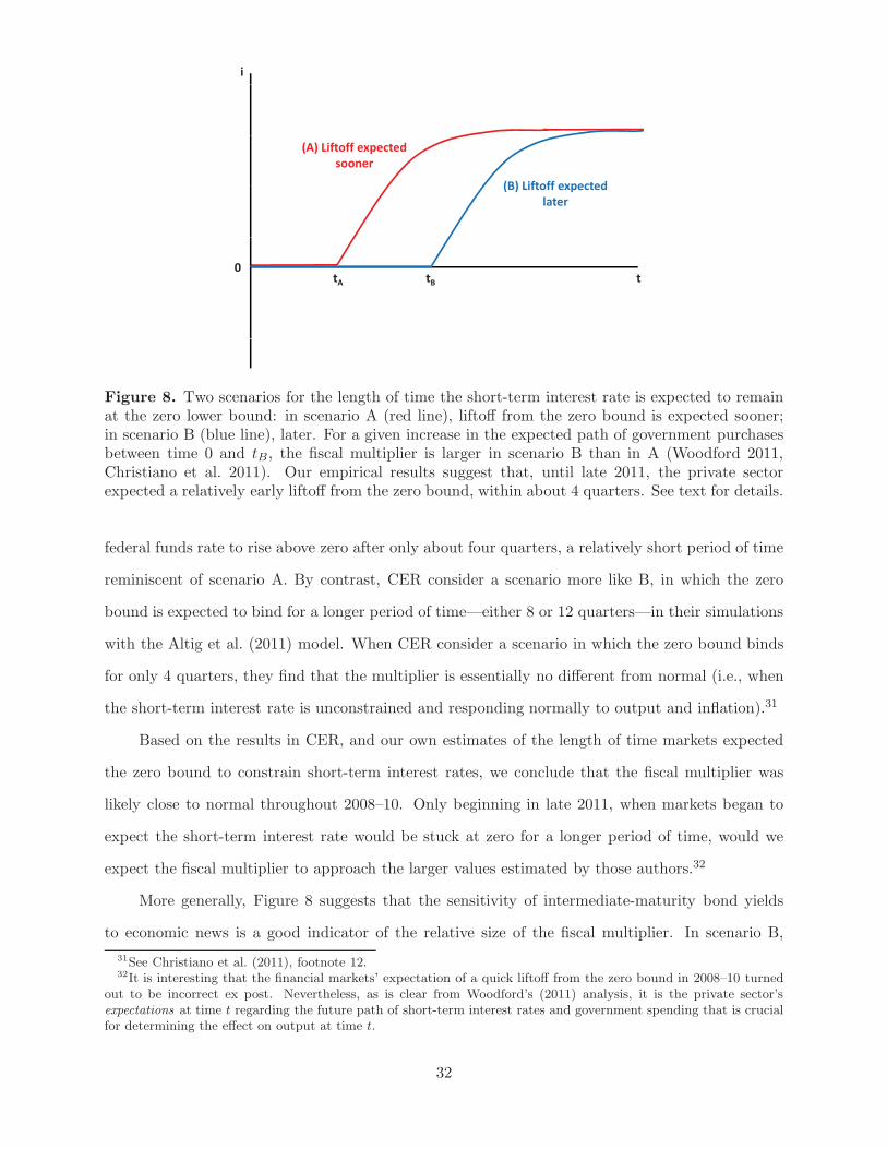
i

(A) Liftoff expectedsooner

(B) Liftoff expected(B) Liftoff expectedlater

t0

tA tB

Figure 8. Two scenarios for the length of time the short-term interest rate is expected to remainat the zero lower bound: in scenario A (red line), liftoff from the zero bound is expected sooner;in scenario B (blue line), later. For a given increase in the expected path of government purchasesbetween time 0 and tB , the fiscal multiplier is larger in scenario B than in A (Woodford 2011,Christiano et al. 2011). Our empirical results suggest that, until late 2011, the private sectorexpected a relatively early liftoff from the zero bound, within about 4 quarters. See text for details.

federal funds rate to rise above zero after only about four quarters, a relatively short period of time

reminiscent of scenario A. By contrast, CER consider a scenario more like B, in which the zero

bound is expected to bind for a longer period of time—either 8 or 12 quarters—in their simulations

with the Altig et al. (2011) model. When CER consider a scenario in which the zero bound binds

for only 4 quarters, they find that the multiplier is essentially no different from normal (i.e., when

the short-term interest rate is unconstrained and responding normally to output and inflation).31

Based on the results in CER, and our own estimates of the length of time markets expected

the zero bound to constrain short-term interest rates, we conclude that the fiscal multiplier was

likely close to normal throughout 2008–10. Only beginning in late 2011, when markets began to

expect the short-term interest rate would be stuck at zero for a longer period of time, would we

expect the fiscal multiplier to approach the larger values estimated by those authors.32

More generally, Figure 8 suggests that the sensitivity of intermediate-maturity bond yields

to economic news is a good indicator of the relative size of the fiscal multiplier. In scenario B,

31See Christiano et al. (2011), footnote 12.32It is interesting that the financial markets’ expectation of a quick liftoff from the zero bound in 2008–10 turned

out to be incorrect ex post. Nevertheless, as is clear from Woodford’s (2011) analysis, it is the private sector’sexpectations at time t regarding the future path of short-term interest rates and government spending that is crucialfor determining the effect on output at time t.

32

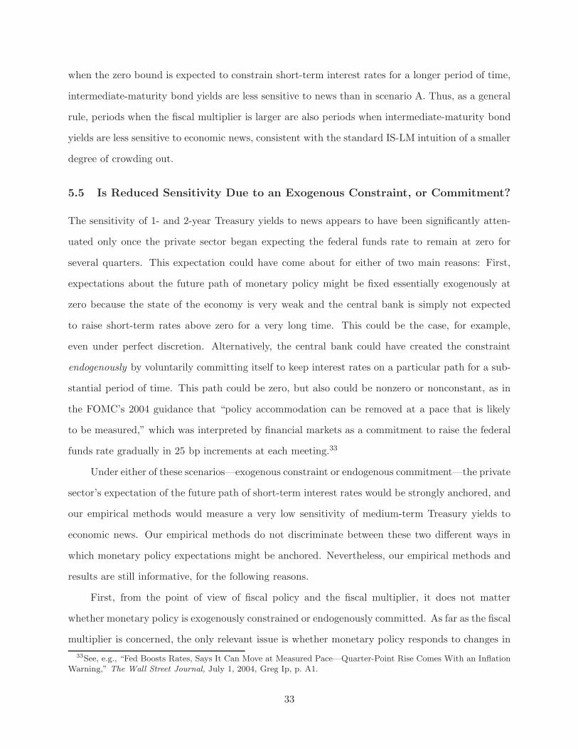
when the zero bound is expected to constrain short-term interest rates for a longer period of time,

intermediate-maturity bond yields are less sensitive to news than in scenario A. Thus, as a general

rule, periods when the fiscal multiplier is larger are also periods when intermediate-maturity bond

yields are less sensitive to economic news, consistent with the standard IS-LM intuition of a smaller

degree of crowding out.

5.5 Is Reduced Sensitivity Due to an Exogenous Constraint, or Commitment?

The sensitivity of 1- and 2-year Treasury yields to news appears to have been significantly atten-

uated only once the private sector began expecting the federal funds rate to remain at zero for

several quarters. This expectation could have come about for either of two main reasons: First,

expectations about the future path of monetary policy might be fixed essentially exogenously at

zero because the state of the economy is very weak and the central bank is simply not expected

to raise short-term rates above zero for a very long time. This could be the case, for example,

even under perfect discretion. Alternatively, the central bank could have created the constraint

endogenously by voluntarily committing itself to keep interest rates on a particular path for a sub-

stantial period of time. This path could be zero, but also could be nonzero or nonconstant, as in

the FOMC’s 2004 guidance that “policy accommodation can be removed at a pace that is likely

to be measured,” which was interpreted by financial markets as a commitment to raise the federal

funds rate gradually in 25 bp increments at each meeting.33

Under either of these scenarios—exogenous constraint or endogenous commitment—the private

sector’s expectation of the future path of short-term interest rates would be strongly anchored, and

our empirical methods would measure a very low sensitivity of medium-term Treasury yields to

economic news. Our empirical methods do not discriminate between these two different ways in

which monetary policy expectations might be anchored. Nevertheless, our empirical methods and

results are still informative, for the following reasons.

First, from the point of view of fiscal policy and the fiscal multiplier, it does not matter

whether monetary policy is exogenously constrained or endogenously committed. As far as the fiscal

multiplier is concerned, the only relevant issue is whether monetary policy responds to changes in

33See, e.g., “Fed Boosts Rates, Says It Can Move at Measured Pace—Quarter-Point Rise Comes With an InflationWarning,” The Wall Street Journal, July 1, 2004, Greg Ip, p. A1.

33

the economic outlook, or not. If the expected path of monetary policy is fixed for the next several

quarters—for whatever reason—the fiscal multiplier will be correspondingly larger, as discussed

in Woodford (2011) and Christiano et al. (2011). Thus, our empirical estimates remain entirely

relevant for the size of the multiplier no matter whether monetary policy is exogenously constrained

at zero, voluntarily committed to zero, or voluntarily committed to some other policy path.

Second, from the point of view of monetary policy, two cases may arise, depending on whether

medium-term Treasury yields are estimated to be sensitive or insensitive to news. In periods

where we estimate Treasury yields are sensitive to news—including the case of partial sensitivity

(0 � δτ < 1)—then we know that monetary policy can still be effective so long as the central

bank can manage monetary policy expectations. This is useful information. Alternatively, in

periods where we estimate Treasury yields are completely insensitive to news (δτ ≈ 0), then the

distinction between an exogenous constraint and voluntary commitment becomes more relevant,

because in principle the central bank might be able to modify its commitment and thereby relax

the constraint. But it is still useful to know whether and when the central bank has come to the

point where intermediate-maturity Treasury yields are no longer sensitive to news.

Finally, we emphasize that the distinction between an exogenous constraint on the central

bank and an endogenous commitment to a policy path is not so sharp in practice. For example,

it is precisely because of the zero lower bound that the FOMC issued its “mid-2013”, “late 2014”,

and “mid-2015” forward guidance.34 Even if this forward guidance was voluntary, it was clearly

motivated by the (exogenous) presence of the zero lower bound. Thus, one can make a strong

argument that, whatever the direct reason for the lower sensitivity we estimate in 2011–12, that

reduced sensitivity is ultimately due to the presence of the zero lower bound constraint.

5.6 Other Explanations for Time-Varying Sensitivity

The sensitivity of Treasury yields to news could also vary for reasons other than the zero bound

constraint. For example, it is well known that interest rate volatility increases with the level of

rates (e.g., Chan, Karolyi, Longstaff, and Sanders 1992); thus, part of our estimated decline in

Treasury yield sensitivity since 2009 could simply reflect the decline in Treasury yields over that

34On September 13, 2012, the FOMC announced that it expected to keep the funds rate near zero through at least“mid-2015”.

34

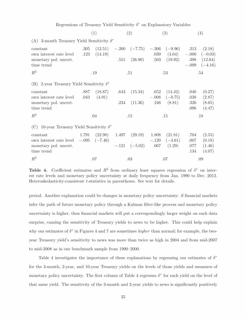
Regressions of Treasury Yield Sensitivity δτ on Explanatory Variables

(1) (2) (3) (4)

(A) 3-month Treasury Yield Sensitivity δτ

constant .305 (12.51) −.260 (−7.75) −.306 (−9.96) .313 (2.18)own interest rate level .123 (14.19) .039 (4.64) −.000 (−0.03)monetary pol. uncert. .551 (26.90) .503 (19.92) .398 (12.64)time trend −.099 (−4.16)

R2 .19 .51 .53 .54

(B) 2-year Treasury Yield Sensitivity δτ

constant .887 (18.87) .643 (15.34) .652 (14.42) .040 (0.27)own interest rate level .043 (4.91) −.008 (−0.75) .038 (2.87)monetary pol. uncert. .234 (11.36) 246 (8.81) .326 (8.65)time trend .096 (4.47)

R2 .04 .15 .15 .18

(C) 10-year Treasury Yield Sensitivity δτ

constant 1.791 (22.98) 1.497 (29.19) 1.808 (21.81) .704 (2.55)own interest rate level −.095 (−7.46) −.120 (−4.61) .007 (0.18)monetary pol. uncert. −.121 (−5.02) .067 (1.29) .077 (1.46)time trend .134 (4.07)

R2 .07 .03 .07 .09

Table 4. Coefficient estimates and R2 from ordinary least squares regression of δτ on inter-est rate levels and monetary policy uncertainty at daily frequency from Jan. 1990 to Dec. 2012.Heteroskedasticity-consistent t-statistics in parentheses. See text for details.

period. Another explanation could be changes in monetary policy uncertainty: if financial markets

infer the path of future monetary policy through a Kalman filter-like process and monetary policy

uncertainty is higher, then financial markets will put a correspondingly larger weight on each data

surprise, causing the sensitivity of Treasury yields to news to be higher. This could help explain

why our estimates of δτ in Figures 4 and 7 are sometimes higher than normal; for example, the two-

year Treasury yield’s sensitivity to news was more than twice as high in 2004 and from mid-2007

to mid-2008 as in our benchmark sample from 1990–2000.

Table 4 investigates the importance of these explanations by regressing our estimates of δτ

for the 3-month, 2-year, and 10-year Treasury yields on the levels of those yields and measures of

monetary policy uncertainty. The first column of Table 4 regresses δτ for each yield on the level of

that same yield. The sensitivity of the 3-month and 2-year yields to news is significantly positively

35

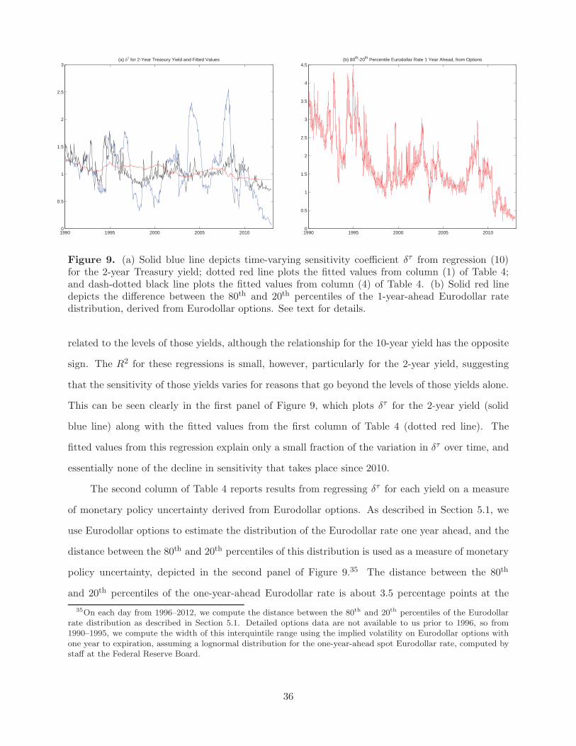
1990 1995 2000 2005 20100

0.5

1

1.5

2

2.5

3(a) for 2-Year Treasury Yield and Fitted Values

1990 1995 2000 2005 20100

0.5

1

1.5

2

2.5

3

3.5

4

4.5(b) 80th-20th Percentile Eurodollar Rate 1 Year Ahead, from Options

Figure 9. (a) Solid blue line depicts time-varying sensitivity coefficient δτ from regression (10)for the 2-year Treasury yield; dotted red line plots the fitted values from column (1) of Table 4;and dash-dotted black line plots the fitted values from column (4) of Table 4. (b) Solid red linedepicts the difference between the 80th and 20th percentiles of the 1-year-ahead Eurodollar ratedistribution, derived from Eurodollar options. See text for details.

related to the levels of those yields, although the relationship for the 10-year yield has the opposite

sign. The R2 for these regressions is small, however, particularly for the 2-year yield, suggesting

that the sensitivity of those yields varies for reasons that go beyond the levels of those yields alone.

This can be seen clearly in the first panel of Figure 9, which plots δτ for the 2-year yield (solid

blue line) along with the fitted values from the first column of Table 4 (dotted red line). The

fitted values from this regression explain only a small fraction of the variation in δτ over time, and

essentially none of the decline in sensitivity that takes place since 2010.

The second column of Table 4 reports results from regressing δτ for each yield on a measure

of monetary policy uncertainty derived from Eurodollar options. As described in Section 5.1, we

use Eurodollar options to estimate the distribution of the Eurodollar rate one year ahead, and the

distance between the 80th and 20th percentiles of this distribution is used as a measure of monetary

policy uncertainty, depicted in the second panel of Figure 9.35 The distance between the 80th

and 20th percentiles of the one-year-ahead Eurodollar rate is about 3.5 percentage points at the

35On each day from 1996–2012, we compute the distance between the 80th and 20th percentiles of the Eurodollarrate distribution as described in Section 5.1. Detailed options data are not available to us prior to 1996, so from1990–1995, we compute the width of this interquintile range using the implied volatility on Eurodollar options withone year to expiration, assuming a lognormal distribution for the one-year-ahead spot Eurodollar rate, computed bystaff at the Federal Reserve Board.

36

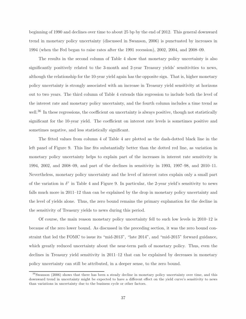
beginning of 1990 and declines over time to about 25 bp by the end of 2012. This general downward

trend in monetary policy uncertainty (discussed in Swanson, 2006) is punctuated by increases in

1994 (when the Fed began to raise rates after the 1991 recession), 2002, 2004, and 2008–09.

The results in the second column of Table 4 show that monetary policy uncertainty is also

significantly positively related to the 3-month and 2-year Treasury yields’ sensitivities to news,

although the relationship for the 10-year yield again has the opposite sign. That is, higher monetary

policy uncertainty is strongly associated with an increase in Treasury yield sensitivity at horizons

out to two years. The third column of Table 4 extends this regression to include both the level of

the interest rate and monetary policy uncertainty, and the fourth column includes a time trend as

well.36 In these regressions, the coefficient on uncertainty is always positive, though not statistically

significant for the 10-year yield. The coefficient on interest rate levels is sometimes positive and

sometimes negative, and less statistically significant.

The fitted values from column 4 of Table 4 are plotted as the dash-dotted black line in the

left panel of Figure 9. This line fits substantially better than the dotted red line, as variation in

monetary policy uncertainty helps to explain part of the increases in interest rate sensitivity in

1994, 2002, and 2008–09, and part of the declines in sensitivity in 1993, 1997–98, and 2010–11.

Nevertheless, monetary policy uncertainty and the level of interest rates explain only a small part

of the variation in δτ in Table 4 and Figure 9. In particular, the 2-year yield’s sensitivity to news

falls much more in 2011–12 than can be explained by the drop in monetary policy uncertainty and

the level of yields alone. Thus, the zero bound remains the primary explanation for the decline in

the sensitivity of Treasury yields to news during this period.

Of course, the main reason monetary policy uncertainty fell to such low levels in 2010–12 is

because of the zero lower bound. As discussed in the preceding section, it was the zero bound con-

straint that led the FOMC to issue its “mid-2013”, “late 2014”, and “mid-2015” forward guidance,

which greatly reduced uncertainty about the near-term path of monetary policy. Thus, even the

declines in Treasury yield sensitivity in 2011–12 that can be explained by decreases in monetary

policy uncertainty can still be attributed, in a deeper sense, to the zero bound.

36Swanson (2006) shows that there has been a steady decline in monetary policy uncertainty over time, and thisdownward trend in uncertainty might be expected to have a different effect on the yield curve’s sensitivity to newsthan variations in uncertainty due to the business cycle or other factors.

37

5.7 Post-2007 Distribution of Macroeconomic Data Release Surprises

In our main empirical regressions (9) and (10), the surprise component of each data release in Xt

can be regarded as strictly exogenous, under the assumption that our survey expectations data

incorporate all relevant information as of the day before the release. (Under this assumption, the

surprise component of each data release is independent of all past and future values of the interest

rate changes on the left-hand side of these regressions.) To the extent that regressions (9) and

(10) are correctly specified, strict exogeneity then implies that the empirical distribution of the

macroeconomic surprise data Xt is irrelevant for our estimates of the relative response coefficients

β or time-varying sensitivity coefficients δ.

Nevertheless, one might be concerned that regression specifications (9) and (10) are simplifi-

cations that assume a linear structure with respect to Xt. As a result, it would be reassuring if the

distribution of data surprises Xt in 2008–12 was not dramatically different from our benchmark

sample 1990–2000, or the pre-crisis sample 1990–2007.

In fact, the distribution of these macro data surprises is similar across these samples. This

can be seen in Figure 10, which plots the surprise component of nonfarm payrolls and core CPI

announcements over the 1990–2007 and 2008–12 periods. Results for other macroeconomic data

releases and the 1990–2000 period are similar. This finding might seem puzzling at first given the

severity of the 2007–09 recession, but one should bear in mind that financial markets were quick

to realize the severity of the downturn, so financial market expectations of the data fell about in

line with the decline in the data itself. As a result, the surprises in the data releases, relative to

the one-day-ahead expectations, do not look very different from earlier periods.

6 Conclusions

In this paper, we have developed a novel method to measure whether and to what extent interest

rates of any maturity are affected by the presence of the zero lower bound. Our method provides

both a quantitative measure of the severity of the zero bound constraint on each yield and a

statistical test for the periods during which that yield was affected.

We find that interest rates with a year or more to maturity were surprisingly responsive to

38

-400 -300 -200 -100 0 100 200 300 4000

5

10

15

20

25

30

35

40

45

50

55(a) Nonfarm Payrolls Surprises, 1990-2007

-400 -300 -200 -100 0 100 200 300 4000

2

4

6

8

10

12

14

16

(b) Nonfarm Payrolls Surprises, 2008-2012

-0.4 -0.3 -0.2 -0.1 0 0.1 0.2 0.3 0.40

10

20

30

40

50

60

70

80

90(c) Core CPI Surprises, 1990-2007

-0.4 -0.3 -0.2 -0.1 0 0.1 0.2 0.3 0.40

5

10

15

20

(d) Core CPI Surprises, 2008-2012

Figure 10. Top panels depict empirical distribution of the surprise component of nonfarm payrollsannouncements from (a) 1990–2007 and (b) 2008–12, rounded to the nearest 50 thousand workers.Bottom panels depict the distribution of core CPI surprises from (c) 1990–2007 and (d) 2008–12,rounded to the nearest 0.1 percent. The surprise distributions of these and other macroeconomicdata releases are relatively similar pre- and post-crisis. See text for details.

news throughout 2008–10. Only beginning in late 2011—around the time of the FOMC’s “mid-

2013” forward guidance—do we see the sensitivity of intermediate-maturity Treasury yields fall

closer to zero. There appear to be two main explanations for this finding: First, up until late 2011,

financial markets consistently expected the federal funds rate to lift off from zero within about

four quarters. Second, the FOMC’s forward guidance and large-scale asset purchases—and private-

sector expectations of Federal Reserve policies along these lines—continued to move medium- and

longer-term interest rates even when short-term rates were stuck at zero.

Our results have important implications for both monetary and fiscal policy. For monetary

39

policy, our findings imply that policymakers had substantial room to affect medium- and longer-

term interest rates until at least late 2011, despite the federal funds rate being at the zero lower

bound. Indeed, on several occasions, the FOMC appears to have directly affected those longer-term

yields by managing expectations of future monetary policy and conducting large-scale purchases of

longer-term bonds.

For fiscal policy, taking the results in Christiano et al. (2011) as given, our findings suggest that

the fiscal multiplier was probably close to normal throughout 2008–10, because financial markets

at that time expected the zero bound constraint to last only about four quarters or less. Only

beginning in late 2011, when the sensitivity of two-year Treasury yields to news was reduced—and

the expected time until the first federal funds rate increase was lengthened to seven quarters or

more—would our results suggest that the fiscal multiplier approached the larger values estimated

by Christiano et al. (2012) and other authors.

More generally, the methods we have developed in the present paper can be extended beyond

the United States and applied to any economy for which financial markets are sufficiently well

developed. In particular, it would be very interesting to see our methods applied to other economies

that have faced the zero lower bound in recent years, such as Japan, the U.K., Canada, Sweden,

and the Euro area.

40

References

Altig, David, Lawrence J. Christiano, Martin Eichenbaum, and Jesper Linde, “Firm-Specific Cap-ital, Nominal Rigidities, and the Business Cycle,” Review of Economic Dynamics 14, 2011,225–247.

Andersen, Torben G., Tim Bollerslev, Francis X. Diebold, and Clara Vega, “Micro Effects of MacroAnnouncements: Real-Time Price Discovery in Foreign Exchange,” American Economic Review93(1), 2003, 38–62.

Bernanke, Ben S., and Vincent R. Reinhart, “Conducting Monetary Policy at Very Low Short-TermInterest Rates,” American Economic Review, Papers and Proceedings 94(2), 2004, 85–90.

Bernanke, Ben S., Vincent R. Reinhart, and Brian P. Sack, “Monetary Policy Alternatives at theZero Bound: An Empirical Assessment,” Brookings Papers on Economic Activity, Fall 2004,1–78.

Blue Chip, Blue Chip Financial Forecasts, New York, NY: Aspen Publishers, various issues from2008–2012.

Campbell, Jeffrey, Charles Evans, Jonas Fisher, and Alejandro Justiniano, “Macroeconomic Effectsof FOMC Forward Guidance,” Brookings Papers on Economic Activity, Spring 2012, 1–54.

Chan, K.C., G. Andrew Karolyi, Francis Longstaff, and Anthony Sanders, “An Empirical Com-parison of Alternative Models of the Short-Term Interest Rate,” Journal of Finance 47, 1992,1209–1227.

Christiano, Lawrence, Martin Eichenbaum, and Sergio Rebelo, “When is the Government SpendingMultiplier Large?” Journal of Political Economy 119, 2011, 78–121.

Clarida, Richard, Jordi Galı, and Mark Gertler, “The Science of Monetary Policy,” Journal ofEconomic Literature 37, 1999, 1661–1707.

Debortoli, Davide and Ricardo Nunes, “Fiscal Policy under Loose Commitment,” Journal of Eco-nomic Theory 145(3), 2010, 1005–1032.

DeLong, J. Bradford and Lawrence Summers, “Fiscal Policy in a Depressed Economy,” BrookingsPapers on Economic Activity, Spring 2012, 233–274.

Eggertsson, Gauti B., “What Fiscal Policy is Effective at Zero Interest Rates?” Federal ReserveBank of New York Staff Report 402, 2009.

Eggertsson, Gauti B., and Paul Krugman, “Debt, Deleveraging, and the Liquidity Trap: A Fisher-Minsky-Koo Approach,” Quarterly Journal of Economics 2012, 1469–1513.

Eggertsson, Gauti B., and Michael Woodford, “The Zero Interest-Rate Bound and Optimal Mon-etary Policy,” Brookings Papers on Economic Activity, Spring 2003, 139–211.

Erceg, Christopher J., and Jesper Linde, “Is There a Fiscal Free Lunch in a Liquidity Trap?” FederalReserve Board International Finance Discussion Paper 2010–1003, 2010.

Gagnon, Joseph, Matthew Raskin, Julie Remache, and Brian Sack,“The Financial Market Effects ofthe Federal Reserves Large-Scale Asset Purchases.” International Journal of Central Banking,7(1), March 2011, 3–43.

Gurkaynak, Refet, Andrew Levin, and Eric Swanson, “Does Inflation Targeting Anchor Long-RunInflation Expectations? Evidence from the U.S., UK, and Sweden,” Journal of the EuropeanEconomic Association, 8(6), 2010, 1208–1242.

41

Gurkaynak, Refet, Brian Sack, and Eric Swanson, “The Sensitivity of Long-Term Interest Rates toEconomic News: Evidence and Implication for Macroeconomic Models.” American EconomicReview, 95(1), 2005a, 426–436.

Gurkaynak, Refet, Brian Sack, and Eric Swanson, “Do Actions Speak Louder than Words? TheResponse of Asset Prices to Monetary Policy Actions and Statements,” International Journalof Central Banking 1(1), 2005b, 55–93.

Gurkaynak, Refet, Brian Sack, and Eric Swanson, “Market-Based Measures of Monetary PolicyExpectations.” Journal of Business and Economic Statistics 25(2), 2007, 201–212.

Gurkaynak, Refet, Brian Sack, and Jonathan Wright, “The U.S. Treasury Yield Curve: 1961 to thePresent,” Journal of Monetary Economics 54, 2007, 2291–2304.

Hamilton, James, and Jing (Cynthia) Wu, “The Effectiveness of Alternative Monetary Policy Toolsin a Zero Lower Bound Environment,” Journal of Money, Credit, and Banking 44(S1), 2012,3–46.

Kohn, Donald, and Brian Sack, “Central Bank Talk: Does It Matter and Why?” inMacroeconomics,Monetary Policy, and Financial Stability, Ottawa: Bank of Canada, 2004.

Krishnamurthy, Arvind, and Annette Vissing-Jorgensen, “The Effects of Quantitative Easing onInterest Rates: Channels and Implications for Policy,” Brookings Papers on Economic Activity,Fall 2011, 215–265.

Krishnamurthy, Arvind, and Annette Vissing-Jorgensen, “The Aggregate Demand for TreasuryDebt,” Journal of Political Economy 120, 2012, 233–267.

Kuttner, Kenneth N., “Monetary policy surprises and interest rates: Evidence from the Fed fundsfutures market.” Journal of Monetary Economics 47(3), 2001, 523–544.

Kydland, Finn, and Edward C. Prescott, “Rules Rather than Discretion: The Inconsistency ofOptimal Plans,” Journal of Political Economy, 85(3), 1977, 473–492.

Modigliani, Franco, and Richard Sutch, “Innovations in Interest Rate Policy,” American EconomicReview, 56(1), 1966, 178–197.

Reifschneider, David, and John C. Williams, “Three Lessons for Monetary Policy in a Low InflationEra,” Journal of Money, Credit and Banking 32(4), 2000, 936–966.

Sack, Brian, and Volker Wieland, “Interest-Rate Smoothing and Optimal Monetary Policy: A Re-view of Recent Empirical Evidence,” Journal of Economics and Business 52, 2000, 205–228.

Schaumburg, Ernst, and Andrea Tambalotti, “An Investigation of the Gains from Commitment inMonetary Policy,” Journal of Monetary Economics 54(2), 2007, 302–324.

Sims, Christopher A., and Tao Zha, “Error Bands for Impulse Responses,” Econometrica 67(5),1999, 1113–1155.

Swanson, Eric T., “Have Increases in Federal Reserve Transparency Improved Private Sector In-terest Rate Forecasts?” Journal of Money, Credit, and Banking 38, 2006, 791–819.

Swanson, Eric T., “Let’s Twist Again: A High-Frequency Event-Study Analysis of Operation Twistand Its Implications for QE2,” Brookings Papers on Economic Activity, Spring 2011, 151–188.

Taylor, John, “Discretion Versus Policy Rules in Practice,” Carnegie-Rochester Conference Serieson Public Policy, 39, 1993, 195–214.

Tobin, James, “Liquidity Preference as Behavior Toward Risk,” Review of Economic Studies, 25,1958, 124–131.

42

Vayanos, Dimitri, and Jean-Luc Vila, “A Preferred-Habitat Model of the Term Structure of InterestRates,” NBER Working Paper 15487, 2009.

Woodford, Michael, Interest and Prices: Foundations of a Theory of Monetary Policy, Princeton:Princeton University Press, 2003.

Woodford, Michael, “Simple Analytics of the Government Expenditure Multiplier,” American Eco-nomic Journal: Macroeconomics 3, 2011, 1–35.

43