measuring the complexity of simulated engineering … golnaz is working with the epistemic games...
TRANSCRIPT

Paper ID #11437
Measuring the Complexity of Simulated Engineering Design Problems
Ms. Golnaz Arastoopour, University of Wisconsin, Madison
Before becoming interested in education, Golnaz studied Mechanical Engineering at the University of Illi-nois at Urbana-Champaign with a minor in Spanish. While earning her Bachelor’s degree in engineering,she worked as a computer science instructor at Campus Middle School for Girls in Urbana, IL. Along witha team of undergraduates, she headlined a project to develop a unique computer science curriculum formiddle school students. She then earned her M.A. in mathematics education at Columbia University. Af-terwards, she taught in the Chicago Public School system at Orr Academy High School (an AUSL school)for two years. Currently, Golnaz is working with the Epistemic Games Research Group at the Universityof Wisconsin-Madison where she has led the efforts on engineering virtual internship simulations for highschool and first year undergraduate students. Golnaz’s current research is focused on how games and sim-ulations increase student engagement in STEM fields, how players learn engineering design in real-worldand virtual professional environments, and how to assess engineering design thinking.
Prof. David Williamson ShafferDr. Naomi C. Chesler, University of Wisconsin, Madison
Naomi C. Chesler is Professor and Vice Chair of Biomedical Engineering with an affiliate appointmentin Educational Psychology. Her research interests include vascular biomechanics, hemodynamics andcardiac function as well as the factors that motivate students to pursue and persist in engineering careers,with a focus on women and under-represented minorities.
Wesley Collier, University of Wisconsin-Madison
Wesley Collier is a graduate student in learning sciences in the Epistemic Games research group at theUniversity of Wisconsin-Madison working on the Epistemic Network Analysis tool. He is interested inhow games and simulations can be assessed using discourse analysis.
Jeff Linderoth, University of Wisconsin-Madison
c©American Society for Engineering Education, 2015
Page 26.1140.1
Measuring the Complexity of Simulated Engineering Design
Problems
Abstract
The ability of tomorrow’s engineering professionals to solve complex real-world problems is
dependent on their education and training. We posit that engineering education and training in
design would be improved by presenting students with design challenges with increasing levels
of complexity as they advance in engineering curricula. In order to construct design challenges
with increasing levels of complexity, a framework for assessing the complexity of engineering
design problems must be developed. As a first step toward this goal, we consider the complexity
of simulated design problems, which have been previously developed as part of virtual
engineering internships and which have the advantages of being well-defined and solvable. In
this paper, we present a parameterized, mathematical model to quantify engineering design
problem complexity. In particular, we present three functions that model the process by which a
student moves from information provided and assumptions to predicting design performance and
then to a final design choice. These functions are �̂�, students’ predictions of device
performance, 𝑽, how students value performance criteria, and 𝑷 how students develop
preferences for specific designs. Finally, based on this framework for quantifying simulated
design problem complexity, we present a metric of complexity, tractability 𝑻, supported by data
from real student work on a simulated engineering design problem.
Theory
Engineering Design Education
Design is a critical part of the engineering profession [1], [2]. As a result, design is a central
focus of engineering education in terms of teaching, learning, and assessment [3], [4]. In a recent
study, Sheppard and others [5] interviewed faculty and students about the field of engineering
and concluded that design is the most critical component of engineering education. One faculty
member asserted that “guiding students to learn ‘design thinking’ and the design process, so
central to professional practice, is the responsibility of engineering education” (p. 98).
Two decades ago, ABET, the accreditation board for engineering programs, developed criteria
that included opportunities for design learning. ABET [6] defined engineering design as the
“process of devising a system, component, or process to meet desired needs. It is a decision-
making process (often iterative), in which the basic sciences, mathematics, and the engineering
sciences are applied to convert resources optimally to meet these stated needs” (p. 4). The
criteria require that students engage in a major design project.
In response to these requirements, universities developed senior-level capstone courses. Either in
teams or as individuals, students design a product or a process in these courses. They present
their work orally or in a final written report, which the instructor evaluates. The basic purpose of
these courses is for students to engage in design activities that are based on real-world
engineering practice. Harrisberger and others [7] have categorized real-world experiential
learning into two categories: simulated and authentic. Simulations are contrived learning
conditions that are carefully designed and controlled by instructors. Authentic learning
Page 26.1140.2
conditions have students solve real problems in real environments, such as an internship within a
company. The majority of capstone courses occur over one or two semesters during the final year
of the undergraduate program [8].
In contrast, cornerstone courses are design courses for first-year undergraduate students. Many
of these courses were developed to reduce attrition and increase persistence in engineering by
engaging students in design work early in the curriculum [9], [10]. Dym [11] argues that
although freshmen students do not have the engineering technical knowledge to engage in design
at the level of professional engineers, freshmen are still able to “take chances at putting together
components, matching them in a systems-like approach, recognizing performance characteristics
and linking components accordingly” (p. 1). In the cornerstone-capstone model, students engage
in a design course in the first and final year of the undergraduate program with little design
experience in between.
In recent years, as conceptions of engineering design thinking have broadened and become more
complex [3], the capstone-cornerstone curriculum model has been shown to be inadequate [12].
Consequently, there are now programs that are taking an integrated design approach where
design experiences are incorporated throughout the curriculum [13], [14]. This gives students a
more holistic engineering design experience, allows time for design thinking to develop, and
exposes students to various design scenarios. For example, the biomedical engineering
department at the University of Wisconsin-Madison requires that students enroll in six semesters
of design courses. Students work in teams to solve a real-world problem posed by a client, which
could be a faculty member, clinician, industry partner, and or a person in the community with a
biomedical challenge. Teams are advised by faculty members and in some courses, novice
students are mentored by senior students. Several of the students’ design work has resulted in
winning national competitions, journal publications, and numerous patents for the developed
products [15], [16].
Following the University of Wisconsin-Madison example, there is a movement towards greater
integration of design throughout undergraduate engineering curricula [4]. If integrated design is
an effective and desirable method for exposing engineering students to design learning, then
design problem complexity must be adjusted for students at various levels, from the novice first
year to the more experienced senior student.
Decision Based Engineering Design
Two obvious aspects of design problem complexity are the number of performance criteria the
client has for the final device and the number of design options that the student must consider.
The more functions the device must perform and the higher the standards of performance, the
more challenging it is to solve; the more open-ended the design problem, the more daunting the
task for the student engineer. Independent of the number of input choices and output parameters,
a design problem is more difficult to solve if the student has less information about the problem
and less knowledge about how performance criteria depend on design choices. The process of
selecting a final design based on information, knowledge or assumptions, input choices and
output parameters is one aspect of decision-making. In considering the complexity of solving
design problems, here we focus on this decision-making aspect.
Page 26.1140.3

In the literature, engineering design decision-making has been parameterized and represented
mathematically. For example, Hazelrigg [17] argues for a mathematics of design based on
decision theory [18], which is now identified as decision-based engineering design. Hazelrigg
constructed a set of axioms for designing and formulated two theorems that could be applied to
statistical models that account for uncertainty, risk, information, preferences, and external
factors. For example, the expected utility theorem states that given a pair of designs, each with a
range of possible outcomes and associated probabilities of occurrence, the preferred choice is the
alternative that has the highest expected utility. Relatedly, Tian and others (1994) have shown
that uncertainty plays a large role in engineering design decision making. They argue that
uncertainty occurs in engineering design because in many cases, performance parameters can
only be estimated, particularly manufacturing costs. This uncertainty affects the designer’s
perception of the desirability of choices and a risk analysis may come into play. Building on this
work, Thurston [19] developed a model that considers tradeoff decisions under uncertainty and
models how the designer may choose to optimize several performance parameters at a time.
Radford and Gero [20] describe design as a goal-seeking activity and developed a model that
focuses on optimization of design goals. Finally, others have explored pairwise analyses when
making design decisions [21], [22]. To date, these models have not been applied to student
engineers in a learning environment or studied within a well-defined and solvable design space
such as a simulated engineering design problem.
Simulated Engineering Design
In order to develop a mathematical model to quantify engineering design problem complexity for
integrating design throughout undergraduate engineering curricula, we considered how students
solve simulated engineering design problems. An advantage of this approach is that the numbers
of input choices and performance parameters, as well as the information provided, are fixed such
that student decision-making is the critical factor in design problem complexity.
The simulated design problems considered in this study are within virtual internships that our
group has previously developed for first-year introduction to engineering design courses:
Nephrotex and RescuShell. As has been described in detail elsewhere [23], [24], students in
Nephrotex role-play as interns to design a filtration membrane for a hemodialysis machine and
students in RescuShell design an exoskeleton to assist rescue workers. In each internship
program, students log on to a web interface that simulates a company work portal where they
receive tasks from a supervisor. Individually they conduct background research, summarize
customer requests and technical constraints, and then, in teams, design and test several devices
before deciding on a final prototype. When deciding on a final prototype, students consider
conflicting stakeholder requests and choose a design that best meets all of the stated thresholds.
For example, the clinical engineer is concerned about blood cell reactivity and flux, and the
manufacturing engineer values reliability and cost. At the end of the course, students present
their work to their colleagues and instructor.
We use the simulated design problems in Nephrotex and RescuShell as representations of real
design problems and examine how to measure design problem complexity by focusing on
student decision-making. Specifically in this study, we (1) describe and define the design
parameters and variables related to decision making in Nephrotex, (2) mathematically describe
the decision making process in Nephrotex, (3) define a novel metric for quantifying the difficulty
Page 26.1140.4
of solving these simulated design problems, and (4) compare the difficulties or complexities of
the simulated engineering design problems within Nephrotex and RescuShell supported by
student data.
Framework for Assessing Simulated Design Problem Complexity
Elements in the Design Space
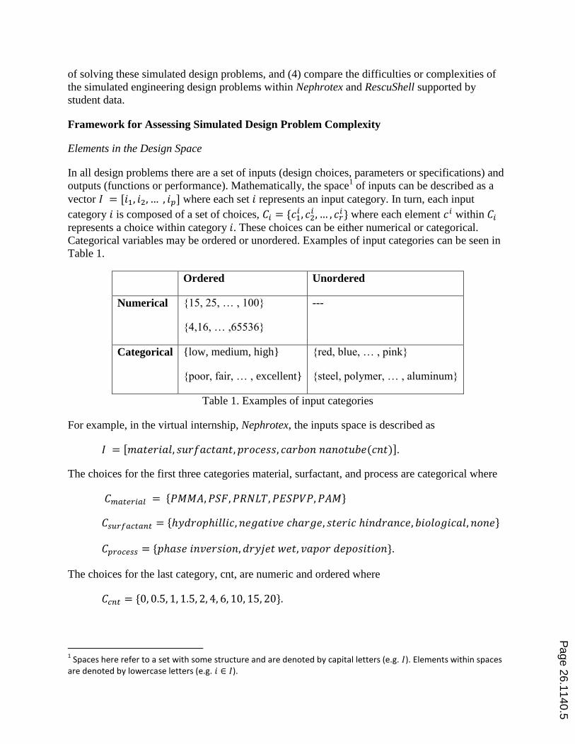
In all design problems there are a set of inputs (design choices, parameters or specifications) and
outputs (functions or performance). Mathematically, the space1 of inputs can be described as a
vector 𝐼 = [𝑖1, 𝑖2, … , 𝑖𝑝] where each set 𝑖 represents an input category. In turn, each input
category 𝑖 is composed of a set of choices, 𝐶𝑖 = {𝑐1𝑖 , 𝑐2
𝑖 , … , 𝑐𝑟𝑖 } where each element 𝑐𝑖 within 𝐶𝑖
represents a choice within category 𝑖. These choices can be either numerical or categorical.
Categorical variables may be ordered or unordered. Examples of input categories can be seen in
Table 1.
Ordered Unordered
Numerical {15, 25, … , 100}
{4,16, … ,65536}
---
Categorical {low, medium, high}
{poor, fair, … , excellent}
{red, blue, … , pink}
{steel, polymer, … , aluminum}
Table 1. Examples of input categories
For example, in the virtual internship, Nephrotex, the inputs space is described as
𝐼 = [𝑚𝑎𝑡𝑒𝑟𝑖𝑎𝑙, 𝑠𝑢𝑟𝑓𝑎𝑐𝑡𝑎𝑛𝑡, 𝑝𝑟𝑜𝑐𝑒𝑠𝑠, 𝑐𝑎𝑟𝑏𝑜𝑛 𝑛𝑎𝑛𝑜𝑡𝑢𝑏𝑒(𝑐𝑛𝑡)].
The choices for the first three categories material, surfactant, and process are categorical where
𝐶𝑚𝑎𝑡𝑒𝑟𝑖𝑎𝑙 = {𝑃𝑀𝑀𝐴, 𝑃𝑆𝐹, 𝑃𝑅𝑁𝐿𝑇, 𝑃𝐸𝑆𝑃𝑉𝑃, 𝑃𝐴𝑀}
𝐶𝑠𝑢𝑟𝑓𝑎𝑐𝑡𝑎𝑛𝑡 = {ℎ𝑦𝑑𝑟𝑜𝑝ℎ𝑖𝑙𝑙𝑖𝑐, 𝑛𝑒𝑔𝑎𝑡𝑖𝑣𝑒 𝑐ℎ𝑎𝑟𝑔𝑒, 𝑠𝑡𝑒𝑟𝑖𝑐 ℎ𝑖𝑛𝑑𝑟𝑎𝑛𝑐𝑒, 𝑏𝑖𝑜𝑙𝑜𝑔𝑖𝑐𝑎𝑙, 𝑛𝑜𝑛𝑒}
𝐶𝑝𝑟𝑜𝑐𝑒𝑠𝑠 = {𝑝ℎ𝑎𝑠𝑒 𝑖𝑛𝑣𝑒𝑟𝑠𝑖𝑜𝑛, 𝑑𝑟𝑦𝑗𝑒𝑡 𝑤𝑒𝑡, 𝑣𝑎𝑝𝑜𝑟 𝑑𝑒𝑝𝑜𝑠𝑖𝑡𝑖𝑜𝑛}.
The choices for the last category, cnt, are numeric and ordered where
𝐶𝑐𝑛𝑡 = {0, 0.5, 1, 1.5, 2, 4, 6, 10, 15, 20}.
1 Spaces here refer to a set with some structure and are denoted by capital letters (e.g. 𝐼). Elements within spaces
are denoted by lowercase letters (e.g. 𝑖 ∈ 𝐼).
Page 26.1140.5

A potential solution for a design problem, i.e., a set of design choices within the design space,
can be described as a vector 𝑥 = [𝑥𝑖1, 𝑥𝑖2
, … , 𝑥𝑖𝑝] for which there is one choice for every input
category, 𝑖. All solution vectors, 𝑥, are within the solution space 𝑋, that is 𝑥 ∈ 𝑋 where 𝑋 =×𝑖∈𝐼 𝐶𝑖, the cross product of all the possible choices in all the categories. That is, 𝑋 is a space
defined by all possible combinations of choices for each input category. There are 4 input
categories in Nephrotex, so 𝑥 is always a vector with 4 elements,
[𝑥𝑚𝑎𝑡𝑒𝑟𝑖𝑎𝑙, 𝑥𝑠𝑢𝑟𝑓𝑎𝑐𝑡𝑎𝑛𝑡, 𝑥𝑝𝑟𝑜𝑐𝑒𝑠𝑠, 𝑥𝑐𝑛𝑡]. One example of a solution (or possible device design) in
Nephrotex is
𝑥 = [𝑃𝐴𝑀, 𝐻𝑦𝑑𝑟𝑜𝑝ℎ𝑖𝑙𝑖𝑐, 𝑃ℎ𝑎𝑠𝑒 𝐼𝑛𝑣𝑒𝑟𝑠𝑖𝑜𝑛, 2%].
In addition, there is a larger input space, �̇�, that is defined as the space of all theoretical input
combinations that may not be available to the designer, potentially because of technical or
financial limitations. Thus, the space 𝑋 is more clearly defined as the set of all input
combinations that are available to the designer where 𝑋 ⊂ �̇�.
In design problems, there is also an output space, where 𝑂 = [𝑜1, 𝑜2, … , 𝑜𝑛], in which each
element of 𝑜 is an aspect of design function or performance. The performance of every solution
to the design problem, which we call 𝑦, must reside within the output space, that is 𝑦 ∈ 𝑂. In
general, the performance is a 𝑛 dimensional vector [𝑦1, 𝑦2, … , 𝑦𝑛] for which there is one real
number value2 for every output category. In Nephrotex, there are five aspects of performance for
which the student is designing, so the vector 𝑂 has five components:
𝑂 = [𝑚𝑎𝑟𝑘𝑒𝑡𝑎𝑏𝑖𝑙𝑖𝑡𝑦, 𝑐𝑜𝑠𝑡, 𝑟𝑒𝑙𝑖𝑎𝑏𝑖𝑙𝑖𝑡𝑦, 𝑓𝑙𝑢𝑥, 𝑏𝑙𝑜𝑜𝑑 𝑐𝑒𝑙𝑙 𝑟𝑒𝑎𝑐𝑡𝑖𝑣𝑖𝑡𝑦 (𝑏𝑐𝑟)].
A representative solution to Neprhotex is a device with marketability 600,000, cost $120,
reliability 8 hours, flux 23 m2/day and blood cell reactivity 43.3 nanograms/mL. Thus, the
performance of this device can be describe as:
𝑦 = [600000, 120, 8, 23, 43.4]
where
𝑦𝑚𝑎𝑟𝑘𝑒𝑡𝑎𝑏𝑖𝑙𝑖𝑡𝑦 = 600000, 𝑦𝑐𝑜𝑠𝑡 = 120, 𝑦𝑟𝑒𝑙𝑖𝑎𝑏𝑖𝑙𝑖𝑡𝑦 = 8, 𝑦𝑓𝑙𝑢𝑥 = 23, 𝑦𝑏𝑐𝑟 = 43.4
The Design Function, F
In all design problems, the selection of inputs affects the performance of the device. Thus, the
design function can be represented as a mapping from the solution space, 𝑋, to the performance
space, 𝑌, which is a subset of real values in the output space
𝐹: 𝑋 → 𝑌 ⊆ ℝ𝑂
Or
2 We understand that performance can be measured qualitatively in some design problems, but this paper
examines performance parameters that can be represented quantitatively
Page 26.1140.6

𝑓(𝑥) = 𝑦
Where 𝑥 is a solution vector and 𝑦 is a performance vector. For example, in Nephrotex,
𝐹([𝑃𝐴𝑀, 𝐻𝑦𝑑𝑟𝑜𝑝ℎ𝑖𝑙𝑖𝑐, 𝑃ℎ𝑎𝑠𝑒 𝐼𝑛𝑣𝑒𝑟𝑠𝑖𝑜𝑛, 2%])= [600000, 120, 8, 23, 43.4].
Similar to Thurston (2006), we claim that the performance vector 𝑦 = [𝑦1, 𝑦2, … , 𝑦𝑛] is defined
in terms of the solution vector 𝑥 = [𝑥𝑖1, 𝑥𝑖2
, … , 𝑥𝑖𝑝] as a vector of functions 𝑓 = [𝑓1, 𝑓2, … , 𝑓𝑛]
such that
𝑓1 (𝑥𝑖1, 𝑥𝑖2
, … , 𝑥𝑖𝑝) = 𝑦1
𝑓2 (𝑥𝑖1, 𝑥𝑖2
, … , 𝑥𝑖𝑝) = 𝑦2
⋮
𝑓𝑛 (𝑥𝑖1, 𝑥𝑖2
, … , 𝑥𝑖𝑝) = 𝑦𝑛
If we assume a linear model, we can represent the design functions as a matrix equation (Eq. 1)
where 𝑎𝑖𝑗 are coefficients and 𝑏𝑗 are coefficients:
[
𝑏1
𝑏2
⋮𝑏𝑛
] + [
𝑎11 ⋯ 𝑎1𝑖𝑝
⋮ ⋱ ⋮𝑎𝑛1 ⋯ 𝑎𝑛𝑖𝑝
] [
𝑥1
𝑥2
⋮𝑥𝑖𝑝
] = [
𝑦1
𝑦2
⋮𝑦𝑛
]
Eq. 1
In real-world complex design scenarios, the engineer may have to decompose Eq. 1 into several
smaller equations that do not contain interdependencies and thus are easier to solve. For
example, in the filtration membrane design in Nephrotex, it’s not possible to improve the
performance parameter, 𝑦𝑓𝑙𝑢𝑥 by increasing 𝑥𝑐𝑛𝑡 without worsening 𝑦𝑐𝑜𝑠𝑡. Thus, the engineer
may have to identify which feasible combinations of performance parameters will best lead to
good design choices [19], [25].
To begin solving Eq. 1 (or some subsets of Eq. 1, if it has been separated into several equations),
engineers determine the coefficients and constants by collecting information in terms of
conducting research, running experiments, and performing analyses.
Approximate Understanding of the Design Function, �̂�
In an ideal case, the engineer would have enough information and knowledge to determine the
true design function F and all possible relationships between the solution space, 𝑋 and the
performance space, 𝑌. Then, she could find an optimum design. However in real-world
scenarios, the design space is vast and complex, and the engineer may not have all the
information or background necessary to choose one optimum solution. It is quite often the case
Page 26.1140.7
that the engineer has a partial or approximate understanding of the design function. This
approximate understanding of the design function is represented by �̂�, and is dependent on 𝐼, the
information that the engineer has gathered about the design problem, and is dependent on 𝐴, the
assumptions the engineer is making about the design problem. Thus, �̂� is a function that maps a
solution vector 𝑥 (an element in the solution space 𝑋) to �̂� (an element in the approximate
performance space �̂�)
�̂�𝐼,𝐴,𝑃(𝑥): 𝑋 → �̂�
or
�̂�(𝑥, 𝐼, 𝐴) = �̂�
where 𝑥 is a solution vector and �̂� is the engineer’s approximation of 𝑦.
Because �̂� is a representation of the engineer’s approximation about the performance of the
design, we can think of �̂� as a vector of probabilities. That is, the engineer is not certain of the
value of 𝑦 for a solution, 𝑥, and as a result, has some possible values in mind as to what 𝑦 could
be. Thus, we can think of �̂� as a vector of
�̂� = [𝜉1, 𝜉2, … , 𝜉𝑜]
where each 𝜉𝑗 is a random variable whose distribution represents the predicted values for 𝑦𝑗 and
their likelihoods based on available information 𝐼, assumptions 𝐴. In other words, the
distribution �̂�𝑗 is a distribution of various values of what the engineer thinks 𝑦𝑗 could be.
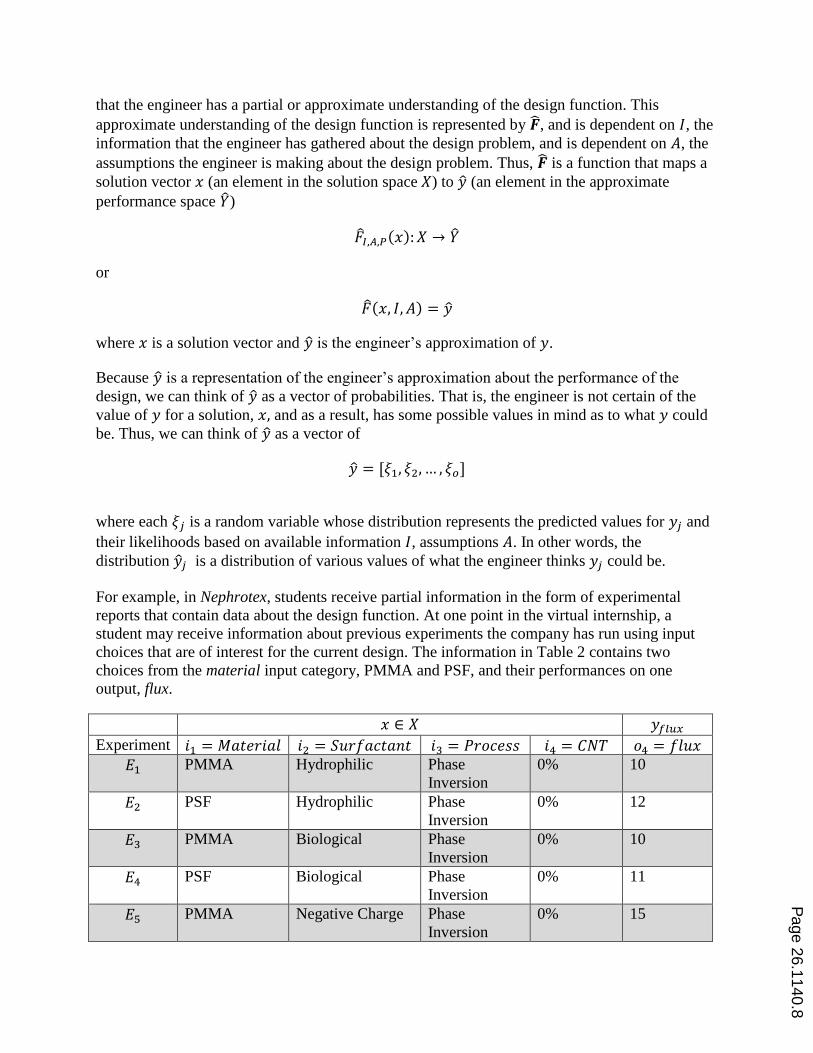
For example, in Nephrotex, students receive partial information in the form of experimental
reports that contain data about the design function. At one point in the virtual internship, a
student may receive information about previous experiments the company has run using input
choices that are of interest for the current design. The information in Table 2 contains two
choices from the material input category, PMMA and PSF, and their performances on one
output, flux.
𝑥 ∈ 𝑋 𝑦𝑓𝑙𝑢𝑥
Experiment 𝑖1 = 𝑀𝑎𝑡𝑒𝑟𝑖𝑎𝑙 𝑖2 = 𝑆𝑢𝑟𝑓𝑎𝑐𝑡𝑎𝑛𝑡 𝑖3 = 𝑃𝑟𝑜𝑐𝑒𝑠𝑠 𝑖4 = 𝐶𝑁𝑇 𝑜4 = 𝑓𝑙𝑢𝑥
𝐸1 PMMA Hydrophilic Phase
Inversion
0% 10
𝐸2 PSF Hydrophilic Phase
Inversion
0% 12
𝐸3 PMMA Biological Phase
Inversion
0% 10
𝐸4 PSF Biological Phase
Inversion
0% 11
𝐸5 PMMA Negative Charge Phase
Inversion
0% 15
Page 26.1140.8

𝐸6 PSF Negative Charge Phase
Inversion
0% 14
Table 2. Information students receive for six experiments for one output, flux in Nephrotex
Each experiment can then be represented as a relationship between 𝑥 and 𝑦. For example, the
first two experiments are:
𝐸1: {𝑥1 = [𝑃𝑀𝑀𝐴, 𝐻𝑦𝑑𝑟𝑜𝑝ℎ𝑖𝑙𝑖𝑐, 𝑃ℎ𝑎𝑠𝑒 𝐼𝑛𝑣𝑒𝑟𝑠𝑖𝑜𝑛, 𝑂%], 𝑦1 = [𝑁𝐴, 𝑁𝐴, 𝑁𝐴, 𝑁𝐴, 𝑦𝑓𝑙𝑢𝑥 = 10]}
𝐸2: {𝑥2 = [𝑃𝑆𝐹, 𝐻𝑦𝑑𝑟𝑜𝑝ℎ𝑖𝑙𝑖𝑐, 𝑃ℎ𝑎𝑠𝑒 𝐼𝑛𝑣𝑒𝑟𝑠𝑖𝑜𝑛, 𝑂%], 𝑦1 = [𝑁𝐴, 𝑁𝐴, 𝑁𝐴, 𝑁𝐴, 𝑦𝑓𝑙𝑢𝑥 = 12]}
And thus, the information that the student has in this case is
𝐼 = {𝐸1, … , 𝐸6}
We have also collected data on the assumptions that students are making while solving design
problems3. One trend that we have seen is that some students assumes separability, that is they
assume that the input choices are independent of one another and do not have an interaction
effect. Thus, the set of assumptions may be represented as
𝐴 = {𝐴1 = 𝑠𝑒𝑝𝑎𝑟𝑎𝑏𝑖𝑙𝑖𝑡𝑦, … , 𝐴𝑛}
With this information and his assumptions, the student may make inferences about the two
materials’ performances. The information he has about the material’s flux performance is
represented in Table 3.
PMMA PSF
𝑦𝑓𝑙𝑢𝑥1 = 10 𝑦𝑓𝑙𝑢𝑥
2 = 12
𝑦𝑓𝑙𝑢𝑥3 = 10 𝑦𝑓𝑙𝑢𝑥
4 = 11
𝑦𝑓𝑙𝑢𝑥5 = 15 𝑦𝑓𝑙𝑢𝑥
6 = 14
Table 3. Student’s understanding of the effects of PMMA and PSF on flux for six experiments
for one output, flux, in Nephrotex
Thus, the student’s understanding of how the materials, PMMA and PSF, perform in terms of
flux can be represented as a distribution:
∀ 𝑥𝑖2∈ 𝐶𝑖2
, 𝑥𝑖3∈ 𝐶𝑖3
, 𝑥𝑖4∈ 𝐶𝑖4
𝑓𝑓𝑙𝑢𝑥([𝑷𝑴𝑴𝑨, 𝑥𝑖2, 𝑥𝑖3
, 𝑥𝑖4], 𝐼, 𝐴) = �̂�𝑓𝑙𝑢𝑥 = {
10, 𝑝 = .66715, 𝑝 = .333
∀ 𝑥𝑖2∈ 𝐶𝑖2
, 𝑥𝑖3∈ 𝐶𝑖3
, 𝑥𝑖4∈ 𝐶𝑖4
𝑓𝑓𝑙𝑢𝑥([𝑷𝑺𝑭, 𝑥𝑖2, 𝑥𝑖3
, 𝑥𝑖4], 𝐼, 𝐴) = �̂�𝑓𝑙𝑢𝑥 = {
11, 𝑝 = .33312, 𝑝 = .33314, 𝑝 = .333
3 It is beyond the scope of this paper to present the detailed student data on assumptions while designing. This
data will be presented in future papers.
Page 26.1140.9

The Valuation Function V
The engineer will then compare elements �̂� to the original functional requirements to determine
if the product is performing according to technical constraints and functional requirements, to the
best of the engineer’s knowledge. However, because each �̂�𝑗 is a probability distribution, an
engineer will typically produce a summary statistic to represent the distribution in order to
compare to the functional requirements and to compare performances between devices. More
specifically, the engineer can calculate one summary statistic for every �̂�𝑗 using a valuation
function, V that maps a vector, �̂� (an element within the space �̂�) to a set of all real numbers
V: �̂� → ℝ𝑂
This function assigns a value 𝑣𝑗(�̂�𝑗), ∀�̂�𝜖�̂�, 𝑗𝜖𝑂 which represents a summary statistic of the
distribution �̂�𝑗. The valuation vector, 𝑣, then contains one value for every element in �̂�.
There are many ways that an engineer might apply a valuation function and calculate the
summary statistic, 𝑣𝑗 . For example, she could calculate the mean, median, or mode of the
distribution or consider the maximum or minimum.
Determining Valuation by Calculating the Mean, Median, Mode, Minimum, or Maximum
In one scenario, an engineer may approach the valuation process by calculating the mean of �̂�𝑗.
Consider the example from Table 3. If the engineer determines the valuation of PMMA by
calculating the mean of the distribution for a solution vector that has PMMA then,
𝑣𝑓𝑙𝑢𝑥(�̂�𝑓𝑙𝑢𝑥 = [10,10,15]) = 11.67
And for a vector that has PSF,
𝑣𝑓𝑙𝑢𝑥(�̂�𝑓𝑙𝑢𝑥 = [12,11,14]) = 12.33
That is, based on the information the engineer has about the design problem, she makes an
inference that the flux of a device that has PMMA as a material choice may be equal to 11.67
and the flux of a device that has PSF as a material may be equal to 12.33.
Determining Valuation from Stated Constraints or Functional Requirements
Now let’s say because of safety concerns, the engineer has a technical constraint of 11 for flux,
meaning that device may not have a flux of less than 11. She may apply a binary function where
if the device passes the threshold, it receives a 1, and if it is less than the threshold, it receives a 0
(Table 4).
Experiment PMMA Passes Threshold
1 10 0
3 10 0
5 15 1
Page 26.1140.10
Experiment PSF Passes Threshold
2 12 1
4 11 1
6 14 1
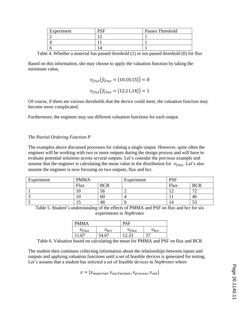
Table 4. Whether a material has passed threshold (1) or not passed threshold (0) for flux
Based on this information, she may choose to apply the valuation function by taking the
minimum value,
𝑣𝑓𝑙𝑢𝑥(�̂�𝑓𝑙𝑢𝑥 = [10,10,15]) = 0
𝑣𝑓𝑙𝑢𝑥(�̂�𝑓𝑙𝑢𝑥 = [12,11,14]) = 1
Of course, if there are various thresholds that the device could meet, the valuation function may
become more complicated.
Furthermore, the engineer may use different valuation functions for each output.
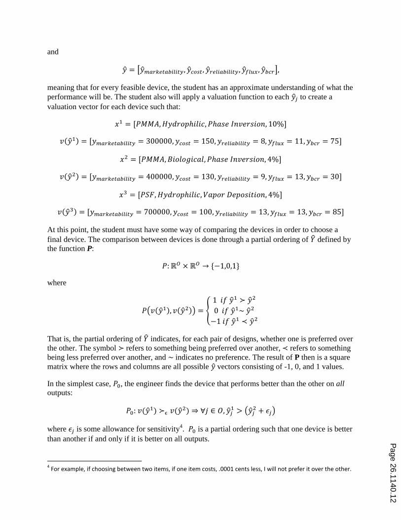
The Partial Ordering Function P
The examples above discussed processes for valuing a single output. However, quite often the
engineer will be working with two or more outputs during the design process and will have to
evaluate potential solutions across several outputs. Let’s consider the previous example and
assume that the engineer is calculating the mean value in the distribution for 𝑣𝑓𝑙𝑢𝑥. Let’s also
assume the engineer is now focusing on two outputs, flux and bcr.
Experiment PMMA Experiment PSF
Flux BCR Flux BCR
1 10 56 2 12 72
3 10 60 4 11 46
5 15 48 6 14 53
Table 5. Student’s understanding of the effects of PMMA and PSF on flux and bcr for six
experiments in Nephrotex
PMMA PSF
𝑣𝑓𝑙𝑢𝑥 𝑣𝑏𝑐𝑟 𝑣𝑓𝑙𝑢𝑥 𝑣𝑏𝑐𝑟
11.67 54.67 12.33 57
Table 6. Valuation based on calculating the mean for PMMA and PSF on flux and BCR
The student then continues collecting information about the relationships between inputs and
outputs and applying valuation functions until a set of feasible devices is generated for testing.
Let’s assume that a student has selected a set of feasible devices in Nephrotex where
𝑥 = [𝑥𝑚𝑎𝑡𝑒𝑟𝑖𝑎𝑙, 𝑥𝑠𝑢𝑟𝑓𝑎𝑐𝑡𝑎𝑛𝑡 , 𝑥𝑝𝑟𝑜𝑐𝑒𝑠𝑠, 𝑥𝑐𝑛𝑡]
Page 26.1140.11
and
�̂� = [�̂�𝑚𝑎𝑟𝑘𝑒𝑡𝑎𝑏𝑖𝑙𝑖𝑡𝑦, �̂�𝑐𝑜𝑠𝑡, �̂�𝑟𝑒𝑙𝑖𝑎𝑏𝑖𝑙𝑖𝑡𝑦 , �̂�𝑓𝑙𝑢𝑥, �̂�𝑏𝑐𝑟],
meaning that for every feasible device, the student has an approximate understanding of what the
performance will be. The student also will apply a valuation function to each �̂�𝑗 to create a
valuation vector for each device such that:
𝑥1 = [𝑃𝑀𝑀𝐴, 𝐻𝑦𝑑𝑟𝑜𝑝ℎ𝑖𝑙𝑖𝑐, 𝑃ℎ𝑎𝑠𝑒 𝐼𝑛𝑣𝑒𝑟𝑠𝑖𝑜𝑛, 10%]
𝑣(�̂�1) = [𝑦𝑚𝑎𝑟𝑘𝑒𝑡𝑎𝑏𝑖𝑙𝑖𝑡𝑦 = 300000, 𝑦𝑐𝑜𝑠𝑡 = 150, 𝑦𝑟𝑒𝑙𝑖𝑎𝑏𝑖𝑙𝑖𝑡𝑦 = 8, 𝑦𝑓𝑙𝑢𝑥 = 11, 𝑦𝑏𝑐𝑟 = 75]
𝑥2 = [𝑃𝑀𝑀𝐴, 𝐵𝑖𝑜𝑙𝑜𝑔𝑖𝑐𝑎𝑙, 𝑃ℎ𝑎𝑠𝑒 𝐼𝑛𝑣𝑒𝑟𝑠𝑖𝑜𝑛, 4%]
𝑣(�̂�2) = [𝑦𝑚𝑎𝑟𝑘𝑒𝑡𝑎𝑏𝑖𝑙𝑖𝑡𝑦 = 400000, 𝑦𝑐𝑜𝑠𝑡 = 130, 𝑦𝑟𝑒𝑙𝑖𝑎𝑏𝑖𝑙𝑖𝑡𝑦 = 9, 𝑦𝑓𝑙𝑢𝑥 = 13, 𝑦𝑏𝑐𝑟 = 30]
𝑥3 = [𝑃𝑆𝐹, 𝐻𝑦𝑑𝑟𝑜𝑝ℎ𝑖𝑙𝑖𝑐, 𝑉𝑎𝑝𝑜𝑟 𝐷𝑒𝑝𝑜𝑠𝑖𝑡𝑖𝑜𝑛, 4%]
𝑣(�̂�3) = [𝑦𝑚𝑎𝑟𝑘𝑒𝑡𝑎𝑏𝑖𝑙𝑖𝑡𝑦 = 700000, 𝑦𝑐𝑜𝑠𝑡 = 100, 𝑦𝑟𝑒𝑙𝑖𝑎𝑏𝑖𝑙𝑖𝑡𝑦 = 13, 𝑦𝑓𝑙𝑢𝑥 = 13, 𝑦𝑏𝑐𝑟 = 85]
At this point, the student must have some way of comparing the devices in order to choose a
final device. The comparison between devices is done through a partial ordering of �̂� defined by
the function P:
𝑃: ℝ𝑂 × ℝ𝑂 → {−1,0,1}
where
𝑃(𝑣(�̂�1), 𝑣(�̂�2)) = {
1 𝑖𝑓 �̂�1 ≻ �̂�2
0 𝑖𝑓 �̂�1~ �̂�2
−1 𝑖𝑓 �̂�1 ≺ �̂�2
That is, the partial ordering of �̂� indicates, for each pair of designs, whether one is preferred over
the other. The symbol ≻ refers to something being preferred over another, ≺ refers to something
being less preferred over another, and ~ indicates no preference. The result of P then is a square
matrix where the rows and columns are all possible �̂� vectors consisting of -1, 0, and 1 values.
In the simplest case, 𝑃0, the engineer finds the device that performs better than the other on all
outputs:
𝑃0: 𝑣(�̂�1) ≻ϵ 𝑣(�̂�2) ⇒ ∀𝑗 ∈ 𝑂, �̂�𝑗1 > (�̂�𝑗
2 + 𝜖𝑗)
where 𝜖𝑗 is some allowance for sensitivity4. 𝑃0 is a partial ordering such that one device is better
than another if and only if it is better on all outputs.
4 For example, if choosing between two items, if one item costs, .0001 cents less, I will not prefer it over the other.
Page 26.1140.12

For example, consider again the three feasible devices selected above from Nephrotex. Using 𝑃0
to compare 𝑣(�̂�2) = [400000,130,9,13,30] and 𝑣(�̂�1) = [300000,150,8,11,75] would yield 1
because 𝑣(�̂�2) performs better on every output5 when compared to 𝑣(�̂�1). However, comparing
𝑣(�̂�2) = [400000,130,9,13,30] and 𝑣(�̂�3) = [700000,100,13,13,85] does not yield a result
because there neither device performs better on all outputs compared to the other. The entire
partial ordering matrix for 𝑃0for this example would be:
𝑣(�̂�1) 𝑣(�̂�2) 𝑣(�̂�3)
𝑣(�̂�1) 0 -1 0
𝑣(�̂�2) 1 0 0
𝑣(�̂�3) 0 0 0
Table 7. Pairwise comparison given criteria that a device is preferred if it performs better on all
outputs.
As seen by the example above, in many design situations there may be solutions that do not yield
a result, and thus this method may not be desirable for many design scenarios.
The next most complex model, 𝑃1, would allow one device to be superior to another on more
than half of the outputs
𝑃1: 𝑣(�̂�1) ≻𝜖,𝛿 𝑣(�̂�2) ⇒ ∑ 𝟙{𝑣𝑗(�̂�𝑗
1)>(𝑣𝑗(�̂�𝑗2)+𝜖𝑗)}
𝑗∈𝑂
> (|𝑂|
2+ 𝛿𝑗)
Using the same example, 𝑣(�̂�3) would be preferred over 𝑣(�̂�1) as demonstrated in Table 8.
Marketability Cost Reliability Flux BCR
𝑣(�̂�1) 300000 150 8 11 75
𝑣(�̂�3) 700000 100 13 13 85
Preference 𝑣(�̂�3) 𝑣(�̂�3) 𝑣(�̂�3) 𝑣(�̂�3) 𝑣(�̂�1)
Table 8. Preference of performance vectors given criteria of performing better on more than half
of the outputs.
∑ 𝟙 {𝑣(�̂�𝑗3)} = 4
𝑗∈𝑂
> ∑ 𝟙
𝑗∈𝑂
{𝑣(�̂�𝑗1)} = 1
While this may be a common decision rule where one device is better on more categories than
another device, it doesn’t account for the fact that there may be certain outputs that may be
weighted as more important than other outputs.
In the next more complex scenario, 𝑃2 calculates a linear combination for every 𝑣𝑗 for every
device with different linear constants, βj, for each 𝑣𝑗:
5 A high marketability, reliability, and flux is desirable, and a low cost and bcr is desirable.
Page 26.1140.13

𝑃2: 𝑣(�̂�1) ≻𝜖 𝑣(�̂�2) ⇒ ∑ βj
𝑗∈𝑂
𝑣𝑗(�̂�𝑗1) > ∑ βj
𝑗∈𝑂
𝑣𝑗(�̂�𝑗2) + 𝜖
Using the same example, let’s assume the engineer considers bcr four times more important than
the other outputs and thus, βbcr = 4 and βmarketability = βflux = βcost = βreliability = 1.
However, before the engineer does a partial ordering where she sums across all 𝑣𝑗 , she must use
another valuation function that converts each 𝑣𝑗 so that they are all on the same scale.
Then let’s assume she applies a ranking (1 = lowest performing, 2 = highest performing)
comparing across devices for each 𝑣𝑗 (Table 9).
Marketability Cost Reliability Flux BCR
𝑣(�̂�1) 1 1 1 1 2
𝑣(�̂�3) 2 2 2 2 1
Table 9. Ranking of outputs for device 1 and 3.
Then, she applies the coefficients, βj and sums across 𝑣𝑗 for each device (Table 10).
Marketability Cost Reliability Flux BCR ∑ βj
𝑗∈𝑂
𝑣𝑗(�̂�𝑗)
𝑣(�̂�1) 1 1 1 1 2*5 14
𝑣(�̂�3) 2 2 2 2 1*5 13
Table 10. Ranking outputs for device 1 and 3 with the weighted sum of the rankings.
In this case, the first device has a score of 14 and the second device has a score of 13.
∑ βj
𝑗∈𝑂
𝑣𝑗(�̂�𝑗1) = 14 > ∑ βj
𝑗∈𝑂
𝑣𝑗(�̂�𝑗3) = 13
And thus, using this method, 𝑣(�̂�1) would be preferred over 𝑣(�̂�3).
In some cases the engineer may not apply a linear combination model and instead apply a more
complex function to the valuation vectors. Model 𝑃3 accounts for this scenario by applying a
function, 𝑢 to the valuation vectors:
𝑃3: 𝑣(�̂�1) ≻𝜖 𝑣(�̂�2) ⇒ 𝑢(𝑣(�̂�1)) > 𝑢(𝑣(�̂�2)) + 𝜖
And finally, there are other cases not accounted for here in which 𝑃4 can be other forms of partial
ordering of 𝑣(�̂�).
The Tractability Function, T
Development of T
Taken together, the functions �̂�, 𝑽, and 𝑷 describe the engineer’s decision making processes.
Based on these processes, we can now explore the complexity of a design problem and how
Page 26.1140.14

solvable the problem is. In particular, we focus on the optimization aspect of measuring the
complexity of a design problem—by examining how difficult is to obtain a device that meets as
many functional requirements as possible.
We define tractability as how solvable the problem is, which is determined by how difficult it is
to obtain a device that meets as many functional requirements as possible. The tractability
function, 𝑻, depends on the number of criteria that the engineer is trying to optimize, the type of
valuation functions and partial ordering functions applied in the design scenario, as well as how
the engineer is determining the quality of devices.
For example, an engineer may use a valuation method where they assign a value based on a
device passing a certain threshold (see table 4), and then apply the partial ordering function (𝑃3),
𝑃3: 𝑣(�̂�1) ≻𝜖 𝑣(�̂�2) ⇒ 𝑢(𝑣(�̂�1)) > 𝑢(𝑣(�̂�2)) + 𝜖
where
𝑢(𝐹(𝑥))=∑ 𝑣𝑗(𝑦𝑗)𝑗∈𝑂
That is, the engineer calculates the quality of a device, 𝑢, by summing over the valuation vector.
The quality score in this case, 𝑢, represents the number of thresholds that the device meets. In
this scenario, if there are many devices in the design space that satisfy the given thresholds,
satisfactory devices are easier to produce, and as a result the problem is relatively simple. If there
are very few devices that satisfy the given thresholds, then the problem becomes more difficult
because satisfactory devices may be difficult to produce.
Thus, we define tractability, 𝑇(𝐹), as the total quality of all devices relative to the maximum
quality achievable. Formally, the function is defined as:
𝑇(𝐹) =∑ 𝑢(𝐹(𝑥))𝑥∈𝑋
𝑈|𝑋|
and where 𝑢(𝐹(𝑥)) represents some function that determines quality and where 𝑈 is the highest
quality solution
𝑈 = max𝑥∈𝑋
(𝑢(𝐹(𝑥)))
Essentially, the tractability function finds each device’s percentage of the maximum possible
quality and then calculates the mean of those percentages. Thus, every design problem has a
tractability value that measures how easy it is to obtain a quality solution. These values range
from a minimum of 0 to a maximum of 1. In the extreme case where tractability equals 1, then
the problem is trivial—that is, every device 𝑥 ∈ 𝑋 achieves the maximum quality, 𝑈. In the most
difficult case, the tractability equals 0 and there are no devices that meet any thresholds. Page 26.1140.15

Support of the Theory from Student Design Work
Identification of V, U, and P in student decision-making
In Nephrotex, we can calculate 𝑻 by considering the specific approach that students use to
determine valuation and how they calculate a score to represent the quality of the device.
For example, one student in Nephrotex executed a ranking system (1=best performing, 3 = worst
performing) and rated each manufacturing process choice, 𝑥𝑝𝑟𝑜𝑐𝑒𝑠𝑠, on four output values, 𝑦𝑓𝑙𝑢𝑥,
𝑦𝑟𝑒𝑙𝑖𝑎𝑏𝑖𝑙𝑖𝑡𝑦, 𝑦𝑏𝑐𝑟, and 𝑦𝑐𝑜𝑠𝑡 (Figure 1). The student then summed across the rankings and
determined a quality score (7, 8, or 9) for each device with that particular manufacturing process.
Thus, the student used a valuation function that assigned rankings and summed up the rankings
(similar to the example given in table 9).
He explained how the ranking method helped him selected a manufacturing process component:
I ranked between the 3 processing methods from 1 to 3 how they rank compared to the
other ones, and I totaled up the scores to see which ones were the lowest, so that would
have the most closest to one. I found the dry jet wet, but I wanted to choose the vapor
deposition one because it was only one off and it had a higher flux rate and it was more
reliable but it was more expensive and had a higher BCR. I guess the only reason I
didn't pick it was for the steric hindrance--it has one of the highest flux and this one
has like the lowest flux so it equaled out to not terrible.
Page 26.1140.16

Figure 1. Student’s system of ranking devices based on information given.
The student’s explanation indicates that the ranking system affected his choice for another input
category, a surfactant called steric hindrance. He justified his manufacturing process choice by
using a ranking system, but also by thinking about the total impact that all input choices would
have on a particular output category, flux.
The same student then compared the devices to the thresholds given by the stakeholders (Figure
2). Each of the 5 hand-written columns represents one device. The student used a system of
partial ordering consisting of smile-emoticons (meets the preferred thresholds) and x’s (does not
meet the preferred threshold). In the middle of the columns, the student summed the number of
smile-emoticons for each device and selected the device in fifth column because it had more
smile-emoticons than any other device. Thus, the student used a 𝑃3 as a partial ordering function
where he summed the valuation rankings to determine a quality value and then compared the
quality score, 𝑢, for each device.
Figure 2. Student’s system of ranking devices to determine if devices met thresholds.
Calculation of T in a Simulated Design Problem
The tractability for the design problem in Nephrotex is the sum of the quality scores for every
possible device divided by the maximum number of thresholds specified by the customer,
multiplied by the total number of devices in the design problem, which represents the maximum
possible quality. The virtual design problem space has 750 total possible solutions and 20
thresholds identified by the customers and stakeholders. Thus, the tractability for the design
problem in Nephrotex is:
𝑇𝑁𝑒𝑝ℎ𝑟𝑜𝑡𝑒𝑥(𝐹) =0 + 0 + 0 … + 17 + 17 + 18
20(750)= .55
Page 26.1140.17

In RescuShell, the other engineering virtual internship, the virtual design problem space has 810
solutions and 15 thresholds identified by the customers and stakeholders. Thus, the tractability
for the design problem in RescuShell is:
𝑇𝑅𝑒𝑠𝑐𝑢𝑆ℎ𝑒𝑙𝑙(𝐹) =4 + 4 + 4 … + 11 + 12 + 12
15(750)= .50
In the case of Nephrotex and RescuShell, we can see that the tractability of the design problems
are similar, but that the design problem in Nephrotex is more tractable than RescuShell, meaning
the problem in RescuShell is more difficult.
We then calculated the mean percentage of thresholds that were met for students in Nephrotex
and RescuShell (Figure 3) for ten groups of students from each virtual internship, where each
group submitted one final device. On average, Nephrotex students’ final devices met more
thresholds than RescuShell students’ final devices t(17.1)=12.7, p<.01.
Figure 3. Mean percentage of thresholds met by students’ final submitted devices. Error bars are
95% confidence intervals.
Conclusion
The results above show a framework for parameterizing and mathematically modeling student
engineers’ design processes. This framework informed the development of an analysis of
decision-making and a tractability function that measured how difficult it is for a student to
optimize over several functional requirements. The tractability function described here is one
method of measuring the complexity of simulated design problems in terms of the optimization
process. In general, measuring the complexity of design problems allows for instructors to assess
the difficulty of problems and in turn, be able to offer design problems of varying complexity to
students at a variety of levels.
Page 26.1140.18

Limitations
Our work on measuring student design processes and determining tractability has been currently
only implemented in virtual internships. Future work includes applying our measurement
techniques to other contexts such as other digital design learning environments or design team
projects in capstone courses. In addition, this work focuses on the decision-making aspect of
engineering design and is suitable for the more structured part of the engineering design process.
We also plan to examine other measures of tractability, such as how different amounts of given
information about of the design function affects the complexity of the problem. Finally, a larger
goal of this research is to develop design problems with various measures of tractability for
implementation into courses at different levels, for the novice first year to the more experienced
senior student.
Acknowledgements
This work was funded in part by the MacArthur Foundation and by the National Science
Foundation through grants DRL-0918409, DRL-0946372, DRL-1247262, DRL-1418288, DUE-
0919347, DUE-1225885, EEC-1232656, EEC-1340402, and REC-0347000. The opinions,
findings, and conclusions do not reflect the views of the funding agencies, cooperating
institutions, or other individuals.
References
[1] C. L. Dym, Engineering Design A Synthesis of Views. Cambridge, MA: Cambridge University Press, 1994.
[2] H. A. Simon, The sciences of the artificial, 3rd ed. Cambridge, MA: MIT Press, 1996.
[3] C. L. Dym, A. Agogino, O. Eris, D. Frey, and L. Leifer, “Engineering design thinking, teaching and
learning,” J. Eng. Educ., vol. 94, no. 1, pp. 103–120, 2005.
[4] C. J. Atman, O. Eris, J. McDonnell, M. E. Cardella, and J. L. Borgford-Parnell, “Engineering Design
Education,” in The Cambridge Handbook of the Engineering Education, A. Johri and B. M. Olds, Eds. New
York, NY: Cambridge University Press, 2014.
[5] S. D. Sheppard, K. Macatangay, A. Colby, and W. M. Sullivan, Educating Engineers. San Francisco, CA:
Jossey-Bass, 2009.
[6] ABET, “Criteria for Accrediting Engineering.” 2014.
[7] L. Harrisberger, R. Heydinger, J. Seeley, and M. Talburtt, Experiential Learning in Engineering Education.
American Society for Engineering Education, 1976.
[8] R. H. Todd, S. P. Magleby, C. D. Sorensen, B. R. Swan, and D. K. Anthony, “A Survey of Capstone
Engineering Courses in North America,” J. Eng. Educ., vol. 84, no. 2, 1995.
[9] S. A. Ambrose and C. H. Amon, “Systematic Design of a First-Year Mechanical Engineering Course at
Carnegie Mellon University,” J. Eng. Educ., vol. 86, no. 2, pp. 173–181, 1997.
[10] D. Knight, L. Carlson, and J. Sullivan, “Improving Engineering Student Retention Through Hands-On,
Team Based, First-Year Design Projects,” in International Conference on Research in Engineering
Education, 2007.
[11] C. L. Dym, “Teaching Design to Freshmen: Style and Content,” J. Eng. Educ., no. October, 1994.
[12] D. Jonassen, J. Strobel, and C. Beng Lee, “Everyday Problem Solving in Engineering: Lessons for
Engineering Educators,” J. Eng. Educ., vol. 95, no. 2, pp. 139–151, 2006.
[13] E. F. Crawley, J. Malmquist, S. Ostlund, and D. Brodeur, Rethinking engineering education: The CDIO
approach. New York, NY: Springer, 2007.
Page 26.1140.19

[14] M. Somerville, D. Anderson, H. Berbeco, J. R. Bourne, J. Crisman, D. Dabby, and Y. Zastavker, “The Olin
College curriculum: Thinking toward the future,” IEEE Trans. Educ., vol. 48, no. 1, pp. 198–205, 2005.
[15] University of Wisconsin-Madison, “UW BME Design,” Department of Biomedical Engineering, 2013.
[Online]. Available: http://bmedesign.engr.wisc.edu/.
[16] W. J. Tompkins, “Implementing design throughout the curriculum,” in Proc. 2006 Annual Conf. of the
Biomedical Engineering, 2006, p. 35.
[17] G. A. Hazelrigg, “A Framework for Decision-Based Engineering Design,” J. Mech. Des., vol. 120, no. 4, pp.
653–658, 1998.
[18] J. von Neumann and O. Morgenstern, Theory of Games and Economic Behavior. Princeton, NJ: Princeton
University Press, 1944.
[19] D. L. Thurston, “Real and Misconceived Limitations to Decision Based Design With Utility Analysis,” J.
Mech. Des., vol. 123, no. 2001, p. 176, 2001.
[20] A. D. Radford and J. S. Gero, “Multicriteria Optimization in Architectural Design,” in Design Optimization,
J. S. Gero, Ed. Orlando, FL: Academic Press, 1985.
[21] D. G. Saari, “Fundamentals and Implications of Decision-Making,” in Decision Making in Engineering
Design, K. E. Lewis, W. Chen, and L. C. Schmidt, Eds. New York, NY: ASME Press, 2006, pp. 35–42.
[22] C. L. Dym, W. H. Wood, and M. J. Scott, “On the Legitimacy of Pairwise Comparisons,” in Decision
Making in Engineering Design, K. E. Lewis, W. Chen, and L. C. Schmidt, Eds. New York, NY: ASME
Press, 2006, pp. 135–143.
[23] N. C. Chesler, A. R. Ruis, W. Collier, Z. Swiecki, G. Arastoopour, and D. W. Shaffer, “A novel paradigm
for engineering education: Virtual internships with individualized mentoring and assessment of engineering
thinking,” J. Biomech. Eng., vol. 137, no. 2, pp. 1–8, 2015.
[24] N. C. Chesler, G. Arastoopour, C. M. D’Angelo, E. A. Bagley, and D. W. Shaffer, “Design of professional
practice simulator for educating and motivating first-year enginnering students.,” Adv. Eng. Educ., vol. 3,
no. 3, pp. 1–29, 2013.
[25] N. P. Suh, “A Theory of Complexity , Periodicity and the Design Axioms,” Res. Eng. Des., no. 11, pp. 116–
131, 1999.
Page 26.1140.20