measuring temperature with thermocouples – a...

Application Note 043

LabVIEW™, Measurement Studio™, NI-DAQ™, ni.com™, and National Instruments™ are trademarks of National Instruments Corporation. Product and company names mentioned herein are trademarks or trade names of their respective companies.

340524D-01 © Copyright 2001 National Instruments Corporation. All rights reserved. February 2001

Measuring Temperature with Thermocouples – a Tutorial

Travis Ferguson

IntroductionOne of the most frequently used temperature transducers is the thermocouple. Thermocouples are very rugged and inexpensive and can operate over a wide temperature range. A thermocouple is created whenever two dissimilar metals touch and the contact point produces a small open-circuit voltage as a function of temperature. This thermoelectric voltage is known as the Seebeck voltage, named after Thomas Seebeck, who discovered it in 1821. The voltage is nonlinear with respect to temperature. However, for small changes in temperature, the voltage is approximately linear, or

where ∆V is the change in voltage, S is the Seebeck coefficient, and ∆T is the change in temperature.

S varies with changes in temperature, however, causing the output voltages of thermocouples to be nonlinear over their operating ranges. Several types of thermocouples are available; these thermocouples are designated by capital letters that indicate their composition according to American National Standards Institute (ANSI) conventions. For example, a J-type thermocouple has one iron conductor and one constantan (a copper-nickel alloy) conductor.

You can monitor thermocouples with versatile PC-based data acquisition systems. Thermocouples have some special signal conditioning requirements, which this note describes. The Signal Conditioning eXtensions for Instrumentation (SCXI) system, depicted in Figure 1, is a signal conditioning front end for measurement devices. SCXI systems are ideal for amplifying, filtering, and even isolating the very low-level voltages that thermocouples generate.

Figure 1. The SCXI Signal Conditioning Front-End System for Plug-In DAQ Devices

∆V S∆T (1)≈

SCXI

1140

Data Transferred

Directly to

Memory

SCXI

Terminal

Blocks

SCXI

Module

SCXI

1140

SCXI

1140

SCXI

1140

SCXI

1140

SCXI

1140

SCXI

1140

SCXI

1140

SCXI

1140

SCXI

1140

SCXI

1140

SCXI

1140

SCXI-1001

MAINFRAME

SCXI

Signals and

Transducers

Data

Acquisition

Device

SCXI1100

SCXI Chassis

Amplified and

Isolated Signals

Application Note 043 2 ni.com

Figure 2. J-Type Thermocouple

Thermocouple CircuitsGeneral CaseTo measure a thermocouple Seebeck voltage, you cannot simply connect the thermocouple to a voltmeter or other measurement system, because connecting the thermocouple wires to the measurement system creates additional thermoelectric circuits.

Consider the circuit illustrated in Figure 2, in which a J-type thermocouple is in a candle flame that has a temperature you want to measure. The two thermocouple wires are connected to the copper leads of a DAQ board. Notice that the circuit contains three dissimilar metal junctions – J1, J2, and J3. J1, the thermocouple junction, generates a Seebeck voltage proportional to the temperature of the candle flame. J2 and J3 each have their own Seebeck coefficient and generate their own thermoelectric voltage proportional to the temperature at the DAQ terminals. To determine the voltage contribution from J1, you need to know the temperatures of junctions J2 and J3 as well as the voltage-to-temperature relationships for these junctions. You can then subtract the contributions of the parasitic thermocouples at J2 and J3 from the measured voltage.

Cold-Junction CompensationThermocouples require some form of temperature reference to compensate for these unwanted parasitic thermocouples. The term cold junction comes from the traditional practice of holding this reference junction at 0 °C in an ice bath. The National Institute of Standards and Technology (NIST) thermocouple reference tables are created with this setup, illustrated in Figure 3.

J1

J3 (+)

J2 (–)To DAQ Board

��

�� Constantan

Iron

Copper��

© National Instruments Corporation 3 Application Note 043

Figure 3. Traditional Temperature Measurement with Reference Junction Held at 0 °C

In Figure 3, the measured voltage depends on the difference in temperatures T1 and Tref; in this case, Tref is 0 °C. Notice that because the voltmeter lead connections are the same temperature, or isothermal (this term is described in detail later in this note), the voltages generated at these two points are equal and opposing. Therefore, the net voltage error added by these connections is zero.

Under these conditions, if the measurement temperature is above 0 °C, a thermocouple has a positive output; if below 0 °C, the output is negative. When the reference junction and the measurement junction are the same temperature, the net voltage is zero.

Although an ice bath reference is accurate, it is not always practical. A more practical approach is to measure the temperature of the reference junction with a direct-reading temperature sensor and subtract the parasitic thermocouple thermoelectric voltage contributions. This process is called cold-junction compensation. You can simplify computing cold-junction compensation by taking advantage of some thermocouple characteristics.

By using the Thermocouple Law of Intermediate Metals and making some simple assumptions, you can see that the voltage the DAQ board measures in Figure 2 depends only on the thermocouple type, the thermocouple voltage, and the cold-junction temperature. The measured voltage is in fact independent of the composition of the measurement leads and the cold junctions, J2 and J3.

According to the Thermocouple Law of Intermediate Metals, illustrated in Figure 4, inserting any type of wire into a thermocouple circuit has no effect on the output as long as both ends of that wire are the same temperature, or isothermal.

Figure 4. Thermocouple Law of Intermediate Metals

��

Copper

Metal 1

Metal 2��

T1Voltmeter

��

��+

–

IsothermalRegion Ice Bath

Tref = 0° C

��

��

Metal A Metal C

�� =

Metal A Metal B Metal C

��

IsothermalRegion

��


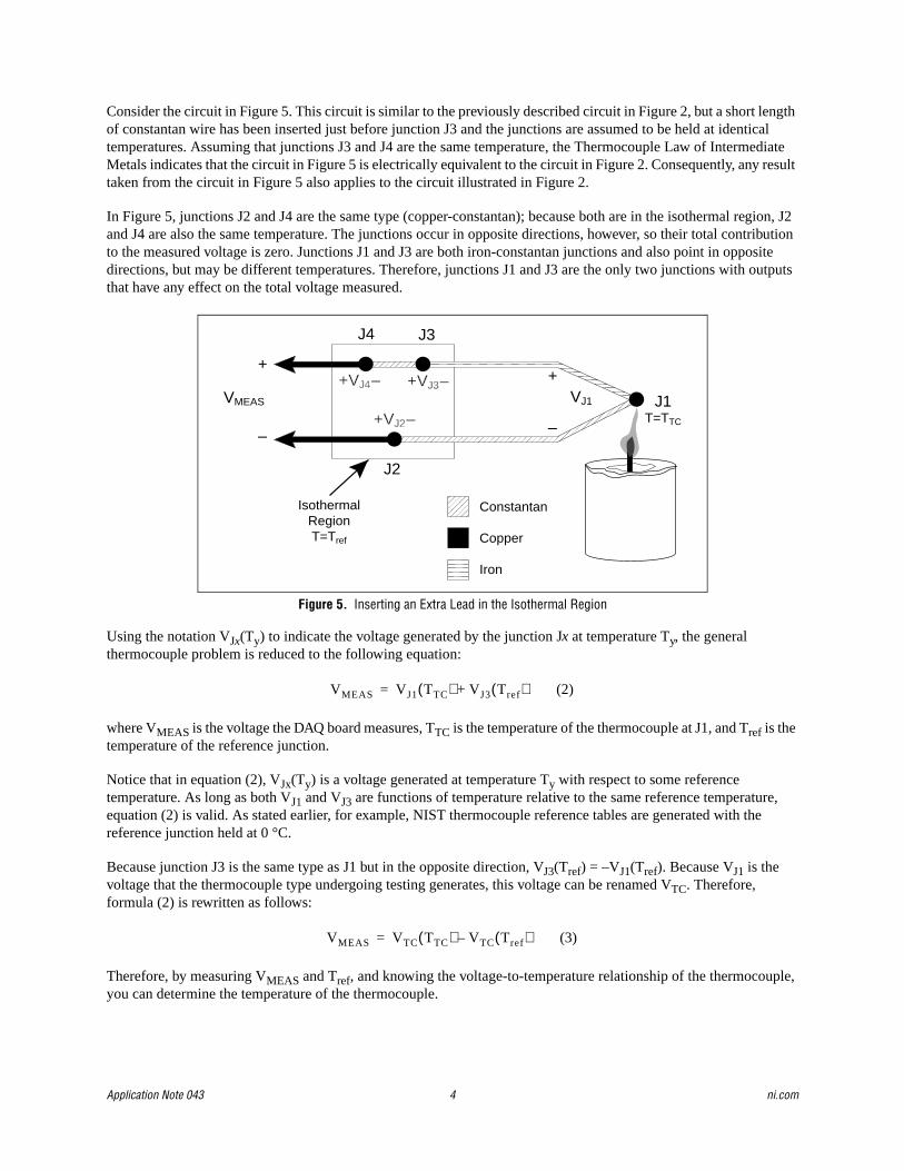
Consider the circuit in Figure 5. This circuit is similar to the previously described circuit in Figure 2, but a short length of constantan wire has been inserted just before junction J3 and the junctions are assumed to be held at identical temperatures. Assuming that junctions J3 and J4 are the same temperature, the Thermocouple Law of Intermediate Metals indicates that the circuit in Figure 5 is electrically equivalent to the circuit in Figure 2. Consequently, any result taken from the circuit in Figure 5 also applies to the circuit illustrated in Figure 2.

In Figure 5, junctions J2 and J4 are the same type (copper-constantan); because both are in the isothermal region, J2 and J4 are also the same temperature. The junctions occur in opposite directions, however, so their total contribution to the measured voltage is zero. Junctions J1 and J3 are both iron-constantan junctions and also point in opposite directions, but may be different temperatures. Therefore, junctions J1 and J3 are the only two junctions with outputs that have any effect on the total voltage measured.

Figure 5. Inserting an Extra Lead in the Isothermal Region

Using the notation VJx(Ty) to indicate the voltage generated by the junction Jx at temperature Ty, the general thermocouple problem is reduced to the following equation:

where VMEAS is the voltage the DAQ board measures, TTC is the temperature of the thermocouple at J1, and Tref is the temperature of the reference junction.

Notice that in equation (2), VJx(Ty) is a voltage generated at temperature Ty with respect to some reference temperature. As long as both VJ1 and VJ3 are functions of temperature relative to the same reference temperature, equation (2) is valid. As stated earlier, for example, NIST thermocouple reference tables are generated with the reference junction held at 0 °C.

Because junction J3 is the same type as J1 but in the opposite direction, VJ3(Tref) = –VJ1(Tref). Because VJ1 is the voltage that the thermocouple type undergoing testing generates, this voltage can be renamed VTC. Therefore, formula (2) is rewritten as follows:

Therefore, by measuring VMEAS and Tref, and knowing the voltage-to-temperature relationship of the thermocouple, you can determine the temperature of the thermocouple.

��Constantan

Copper

Iron��

J1T=TTC

J3

J2

VMEAS

��+

–

J4

IsothermalRegionT=Tref

+

–

VJ1

VJ3+ –VJ4+ –

VJ2+ –

��

VMEAS VJ1 TTC( ) VJ3 Tref( ) (2)+=

VMEAS VTC TTC( ) VTC Tref( ) (3)–=


There are two techniques for implementing cold-junction compensation – hardware compensation and software compensation. Both techniques require that the temperature at the reference junction be sensed with a direct-reading sensor. A direct-reading sensor has an output that depends only on the temperature of the measurement point. Semiconductor sensors, thermistors, or RTDs are commonly used to measure the reference-junction temperature. For example, several SCXI terminal blocks include thermistors that are located near the screw terminals to which thermocouple wires are connected.

Hardware CompensationWith hardware compensation, a variable voltage source is inserted into the circuit to cancel the parasitic thermoelectric voltages. The variable voltage source generates a compensation voltage according to the ambient temperature, and thus adds the correct voltage to cancel the unwanted thermoelectric signals. When these parasitic signals are canceled, the only signal the DAQ system measures is the voltage from the thermocouple junction. With hardware compensation, the temperature at the DAQ system terminals is irrelevant because the parasitic thermocouple voltages have been canceled. The major disadvantage of hardware compensation is that each thermocouple type must have a separate compensation circuit that can add the correct compensation voltage, which makes the circuit fairly expensive. Also, hardware compensation is generally less accurate than software compensation.

Software CompensationAlternatively, you can use software for cold-junction compensation. After a direct-reading sensor measures the reference-junction temperature, software can add the appropriate voltage value to the measured voltage to eliminate the parasitic thermocouple effects. Recall formula (3), which states that the measured voltage, VMEAS, is equal to the difference between the thermocouple voltages at the thermocouple temperature and at the reference-junction temperature.

Note National Instruments NI-DAQ driver software, as well as National Instruments LabVIEW and Measurement Studio application environments, include built-in routines that perform the required software compensation.

There are two ways to determine the thermocouple temperature when given the measured voltage, VMEAS, and the temperature at the reference junction, Tref. The first method is more accurate, but the second method requires fewer computational steps.

Procedure 1 – Direct Voltage Addition Method for Software Cold-Junction CompensationThe more accurate compensation method uses two voltage-to-temperature conversion steps. From formula (3), you can find the true open-circuit voltage that the thermocouple would produce with a reference junction at 0 °C, as shown in the following equation:

Therefore, this method requires the following steps:

1. Measure the reference-junction temperature, Tref.

2. Convert this temperature into an equivalent voltage for the thermocouple type undergoing testing, VTC(Tref). You can use either the NIST reference tables or polynomials that assume a reference junction at 0 °C.

3. Add this equivalent voltage to the measured voltage, VMEAS, to obtain the true open-circuit voltage that the thermocouple would produce with a reference junction at 0 °C, VTC(TTC).

4. Convert the resulting voltage into a temperature; this value is the thermocouple temperature, TTC.

This compensation method requires a translation of the junction temperature into a thermocouple voltage followed by a translation of a new voltage into a temperature. Each of these translation steps requires either a polynomial calculation or a look-up table. It is, however, more accurate than the following method.

VTC TTC( ) VMEAS VTC Tref( ) (4)+=


Procedure 2 – Temperature Addition Method for Software Cold-Junction CompensationA second, easier software compensation approach makes use of the fact that thermocouple output voltages are approximately linear over small deviations in temperature. Therefore, for small deviations in temperature, you can use the following equation:

This assumption is true if T1 is fairly close to T2 because the thermocouple voltage-versus-temperature curve is approximately linear for small temperature variations. Assuming that the thermocouple temperature is relatively close to the reference temperature, you can rewrite formula (3) as shown in the following equation:

Remember that if you are using standard NIST thermocouple reference tables or equations, the voltage VTC is a function of temperature relative to a reference temperature of 0 °C. By assuming linearity and using equation (6), assume that the voltage-versus-temperature curves with a reference temperature of 0 °C are identical to curves with a reference temperature of Tref. Therefore, you can convert the measured voltage into a temperature using the NIST reference tables. This temperature is the difference between temperatures TTC and Tref. This simplified compensation method is as follows:

1. Measure the reference-junction temperature, Tref.

2. Convert the measured voltage, VMEAS, into a temperature using the voltage-to-temperature relationship of the thermocouple. This temperature is approximately the difference between the thermocouple and the cold-junction reference, TTC – Tref.

3. Add the temperature of the reference junction, Tref, to this value. This is the thermocouple temperature.

This method saves a computation step over the first method of software compensation but is less accurate. A comparison of the accuracy of these two methods is included in the application examples later in this note.

Linearizing the DataThermocouple output voltages are highly nonlinear. The Seebeck coefficient can vary by a factor of three or more over the operating temperature range of some thermocouples. For this reason, you must either approximate the thermocouple voltage-versus-temperature curve using polynomials, or use a look-up table. The polynomials are in the following form:

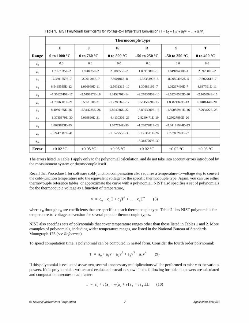
where v is the thermocouple voltage in volts, T is the temperature in degrees Celsius, and a0 through an are coefficients that are specific to each thermocouple type. Table 1 lists NIST polynomial coefficients for several popular thermocouple types over a selected range of temperature.

VTC T1( ) VTC T2( )– VTC T1 T2–( ) (5)≈

VMEAS VTC TTC Tref–( ) (6)=

T a0 a1v a2v2 ... anvn (7)+ + + +=


The errors listed in Table 1 apply only to the polynomial calculation, and do not take into account errors introduced by the measurement system or thermocouple itself.

Recall that Procedure 1 for software cold-junction compensation also requires a temperature-to-voltage step to convert the cold-junction temperature into the equivalent voltage for the specific thermocouple type. Again, you can use either thermocouple reference tables, or approximate the curve with a polynomial. NIST also specifies a set of polynomials for the thermocouple voltage as a function of temperature,

where c0 through cn are coefficients that are specific to each thermocouple type. Table 2 lists NIST polynomials for temperature-to-voltage conversion for several popular thermocouple types.

NIST also specifies sets of polynomials that cover temperature ranges other than those listed in Tables 1 and 2. More examples of polynomials, including wider temperature ranges, are listed in the National Bureau of Standards Monograph 175 (see Reference).

To speed computation time, a polynomial can be computed in nested form. Consider the fourth order polynomial:

If this polynomial is evaluated as written, several unnecessary multiplications will be performed to raise v to the various powers. If the polynomial is written and evaluated instead as shown in the following formula, no powers are calculated and computation executes much faster:

Table 1. NIST Polynomial Coefficients for Voltage-to-Temperature Conversion (T = a0 + a1v + a2v2 + ... + anvn)

Thermocouple Type

E J K R S T

Range 0 to 1000 °C 0 to 760 °C 0 to 500 °C –50 to 250 °C –50 to 250 °C 0 to 400 °C

a0 0.0 0.0 0.0 0.0 0.0 0.0

a1 1.7057035E–2 1.978425E–2 2.508355E–2 1.8891380E–1 1.84949460E–1 2.592800E–2

a2 –2.3301759E–7 –2.001204E–7 7.860106E–8 –9.3835290E–5 –8.00504062E–5 –7.602961E–7

a3 6.5435585E–12 1.036969E–11 –2.503131E–10 1.3068619E–7 1.02237430E–7 4.637791E–11

a4 –7.3562749E–17 –2.549687E–16 8.315270E–14 –2.2703580E–10 –1.52248592E–10 –2.165394E–15

a5 –1.7896001E–21 3.585153E–21 –1.228034E–17 3.5145659E–13 1.88821343E–13 6.048144E–20

a6 8.4036165E–26 –5.344285E–26 9.804036E–22 –3.8953900E–16 –1.59085941E–16 –7.293422E–25

a7 –1.3735879E–30 5.099890E–31 –4.413030E–26 2.8239471E–19 8.23027880E–20

a8 1.0629823E–35 1.057734E–30 –1.2607281E–22 –2.34181944E–23

a9 –3.2447087E–41 –1.052755E–35 3.1353611E–26 2.79786260E–27

a10 –3.3187769E–30

Error ±0.02 °C ±0.05 °C ±0.05 °C ±0.02 °C ±0.02 °C ±0.03 °C

v co c1T c2T2 ... cnTn (8)+ + + +=

T a0 a1v a2v2 a3v3 a4v4 (9)+ + + +=

T a0 v a1 v a2 v a3 va4+( )+( )+( ) (10)+=


These NIST polynomials are implemented in functions included with LabVIEW, LabWindows/CVI, and NI-DAQ software from National Instruments.

Note As a precaution, check the units specified for the voltages. For the formulas in Tables 1 and 2, the voltages are in microvolts. For some other thermocouple tables and linearization polynomials, the voltages may be in millivolts or volts. Using the incorrect unit yields erroneous results.

Critical Technologies for Thermocouple MeasurementsThe following sections describe some general measurement capabilities that can be important when measuring temperatures with thermocouples

Low-Noise SystemLow-level thermocouple signals are very susceptible to noise corruption. Therefore, it is very important that your measurement products are well shielded with very good low-noise performance. National Instruments measurement products are designed to prevent signal corruption from external noise. For example, the SCXI front-end signal conditioning system consists of fully shielded chassis and modules. Signals are passed along a low-noise analog bus and then to a plug-in data acquisition device via a shielded, twisted-pair cable for the best possible low-noise performance.

Table 2. NIST Polynomial Coefficients for Temperature-to-Voltage Conversion (v = c0 + c1T + c2T2 + ... + cnTn)

Thermocouple Type

E J K R S T

Range 0 to 1000 °C –210 to 760 °C 0 to 1372 °C –50 to 1064 °C –50 to 1064 °C 0 to 400 °C

c0 0.0 0.0 –17.600413686 0.0 0.0 0.0

c1 58.665508710 50.38118782 38.921204975 5.28961729765 5.40313308631 38.748106364

c2 4.503227558E–2 3.047583693E–2 1.85587700E–2 1.3916658978E–2 1.2593428974E–2 3.32922279E–2

c3 2.890840721E–5 –8.56810657E–5 –9.9457593E–5 –2.388556930E–5 –2.324779687E–5 2.06182434E–4

c4 –3.30568967E–7 1.322819530E–7 3.18409457E–7 3.5691600106E–8 3.2202882304E–8 –2.18822568E–6

c5 6.50244033E–10 –1.7052958E–10 –5.607284E–10 –4.62347666E–11 –3.314651964–11 1.09968809E–8

c6 –1.9197496E–13 2.09480907E–13 5.6075059E–13 5.007774410E–14 2.557442518E–14 –3.0815759E–11

c7 –1.2536600E–15 –1.2538395E–16 –3.202072E–16 –3.73105886E–17 –1.25068871E–17 4.54791353E–14

c8 2.14892176E–18 1.56317257E–20 9.7151147E–20 1.577164824E–20 2.714431761E–21 –2.7512902E–17

c9 –1.4388042E–21 –1.210472E–23 –2.81038625E–24

c10 3.59608995E–25 NOTE A

NOTE A: The equation for type K is v c0 c1T c2T2 ... c9Tn 118.5976e(–1.183432E–4)(T – 126.9686)2

+ + + + +=


Figure 6. SCXI Front-End Signal Conditioning

You can also improve the noise performance of your system significantly by amplifying the low-level thermocouple voltages as close as possible to the thermocouple. Until the thermocouple signal is amplified, this low-level voltage is susceptible to noise from the surrounding environment. Many times the level of noise is comparable to or greater than the thermocouple signal itself. To make matters worse, thermocouple wire acts as an antenna picking up this noise. However, once you have amplified the thermocouple signal, your signal is typically several orders of magnitude greater than the noise source, thus reducing or eliminating the effects of the noise on your measurement.

AmplificationBecause thermocouple output voltages are very low, you should use as large a gain as possible for the best resolution and noise performance. Amplification, together with the input range of your analog-to-digital converter (ADC), determines the usable input range of your system. Therefore, you should carefully select your amplification so that the thermocouple signal does not exceed this range at elevated temperatures.

Table 3 lists the voltage ranges from several standard thermocouple types; you can use this table as a guide for determining the best input-range settings to use.

Table 3. Thermocouple Voltage Output Extremes (mV)

Thermocouple Type

ConductorTemperature Range (°C)

Voltage Range (mV)

Seebeck Coefficient

(µV/°C)Positive Negative

E Chromel Constantan –270 to 1,000 –9.835 to 76.358 58.70 at 0 °C

J Iron Constantan –210 to 1,200 –8.096 to 69.536 50.37 at 0 °C

K Chromel Alumel –270 to 1,372 –6.548 to 54.874 39.48 at 0 °C

T Copper Constantan –270 to 400 –6.258 to 20.869 38.74 at 0 °C

SPlatinum-10%

Rhodium Platinum –50 to 1,768 –0.236 to 18.698 10.19 at 600 °C

RPlatinum-13%

Rhodium Platinum –50 to 1,768 –0.226 to 21.108 11.35 at 600 °C


Input FilteringTo further reduce noise, consider a measurement system with a lowpass resistor-capacitor (RC) filter on each input channel, typically 1 to 4 Hz. These are useful for removing the 50/60 Hz power line noise prevalent in most laboratory and plant settings. For high-rate scanning applications, you may want to consider choosing a solution that applies a filter per channel, rather than an architecture that multiplexes many channels into a single filter. Architectures that multiplex numerous channels through a single filter can reduce your overall system scanning rate.

Open Thermocouple DetectionIt is useful to detect a break, or open circuit, in a thermocouple circuit. Otherwise, you may be unaware that data you are acquiring is actually incorrect, due to a broken thermocouple. Many measurement systems use technologies that cause an input channel to saturate at its full-scale positive or full-scale negative value if the input leads are an open circuit. Your measurement system will then report a value of full-scale output in either direction. You can check for this condition with software and take the necessary action.

Cold-Junction CompensationAs discussed earlier, thermocouple measurements require sensing of the cold-junction (or reference) temperature at the point where the thermocouple wire is connected to the measurement system. Therefore, signal connection accessories should include an accurate cold-junction sensor and be designed to minimize temperature gradients between the cold-junction sensor and thermocouple wire connections.

Depending on the measurement system you choose, you typically have several options when selecting your cold-junction compensation technology. Some systems use the National Semiconductor LM-35CAZ temperature sensor as a reference. These products generate a linear voltage output of 10 mV/°C. Other options provide a high-precision thermistor to measure the cold-junction temperature. These same products typically offer an isothermal plate that helps maintain all screw terminals and the thermistor at the same temperature. With these solutions, you can measure the reference temperature with 0.5 °C accuracy.

ScanningThermocouple systems are generally low-bandwidth applications, because temperature is typically a slow-changing process. However, there are times when you may need a high-speed measurement system, depending on your system size and inputs from sensors other than thermocouples. For example, a 10 Hz scanner monitoring 300 thermocouples can sample each thermocouple only once every 30 s. An SCXI system, which can scan input channels at up to 3 µs per channel, can sample all 300 thermocouples every 0.9 ms. Another reason for a high scanning rate is to simulate simultaneous sampling. Even though you may only want to read each channel once every 10 s, you may need to minimize the sampling delays between each channel. Finally, you may consider high-speed scanning systems when thermocouples are not the only type of signal you are measuring. Measuring temperatures at the same time as other higher-frequency signals such as vibration may require you to measure all channels at the same rate.

Differential MeasurementsIf you are using any grounded thermocouples, differential measurement is important. With differential measurements, each channel uses two signal leads; only the voltage difference between the leads is measured. The differential amplifier rejects ground-loop noise and common-mode noise, which therefore do not corrupt the measurement. With single-ended measurements, on the other hand, the negative leads of all the input signals are connected to a common ground. While this can increase the channel count of your measurement system, this also increases the likelihood of ground loops, and you do not gain the common-mode rejection capabilities of differential measurements.


IsolationAlthough a thermocouple signal is very small, the thermocouple itself may be exposed to large common-mode voltages. For example, if you connect a thermocouple to the windings of a motor, the common-mode signal to your measurement device can be several hundred volts. Measurement systems with isolation are built to block these larger common-mode voltage levels, as well as adding system protection to voltage spikes or improper signal connections.

Thermocouple Measurement System OptionsNational Instruments offers a variety of computer-based measurement options that offer increased system performance, tighter integration with other measurement hardware and software, and better development tools, all at a lower cost than traditional systems.

SCXISCXI is a front-end signal conditioning and switching system for various measurement devices, including plug-in data acquisition and DMM devices. An SCXI system consists of a rugged chassis that houses shielded signal conditioning modules that amplify, filter, isolate, and multiplex analog signals from thermocouples or other transducers. SCXI is designed for large measurement systems or systems requiring high-speed acquisition.

System features include:

• Modular architecture – choose your measurement technology

• Expandability – expand your system to 3,072 channels

• Integration – combine analog input, analog output, digital I/O, and switching into a single, unified platform

• High bandwidth – acquire signals at an aggregate rate up to 333 kHz

• Connectivity – select from SCXI modules with thermocouple connectors or terminal blocks

For complete information about the SCXI product line, please visit ni.com/sigcon

SCCSCC is a front-end signal conditioning system for E Series plug-in data acquisition devices. An SCC system consists of a shielded carrier that holds up to 20 single or dual-channel SCC modules for conditioning thermocouples and other transducers. SCC is designed for small measurement systems where you need only a few channels of each signal type, or for portable applications. SCC systems also offer the most comprehensive and flexible signal connectivity options.


• Modular architecture – select your measurement technology on a per-channel basis

• Small-channel systems – condition up to 16 analog input and eight digital I/O lines

• Low-profile/portable – integrates well with other laptop computer measurement technologies

• High bandwidth – acquire signals at rates up to 1.25 MHz

• Connectivity – incorporates panelette technology to offer custom connectivity to thermocouple, BNC, LEMO® (B Series), and MIL-Spec connectors

For complete information about the SCC product line, visit ni.com/sigcon

5B Series5B is a front-end signal conditioning system for plug-in data acquisition devices. A 5B system consists of eight or 16 single-channel modules that plug into a backplane for conditioning thermocouples and other analog signals. National Instruments offers a complete line of 5B modules, carriers, backplanes, and accessories. For more information, visit ni.com/sigcon


FieldPointFieldPoint is a distributed measurement system for monitoring or controlling signals in light industrial applications. A FieldPoint system includes a serial or Ethernet network module and up to nine I/O modules in a bank. Each I/O module can measure eight or 16 channels. FieldPoint is designed for applications with small clusters of I/O points at several different locations. FieldPoint is also an attractive solution for cost-sensitive applications performing low-speed monitoring.


• Modular architecture – select your measurement technology on a per-module basis

• Expandability – network multiple banks to a single system

• Integration – combine analog input, analog output, digital I/O, and switching into a single, unified platform

• Low-speed monitoring – up to 100 Hz

• Light-industrial grade – 70 °C temperature range, hot-swappable, programmable start-up states, watchdog timers.

For complete information about the FieldPoint product line, please visit ni.com/fieldpoint

NI 4350 Precision LoggersThe NI 4350 Series consists of precision digitizers designed specifically for temperature, resistance, and low-frequency analog measurements. An NI 4350 system consists of a plug-in device, cable, and signal connection accessory. Choose an NI 4350 Series device as part of your solution when you need high-accuracy measurements at low acquisition rates (up to 60 Hz).


• High-accuracy – 24-bit ADCs with digital filtering to reject 50/60 Hz noise

• Platform options – available for PCI, PXI/CompactPCI, USB, PCMCIA, and ISA

• Small-channel-count systems – measure up to 14 thermocouples per device

• Low-speed monitoring – maximum scanning rate of 60 Hz

For complete information about the NI 4350 series product line, please visit ni.com/instruments/loggers

Sources of ErrorWhen making thermocouple measurements, possible sources of error include compensation, linearization, measurement, thermocouple wire, and experimental errors.

Cold-junction compensation errors arise from two sources – inaccuracy of the temperature sensor and temperature differences between the sensor and the screw terminals. Cold-junction compensation sensors that are IC based have an effective accuracy of ±0.9 °C. In addition, temperature gradients between the sensor and the screw terminals can be as high as ±0.5 °C, for a total accuracy of ±1.4 °C. Other solutions use an isothermal design to limit temperature gradients and a high-precision thermistor to achieve accuracy as low as ±0.65 °C.

Linearization errors occur because polynomials are approximations of the true thermocouple output. Linearization error depends on the degree of the polynomial used. Table 1 lists the linearization errors for the NIST polynomials.

Measurement error is the result of inaccuracies in the digitizer and signal conditioning technologies of your measurement device. These include offset error, gain error, nonlinearities, and resolution of the ADC. Although National Instruments products are calibrated to minimize offset errors, you can completely remove the offset error of any product by grounding the input, taking a reading, and subtracting this offset error from subsequent readings. Some products offer this feature automatically.


The amplifiers in your measurement system can also introduce gain error. For example, a system gain error of 0.03 percent can result in a 6 mV error, depending on gain settings. However, you can use an external calibration source to remove this gain error completely.

Other sources of measurement error include the nonlinearity and resolution of the digitizer. These errors are typically minimized by the high gain associated with thermocouple measurement products.

Often, the major source of error is the thermocouple itself. Thermocouple wire error, for example, is caused by inhomogeneity in the thermocouple manufacturing process. These errors vary widely depending on the thermocouple type and even the gauge of wire used, but a value of ±2 °C is typical. Check with the thermocouple manufacturer for exact accuracy specifications. A common practice to combat this error is to purchase a spool of thermocouple wire and make your own thermocouples. This ensures measurement consistency between your thermocouples. Then, if you calibrate your system to one of the thermocouples, you have calibrated your system to all of your thermocouples.

Another potential source of error is noise picked up by the thermocouple leads. Lowpass filtering is your most effective method to combat noise, but software averaging can also remove noise from your measurements.

ConclusionThermocouples are inexpensive temperature sensing devices, widely used with computer-based measurement systems. Thermocouple measurement requires specific signal conditioning technologies, including cold-junction compensation, amplification, and linearization. Consider additional signal conditioning technologies such as lowpass filtering, isolation, and isothermal design, when appropriate. National Instruments offers many different thermocouple measurement solutions, including SCXI, SCC, and 5B front-end signal conditioning for data acquisition devices, FieldPoint for distributed/light industrial applications, and data loggers for precision measurements.

ReferenceG. W. Burns, M. G. Scroger, G. F. Strouse, et al. Temperature-Electromotive Force Reference Functions and Tables for the Letter-Designated Thermocouple Types Based on the IPTS-90 NIST Monograph 175. Washington, D.C.: U.S. Department of Commerce, 1993.

measuring temperature with thermocouples – a...

Documents