Mm

JHa

b

c

a

ARRA

KALLAY

1

chtaaBityiitt

c

T

0d

Ecological Modelling 232 (2012) 109– 118

Contents lists available at SciVerse ScienceDirect

Ecological Modelling

jo ur n al homep ag e: www.elsev ier .com/ locate /eco lmodel

easuring agricultural land-use intensity – A global analysis using aodel-assisted approach

an Philipp Dietricha,b,∗, Christoph Schmitza,c, Christoph Müllera, Marianela Fadera,ermann Lotze-Campena, Alexander Poppa

Potsdam Institute of Climate Impact Research (PIK), Telegraphenberg A 31, 14473 Potsdam, GermanyDepartment of Physics, Humboldt University, Newtonstr. 15, 12489 Berlin, GermanyDepartment of Agricultural Economics and Social Sciences, Humboldt University, Philippstr. 13, 10115 Berlin, Germany

r t i c l e i n f o

rticle history:eceived 28 November 2011eceived in revised form 28 February 2012ccepted 1 March 2012

eywords:

a b s t r a c t

Human activities such as research & development, infrastructure or management are of major importancefor agricultural productivity. These activities can be summarized as agricultural land-use intensity. Wepresent a measure, called the �-factor, which is an alternative to current measures for agricultural land-use intensity. The �-factor is the ratio between actual yield and a reference yield under well definedmanagement and technology conditions. By taking this ratio, the physical component (soils, climate),

gricultureand-use intensityand-usegricultural productivityield growth

which is equal in both terms, is removed. We analyze global patterns of agricultural land-use intensityfor 10 world regions and 12 crops, employing reference yields as computed with a global crop growthmodel for the year 2000. We show that parts of Russia, Asia and especially Africa had low agriculturalland-use intensities, whereas the Eastern US, Western Europe and parts of China had high agriculturalland-use intensities in 2000. Our presented measure of land use intensity is a useful alternative to existingmeasures, since it is independent of socio-economic data and allows for quantitative analysis.

© 2012 Elsevier B.V. All rights reserved.

. Introduction

Future demand for agricultural products will increase over theoming decades, driven by population growth and changing dietaryabits (Pingali, 2007; von Braun, 2007), which means that agricul-ural production will have to increase. The two basic options for thisre expansion of the land area under agricultural production, andgricultural land-use intensification (for definitions see Table 1).ecause land expansion is limited (Lambin and Meyfroidt, 2011),

ntensification has been and will increasingly become more impor-ant in the future (Ewert et al., 2005). To assess further long-termield growth and for projections of future land-use developmentst is essential to quantify current levels of agricultural land-usentensity, assuming that further improvements are more difficulto achieve in systems operating at the forefront of intensity levels

han for systems at lower intensity levels (e.g. spillover).

Literature provides two different concepts for analyzing agri-ultural performance: yield gap analysis and analysis of land-use

∗ Corresponding author at: Potsdam Institute of Climate Impact Research (PIK),elegraphenberg A 31, 14473 Potsdam, Germany.

E-mail address: dietrich@pik-potsdam.de (J.P. Dietrich).

304-3800/$ – see front matter © 2012 Elsevier B.V. All rights reserved.oi:10.1016/j.ecolmodel.2012.03.002

intensities.1 Yield gap analyses assume that each location has anupper yield boundary, called either “potential yield” (Ittersum andRabbinge, 1997) or “technology frontier” (Nishimizu and Page,1982), which is determined by present physical conditions andavailable technologies. Observed or actual yields may be lower thanthe potential yield due to the ineffective application of inputs andavailable technologies. Regions with strong discrepancies betweenactual and potential yield have strong potentials for further yieldincreases, whereas regions at the technology frontier are not ableto increase their yields any further (Färe et al., 1994; Coelli andRao, 2005; Neumann et al., 2010). This approach can be seen as ashort-term analysis of agricultural potentials, since it focuses onagricultural inputs and management, which can be changed andoptimized within years. However, it excludes productivity changesinduced by Research & Development (R&D) (Licker et al., 2010;Johnston et al., 2011), which typically have a time lag of around

10–30 years (Alston et al., 1995, 2000).

The concept of agricultural land-use intensity as followed in thispaper does not measure the distance to a technology frontier or

1 In this paper we use the term land use intensity analysis contrasting to yield gapanalysis rather than a generic term for agricultural potential analysis as it is some-times used in literature. For further explanations for this choice check AppendixD.

110 J.P. Dietrich et al. / Ecological Mod

Table 1Concepts and terms used in this paper.

Concept Description

Yield A measure of the output per unit areaHuman activity Any kind of human interaction influencing

yields (e.g. management or R&D)Physical environment Natural circumstances under which

production takes place (soil, climate, terrain)Agricultural land-useintensity ˛

Degree of yield amplification caused by humanactivities

po1tvGwtboiwactDtAba(dsa

ooiotilo(iciflo

opieIa2uf

ap

�-Factor Measure proportional to agricultural land-useintensity

otential yield. Instead, it is a productivity measure which takesnly the human-induced productivity into account (Brookfield,993; Kates et al., 1993; Netting, 1993), explicitly including thosehat affect the technology frontier like the development of newarieties as during the so-called green revolution (Evenson andollin, 2003). Although, both measures can be calculated in similarays, their meaning is different: yield gap measures the distance to

he currently best practice, typically excluding possible changes inest practices, whereas land-use intensity measures all those partsf agricultural productivity, which cannot be explained by the phys-cal environment (soils, climate). This difference becomes eminent

hen comparing values at different time steps. A farm not adoptingny technological progress will show an increasing yield gap, butonstant land-use intensity. This is, because the technology fron-ier moves in this case, but not the productivity level (see Appendix

for more details on this example and more explanations abouthe crucial differences between yield gap and land use intensity).s the position of the technology frontier cannot be assumed toe constant over decades, measures of land-use intensity are moredequate tools for assessing long-term developments in agriculturetime horizons of several decades). Due to its more comprehensiveefinition with respect to yield increasing activities, land-use inten-ity is also more appropriate as a surrogate for the general state ofgricultural development.

The concept “land-use intensity” is less clearly defined than thatf yield gap analysis. Sometimes the term is used in the sense of anverarching definition, including yield gap analysis as some part oft, in other cases it is used more narrowly as in our definition. Wenly found explicit definitions for the term “land-use intensifica-ion”, but none for “land-use intensity”. Brookfield (1993) describesntensification as ‘in relation to constant land, the substitution ofabor, capital or technology for land, in any combination, so as tobtain higher long-term production from the same area’. Kates et al.1993) and Netting (1993) use the formulation that intensifications ‘a process of increasing the utilization or productivity of landurrently under production, and it contrasts with expansion, thats, the extension of land under cultivation’. Shriar (2000) uses theormulation that ‘agricultural intensification is a process of raisingand productivity over time through increases in inputs of one formr another on a per unit area basis’.

Land-use intensity can be measured either in an output-orientedr input-oriented way using inputs as surrogates for increases inroductivity (Lambin et al., 2000). When the focus is on output,

ntensity can be measured in production units (calories, tons, mon-tary value, . . .) per area per time unit (Turner and Doolittle, 1978).n an input-oriented approach the amount of inputs is measurednd weighted with their assumed increase in production (Shriar,000; Turner and Doolittle, 1978) or single input characteristics aresed as a surrogate for land-use intensity, for instance, cultivation

requency (Boserup and Kaldor, 1977).

Comparing all these definitions and measures we find generalgreement in two respects: (1) intensification means increases inroductivity and (2) intensification can be achieved by a broad

elling 232 (2012) 109– 118

spectrum of options which are all induced by humans. Changes inproductivity due to environmental reasons, such as climate change,are generally excluded. Based on this consensus we here defineintensification and intensity as:

1. agricultural land-use intensification is the increase of land pro-ductivity due to human activities,

2. agricultural land-use intensity is the degree of yield amplifica-tion caused by human activities.

These definitions are quite similar to former ones but highlightthat any kind of human interaction with agriculture that affectsproductivity also affects land-use intensity whereas no kind of envi-ronmental interaction has any influence on it.

To capture agricultural land-use intensities as defined in thispaper we introduce a new measure �. It is the ratio between anactual yield (observed yields) and a reference yield (a yield thatwould be achieved under spatial and temporal constant land-useintensity). Actual yields can be directly observed, whereas refer-ence yields can either be derived by models or statistical analysis,for which a global crop-growth model, the “Lund-Potsdam-Jenadynamic global vegetation model with managed Land” (LPJmL)(Bondeau et al., 2007).

2. Methods

2.1. Agricultural land-use intensity and �-factor

Crop yields are useful parameters in assessing agricultural land-use intensity. The yield of a region itself already provides a roughestimate of it. However, this measure is still distorted because of itsdependence on the physical environment. Hence, a high yield couldeither indicate high agricultural land-use intensity or favorablephysical conditions. Applying the concept of partial factor produc-tivity (Nin et al., 2003), a yield Y(c, j) (of crop c at place j) can bedescribed as the product of two factors: a base yield Y0(c, j) and anamplification factor ˛(c, j) (Eq. (1)).

Y(c, j) = ˛(c, j)︸ ︷︷ ︸land−use intensity

· Y0(c, j)︸ ︷︷ ︸base yield

(1)

The base yield depends only on the physical environment andis free of any human influences except sowing and harvesting,which are essential cropping activities. The amplification factor ˛is independent of the physical environment and represents onlythe amplification of yields due to human activities. Thus, ̨ is theagricultural land-use intensity as followed in this paper.

Since a base yield in agriculture without any management is arather theoretical entity, we here use a reference yield Yref, whichrepresents yields under clearly defined management settings. Con-sequently, it is a combination of physical environment and humanactivity. The physical environment component, however, is elim-inated by dividing the actual yield Yact by this reference yield Yref(Eq. (2)). The ratio � of the actual yield Yact and the reference yieldYref is therefore our measure for land-use intensity.

�(c, j) = Yact(c, j)Yref (c, j)

= ˛act(c, j) · Y0(c, j)˛ref · Y0(c, j)

= ˛act(c, j)˛ref

(2)

� is independent of the physical environment, since Y0 is equalin both the reference and the actual yields. It is proportional tothe agricultural land-use intensity ˛act but easier to calculate sinceit does not require a full separation of physical environment and

human activities. While actual yields can be measured directly,reference yields Yref need to be deduced. We therefore employ thecrop growth model LPJmL (Bondeau et al., 2007) to compute spatialpatterns of crop yields under static assumptions on management.

l Modelling 232 (2012) 109– 118 111

Seaa

awtbaeu�crcchcAbbl

qaeymsm�ibnst

2

vbavfCrotdna(vof(alcf

s

J.P. Dietrich et al. / Ecologica

tatic assumptions on management in the simulations of the refer-nce yield ensure that � is proportional to the land-use intensity ˛,s reference yields are thus comparable over both time and space,s needed (Eq. (2)).

� is not a direct measure of land-use intensity but can be useds a surrogate, representing land-use intensity, scaled with 1/˛ref,hich is a constant. Relative changes in � are directly proportional

o relative changes in ˛act. Accordingly, � doubles if crop yield dou-le owing to improved management, technological development orny other human activity. If crop yields change owing to changingnvironmental conditions (like climate change), � and ˛act remainnaltered. For analyzing land-use intensity patterns, we can use

as it is. However, we have to consider its scaling factor, whenomparing different � estimates with each other. A �-factor in oneegion A that is twice as high as the �-factor in another region Ban be interpreted as such: if both regions have the same physicalonditions, region A will have twice the yield of region B due to aigher agricultural land-use intensity. If, on the contrary, physicalonditions in region A are half as good as in region B, yields in region

and B would be equal. Thus, the �-factor not only ranks regions,ut also delivers quantitative information about yield differencesetween regions due to differences in human activity (agricultural

and-use intensity).Accurate estimates of land-use intensity are dependent on the

uality of observations of actual yields. Actual yield data is availablet national (FAOSTAT, 2009) or even sub-national level (Monfredat al., 2008) and are subject to some uncertainty, while referenceield data have to be deduced theoretically, e.g. by means of cropodels. However, especially global models typically suffer from

ystematic errors and biases caused by the high complexity of theodeled system. To reduce the error caused by these biases in

, consistency between actual yield Yact and reference yield Yrefs of eminent importance. Therefore, we use the same model foroth, simulating reference yields and model-based downscaling ofational FAOSTAT data as spatial patterns of actual yields. By doingo impacts of model biases on � do not vanish but are reduced, sincehey are part of both the numerator Yact and denominator Yref.

.2. The LPJmL model and simulations of yields

For calculations we use the “Lund-Potsdam-Jena dynamic globalegetation model with managed Land” (LPJmL). LPJmL is a process-ased ecosystem model which simulates the growth, productionnd phenology of 9 plant functional types (representing naturalegetation at the level of biomes; Sitch et al., 2003) and of 12 cropunctional types2 (CFTs) and managed grass (Bondeau et al., 2007).arbon fluxes (gross primary production, auto- and heterotrophicespiration) and pools (in leaves, sapwood, heartwood, storagergans, roots, litter and soil) as well as water fluxes (intercep-ion, evaporation, transpiration, soil moisture, snow melt, runoff,ischarge) are modeled accounting explicitly for the dynamics ofatural and agricultural vegetation. The photosynthetic processesre modeled according to Farquhar et al. (1980) and Collatz et al.1992). The phenology and management dates (sowing and har-est) of the different crop types are simulated dynamically basedn crop-specific parameters and past climate experience, allowingor adaptation of varieties and growing periods to climate changeWaha et al., 2012). All processes are modeled at a daily resolutionnd on a global 0 . 5◦ × 0 . 5◦ grid. For agricultural crops, assimi-

ated biomass from photosynthesis is allocated at daily steps to fourarbon pools: leaves, roots, harvestable storage organs (e.g. grainsor cereals), and a pool representing stems and mobile reserves

2 Wheat, maize, rice, millet, sugar beet, cassava, sugar cane, rapeseed, groundnut,oybean, field peas, sunflower.

Fig. 1. Conceptual diagram of the plant processes and pools in the LPJmL model.

(see Fig. 1). At harvest, the biomass fraction of the storage organsrepresents the harvested yield. For more details see Bondeau et al.(2007)

The suitability of the model (and its predecessor LPJ that didnot include cropland) for vegetation/crop and water studies hasbeen demonstrated before by validating simulated phenology andyields (Bondeau et al., 2007; Fader et al., 2010), river discharge(Biemans et al., 2009; Gerten et al., 2004), soil moisture (Wagneret al., 2003), evapotranspiration (Gerten et al., 2004; Sitch et al.,2003) and irrigation water requirements (Rost et al., 2008).

Agricultural intensity is represented in LPJmL via three param-eters: (1) the maximum Leaf Area Index (LAImax), an index thatdepicts the ratio of leaf surface to covered land surface at maxi-mum green-leaf development and affects the overall productivityof the plant via the fraction of absorbed photosynthetically activeradiation (fpar), (2) a scaling factor from simulated leaf-level pho-tosynthesis to field scale (alphaa, representing the homogeneity ofa field), as well as (3) the harvest index (HI), assuming that inten-sive systems grow high yielding varieties and extensive systemsgrow more robust but lower yielding varieties (Gosme et al., 2009).All three factors are directly linked: highly developed systems areparameterized with a high LAImax value, high alphaa, and high HI(Fader et al., 2010). High agricultural land-use intensity is repre-sented by high LAImax, alphaa, and HI which leads to simulation ofhigh yields.

The reference yield Yref in our study is computed by using staticvalues for LAImax, alphaa, and HI, representing static agriculturalland-use intensities, as needed for computing � (see Eq. (2)). Inorder to reduce model-based errors, we here do not use a singlestatic assumption on agricultural land-use intensity but the meanof seven different settings. Methodologically, this choice does notaffect the results as it is also possible to use only one single levelof agricultural intensity. However, using the mean of several set-tings increases the signal-to-noise ratio of the simulated data andcontributes to the robustness of our � estimates.

Actual yields could be taken directly from observations, such asthe FAO statistics. Here, we also use model-based representationsof observed yields to avoid model-based distortions of actual andreference yields. For downscaling of actual yields to sub-nationallevel, agricultural intensity of each crop in each country was chosenin a way to best match observed national yield levels as reported by

FAOSTAT (2009). Grid cell level yields were aggregated to nationalyields using a global land-use data set (Portmann et al., 2010) asmodified by Fader et al. (2010). For details of scaling to observednational yield levels see Fader et al. (2010). The goodness-of-fit

1 l Modelling 232 (2012) 109– 118

bt0Ritwcfbo

2

trcg

�

cw

�

yc

X

fssetittties

3

ffswc

(aN

Table 2Crop-specific �-factors (dimensionless) in world regions for the year 2000 (AFR: Sub-Sahara Africa, CPA: Centrally Planned Asia (incl. China), EUR: Europe (incl. Turkey),FSU: Former Soviet Union, LAM: Latin America, MEA: Middle East and North Africa,NAM: North America, PAO: Pacific OECD (Australia, Japan and New Zealand), PAS:Pacific Asia, SAS: South Asia (incl. India), GLO: World) 1/2.

Total Wheat Rice Maize Millet Field peas Sugar beet

AFR 0.67 0.60 0.44 0.33 0.86 0.61 –CPA 1.15 1.06 1.42 1.11 1.75 0.93 1.02EUR 1.34 1.32 1.18 1.38 1.82 1.76 1.21FSU 0.79 0.80 0.61 0.77 1.24 0.92 0.57LAM 0.99 0.81 0.73 0.69 0.82 1.42 0.83MEA 0.66 0.62 0.96 0.88 1.24 0.64 0.80NAM 1.22 1.10 1.29 1.60 1.42 1.07 1.22PAO 0.85 0.84 1.49 – 1.44 0.61 1.46PAS 0.88 – 0.95 0.61 1.43 0.48 –

2000. We observe regions with homogeneous spatial distributionof � as well as regions with strong heterogeneity. For instance,the Republic of Ireland, United Kingdom, France, Germany andSweden show relatively homogeneous values at a high level and

Table 3Crop-specific �-factors (dimensionless) in world regions for the year 2000 (AFR: Sub-Sahara Africa, CPA: Centrally Planned Asia (incl. China), EUR: Europe (incl. Turkey),FSU: Former Soviet Union, LAM: Latin America, MEA: Middle East and North Africa,NAM: North America, PAO: Pacific OECD (Australia, Japan and New Zealand), PAS:Pacific Asia, SAS: South Asia (incl. India), GLO: World) 2/2.

Cassava Sunflower Soybean Groundnut Rapeseed Sugar cane

AFR 0.88 0.94 0.75 0.60 – 0.92

12 J.P. Dietrich et al. / Ecologica

etween simulated actual yields Yact and FAOSTAT data is shown byhe Willmott coefficient (Willmott, 1982), which ranges between

(no relationship) and 1 (perfect agreement) (see Appendix A).esults between 0.74 and 0.98 indicate good agreement. Since

nformation on the spatial distribution of multiple cropping sys-ems is lacking and FAOstat only delivers data on harvested yieldse related all our calculations to area harvested rather than physi-

al area. This approach excludes multi-cropping as an indicator foravorable physical conditions as well as a source of intensificationut marks the best alternative under absence of reliable spatial datan multiple cropping systems.

.3. Aggregating the �-factor

For our analysis of agricultural land-use intensity, we analyzehe spatial patterns of agricultural land-use intensity as well as theankings of world regions. The aggregation of � computed at gridell level j to larger spatial units i is computed as the ratio of aggre-ated actual yield Yact and aggregated reference yield Yref (Eq. (3)).

(c, i) = Yact(c, i)

Yref (c, i)=

∑j∈i

�(c,j)︷ ︸︸ ︷Yact(c, j)Yref (c, j)

·Xref (c,j)

︷ ︸︸ ︷Yref (c, j) · A(c, j)

∑j∈iYref (c, j) · A(c, j)

︸ ︷︷ ︸Xref (c,j)

(3)

Since both aggregates of Yact and Yref need to be weighted byrop area A(c, j) Eq. (3) can be simplified to a weighted mean of �ith weight Xref (Eq. (4)).

(c, i) =∑

j∈i�(c, j) · Xref (c, j)∑

j∈iXref (c, j)(4)

The weight Xref is a product of crop area A(c, j) and referenceield Yref(c, j) (Eq. (5)) and represents production under referenceonditions.

ref (c, j) = Yref (c, j) · A(c, j) (5)

The aggregation of several crop-specific � is complicated by theact that � is a scaled representative of agricultural land-use inten-ity ̨ (see above). Because crop parameters used for the 12 cropstudied here in the LPJmL model also represent different crop vari-ties, reference yields of different crops are not directly comparableo each other, as also the selection of crop varieties (and their breed-ng) is an integral part of agricultural land-use intensity. In ordero make them comparable, we normalize crop-specific � values sohat the global area-weighted mean of each crop-specific � is equalo 1.0 before combining crop-specific � values to one overall �. Morenformation on the aggregation of crop-specific � values to a gen-ral � factor and how this aggregation produces information on theub-national level is given in Appendix C.

. Results

We have calculated �-factors for 10 world regions3 (see Table A.2or country-to-region mapping) and 12 different commodity typesor 2000 (Tables 2 and 3). All �-factors are normed by the corre-

ponding global mean value. If the regional production of a cropas less than 0.1% of the global crop production the �-factor is not

omputed.

3 AFR = Sub-Sahara Africa, CPA = Centrally Planned Asia (incl. China), EUR = Europeincl. Turkey), FSU = Former Soviet Union, LAM = Latin America, MEA = Middle Eastnd North Africa, NAM = North America, PAO = Pacific OECD (Australia, Japan andew Zealand), PAS = Pacific Asia, SAS = South Asia (incl. India).

SAS 0.86 0.88 0.81 0.42 1.05 1.04 –GLO 1.00 1.00 1.00 1.00 1.00 1.00 1.00

EUR has the highest total �-factor as well as highest crop-specific�-factors for wheat, millet, field peas and rapeseed, NAM shows thehighest maize and groundnut �-factors, CPA the highest value forsunflower, LAM the highest value for soybean, SAS the highest valuefor cassava, PAO the highest �-factors for rice and sugar beet andMEA the highest value for sugar cane. AFR has the lowest �-factorsfor wheat, rice, maize, cassava and groundnut and shows only aslightly higher total �-factor than MEA which ranks lowest in ourcomparison. FSU shows the lowest �-factors for sugar beet, soybeanand rapeseed, SAS the lowest value for sunflower, LAM for milletand PAS for field peas and sugar cane.

Some regions have only slight variations in their �-factorsover all crops, e.g. AFR (constantly low) or EUR (constantly high),whereas other regions show strong variations between crops, ase.g. PAO or MEA.

Fig. 2 shows the aggregated, normed �-factors over all crops forall regions and at global level in 2000 aggregated using the aggrega-tion weight described in Section 2.3. The range is between 0.66 and1.34. Comparing e.g. Sub-Saharan Africa (AFR) and Europe (EUR),EUR would have 103% higher yields than AFR if physical environ-mental conditions would be identical due to its higher agriculturalland-use intensity. Besides AFR which displays constantly low lev-els over all crops and EUR with constantly high levels, our generalranking shows a broad spectrum of regions a bit lower than theglobal mean of 1. Especially PAO, SAS and PAS are within a rangefrom 0.85 to 0.88.

Fig. 3 shows the global distribution of the mean �-factors in

CPA 1.05 1.83 0.89 1.92 0.73 1.20EUR – 1.20 1.15 – 1.62 –FSU – 0.79 0.50 – 0.68 –LAM 1.03 1.11 1.25 0.92 – 1.10MEA – 0.83 – 1.42 – 1.41NAM – 1.10 0.90 1.97 1.13 1.40PAO – 1.50 0.97 – 0.82 1.33PAS 1.30 – 0.77 1.12 – 0.82SAS 1.78 0.69 1.21 0.80 0.72 0.86GLO 1.00 1.00 1.00 1.00 1.00 1.00

J.P. Dietrich et al. / Ecological Mod

τ fa

ctor

(20

00)

0.0

0.2

0.4

0.6

0.8

1.0

1.2

1.4

MwnCa

4

smlivimuBpmWb

iiaIc

MEA AFR FSU PAO SAS PA S LAM GLO CP A NAM EUR

Fig. 2. �-factors in world regions & global (GLO) for the year 2000.

adagascar and Mozambique homogeneous values at a low level,hereas the US, Peru and South Africa seem to be more heteroge-eous in their �-factors. We observe high values in the Eastern US,entral Europe and South China, medium values in Latin Americand Asia and low values in Central Africa and Eastern Europe/Russia.

. Discussion

In this paper we present the �-factor, a methodological exten-ion to currently available measures for land-use intensity. Theost important difference of our approach to other measures of

and-use intensity is that � determines land-use intensity by elim-nating the environmental component from observed actual yieldsia a reference yield (see Eq. (2)). This procedure contrasts withnput-oriented approaches which determine land-use intensity by

easuring individual drivers of land-use intensity such as fertilizerse, labor use, machinery (Shriar, 2000; Turner and Doolittle, 1978;oserup and Kaldor, 1977). Consequently, � is by definition a com-rehensive measure of land-use intensity, while input-orientedeasures include only factors that have been quantified explicitly.hen socio-economic data is lacking, land-use intensity can still

e calculated using �.But �-factor and input-oriented approaches do not only differ

n terms of data requirements. Input-oriented measures deliver

nformation about the relevance of certain inputs allowing forttributing fractions of overall land-use intensity to these inputs.n contrast, � delivers an estimate of total land-use intensity whichannot be attributed to individual factors. However, sources of

Fig. 3. Global �-factor distribu

elling 232 (2012) 109– 118 113

agricultural intensification do not have to be known explicitly. �considers all determinants of agricultural intensity, except thosewhich are explicitly excluded.

� is defined as a factor linearly amplifying the reference yield.This linearity between � and yield allows the direct translation ofdifferences in � values into differences in yields. For instance, aduplication in � means that under fixed environmental conditionsalso the yield will double. On the other hand this linearity in theused definition prohibits the mapping of a � value to a specific set oftechnologies. As the effectiveness of technologies typically dependson the environmental conditions the same technology will lead todifferent � values at different locations.

The quality of the reference yields, which need to be derivedtheoretically, is an important qualification of the � measure of land-use intensity. Currently, we use LPJmL to calculate reference yields(Bondeau et al., 2007), which leads to several unwanted distur-bances in outputs: LPJmL distincts between rainfed and irrigationproduction and also uses a dynamic routine to set sowing dates(Waha et al., 2012). As both processes are a part of the model andcannot be switched off, intensification approaches based on irriga-tion and optimized sowing dates are only partially accounted forin our approach. All possible model errors and bugs also influencethe calculated reference yields.

Besides the calculation of the reference yield also the availabil-ity of actual yields is a problem: FAO (FAOSTAT, 2009), our sourcefor actual yields, reports only harvested yields, which means thatmulti-cropping does only lead to higher harvested areas but notto higher harvested yields. Comparing harvested yields to calcu-late �, as we did, means that multi-cropping is accounted for asa natural process but not as a process for intensification. Espe-cially, since multi-cropping was the first indicator used for land-useintensity (Boserup and Kaldor, 1977) the approach is unusual andnot optimal. However, looking more into detail, multi-croppingcannot be clearly addressed to either of both sides: on the onehand, multi-cropping is, of course, an approach to intensify pro-duction and comparing two farming systems under the same, goodenvironmental conditions the multi-cropping system will havethe higher intensity. On the other hand, multi-cropping can onlybe applied reasonably if the environmental conditions are goodenough. Therefore, it can also been seen as an indicator for theenvironmental conditions at a specific location.

Another problem with the FAO data is its limited resolution.

Data is only available at a national level so that we are only able tocalculate a single intensity per crop and country. Combined withhigh-resolution land-use patterns we were still able to calculatethe general � at a finer resolution, but this data is not crop-specific

tion for the year 2000.

1 l Mod

asHyt

tnlfumidfilUd

(tEBltcqlbw

yrolFfiiti

lalaL

5

coaotUftwaeco

14 J.P. Dietrich et al. / Ecologica

nd has to be interpreted with care. One solution might be to usepatial-explicit data sets such as provided by Monfreda et al. (2008).owever, in this case one loses the consistency between actualields and reference yields which seemed to us more importanthan the use of a data set with a higher disaggregation level.

Concerning the interpretation of our global analysis, it is impor-ant to realize that low agricultural land-use intensities do notecessarily imply strong yield increases in the future. Many other

imiting factors have to be taken into account when projectinguture yield growth. For instance, Africa shows generally low land-se intensities, but weak institutions and political conditions inany African countries are elements that could inhibit exploiting

ts chances. Another factor is production costs which may increaseisproportionately with yield. In this case it becomes irrelevantrom an economic perspective to produce at a higher land-usentensity. Typical examples for this behavior are sparsely popu-ated regions with high wage levels, as for instance the WesternS or Canada, where labor becomes more limiting and more cost-etermining than land (Runge et al., 2003; Federico, 2005).

Compared to a global yield-gap analysis by Neumann et al.2010) most regions show a similar behavior in land-use intensi-ies (�) and efficiencies (yield gap analysis) for maize (see Appendix

for the �-values of maize). Exceptions are Indonesia, China andrazil, for which efficiency levels are slightly higher compared to �

and-use intensity levels. Another study (Licker et al., 2010) comeso higher values in Brazil, Indonesia and Thailand, whereas � indi-ates high levels in Peru and Bolivia. The remaining regions areuite similar, ignoring the subnational heterogeneity. The general

arge agreement indicates, that technological advances that cannote captured by the yield gap analysis typically occur in conjunctionith advances in management practices.

In addition, our results are in good agreement with FAO/OECDield growth projections (OECD-FAO, 2009; Bruinsma, 2003):egions with high agricultural land-use intensities, for instance EURr NAM, have low FAO yield growth projections, whereas AFR hasow land-use intensities and high FAO yield growth projections.AO yield growth projections for SAS are significantly higher thanor CPA, which is in good agreement to land-use intensities, derivedn this study. As mentioned before, low land-use intensities do notmply that future development will be strong, yet it can be assumedhat increases in land-use intensity are technically easier to achievef current levels are low.

Our approach shows that Southern Europe still has significantong-term chances for yield increases whereas Western Europe islready at a high land-use intensity. Overall the highest technicalong-term chances for yield increases can be found in Africa, Southnd Eastern Europe and Russia and also in parts of South Asia andatin America.

. Conclusion

The future development of agriculture is closely connected tourrent agricultural land-use intensities. We have proposed anutput-based measure of land-use intensity applicable for globalnalyses. Our analysis shows that Europe, North America and partsf Asia (China, Japan) exhibit high agricultural land-use intensi-ies whereas Africa and countries belonging to the Former Sovietnion display significantly lower land-use intensities. Concerning

urther yield increases we observe that parts of Asia and nearlyhe whole African continent show high long-term growth chances,hereas the Eastern US, Western Europe and China use their land

lready on intensive levels. However, whether these chances will bexploited in the future depends on various factors such as politicalonditions and institutional structures which are beyond the scopef this paper.

elling 232 (2012) 109– 118

Our concept of the measure � is an addition to currently usedmeasures for agricultural land-use intensity. Its data requirementsmake it a good alternative whenever biophysical data has a betteravailability than socio-economic data. Furthermore, its close rela-tionship to the yield definition allows not only qualitative but alsoquantitative calculations as � behaves under constant environmen-tal conditions like a yield.

It is a useful measure for the implementation of technologicalchange and related R&D investments in land-use models, because itallows for relating R&D investments to overall aggregate land-useintensity (Dietrich, 2011). Changes in land-use intensity are majordeterminants of future yield increases, which is one of the mostimportant factors for future developments in the agriculture sectorand scenarios of food security.

Acknowledgments

We gratefully acknowledge financial support by the GermanFederal Ministry of Education and Research (GLUES project, grant01LL0901A) and the European Union funded VOLANTE project (FP7Collaborative Project, grant 265104). We wish to thank our review-ers for their valuable comments which substantially improved thepaper.

Appendix A. Willmott coefficients of LPJmL crop calibration

Table A.1 shows the Willmott coefficients of a comparison

Table A.1Willmott coefficients of the ability of crop growth model LPJmL to reproducenational yield levels of the 12 crops represented in LPJmL.

Crop Willmott coefficient

Cassava 0.94Field peas 0.98Groundnut 0.98Maize 0.88Millet 0.92Rapeseed 0.98Rice 0.97Soybean 0.96Sugarbeet 0.98Sugarcane 0.74Sunflower 0.97Wheat 0.99

between simulated yields of the crop growth model LPJmL andreported FAO yields.

Appendix B. Country-to-region mapping

Table A.2 shows the mapping between world regions used inthis paper and countries.

Appendix C. Calculation of a general �-factor

To get a crop-unspecific, general �-factor for each locationone has to aggregate the values for the different crop-types.Fig. A.1 shows this procedure for North America (NAM) and the12 crop-types supplied by the used LPJmL version. As one cansee crop-specific �-values within a country are relatively homo-geneous, caused by the country-based calibration of actual yields.Inhomogeneities within countries are primarily caused by two fac-tors: first, outliers due to low yield levels in reference and actual

yields, so that small simulation errors have a huge impact on theresults. Second, general broader scale variations, which are causedby slightly different responses of the yield levels to the LPJmLmanagement factors. However, the overall results are primarily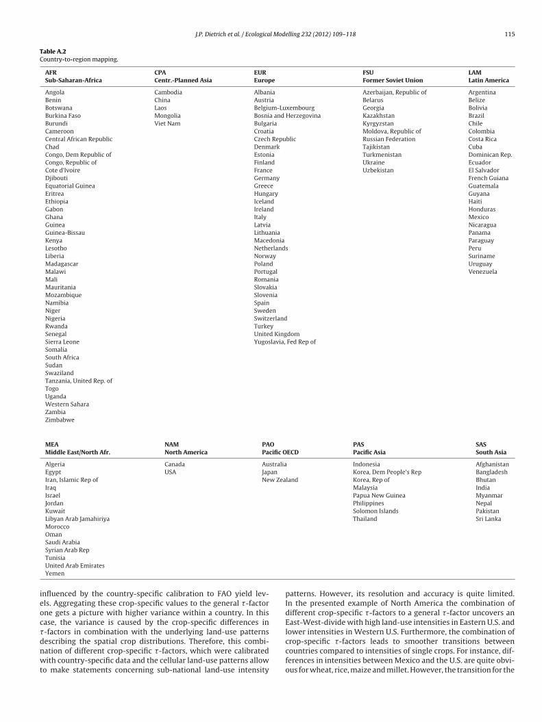

J.P. Dietrich et al. / Ecological Modelling 232 (2012) 109– 118 115

Table A.2Country-to-region mapping.

AFR CPA EUR FSU LAMSub-Saharan-Africa Centr.-Planned Asia Europe Former Soviet Union Latin America

Angola Cambodia Albania Azerbaijan, Republic of ArgentinaBenin China Austria Belarus BelizeBotswana Laos Belgium-Luxembourg Georgia BoliviaBurkina Faso Mongolia Bosnia and Herzegovina Kazakhstan BrazilBurundi Viet Nam Bulgaria Kyrgyzstan ChileCameroon Croatia Moldova, Republic of ColombiaCentral African Republic Czech Republic Russian Federation Costa RicaChad Denmark Tajikistan CubaCongo, Dem Republic of Estonia Turkmenistan Dominican Rep.Congo, Republic of Finland Ukraine EcuadorCote d’Ivoire France Uzbekistan El SalvadorDjibouti Germany French GuianaEquatorial Guinea Greece GuatemalaEritrea Hungary GuyanaEthiopia Iceland HaitiGabon Ireland HondurasGhana Italy MexicoGuinea Latvia NicaraguaGuinea-Bissau Lithuania PanamaKenya Macedonia ParaguayLesotho Netherlands PeruLiberia Norway SurinameMadagascar Poland UruguayMalawi Portugal VenezuelaMali RomaniaMauritania SlovakiaMozambique SloveniaNamibia SpainNiger SwedenNigeria SwitzerlandRwanda TurkeySenegal United KingdomSierra Leone Yugoslavia, Fed Rep ofSomaliaSouth AfricaSudanSwazilandTanzania, United Rep. ofTogoUgandaWestern SaharaZambiaZimbabwe

MEA NAM PAO PAS SASMiddle East/North Afr. North America Pacific OECD Pacific Asia South Asia

Algeria Canada Australia Indonesia AfghanistanEgypt USA Japan Korea, Dem People’s Rep BangladeshIran, Islamic Rep of New Zealand Korea, Rep of BhutanIraq Malaysia IndiaIsrael Papua New Guinea MyanmarJordan Philippines NepalKuwait Solomon Islands PakistanLibyan Arab Jamahiriya Thailand Sri LankaMoroccoOmanSaudi ArabiaSyrian Arab Rep

ieoc�dnwt

TunisiaUnited Arab EmiratesYemen

nfluenced by the country-specific calibration to FAO yield lev-ls. Aggregating these crop-specific values to the general �-factorne gets a picture with higher variance within a country. In thisase, the variance is caused by the crop-specific differences in-factors in combination with the underlying land-use patterns

escribing the spatial crop distributions. Therefore, this combi-ation of different crop-specific �-factors, which were calibratedith country-specific data and the cellular land-use patterns allow

o make statements concerning sub-national land-use intensity

patterns. However, its resolution and accuracy is quite limited.In the presented example of North America the combination ofdifferent crop-specific �-factors to a general �-factor uncovers anEast-West-divide with high land-use intensities in Eastern U.S. andlower intensities in Western U.S. Furthermore, the combination of

crop-specific �-factors leads to smoother transitions betweencountries compared to intensities of single crops. For instance, dif-ferences in intensities between Mexico and the U.S. are quite obvi-ous for wheat, rice, maize and millet. However, the transition for the

116 J.P. Dietrich et al. / Ecological Modelling 232 (2012) 109– 118

F ate. Th( l) sugac

gbC

Fy

ig. A.1. Crop-specific �-factors for North America (NAM) in 2000 and their aggregf) sugar beet, (g) cassava, (h) sunflower, (i) soybean, (j) groundnut, (k) rapeseed, (rop-types for each cell, is marked as (all).

eneralized land-use intensity is relatively smooth at the border ofoth countries. Same holds true for the border between the U.S. andanada.

ig. A.2. Schematic evolution of reference yield (ref), actual yield (act) and potentialield (pot) over time when technological change occurs but is not adopted.

e corresponding crop-types are: (a) wheat, (b) rice, (c) maize, (d) millet, (e) pulses,r cane. The aggregated �-factor, which is derived by calculating the mean over all

Appendix D. A methodological comparison of land-useintensity � and yield gap

Analysis of land-use intensity using � and yield gap analy-sis show methodologically some fundamental differences: whileyield gap analysis is measuring how much improvements are still

Fig. A.3. Schematic comparison of reference yield (ref), actual yield (act) and poten-tial yield (pot) on a wet and a dry location under the assumption that yields can onlybe increased by irrigation technologies.

J.P. Dietrich et al. / Ecological Modelling 232 (2012) 109– 118 117

bution

pbabwcm

s→Fas

D

itittual

guwa

di

D(

oawsfico

Fig. A.4. Global �-factor distri

ossible compared to the potential yield, a pre-defined upperound, the � factor is measuring how much improvements werepplied so far. If the total amount of possible improvements woulde time-independent and the same for any location, both measuresould always measure the same. However, this is typically not the

ase. The following examples show some situations in which theeasures will give different results.In the following it is assumed that the inverse of the yield gap

hould be used as a surrogate for land-use intensity (low yield gap high land use intensity, high yield gap → low land use intensity).

urthermore, reference yields in the given examples never exceedctual yields. This assumption is not relevant for the outcome butimplifies the shown schematics.

.1. Not adopted technological change (temporal behavior)

The first example illustrates differences in yield gap and land usentensity measures, when technological change takes place overime (e.g. newly bred varieties or improved production means) buts not being adopted (Fig. A.2). Assuming constant environmen-al conditions our measure for land use intensity � is unaffected:he actual yield (act) does not change as the production remainsnchanged as well as the environment remains stable. Accordingly,lso the reference yield (ref) does not change and � reports constantand use intensity.

The yield gap analysis on the contrary shows an increasing yieldap, as the potential yield increases but the actual yield remainsnchanged. Interpreted as land use intensity that would lead to therong conclusion that intensity decreases, even though production

nd production methods remain unchanged.The described behavior does not only exist in the temporal

omain. The following example shows a similar behavior occurringn the spatial domain.

.2. A world merely equipped with irrigation technologiesspatial behavior)

This example assumes a world with agricultural yields that cannly be improved by applying irrigation technologies. We compare

dry region (irrigation technologies have a major impact) with aet region (irrigation technologies have a marginal impact) in this

cenario (Fig. A.3). On the wet location, there is only a small dif-

erence between potential yield and actual yield as only marginalmprovements can be achieved with the available technologies,onsequently the yield gap is small. As possible improvementsn the location are low the difference between actual yield and

for the year 2000 for maize.

reference yield is also quite low, indicating low land use intensitymeasured with �.

On the dry location it is the other way around. Strong improve-ments are possible as irrigation technologies can significantlyimprove the yield: assuming that irrigation technologies are onlypartially applied there is still a significant yield gap (as there is still alot to improve) and the � factor is relatively high (as a lot has alreadybeen done). Using the � factor the wet location shows lower landuse intensities than the dry location as there is just no possibility tointensify yields on the wet location much. At the same time yieldgap analysis would report the higher intensity for the wet locationnot reflecting that the yields at the dry location are much strongeramplified due to intensification than on the wet location.

Yield gap analysis is a very powerful tool when it comes tocomparing the current productivity levels to what is currentlyachievable and it is a good counterpart to an analysis with � oranother intensity measure. However, when it comes to the anal-ysis of land use intensities in larger spatial or temporal domains(where potential yields are bound to change and very heteroge-neous environmental conditions have to be considered), the yieldgap analysis is less suitable than �.

Appendix E. Agricultural land-use intensity measured with� for maize

See Fig. A.4.

Appendix F. Supplementary Data

Supplementary data associated with this article can be found, inthe online version, at doi:10.1016/j.ecolmodel.2012.03.002.

References

Alston, J.M., Chan-Kang, C., Marra, M., Pardey, P., Wyatt, T., 2000. A Meta-Analysisof Rates of Return to Agricultural R&D: Ex pede Herculem? International FoodPolicy Research Institute (IFPRI), Research Report 113.

Alston, J.M., Norton, G., Pardey, P., 1995. Science Under Scarcity. Principles and Prac-tice for Agricultural Research Evaluation and Priority Setting. Cornell UniversityPress.

Biemans, H., Hutjes, R.W.A., Kabat, P., Strengers, B.J., Gerten, D., Rost, S., 2009. Effectsof precipitation uncertainty on discharge calculations for main river basins.Journal of Hydrometeorology 10, 1011–1025.

Bondeau, A., Smith, P., Zaehle, S.O.N., Schaphoff, S., Lucht, W., Cramer, W., Gerten,D., Lotze-Campen, H., Müller, C., Reichstein, M., 2007. Modelling the role of agri-culture for the 20th century global terrestrial carbon balance. Global Change

Biology 13, 679–706.

Boserup, E., Kaldor, N., 1977. The Conditions of Agricultural Growth: The Economicsof Agrarian Change under Population Pressure. Aldine De Gruyter.

Brookfield, H.C., 1993. Notes on the theory of land management. PLEC News andViews 1, 28–32.

1 l Mod

B

C

C

D

E

E

F

F

F

F

FG

G

I

J

K

L

L

18 J.P. Dietrich et al. / Ecologica

ruinsma, J., 2003. World Agriculture: Towards 2015/2030: An FAO Perspective.Earthscan/James & James.

oelli, T.J., Rao, D.S.P., 2005. Total factor productivity growth in agriculture: amalmquist index analysis of 93 countries, 1980–2000. Agricultural Economics32, 115–134.

ollatz, G.J., Ribas-Carbo, M., Berry, J.A., 1992. Coupled photosynthesis-stomatal con-ductance model for leaves of c4 plants. Australian Journal of Plant Physiology19, 519–538.

ietrich, J.P., 2011. Efficient Treatment of Cross-Scale Interactions in a Land-UseModel. Dissertation. Humboldt University, Berlin.

venson, R.E., Gollin, D., 2003. Assessing the impact of the green revolution, 1960 to2000. Science 300, 758–762.

wert, F., Rounsevell, M.D.A., Reginster, I., Metzger, M.J., Leemans, R., 2005. Futurescenarios of European agricultural land use: I. Estimating changes in crop pro-ductivity. Agriculture, Ecosystems & Environment 107, 101–116.

ader, M., Rost, S., Müller, C., Bondeau, A., Gerten, D., 2010. Virtual water content oftemperate cereals and maize: present and potential future patterns. Journal ofHydrology 384, 218–231.

AOSTAT, 2009. Food & Agriculture Organization of the United Nations StatisticsDivision. http://faostat.fao.org (accessed 11/6/2009).

äre, R., Grosskopf, S., Norris, M., Zhang, Z., 1994. Productivity growth, technicalprogress, and efficiency change in industrialized countries. The American Eco-nomic Review 84, 66–83.

arquhar, G.D., Caemmerer, S., Berry, J.A., 1980. A biochemical model of photosyn-thetic CO2 assimilation in leaves of c 3 species. Planta 149, 78–90.

ederico, G., 2005. Feeding the World. Princeton University Press.erten, D., Schaphoff, S., Haberlandt, U., Lucht, W., Sitch, S., 2004. Terrestrial vegeta-

tion and water balance-hydrological evaluation of a dynamic global vegetationmodel. Journal of Hydrology 286, 249–270.

osme, M., Suffert, F., Jeuffroy, M.H., 2009. Intensive versus low-input croppingsystems: what is the optimal partitioning of agricultural area in order toreduce pesticide use while maintaining productivity? Agricultural Systems 103,110–116.

ttersum, M.K.V., Rabbinge, R., 1997. Concepts in production ecology for analysis andquantification of agricultural input–output combinations. Field Crops Research52, 197–208.

ohnston, M., Licker, R., Foley, J., Holloway, T., Mueller, N.D., Barford, C., Kucharik, C.,2011. Closing the gap: global potential for increasing biofuel production throughagricultural intensification. Environmental Research Letters 6, 034028.

ates, R.W., Hyden, G., Turner, B.L., 1993. Population Growth and AgriculturalChange in Africa. University Press of Florida.

ambin, E.F., Meyfroidt, P., 2011. Global land use change, economic globalization,

and the looming land scarcity. Proceedings of the National Academy of Sciences108, 3465.

ambin, E.F., Rounsevell, M.D.A., Geist, H.J., 2000. Are agricultural land-use mod-els able to predict changes in land-use intensity? Agriculture, Ecosystems &Environment 82, 321–331.

elling 232 (2012) 109– 118

Licker, R., Johnston, M., Foley, J.A., Barford, C., Kucharik, C.J., Monfreda, C.,Ramankutty, N., 2010. Mind the gap: how do climate and agricultural manage-ment explain the ‘yield gap’ of croplands around the world? Global Ecology andBiogeography 19, 769–782.

Monfreda, C., Ramankutty, N., Foley, J.A., 2008. Farming the planet: 2. Geographic dis-tribution of crop areas, yields, physiological types, and net primary productionin the year 2000. Global Biogeochemical Cycles 22, 1–19.

Netting, R.M., 1993. Smallholders, Householders: Farm Families and the Ecology ofIntensive, Sustainable Agriculture. Stanford University Press.

Neumann, K., Verburg, P.H., Stehfest, E., Müller, C., 2010. The yield gap of global grainproduction: a spatial analysis. Agricultural Systems 103, 316–326.

Nin, A., Arndt, C., Hertel, T.W., Preckel, P.V., 2003. Bridging the gap between par-tial and total factor productivity measures using directional distance functions.American Journal of Agricultural Economics 85, 928–942.

Nishimizu, M., Page, J.M., 1982. Total factor productivity growth, technologicalprogress and technical efficiency change: dimensions of productivity changein Yugoslavia, 1965–78. The Economic Journal 92, 920–936.

OECD-FAO, 2009. Agricultural Outlook 2009-1018.Pingali, P., 2007. Westernization of Asian diets and the transformation of food sys-

tems: implications for research and policy. Food Policy 32, 281–298.Portmann, F., Siebert, S., Döll, P., 2010. Mirca2000 – global monthly irrigated

and rainfed crop areas around the year 2000: a new high-resolution data setfor agricultural and hydrological modeling. Global Biogeochemical Cycles 24,GB1011.

Rost, S., Gerten, D., Bondeau, A., Lucht, W., Rohwer, J., Schaphoff, S., 2008. Agriculturalgreen and blue water consumption and its influence on the global water system.Water Resources Research 44, 1–17.

Runge, C.F., Senauer, B., Pardey, P.G., Rosegrant, M.W., 2003. Ending Hunger in OurLifetime – Food Security and Globalization. The John Hopkins University Press.

Shriar, A.J., 2000. Agricultural intensity and its measurement in frontier regions.Agroforestry Systems 49, 301–318.

Sitch, S., Smith, B., Prentice, I.C., Arneth, A., Bondeau, A., Cramer, W., Kaplan, J.O.,Levis, S., Lucht, W., Sykes, M.T., et al., 2003. Evaluation of ecosystem dynam-ics, plant geography and terrestrial carbon cycling in the LPJ dynamic globalvegetation model. Global Change Biology 9, 161–185.

Turner, B.L., Doolittle, W.E., 1978. The concept and measure of agricultural intensity.The Professional Geographer 30, 297–301.

von Braun, J., 2007. The World Food Situation: New Driving Forces and RequiredActions. International Food Policy Research Institute, Food Policy Report.

Wagner, W., Scipal, K., Pathe, C., Gerten, D., Lucht, W., Rudolfs, B., 2003. Evaluation ofthe agreement between the first global remotely sensed soil moisture data withmodel and precipitation data. Journal of Geophysical Research D: Atmospheres

108, 9–15.

Waha, K., van Bussel, L.G.J., Müller, C., Bondeau, A., 2012. Climate-driven simulationof global crop sowing dates. Global Ecology and Biogeography 21, 247–259.

Willmott, C.J., 1982. Some comments on the evaluation of model performance. Bul-letin of the American Meteorological Society 63, 1309–1369.