measures of retirement benefit adequacy: which, why, for
TRANSCRIPT
Measures of Retirement Benefit Adequacy: Which, Why, for Whom, and How Much?
Sponsored by Society of Actuaries’ Pension Section and
Pension Section Research Committee
Prepared by Vickie Bajtelsmit Anna Rappaport LeAndra Foster
January 2013
©2013 Society of Actuaries, All Rights Reserved The opinions expressed and conclusions reached by the authors are their own and do not represent any official position or opinion of the Society of Actuaries or its members. The Society of Actuaries makes no representation or warranty to the accuracy of the information.

©2013 Society of Actuaries, All Rights Reserved Page 2
Executive Summary
This report focuses on measuring retirement benefit adequacy in light of both expected and unexpected expenses in retirement and linking the measurement to the needs and objectives of different stakeholder groups. The report begins with a conceptual discussion of benefit adequacy and the various ways it has been and can be measured. Adequacy measures examined include replacement ratios, projected expenditures, and minimum societal standards. Both income needs and lump sum equivalents are considered. Different measures are better suited to the needs of different stakeholders and at different life stages.
To investigate the impact of various risks on retiree welfare, we developed a simulation model of retirement spending, incorporating standard of living goals as well as investment, inflation, life, health, and long term care risks, with distributional assumptions for each random variable. This adds value to the existing literature in that it more realistically considers the combined impact of many of the risk factors faced by retirees. In addition to presenting the results of the base model, we also test several common retiree decisions that are expected to impact adequacy, including reducing the post-retirement standard of living, buying an annuity, buying long-term care insurance, delayed and early retirement, and the decision to pay off a home mortgage prior to retirement. The report concludes with ideas for future research, and recommendations and implications for each stakeholder group.
The key findings include the following.
• Many of the next generation of retirees are facing a big drop in their standard of living when they retire.
• The median American married couple at retirement earns approximately $60,000 a year and has approximately $100,000 in non-housing wealth (based on the 2010 Survey of Consumer Finances, adjusted for wage inflation and recent market performance).
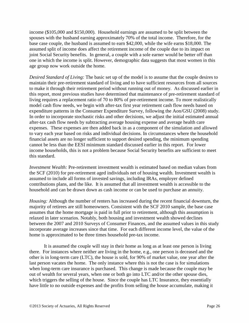
• The model shows there is a 29% chance median households will have positive wealth at death. The assets needed to meet cash flow needs 50 percent of the time would be approximately $170,000 compared to approximately $686,000 for a 95 percent success rate (See Table 10). Results are presented for two additional income levels and two wealth levels for each.
• There is no "one-size-fits-all" measure of benefit adequacy and there are many "moving parts" depending on the purpose and the stakeholder using it. Individuals need to be aware that attempts to over-simplify the retirement planning process can be very dangerous if used for personal decision making.
• The most appropriate measure of retirement benefit adequacy depends on the stakeholder: plan sponsor/employer; financial planner/individual; public policymaker; or financial institution.
• While it is much easier to plan for expected events, so-called "shock events" must be taken into consideration since they are more likely to derail an individual's retirement plan, especially at lower income levels. For the median income individual, shocks are the biggest driver of asset depletion.
©2013 Society of Actuaries, All Rights Reserved Page 3
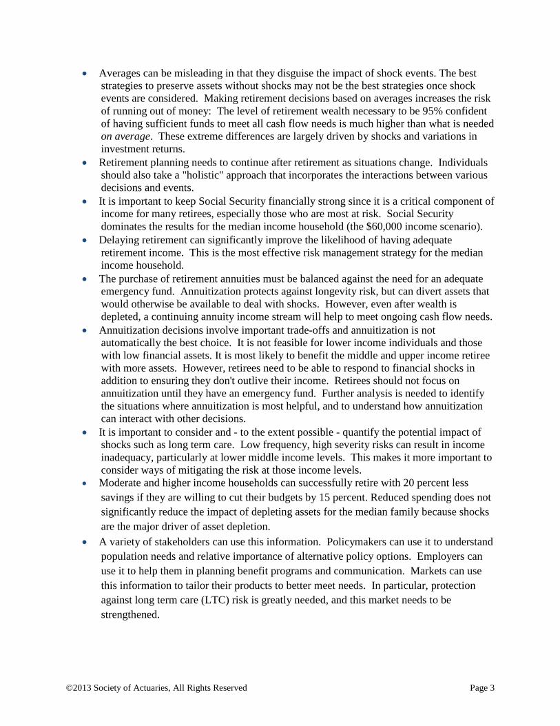
• Averages can be misleading in that they disguise the impact of shock events. The best strategies to preserve assets without shocks may not be the best strategies once shock events are considered. Making retirement decisions based on averages increases the risk of running out of money: The level of retirement wealth necessary to be 95% confident of having sufficient funds to meet all cash flow needs is much higher than what is needed on average. These extreme differences are largely driven by shocks and variations in investment returns.
• Retirement planning needs to continue after retirement as situations change. Individuals should also take a "holistic" approach that incorporates the interactions between various decisions and events.
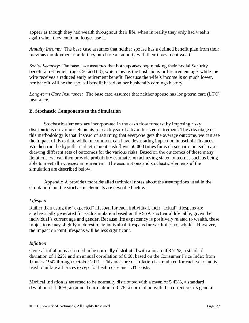
• It is important to keep Social Security financially strong since it is a critical component of income for many retirees, especially those who are most at risk. Social Security dominates the results for the median income household (the $60,000 income scenario).
• Delaying retirement can significantly improve the likelihood of having adequate retirement income. This is the most effective risk management strategy for the median income household.
• The purchase of retirement annuities must be balanced against the need for an adequate emergency fund. Annuitization protects against longevity risk, but can divert assets that would otherwise be available to deal with shocks. However, even after wealth is depleted, a continuing annuity income stream will help to meet ongoing cash flow needs.
• Annuitization decisions involve important trade-offs and annuitization is not automatically the best choice. It is not feasible for lower income individuals and those with low financial assets. It is most likely to benefit the middle and upper income retiree with more assets. However, retirees need to be able to respond to financial shocks in addition to ensuring they don't outlive their income. Retirees should not focus on annuitization until they have an emergency fund. Further analysis is needed to identify the situations where annuitization is most helpful, and to understand how annuitization can interact with other decisions.
• It is important to consider and - to the extent possible - quantify the potential impact of shocks such as long term care. Low frequency, high severity risks can result in income inadequacy, particularly at lower middle income levels. This makes it more important to consider ways of mitigating the risk at those income levels.
• Moderate and higher income households can successfully retire with 20 percent less savings if they are willing to cut their budgets by 15 percent. Reduced spending does not significantly reduce the impact of depleting assets for the median family because shocks are the major driver of asset depletion.
• A variety of stakeholders can use this information. Policymakers can use it to understand population needs and relative importance of alternative policy options. Employers can use it to help them in planning benefit programs and communication. Markets can use this information to tailor their products to better meet needs. In particular, protection against long term care (LTC) risk is greatly needed, and this market needs to be strengthened.
©2013 Society of Actuaries, All Rights Reserved Page 4
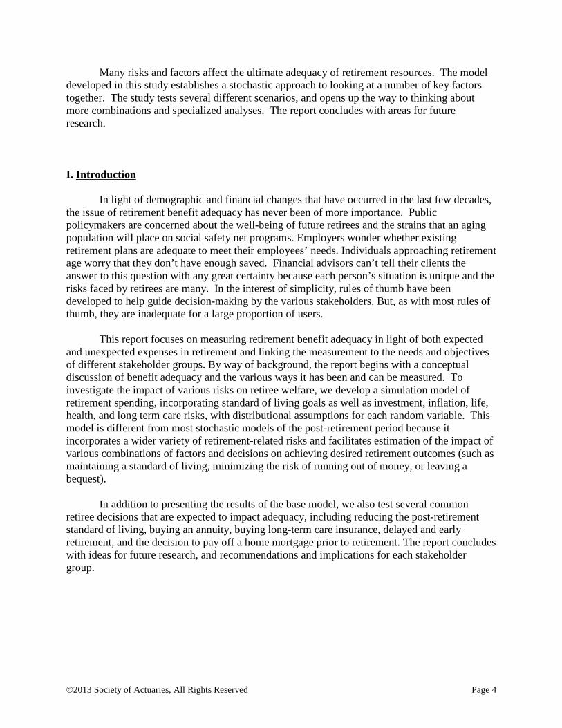
Many risks and factors affect the ultimate adequacy of retirement resources. The model developed in this study establishes a stochastic approach to looking at a number of key factors together. The study tests several different scenarios, and opens up the way to thinking about more combinations and specialized analyses. The report concludes with areas for future research.
I. Introduction In light of demographic and financial changes that have occurred in the last few decades, the issue of retirement benefit adequacy has never been of more importance. Public policymakers are concerned about the well-being of future retirees and the strains that an aging population will place on social safety net programs. Employers wonder whether existing retirement plans are adequate to meet their employees’ needs. Individuals approaching retirement age worry that they don’t have enough saved. Financial advisors can’t tell their clients the answer to this question with any great certainty because each person’s situation is unique and the risks faced by retirees are many. In the interest of simplicity, rules of thumb have been developed to help guide decision-making by the various stakeholders. But, as with most rules of thumb, they are inadequate for a large proportion of users. This report focuses on measuring retirement benefit adequacy in light of both expected and unexpected expenses in retirement and linking the measurement to the needs and objectives of different stakeholder groups. By way of background, the report begins with a conceptual discussion of benefit adequacy and the various ways it has been and can be measured. To investigate the impact of various risks on retiree welfare, we develop a simulation model of retirement spending, incorporating standard of living goals as well as investment, inflation, life, health, and long term care risks, with distributional assumptions for each random variable. This model is different from most stochastic models of the post-retirement period because it incorporates a wider variety of retirement-related risks and facilitates estimation of the impact of various combinations of factors and decisions on achieving desired retirement outcomes (such as maintaining a standard of living, minimizing the risk of running out of money, or leaving a bequest). In addition to presenting the results of the base model, we also test several common retiree decisions that are expected to impact adequacy, including reducing the post-retirement standard of living, buying an annuity, buying long-term care insurance, delayed and early retirement, and the decision to pay off a home mortgage prior to retirement. The report concludes with ideas for future research, and recommendations and implications for each stakeholder group.
©2013 Society of Actuaries, All Rights Reserved Page 5
II. Different Approaches to Adequacy and Related Background
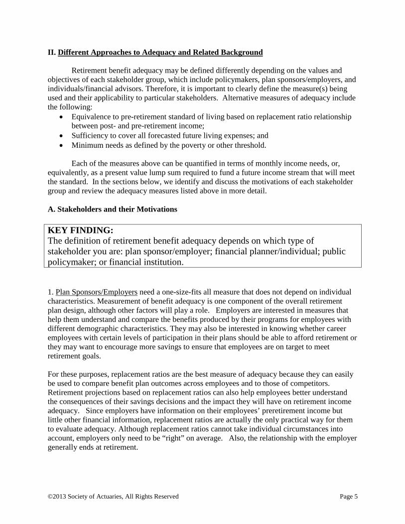
Retirement benefit adequacy may be defined differently depending on the values and objectives of each stakeholder group, which include policymakers, plan sponsors/employers, and individuals/financial advisors. Therefore, it is important to clearly define the measure(s) being used and their applicability to particular stakeholders. Alternative measures of adequacy include the following:
• Equivalence to pre-retirement standard of living based on replacement ratio relationship between post- and pre-retirement income;
• Sufficiency to cover all forecasted future living expenses; and • Minimum needs as defined by the poverty or other threshold.
Each of the measures above can be quantified in terms of monthly income needs, or,
equivalently, as a present value lump sum required to fund a future income stream that will meet the standard. In the sections below, we identify and discuss the motivations of each stakeholder group and review the adequacy measures listed above in more detail. A. Stakeholders and their Motivations KEY FINDING: The definition of retirement benefit adequacy depends on which type of stakeholder you are: plan sponsor/employer; financial planner/individual; public policymaker; or financial institution. 1. Plan Sponsors/Employers need a one-size-fits all measure that does not depend on individual characteristics. Measurement of benefit adequacy is one component of the overall retirement plan design, although other factors will play a role. Employers are interested in measures that help them understand and compare the benefits produced by their programs for employees with different demographic characteristics. They may also be interested in knowing whether career employees with certain levels of participation in their plans should be able to afford retirement or they may want to encourage more savings to ensure that employees are on target to meet retirement goals. For these purposes, replacement ratios are the best measure of adequacy because they can easily be used to compare benefit plan outcomes across employees and to those of competitors. Retirement projections based on replacement ratios can also help employees better understand the consequences of their savings decisions and the impact they will have on retirement income adequacy. Since employers have information on their employees’ preretirement income but little other financial information, replacement ratios are actually the only practical way for them to evaluate adequacy. Although replacement ratios cannot take individual circumstances into account, employers only need to be “right” on average. Also, the relationship with the employer generally ends at retirement.

©2013 Society of Actuaries, All Rights Reserved Page 6
2. Financial Planners/Individuals need an approach that can take personal preferences, needs, risks, and special circumstances into account. They need to produce a plan that will work for one person or family. The best approach for individuals is a detailed income needs forecast and conservative drawdown period plan that can be adjusted with changing circumstances. Planners also need to be able to explain the plan in order to justify monthly savings goals and lump sum targets for younger clients. CFP guidelines suggest that a detailed personal cash flow forecast is preferable to shortcut rules of thumb (See CFP-Board, 2012). However, such forecasts are relatively inaccurate until clients are approaching retirement age. For younger clients, it is relatively common for planners to make rough estimates based on replacement ratios. From the individual’s perspective (and that of their financial advisor), a successful retirement plan is one that allows them to meet retirement goals, one of which is likely to be financial self-sufficiency. Although individual goals may be quite different, they are nearly always quantifiable in terms of money costs, but will undoubtedly change over the retirement period. Thus, for a retirement plan to be successful, it is critical that the cash flow forecast incorporates expected changes over time, and not assume that the first year of retirement is representative of all years. The plan should also be revisited periodically and adjusted as needed. Unlike other stakeholder groups, individuals and their advisors need to be more concerned with downside risk. Whereas an employer is concerned with benefit adequacy on average, an individual who has insufficient income or assets in retirement bears the full consequences. Planners assess their clients’ sensitivity to downside risk in early interviews and will make more conservative recommendations for highly risk averse clients, so as to minimize the probability of investment losses and/or the overall risk of outliving wealth. 3. Policymakers have a variety of different concerns depending on the area of policy. They are most concerned with providing an appropriate safety net, reducing the risk of elderly poverty, and reducing reliance on Medicaid for long term care costs and health costs beyond Medicare. Policymakers are concerned with tax policy and want to be sure that the limits for tax-preferred employee benefits are appropriate. Policymakers are also concerned with the design and affordability of social benefits and the distribution of taxes for social benefits. It is desirable for them to understand how different policies drive behavior on the part of other stakeholders. As with plan sponsors/employers, this stakeholder group needs to be “right” on average, so a measure based on a population standard or on average income should meet the needs of policymakers. Policymakers should be interested in insights about how proposals relate to both minimum standards and desired post-retirement living standards. Policymakers should also be concerned about distributional effects and how policies affect retirees at different income levels. 4. In addition to these three main stakeholder groups, the financial services industry supports employers, plan sponsors, individuals, and financial advisors by developing products, services and software that meet the needs of each group. The industry is particularly interested in understanding needs and purchase behavior with regard to annuities, long term care insurance and supplemental medical insurance for older persons. Software organizations need to build tools that fit the needs of all stakeholders. The biggest challenges to software designers and individuals are addressing the needs of individuals and planners.
©2013 Society of Actuaries, All Rights Reserved Page 7
The model presented later in this report simulates future financial status and is related logically to a focus on replacement ratios, lump sums and a minimum needs standard. Using this model, we can test for adequacy of retirement resources under several different life paths and for different retirement strategies. In each case, we will need to measure outcomes against some accepted measure of adequacy. To that end, the next sections detail the background and conceptual framework for using replacement ratios, minimum needs standards, and detailed cash flow forecasts. B. Replacement Ratios Based on Preretirement Income The basic idea underlying replacement ratios is that one can define needs in retirement relative to income just before retirement, provided appropriate adjustments are made. This assumes that retirement income is intended to maintain a standard of living, in essence replacing a portion of a paycheck. For this to be an appropriate measure, it must be the case that most pre-retirement income was being spent. Therefore, replacement ratios may be less appropriate benchmarks for high-income households and/or those with greater than average savings rates. However, for low- to moderate-income households, paycheck replacement is an easily understood metric for focusing individuals on their needs after retirement. The traditional calculation of replacement ratios works best where earnings are relatively smooth and stable, and when it is practical to identify how expenses will change in retirement. For many years, employers with traditional pay scales and retirement plans used replacement ratios to understand what a career employee would get if they retired at age 65 after a full career with the organization, and to understand what they would get if they opted for earlier retirement. The adjustments from pre-retirement pay to a post-retirement equivalent would include removal of work related expenses, Social Security taxes, adjustments in other taxes, removal of assumed retirement savings, and adjustments for the difference in employee costs for health benefits. This worked best where the employer sponsored health benefits before and after retirement. Replacement ratios assume no significant change in lifestyle or major changes in expenses beyond those accounted for. Replacement ratio calculations can be based on gross income or after-tax income. Employer plans commonly used final pay or an average of pay for the last few years of earnings. Adjustments to pre-retirement income to define what should be replaced vary, as does the denominator used in different calculations. Because of these variations, it is critical that if replacement ratios are compared, they be calculated in a consistent manner and with consistent assumptions. Replacement ratios based on benefits from a specific plan require information about the plan provisions, earnings history, length of service, etc.

©2013 Society of Actuaries, All Rights Reserved Page 8
The Aon/Georgia State Study is a widely recognized study in the United States. The Aon (2008) study is the 7th study in a series that builds on a 1980 edition issued by the President’s Commission on Pension Policy.1
This study reflects common practice when plan sponsors use replacement ratios.
Aon (2008) recognizes four general changes from the pre- to the post-retirement period:
• Income taxes are reduced after retirement, because of the extra deduction for those over age 65 and because taxable income usually decreases at retirement.
• Social Security taxes end completely at retirement. (This of course assumes there is no
continued employment in retirement.)
• Social Security benefits are partially or fully tax-free. This reduces taxable income and the amount of income needed to pay taxes.
• Saving for retirement is no longer needed.
There is no adjustment for health care costs, as this is not a general issue, but one that must be handled on an employer or individual basis. For employers who offer pre-and post-retirement medical coverage, a general adjustment will provide insight with regard to their benefits.
For purposes of looking at Social Security benefits and the amount of income they replace, several definitions of replacement ratios are used. For example, Biggs and Springstead (2008) identify four alternative denominators for such measures:
• Final earnings • The constant income payable from the present value of lifetime earnings • The wage-indexed average of all earnings prior to claiming Social Security benefits • The inflation-adjusted average of all earnings prior to claiming Social Security benefits
using the Consumer Price Index for the calculation. For purposes of this paper, replacement ratios have been calculated using final pay as the denominator. The methodology used in the Aon/Georgia State work is generally similar to what is used for defining base case post-retirement spending in the model. The model description provides details on what is done in the calculations presented. For a discussion of the literature on replacement ratios and a detailed description of calculation
1 Aon Consulting’s Replacement Ratio Study, 2008. (Note that Aon Consulting subsequently merged with Hewitt Associates and is now part of Aon Hewitt.) This methodology is essentially continued in the AonHewitt study, The Real Deal, 2012. That study incorporates the updating of the Replacement Ratio study which will no longer be issued in the prior form.

©2013 Society of Actuaries, All Rights Reserved Page 9
of these ratios and of more variations, see MacDonald and Moore (2011). PRACTICAL ISSUE: Replacement ratios are best used for comparing participant results for large groups, as in the case of employer plans and social programs.
Replacement ratios are very useful for:
• Employer/plan sponsor who wants to understand what level of benefits will be delivered by its plan, or wants to compare the benefits from its plan with benefits from the plans of competitors. They are also useful in comparing plans when an employer is making changes to its program.
• Policymakers who want to understand what benefits are delivered by their plans or by social programs.
• Early career individuals who want some idea about whether their projected savings may be reasonably on target to enable them to replace current living standards.
• Rough estimate of retirement-readiness for individuals nearing retirement.
Replacement ratios are averages calculated based on a population and they focus at the time of retirement. They are not well suited to help those who are building a detailed plan for a household’s retirement because they fail to consider a number of individual issues and do not deal well with changes over time. They are also ill-suited to measure whether retirement resources will be adequate on an overall societal basis. PRACTICAL ISSUE: Replacement ratios make it difficult to incorporate individual differences and changes in expenses that occur during the retirement period.
Some of the limitations of using replacement ratios for personal retirement plans are:
• Families with children spend considerable money on child-rearing, particularly if the children go to college. Those are funds used during the years when the children are growing up and this spending may or may not continue in retirement depending on when the children become independent. When children graduate from college, there is often a big change in spending, which could be before retirement, at the time of retirement or later. In some situations, children return home later or need help during their parents’ retirement.

©2013 Society of Actuaries, All Rights Reserved Page 10
• For most families, housing is a major item of expense. Many households with mortgages try to pay them off before or close to time of retirement. In situations where mortgages are paid off, the out-of-pocket spending for housing is reduced significantly (and of course the amount of assets invested in financial investments is also reduced.) The modeling presented in this paper includes variations with regard to mortgage payoff.
• Other households choose to downsize their spending for housing by moving to a smaller house, or a less expensive area, or both. Replacement ratio calculations do not take mortgage status or downsizing of housing into account. They also do not take into account the purchase of a second home.
• Spending needs and priorities change over time. Inflation increases year by year
spending and health costs tend to rise with increasing age. Retirees may travel more in the early years of retirement, but less in later years.
• Before retirement, income changes over time, as do spending patterns. Income patterns can be smooth, but in many cases they are not.
• Debt over the life cycle can also be a major factor. Credit may be used to increase consumption during one period as compared to another, or to enable making major purchases and paying for them over time. Student loans commonly occur early in life, and repayment may reduce consumption for a period of years. Recent evidence suggests that repayment of borrowing to fund children’s or grandchildren’s education costs may continue into early retirement years. Notably, the 2012 Retirement Confidence Survey shows that among workers, 20% say debt is a major problem and 42% a minor problem. Among retirees, 12% say debt is a major problem and 25% a minor problem.
• Those retirees who choose to move into “senior housing” may find it costs more,
sometimes much more. Retirees with physical disabilities or cognitive limitations who wish to remain independent may find that they need help which may be quite costly.
• When pre-retirement earnings vary substantially, earnings near retirement age are not a good base from which to estimate required retirement income. The methodology also does not fit well for commissioned sales persons with significant earnings variations.
• This methodology does not translate well to phased retirement scenarios, such as those working in retirement or working part-time as they near retirement age
• One of the big decisions people need to make is when to retire, and they need to be able
to evaluate the impact of retiring at different times. The replacement ratio calculation is not well suited to helping evaluate differences in retirement timing. The overall assets needed for retirement are lower if one retires at a later age. Depending on how the replacement ratio is calculated, it may mask much of what is changing over time.
• Taxes should be considered, and need to reflect the individual’s personal tax situation.
©2013 Society of Actuaries, All Rights Reserved Page 11
• As individuals make decisions about retirement, they often have to choose between scaling down and working longer. Replacement ratios do not provide help in evaluating these trade-offs.
• Implicit in the methodology is long-term savings, generally at a constant rate. Some people do not save much for retirement in the early and middle years of working, but save heavily in the years near retirement. Traditional replacement ratios do not fit this pattern. Replacement ratios have been criticized repeatedly. The critics often recognize the
limitations, but may not focus on the fact that the limitations have different significance for different stakeholders, and they continue to have a place in the discussion of average retirement benefits by institutions and in the comparison of benefit delivery between plans.
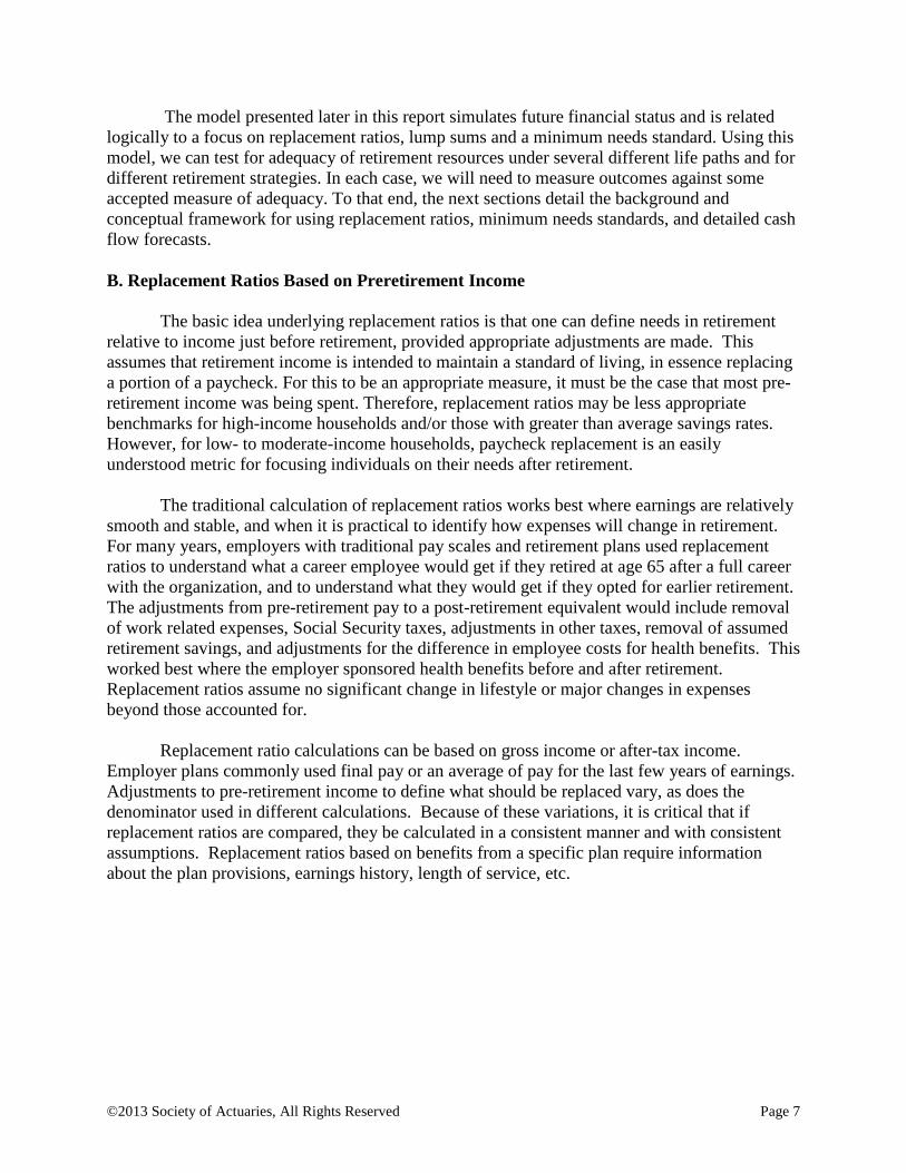
Table 1 below provides base case replacement ratios at age 65 needed to replace pre-retirement income from the Aon (2008) study. Table 1
Aon Baseline Replacement Ratios (married ages 65/62, one working) Pre-Retirement Income Replacement Ratios (2008 study)
From Social Security From Private and Employer Sources
Total Ratio
$ 20,000 69% 25% 94% $ 30,000 59% 31% 90% $ 40,000 54% 31% 85% $ 50,000 51% 30% 81% $ 60,000 46% 32% 78% $ 70,000 42% 35% 77% $ 80,000 39% 38% 77% $ 90,000 36% 42% 78%
$ 150,000 23% 61% 84% $ 200,000 17% 69% 86% $ 250,000 14% 74% 88% Source: Aon (2008), pp. 2, 12 Note that the income replacement from Social Security declines with increasing income,
and the amount needed from private sources increases with increasing income. The total ratio decreases until $80,000 of pre-retirement income and then increases at higher income levels due to higher employer-provided and individual retirement savings rates for those workers.

©2013 Society of Actuaries, All Rights Reserved Page 12
C. Minimum Needs Measures
A different approach is based not on maintaining preretirement standard of living, but on ensuring that resources are sufficient to meet some minimum level of needs. Wider Opportunities for Women (WOW), through its Elder Economic Security Initiative, is working with Brandeis University to establish a “minimum baseline” for what is required for an elder to live at a reasonable level (WOW, 2012).
The index includes a variety of monthly expenses and is developed for both couples and single persons and for renters as well as homeowners. In addition to national averages, indexes are developed separately at the community level in a number of states. Table 2 below summarizes key expense items and the Elder Index national average for several elder family types. Tables 3 and 4, adapted from information provided in WOW (2012), show how the Elder Index compares to other measures of income and to other measures of poverty, respectively.
Table 2: The Elder Economic Security Standard Index US Average Monthly Expenses for Selected Household Types, 2010
Elder Person Elder Person Elder Couple Elder Couple Monthly Expenses Owner w/o
Mortgage Renter Owner w/o
Mortgage Renter
Housing $372 $698 $372 $698 Food 231 231 424 424 Transportation (Private Auto)
283 283 346 346
Health care 254 254 508 508 Miscellaneous 228 228 330 330 Elder Index Per Month $1,368 $1,694 $1,979 $2,305 Elder Index Per Year $16,415 $20,328 $23,751 $27,773 Source: National Economic Security Initiative January 2012 Fact Sheet, citing Conahan, et al. (2006). Values inflated to 2010 using the Consumer Price Index. Table 3: Benchmarking Economic Security Against Common Sources of Retirement Income, 2010 Economic Security Index for a Single Elder Renter $20,328 Federal Poverty Level $10,380 Average Social Security Benefit -- Men $16,572 Average Social Security Benefit -- Women $12,526 Median Income in Retirement -- Men $19,985 Median Income in Retirement -- Women $15,775 Source: National Economic Security Initiative January 2012 Fact Sheet, citing Social Security Administration, Annual Statistical Supplement, 2009, Census Bureau, American Community Survey (2008), and Conahan, et al. (2006) Values inflated to 2010 using the Consumer Price Index and SSA COLAs.
©2013 Society of Actuaries, All Rights Reserved Page 13
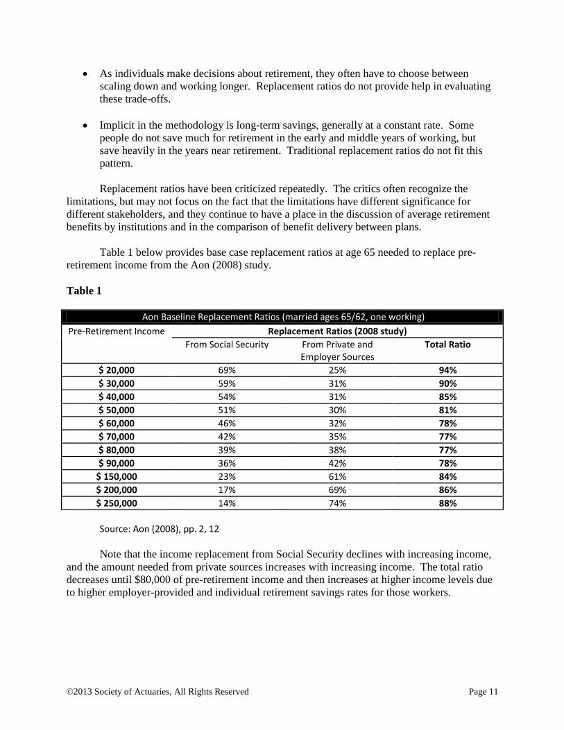
Table 4: Comparison of the 2010 WOW Elder Economic Security Index (Elder Index), the Official Poverty Threshold, and the Federal Supplemental Poverty Measure
Elder Index Official Federal
Poverty Index Supplemental Poverty Measure
Value for a 2 person family
$27,661 for 2 elder renters
$14,570 for two people
$15,939 for two renters
Adjusted for age Yes No No Adjusted for housing status
Yes No No
Adjusted for family size Yes Yes Yes Used for public assistance eligibility
No Yes No
Purpose Measures basic economic security including a variety of spending needs
Defines official poverty level
More sophisticated measure of poverty
Assumptions Assumes retirement, Medicare, car ownership Factors in food, housing, transportation, health care, and miscellaneous expenses
Assumes food is 1/3 of household budget
Factors in food, clothing, housing, utilities, health care, and taxes
Source: Adapted from fact sheet from Wider Opportunities for Women
The WOW Elder Index provides a much sounder measure of minimum retirement income needs than the poverty level. This is very helpful information for policymakers and, although not typically used, could provide a different perspective to employers/plan sponsors on the sufficiency of retirement plan benefits for long service employees. However, as with replacement ratios, these minimum standards are group averages that do not reflect individual needs and circumstances, or preferences.
Planners and individuals could also use minimum standards, such as the Elder Index, to establish a baseline. In that case, it would be best to use information for the local area. If an

©2013 Society of Actuaries, All Rights Reserved Page 14
individual’s spending is compared to the baseline, it would offer some indication about whether there is the potential for significant reductions in expenditures. Reducing spending is one of the ways that retirees often say they manage risk. Many individuals will have significant reductions in resources if they retire, and the index provides insight as to whether it is reasonable to plan significant reductions in spending. Housing is a major area of spending for many people, and there are very wide variations in housing cost depending on the type, size and location of housing. This is an area for cost reduction, but at the same time, a large number of people would prefer not to leave their homes. For seniors covered by Medicare, the choice of a Medicare Advantage plan, depending on what is available in the local area, is a potential way to reduce overall health care spending.
The Elder Index can also be used by individuals who are not yet near retirement age. If the Index is projected to retirement age and used as a benchmark to compare against current savings levels projected, it can provide incentive for additional savings. An individual whose savings level will not bring them up to the level of the Index at retirement gets a strong warning that more savings is needed. When this is considered together with a projection based on a replacement ratio, it provides a target range based on a minimum standard of living and current living standards. D. Cash Flow Analysis Forecast (with Inflation Adjuster)
The best method to determine income needs in retirement is a personalized cash flow
forecast. In fact, knowing how to prepare a retirement income needs analysis of this type is a component of the required body of knowledge for Certified Financial Planners. Estimation of retirement income needs requires a detailed budget forecast, which is beyond the ability of most individuals, particularly with a longer term forecast. However, many financial advisors have software packages that facilitate development of cash flow forecasts for their clients. This methodology allows for personalized treatment of choices in retirement, age, housing, part-time work, investments, travel, and other changes in retirement. It can also incorporate differences in family makeup, such as children who have not yet finished college, special needs family members, and financial support of other family members. Because planners tend to work with high wealth clients, planning software commonly focuses on wealth accumulation and may not accommodate annuities and other approaches for drawdown that may be more appropriate for the middle market. PRACTICAL ISSUE: Detailed budget forecasts can accommodate individual differences, but require an understanding of current spending and expected spending decisions, many complex assumptions, and need frequent updating. Such forecasts are not practical when one is far away from retirement.
There are a number of complexities with regard to budget forecasts including the
following:

©2013 Society of Actuaries, All Rights Reserved Page 15
• One of the hardest things to determine is how long one will live, and budgeting does not
solve that problem. If one plans for an average life span, which is common in financial planning software packages, that implies a 50% chance of failure. Solutions to that issue include buying guaranteed life income, and/or planning for greater longevity.
• While some expenses are routine and on-going such as food and much of housing costs, others are harder to predict such as home and auto repairs.
• Expenses increase each year with inflation. Average inflation rates are hard to predict, and may not be a good predictor of the impact on an individual household. The effect varies by household. Health care, food, energy and housing inflation impact individual households in different ways. Health care costs, including out-of-pocket expenses and Medicare Part B premiums, may increase more rapidly than inflation and be a big factor for some households.
• Even though a family may know it is quite likely that they will eventually need long term care, they don’t know when the need will arise, and to what extent they will need to buy care in the market versus getting help from family members. If a couple or individual chooses to later move into senior housing that includes some support services, such housing can be expensive and may lead to an increase in costs.
• Many retirees may have to help support dependent children, parents, or other family members and it is hard to predict when family issues will arise.
• Retirees have more time for travel and leisure activities and as one develops hobbies and lifestyle, there are often costs associated with these activities.
• Some retirees choose to become “snowbirds”, increasing housing costs. • Tax situations vary and taxes must be paid on withdrawal of most amounts from
conventional Individual Retirement Accounts and 401(k) plans. • Taxes can vary depending on when you claim Social Security, and how you adjust other
resource use. • It is not uncommon to experience changes in family status, such as divorce or widowhood,
during retirement. • Many retirees reduce spending later in life as they travel less and change their activities, but
it is hard to predict when people may be ready for that. PRACTICAL ISSUE: Cash flow forecasts commonly focus on the first year of retirement and thus do not incorporate health and long term care risks that occur later in the retirement period.
Detailed budgeting is useful only for individuals and planners, and it is most useful as people are nearing or in retirement. When people are far away from retirement age, they do not know what they will be spending as they near retirement, let alone what they will need in retirement.
Budgeting is only practical for those people who have a detailed idea about what they are
currently spending. If budgeting is used for the first year only or for the first few years, there are
©2013 Society of Actuaries, All Rights Reserved Page 16
similar challenges in developing long term plans as with replacement ratios. The plan must incorporate the length of the retirement period, inflation, shocks and expected health care needs.
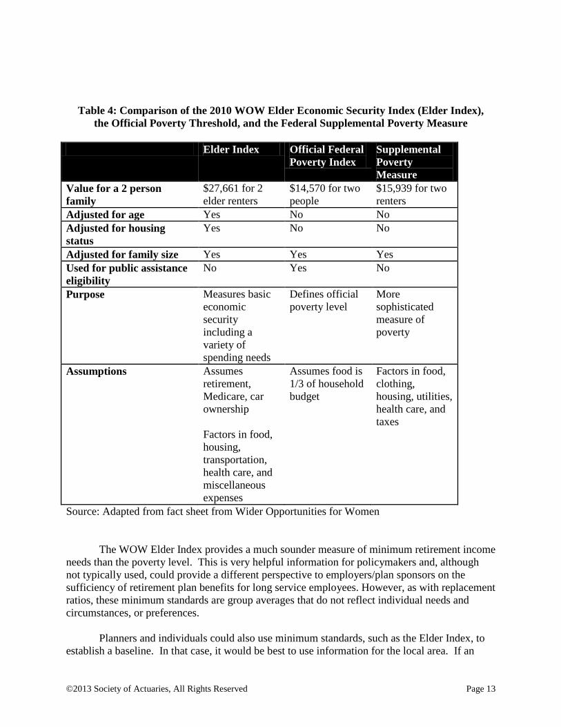
Data on average spending by age may also serve as a reference point for discussion and comparison. Table 5 shows 2009 spending by age for the civilian population excluding individuals residing in nursing homes, prisons, mental hospitals and other institutions. Average spending is considerably higher at ages 65-74 than for those over age 75, and the distribution of spending by category is also different. There are also more single person consumer units at ages 75 and over than at 65-74. Housing is by far the biggest category of spending in both age groups. Choices of where to live have a big impact on personal spending. People who live in higher cost areas, or in larger homes, can often reduce spending by moving to less expensive housing. However, this may be difficult if they own their homes and have to sell them. It should be noted that this data is per consumer unit and the Elder Economic Sufficiency Index provided earlier is for individuals and couples.
Table 5: Average Annual Expenditures per Consumer Unit Annual Amount Spent Percentage of Total Age 65-74 Age 75+ Age 65-74 Age 75+
Food & Alcohol $5,950 $4,377 13.9% 13.8% Housing $14,462 $11,811 33.7% 37.3% Apparel and Services $1,322 $793 3.1% 2.5% Transportation $7,033 $3,631 16.4% 11.5% Heath Care $4,906 $4,779 11.4% 15.1% Entertainment $2,498 $1,587 5.8% 5.0% Miscellaneous $2,030 $1,355 4.7% 4.3% Cash Contributions $2,087 $2,378 4.9% 7.5% Personal Insurance $2,669 $964 6.2% 3.0% Average Annual Total $42,957 $31,676 100.0% 100.0%
Source: Bureau of Labor Statistics, Consumer Expenditures Survey, 2009 E. Lump Sum Accumulation Target
The three measures of adequacy we have considered thus far (replacement ratios, minimum needs, and detailed forecast of cash flow needs) all focus on monthly or annual expenses in retirement. In practice, at younger ages, individuals and planners tend to focus more on a target amount of accumulated wealth. Of course, in many ways, the target wealth is simply another way of measuring the same thing, in that the wealth needed is the present value of the income that must be funded from savings, with some extra amount to cover the risk of the unexpected.
Focus on a lump sum presents some difficulties in that there are potentially multiple sources of income in retirement, some of which do not translate easily to lump sums. For example, social security benefits, benefits from employer defined benefit plans, and annuities are all income streams rather than lump sums. Therefore, the lump sum target needs to first take into account the proportion of income needs that will be met by expected income streams. If some of
©2013 Society of Actuaries, All Rights Reserved Page 17
these income streams are fixed and do not increase with inflation, the calculation of the lump sum target should take this into account as well. The remaining income needs can then be translated to a lump sum target. In practice however, most individuals do not understand the mathematics of present value, so are unlikely to be able to come up with the target wealth number on their own.
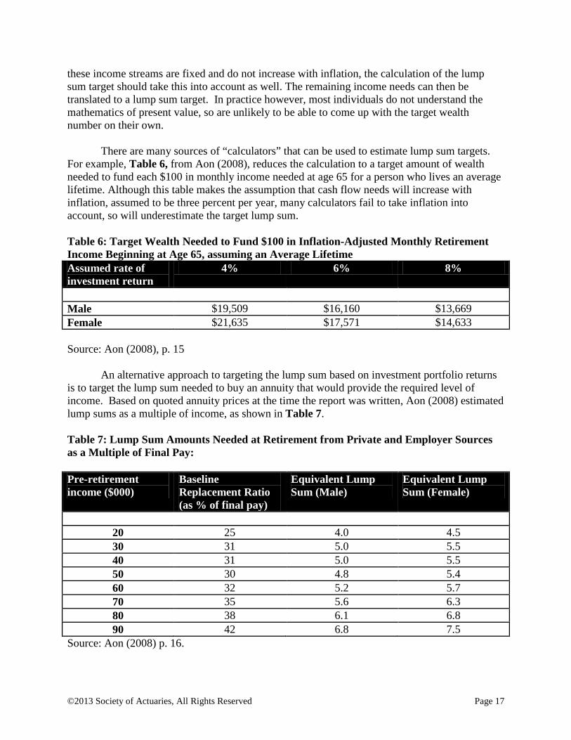
There are many sources of “calculators” that can be used to estimate lump sum targets. For example, Table 6, from Aon (2008), reduces the calculation to a target amount of wealth needed to fund each $100 in monthly income needed at age 65 for a person who lives an average lifetime. Although this table makes the assumption that cash flow needs will increase with inflation, assumed to be three percent per year, many calculators fail to take inflation into account, so will underestimate the target lump sum. Table 6: Target Wealth Needed to Fund $100 in Inflation-Adjusted Monthly Retirement Income Beginning at Age 65, assuming an Average Lifetime Assumed rate of investment return
4% 6% 8%
Male $19,509 $16,160 $13,669 Female $21,635 $17,571 $14,633 Source: Aon (2008), p. 15
An alternative approach to targeting the lump sum based on investment portfolio returns is to target the lump sum needed to buy an annuity that would provide the required level of income. Based on quoted annuity prices at the time the report was written, Aon (2008) estimated lump sums as a multiple of income, as shown in Table 7. Table 7: Lump Sum Amounts Needed at Retirement from Private and Employer Sources as a Multiple of Final Pay: Pre-retirement income ($000)
Baseline Replacement Ratio (as % of final pay)
Equivalent Lump Sum (Male)
Equivalent Lump Sum (Female)
20 25 4.0 4.5 30 31 5.0 5.5 40 31 5.0 5.5 50 30 4.8 5.4 60 32 5.2 5.7 70 35 5.6 6.3 80 38 6.1 6.8 90 42 6.8 7.5
Source: Aon (2008) p. 16.

©2013 Society of Actuaries, All Rights Reserved Page 18
The 2012 AonHewitt Real Deal study indicates that, at age 65, in addition to Social Security benefits, retirement resources equal to 11.0 times final pay are needed for their baseline case. Early retirees at age 62 would need 13.4 times pay and late retirees at age 67 would need 9.4 times pay. Without Social Security, total retirement resources needed would be 15.9 times final pay for the base case at age 65 That study also indicates that, on average, unsubsidized retiree health benefits account for about 30 percent of total resource needs (about 4.5 times final pay) but would be 5.1 times if the Affordable Care Act were not in place (AonHewitt, 2012, page 26). PRACTICAL ISSUE: Lump sum target estimates are highly sensitive to the lifespan, investment rate of return, and inflation assumptions. Practical issues in developing lump sums:
For most people, translating expected retirement needs into a total amount of retirement resources needed is challenging, even with software resources. A financial planner should be able to help. One of the advantages of using the services of a financial planner or advisor is that they can provide individualized estimates of both cash flow needs and lump sum retirement wealth targets. Although these can be developed individually, most large financial planning organizations have proprietary software that allows the planner to input key assumptions and provide their clients with the results of alternative scenarios (e.g. early retirement).
• Planners usually begin with some estimate of cash flow needs (either replacement ratio or detailed cash flow analysis), and subtract annuity streams (Social Security, defined benefit (DB) plans, and annuities) to determine additional retirement income needs that must be funded from invested assets. The income needs are then converted to a lump sum target based on assumed number of years in retirement and average investment returns.
• Results are highly sensitive to the choice of retirement period, investment rate of return and inflation rate.
• Planners usually base their estimates on expected mortality, although they have the ability to input longer lifespans to be more conservative.
• Software packages generally are not designed to incorporate phased retirement or health and long term care risks. Cash flow forecasts generally are for the first year of retirement. Financial advisors usually attempt to meet annually with each client to update their financial plans, although this is more likely to happen when the advisor is also the wealth manager and is responsible for investing on behalf of the client.
F. Withdrawal Rates and Drawdown of Retirement Savings
For a more complete review of the literature on drawdown of retirement savings, see MacDonald, et al. (2011). Perhaps due to its simplicity, there has been recent attention given to identifying “safe” withdrawal rates for retirement investment accounts. In this context, “safe” is usually defined in reference to a probability of ruin, or outliving one’s wealth. A common rule
©2013 Society of Actuaries, All Rights Reserved Page 19
of thumb that has been suggested and widely tested through simulation is the so-called “four percent rule” wherein it is recommended that if retirees withdraw four percent of their account balance in the first year of retirement and increase that withdrawal at the rate of inflation in future years, they have very low risk of outliving their portfolio. One way of thinking about this is that if your investment returns average four percent after inflation each year, the amount you have withdrawn will be made up for each year by investment earnings. However, the existence of market downturns means that you might have years in which your portfolio actually declines in value. Many papers have been appeared in the financial planning journals that purport to test or tweak the recommended withdrawal rates. Cooley, et al. compare different methodologies and conclude that a 4% withdrawal rate is sustainable for a 30 year retirement period, whereas Milevsky and Robinson (2005) peg it at 3.24%, with somewhat more conservative investment assumptions. Less favorable future investment returns or inflation, as compared to historical distributions, will tend to reduce the projected sustainable withdrawal rate. As with many rules of thumb, the primary advantage of focusing on a withdrawal rate is its simplicity. Although the decision requires assumptions about portfolio allocation, mortality, and investment return, the story appears to be “one size fits all” and is easy to explain to clients. The difficulty with this type of rule is that it is unrealistic. Unavoidable expenses, such as uninsured medical costs or auto repairs, may make it necessary to withdraw more than the safe amount. If the individual does so, it reduces the assets on which they earn investment returns and the forecasted safe withdrawal rate is no longer applicable. Most survey data indicates that very few retirees employ a systematic drawdown strategy, instead focusing on spending as needed. Similarly, very few people annuitize their retirement wealth, despite the advantages of transferring investment risk to an insurer.
PRACTICAL ISSUE: Simplified withdrawal rate rules are unrealistic in that they do not incorporate expense shocks such as auto and housing repairs, health and long term care costs. This study explicitly models health and long term shocks, and adjusts other expenses for inflation only. Annuities are a method of converting retirement wealth to an income stream and represent an alternative to do-it-yourself drawdown strategies. Nearly everyone has inflation-indexed guaranteed life income from Social Security and the amount of income can be increased by claiming benefits later. Some people have additional life income from employer-provided pensions but these are generally not adjusted for inflation. The amount of regular life income needed depends on individual circumstances and personal situations. For those who have sufficient assets to annuitize a portion of wealth, there are advantages and disadvantages. The potential impact of additional annuitization will be entirely different for those who live long than for those who die early. Individuals can outlive assets for several

©2013 Society of Actuaries, All Rights Reserved Page 20
reasons: living longer than expected; regular overspending; poor investment returns; and unexpected emergency expenditures or shocks. Annuitization provides a method of spreading out some part of assets over the individual’s remaining lifetime and transfers longevity and investment risk to the insurance company. Unless there is inflation protection, the real value of the payments declines with increases in the cost of living. The trade-off is that inflation-adjusted annuities will have smaller monthly payments at the start. Because monthly annuity payments are calculated assuming gradual “spend-down” of the asset and incorporate the pooling impact of those annuitants who die early, they are generally larger than what could alternatively have been safely withdrawn on one’s own. However, once an annuity is purchased, the decision is generally irrevocable, and unless the annuity includes refund on death or period certain features, there are no further death benefits after the last annuitant has died. Individuals commonly worry that, in the event of early death, they will not have gotten their “money’s worth” from an annuity purchase. This concern ignores the significant risk reduction they have received in return. Annuitization also offers some protection from cognitive decline and dementia, as the investment management and risk have transferred to an insurance company. Annuitization on a joint life basis protects both members of a couple, and protects the survivor after one has died. This is particularly important when the first-to-die spouse has experienced a prolonged illness that would have depleted household resources necessary for the survivor’s continued financial security. In the absence of annuitization, it is not uncommon for assets to be spent down when care is needed and the survivor is left with only Social Security and maybe their home. It also protects the other partner if one has a major need for long term care. Annuitization also discourages unplanned spending, but the individual can spend from other funds, or even borrow if they wish to spend more. Generally, annuitization is not a good idea unless there is an appropriate emergency fund in place. Annuitization also does not protect against shocks. An unmarried person who experiences a major long term care event, and who has annuitized a significant part of assets but not purchased long term care insurance may find that they are in a more difficult situation. Annuitization can take place at different times, or in steps. This study considers only a very simplified annuitization scenario in which the joint life annuity is purchased at retirement. Other alternatives that are not explored in this study include early or delayed purchase, and deferred annuities that do not begin payout until a later age, even as late as age 85.
III. Important Qualitative Issues
As individuals plan for their own retirement, there are many considerations and decisions that come into play. The Society of Actuaries has developed a series of 11 Decision Briefs (Society of Actuaries, 2012) for individuals nearing retirement to help them focus on the key decisions. Some of the decisions, risks and considerations are discussed below.

©2013 Society of Actuaries, All Rights Reserved Page 21
A. Part time work – traditional thinking about retirement was that people would work full-time in an established type of work until they retired all at once. In fact, many people change careers before they retire, and continue some type of work during retirement. (It is becoming increasing difficult to define a clear “date of retirement” and separate out retirees.) The 2012 Retirement Confidence study indicates that 70% of workers say they want to work in retirement but only 27% of retirees are working for pay in retirement (EBRI, 2012), Different terms have been used to refer to later in life careers, including encore careers and the third age. From a planning perspective, it is important to take expected work into account. At the same time, it is difficult to predict what will be feasible, and working in retirement is often more difficult to arrange than expected B. Retirement Age – for many middle-aged Americans, this is a critical decision with regard to well-being in retirement. For every year that retirement is delayed, funds are needed for one less year. Social Security monthly benefits are adjusted based on claiming age, and the monthly benefit is higher if one claims benefits later (within the 62 to 70 age range.) Spousal benefits are also impacted by claiming age. Other factors that change the balance between savings goals and resources are more time to save and earn investment income, increases in employer provided pensions, and fewer years without employer sponsored medical coverage. SOA research indicates that many Americans do not understand the impact on retirement well-being of retiring later, and that they underestimate the impact. They do understand the issues surrounding employer sponsored medical insurance (Society of Actuaries, 2011). Prior to the implementation of the Affordable Care Act, many families without employer sponsored retiree health have chosen to delay retirement to Medicare eligibility age. Others have paid a great deal for health insurance between the time of retirement and Medicare eligibility, particularly if they are in poor health, or have gone without coverage, hoping that they would not get seriously ill. However, those who want to retire later may not be able to do so. Both SOA research and the Retirement Confidence Study indicate that consistently over time people retire earlier than workers say they intend to, and that more than four out of ten workers retire earlier than planned (Society of Actuaries, 2011). One of the SOA Decision Briefs, “Big Question: When Should I Retire?” provides input on the considerations when making the decision about when to retire. C. Housing – housing is the largest item of spending for many households. Homeowners can reduce their out-of-pocket spending by paying off their mortgages. Middle American households approaching retirement age have about 70% of their assets in non-financial assets, primarily housing (Society of Actuaries Segmenting the Middle Market, 2010). Many of them plan to stay in their houses, but affordability can become an issue and there are other options. There is a huge variation in housing cost depending on the size of the home, location, etc. Renting out a room, and in some cases, moving in with family members, can also reduce housing cost. Housing equity can gradually be drawn down through the use of reverse mortgages, but this can be an expensive and somewhat risky strategy. There is special housing available for those who need help, which combines various levels of care with housing. The scenarios presented in this paper provide for home ownership with no mortgage at retirement, with five years, and with 10 years to payoff the mortgage. One of the SOA Decision Briefs “Where to Live in Retirement” discusses housing issues.
©2013 Society of Actuaries, All Rights Reserved Page 22
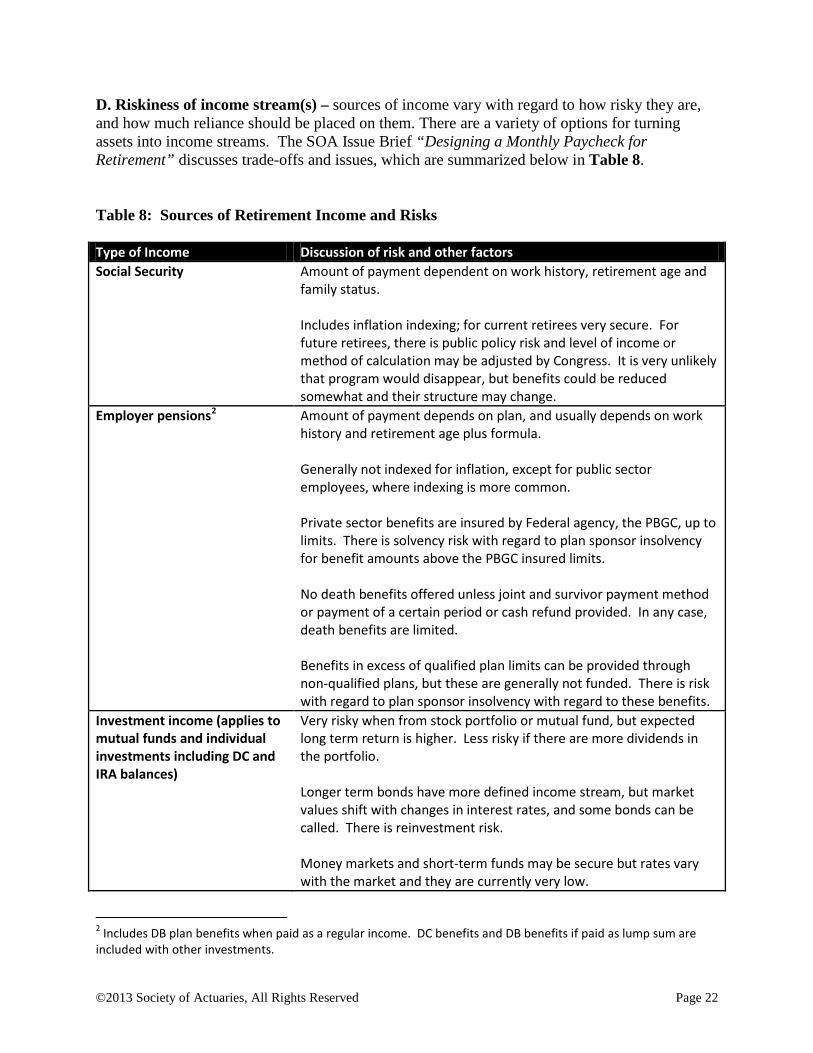
D. Riskiness of income stream(s) – sources of income vary with regard to how risky they are, and how much reliance should be placed on them. There are a variety of options for turning assets into income streams. The SOA Issue Brief “Designing a Monthly Paycheck for Retirement” discusses trade-offs and issues, which are summarized below in Table 8. Table 8: Sources of Retirement Income and Risks Type of Income Discussion of risk and other factors Social Security Amount of payment dependent on work history, retirement age and
family status. Includes inflation indexing; for current retirees very secure. For future retirees, there is public policy risk and level of income or method of calculation may be adjusted by Congress. It is very unlikely that program would disappear, but benefits could be reduced somewhat and their structure may change.
Employer pensions2 Amount of payment depends on plan, and usually depends on work history and retirement age plus formula.
Generally not indexed for inflation, except for public sector employees, where indexing is more common. Private sector benefits are insured by Federal agency, the PBGC, up to limits. There is solvency risk with regard to plan sponsor insolvency for benefit amounts above the PBGC insured limits. No death benefits offered unless joint and survivor payment method or payment of a certain period or cash refund provided. In any case, death benefits are limited. Benefits in excess of qualified plan limits can be provided through non-qualified plans, but these are generally not funded. There is risk with regard to plan sponsor insolvency with regard to these benefits.
Investment income (applies to mutual funds and individual investments including DC and IRA balances)
Very risky when from stock portfolio or mutual fund, but expected long term return is higher. Less risky if there are more dividends in the portfolio. Longer term bonds have more defined income stream, but market values shift with changes in interest rates, and some bonds can be called. There is reinvestment risk. Money markets and short-term funds may be secure but rates vary with the market and they are currently very low.
2 Includes DB plan benefits when paid as a regular income. DC benefits and DB benefits if paid as lump sum are included with other investments.
©2013 Society of Actuaries, All Rights Reserved Page 23
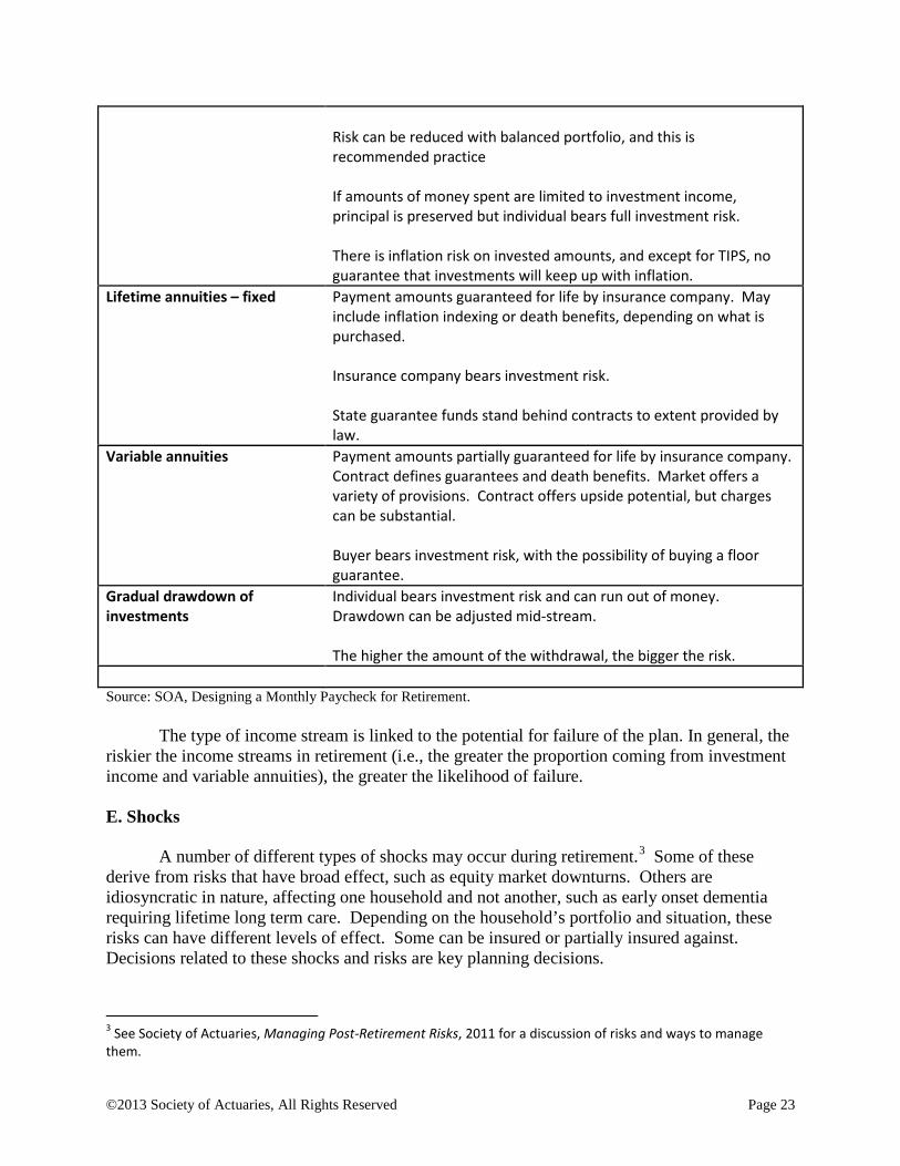
Risk can be reduced with balanced portfolio, and this is recommended practice If amounts of money spent are limited to investment income, principal is preserved but individual bears full investment risk. There is inflation risk on invested amounts, and except for TIPS, no guarantee that investments will keep up with inflation.
Lifetime annuities – fixed Payment amounts guaranteed for life by insurance company. May include inflation indexing or death benefits, depending on what is purchased. Insurance company bears investment risk. State guarantee funds stand behind contracts to extent provided by law.
Variable annuities Payment amounts partially guaranteed for life by insurance company. Contract defines guarantees and death benefits. Market offers a variety of provisions. Contract offers upside potential, but charges can be substantial. Buyer bears investment risk, with the possibility of buying a floor guarantee.
Gradual drawdown of investments
Individual bears investment risk and can run out of money. Drawdown can be adjusted mid-stream. The higher the amount of the withdrawal, the bigger the risk.
Source: SOA, Designing a Monthly Paycheck for Retirement.
The type of income stream is linked to the potential for failure of the plan. In general, the riskier the income streams in retirement (i.e., the greater the proportion coming from investment income and variable annuities), the greater the likelihood of failure. E. Shocks
A number of different types of shocks may occur during retirement.3
Some of these derive from risks that have broad effect, such as equity market downturns. Others are idiosyncratic in nature, affecting one household and not another, such as early onset dementia requiring lifetime long term care. Depending on the household’s portfolio and situation, these risks can have different levels of effect. Some can be insured or partially insured against. Decisions related to these shocks and risks are key planning decisions.
3 See Society of Actuaries, Managing Post-Retirement Risks, 2011 for a discussion of risks and ways to manage them.

©2013 Society of Actuaries, All Rights Reserved Page 24
PRACTICAL ISSUE: Retirement planning should consider the impact of shocks, such as:
• Major declines in financial asset values and/or returns • Major illness of self or spouse • Loss of spouse through death or divorce • Serious disability or dementia of self or spouse • Unusual longevity
Management strategies include avoidance, prevention, and risk transfer. There are usually trade-offs. For example, one can avoid stock market risk by using more conservative investments. The trade-off is lower expected investment return.
Asset allocation will drive the amount of market risk that the individual retirement plan is exposed to. There is a trade-off between expected long term return and the amount of risk borne.
One can plan for the loss of a spouse from a financial perspective through the use of survivor pensions, life insurance and maintaining assets that will remain with the spouse. One can plan for loss in other ways by thinking about the capability of the spouse and what is feasible for them if they are alone.
Health insurance provides protection for the financial consequences of major illness. Working to stay healthy reduces but does not eliminate the risk. Long term care insurance helps to offset the costs of care needed on major disability.
Where households decide to assume the risk, their response may occur after the event has occurred without much prior planning, or there may be plans in place. In some cases, people are well prepared for risks whereas in others they are completely unprepared. F. Risk Aversion
For households with financial assets and without defined benefit income in addition to Social Security, the issue of how much to drawdown assets and what can be spent is a huge issue. Some portion of assets should be set aside as an emergency fund, and then the issue of drawdown is very important.
The simulation results are reported in the next section to reflect differences in risk aversion. Less risk-averse individuals may be satisfied with a 50 percent chance of having an adequate level of retirement income to meet their needs. Although the 50th percentile will be adequate on average, it also means that half the time it will be inadequate to maintain the desired standard of living. Individuals who are very risk averse will be more interested in the 95th percentile simulation results which reflect the goal of being “right” nearly all of the time.

©2013 Society of Actuaries, All Rights Reserved Page 25
One of the reasons for reporting these two levels of confidence is that we are not making any assumptions about how individuals trade off risk and reward and our conclusions are probabilistic, based on the percentage of simulated outcomes. However, it is worth noting here that the behavioral economics literature suggests that individuals may treat losses differently than gains and therefore overweight the negative outcomes. This could be particularly important for the types of tail risks faced in retirement, which, when they occur simultaneously, can have serious financial consequences. Although not directly related to our study, Tomlinson ( 2012) finds that differences in loss aversion can significantly change optimal portfolio allocation. Applying his approach to our simulation would suggest that individuals would prefer to make decisions based on a fairly high level of confidence in order to reduce their risk of loss as much as possible. Thus, the amount of wealth necessary to be 95 percent sure is going to be substantially larger than most people would expect. The impact of tail risks on household finances is also sensitive to the model parameters for each of these risks.
Many of the personal decisions related to post-retirement risk involve trade-offs. Those who are more risk averse will choose to do more risk management, which improves their results in adverse scenarios, but often at a cost, which lowers expected asset values. This is also true for risk protection decisions such as the purchase of long term care insurance and annuities.
For those with more investable wealth, risk aversion also impacts investment strategies. The analysis of alternative investment strategies is beyond the scope of this study. IV. A Simulation Model of Retirement Cash Flow Needs To provide the basis for estimation of retirement income needs and adequacy, we develop a Monte Carlo simulation model of retirement cash flows that incorporates the common risks and uncertainties faced by retirees, including longevity, inflation, investment, health, and long-term care risks. By varying assumptions, we can compare outcomes based on decisions such as expense reduction, mortgage payoff, purchase of annuities and long-term care insurance, delayed and early retirement. In the following subsections, we describe and justify the base case assumptions, explain the metrics used for reporting the simulation output, and the alternative scenarios that are simulated.
A. The Base Case: Married Couple, Ages 66/63, $60,000 Income, $100,000 Non-Housing Wealth The basic model construct is a detailed cash flow forecast for a retired married couple from the date of retirement to the date of the death of both spouses, with Monte Carlo simulation of risks. The base case is constructed around median values for income, wealth, housing, health care costs, and long-term care for a married couple, with the husband age 66 and the wife, age 63. Income: The base case couple is assumed to have $60,000 in household pre-retirement pre-tax income which is approximately the median for their age group from the 2010 Survey of Consumer Finances. Throughout the model, where applicable, taxes are modeled according to 2012 tax rules. We also consider households at approximately the 75th and 90th percentiles of
©2013 Society of Actuaries, All Rights Reserved Page 26
income ($105,000 and $150,000). Household earnings are assumed to be split between the spouses with the husband earning approximately 70% of the total income. Therefore, for the base case couple, the husband is assumed to earn $42,000, while the wife earns $18,000. The assumed split of income does affect the retirement income of the couple due to its impact on joint Social Security benefits. In general, a couple with a sole earner would be better off than one in which the income is split. However, demographic data suggests that most women in this age group now work outside the home. Desired Standard of Living: The basic set up of the model is to assume that the couple desires to maintain their pre-retirement standard of living and to have sufficient resources from all sources to make it through their retirement period without running out of money. As discussed earlier in this report, most previous studies have determined that maintenance of pre-retirement standard of living requires a replacement ratio of 70 to 80% of pre-retirement income. To more realistically model cash flow needs, we begin with after-tax first year retirement cash flow needs based on expenditure patterns in the Consumer Expenditure Survey, following the Aon/GSU (2008) study. In order to incorporate stochastic risks and other decisions, we adjust the initial estimated annual after-tax cash flow needs by subtracting average housing expense and average health care expenses. These expenses are then added back in as a component of the simulation and allowed to vary each year based on risks and individual decisions. In circumstances where the household financial assets are no longer sufficient to support desired spending, the minimum spending cannot be less than the EESI minimum standard discussed earlier in this report. For lower income households, this is not a problem because Social Security benefits are sufficient to meet this standard. Investment Wealth: Pre-retirement investment wealth is estimated based on median values from the SCF (2010) for pre-retirement aged individuals net of housing wealth. Investment wealth is assumed to include all forms of invested savings, including IRAs, employer defined contributions plans, and the like. It is assumed that all investment wealth is accessible to the household and can be drawn down as cash income or can be used to purchase an annuity. Housing: Although the number of renters has increased during the recent financial downturn, the majority of retirees are still homeowners. Consistent with the SCF 2010 sample, the base case assumes that the home mortgage is paid in full prior to retirement, although this assumption is relaxed in later scenarios. Notably, both housing and investment wealth showed declines between the 2007 and 2010 Surveys of Consumer Finances, and the assumed values in this study incorporate average increases since that time. For each different income level, the value of the home is approximated to be three times household pre-tax income.
It is assumed the couple will stay in their home as long as at least one person is living there. For instances where neither are living in the home, e.g., one person is deceased and the other is in long-term care (LTC), the house is sold, for 90% of market value, one year after the last person vacates the home. The only instance where this is not the case is for simulations when long-term care insurance is purchased. This change is made because the couple may be out of wealth for several years, when one or both go into LTC and/or the other spouse dies, which triggers the selling of the house. Since the couple has LTC Insurance, they essentially have little to no outside expenses and the profits from selling the house accumulate, making it
©2013 Society of Actuaries, All Rights Reserved Page 27
appear as though they had wealth throughout their life, when in reality they only had wealth again when they could no longer use it. Annuity Income: The base case assumes that neither spouse has a defined benefit plan from their previous employment nor do they purchase an annuity with their investment wealth. Social Security: The base case assumes that both spouses begin taking their Social Security benefit at retirement (ages 66 and 63), which means the husband is full-retirement age, while the wife receives a reduced early retirement benefit. Because the wife’s income is so much lower, her benefit will be the spousal benefit based on her husband’s earnings history. Long-term Care Insurance: The base case assumes that neither spouse has long-term care (LTC) insurance. B. Stochastic Components to the Simulation
Stochastic elements are incorporated in the cash flow forecast by imposing risky distributions on various elements for each year of a hypothesized retirement. The advantage of this methodology is that, instead of assuming that everyone gets the average outcome, we can see the impact of risks that, while uncommon, can have devastating impact on household finances. We then run the hypothetical retirement cash flows 50,000 times for each scenario, in each case drawing different sets of outcomes for the various risks. Based on the outcomes of these many iterations, we can then provide probability estimates on achieving stated outcomes such as being able to meet all expenses in retirement. The assumptions and stochastic elements of the simulation are described below.
Appendix A provides more detailed technical notes about the assumptions used in the simulation, but the stochastic elements are described below:
Lifespan Rather than using the “expected” lifespan for each individual, their “actual” lifespans are stochastically generated for each simulation based on the SSA’s actuarial life table, given the individual’s current age and gender. Because life expectancy is positively related to wealth, these projections may slightly underestimate individual lifespans for wealthier households. However, the impact on joint lifespans will be less significant.
Inflation General inflation is assumed to be normally distributed with a mean of 3.71%, a standard deviation of 1.22% and an annual correlation of 0.60, based on the Consumer Price Index from January 1947 through October 2011. This measure of inflation is simulated for each year and is used to inflate all prices except for health care and LTC costs. Medical inflation is assumed to be normally distributed with a mean of 5.43%, a standard deviation of 1.06%, an annual correlation of 0.78, a correlation with the current year’s general

©2013 Society of Actuaries, All Rights Reserved Page 28
inflation of .73, and a correlation with last year’s general inflation of .77. This information is also from the Consumer Price Index, taking only Medical Care costs, from January 1947 through October 2011. Medical inflation is simulated for each year and is used to inflate the costs of health care and LTC.
Investment Returns Investment wealth is assumed to be allocated between stocks (50% large cap and 50% small cap) and long-term corporate bonds. The portfolio allocation is assumed to change each year following the rule of thumb, where the percent of equity investment is 100 minus current age (e.g. At age 66 the equity portion is 100-66 = 34%). Using Ibbotson data from 1947 through 2010, the large cap/small cap portfolio returned an average of 14.2% with a standard deviation of 15.2%, while bonds average 6.5% with a standard deviation of 9.3%. Historical correlation was not significantly different than 0, so no correlations were used for investment returns. Each year, investment return is simulated assuming a lognormal distribution and a portfolio allocation based on the age of the older spouse. Note: These investment returns reflect “long-term” historical averages and do not specifically focus on current economic conditions. Some experts believe that future asset market returns may be lower than historical averages, in which case, the results of the simulations with respect to wealth needed to support retirement needs should be viewed as a lower bound. Alternative investment risk and return scenarios could be tested as part of future research.
Annual Health Expenditures Health expenditures are stochastically determined for each year of retirement based on a lognormal distribution. In the first year, health care costs are simulated with a mean of $2,000, standard deviation of $2,000, a minimum of $1,560, which is approximately the cost of Medicare Part B premiums, and a maximum of $100,000 (an extremely rare event). In each year thereafter, the mean, standard deviation, minimum and maximum increase based on simulated medical inflation. No special provision has been made to recognize higher health care costs for individuals who do not yet receive Medicare and who do not have employer sponsored health benefits. In the base case, the wife will not qualify for Medicare for two more years.
Long-Term Care Long term care is determined in a two-step process. First, each year it is determined if the individual will go into long term care based on a Bernoulli distribution where the probability is determined by the person’s age and gender. Next, if the person goes into LTC, the length of stay is assumed to be either three months or remaining life. While this is overly simplified, there is little information about the length of stay and reason for discharge and such complication adds little to the overall information from the simulation. The premium is assumed at a rate that will provide relatively complete coverage (Tomlinson, 2011).

©2013 Society of Actuaries, All Rights Reserved Page 29
C. Summary of Simulated Scenarios
In addition to the base case simulations for three income levels at two wealth levels each, we run the simulation with several variations that may be risk-increasing or risk-mitigating. The simulated elements described above apply to all of the scenarios that will be presented in the results section. Variations from the base case are described below and summarized in Table 9. Table 9: Summary of Simulated Income, Wealth, and Planning Decision Scenarios
NON-HOUSING WEALTH AT RETIREMENT $100,000 $200,000 $250,000 $500,000 $500,000 $1,000,000
Maintain Pre- retirement
Maintain Pre-retirement
Maintain Pre-retirement
Maintain Pre-retirement
Maintain Pre-retirement
Maintain Pre-retirement
Reduce 15% Reduce 15% Reduce 15% Reduce 15% Reduce 15% Reduce 15%0% 0% 0% 0% 0% 0%25% 25% 25% 25% 25% 25%50% 50% 50% 50% 50% 50%0 years 0 years 0 years 0 years 0 years 0 years5 years 5 years 5 years 5 years 5 years 5 years10 years 10 years 10 years 10 years 10 years 10 years66/63 66/63 66/63 66/63 66/63 66/6370/67 70/67 70/67 70/67 70/67 70/6762/62 62/62 62/62 62/62 62/62 62/62None None None None None NoneBoth (62/59) Both (62/59) Both (62/59) Both (62/59) Both (62/59) Both (62/59)Female (59) Female (59) Female (59) Female (59) Female (59) Female (59)
PRE-RETIREMENT INCOME
Retirement Age
Purchase LTC Insurance
$60,000 $105,000 $150,000
Standard of Living
% of Wealth Annuitized at Retirement
Time Until Payoff of Mortgage
Standard of Living Alternative At low levels of wealth, it may not be feasible to maintain the pre-retirement standard of living. In this scenario we reduce average expenditures by 15 percent but assume the same risk distribution for health and LTC costs, which are presumably outside of the retiree’s control.
Annuitization Alternatives One method of guaranteeing lifetime income is to purchase an annuity. In this scenario, we assume that a fixed joint life annuity is purchased with half of the initial investment wealth, with annuity payments to begin in the first year of retirement, continuing, without cost of living increases, until the second spouse passes away. Because of the unusually low interest rate environment, current rates on annuities are not very attractive. For the simulations, we project annuity prices based on an interest rate of 3.80%. This is higher than those in effect today, resulting in a lower lump sum price, but lower than historical

©2013 Society of Actuaries, All Rights Reserved Page 30
averages. No reflection of current market prices is included and there is no reflection of the value of competitive markets in these assumptions. The annuity is assumed to be priced based on the youngest spouse’s expected life span (according to the SSA’s actuarial life table). Clearly, there are many variations of annuity products available in the market. The results of this simulation scenario are specific to the product and pricing assumptions. An area for further study would be to investigate the risk-mitigating effects of different product types, such as variable and fixed, inflation-indexed, and combination products that include long term care coverage, as well as variations on the timing (immediate versus deferred).
Housing Alternatives While the majority of current retirees have their mortgages paid off prior to retiring, this simulation shows the effect of mortgage payments continuing five and 10 years into retirement. To determine the annual mortgage payment, it is assumed to be a standard 30-year mortgage, with 6% interest, and an original loan amount of 1.6 times pre-retirement income, which accounts for the house being purchased earlier in the couple’s life when they were earning a lower salary.
Long-term Care Insurance Alternatives In the base case, the household did not buy LTC insurance. Two simulation alternatives are run to estimate the impact of long-term care insurance: 1) both spouses purchase LTC insurance at retirement and 2) the wife purchases LTC insurance at age 63.
Retirement Date Alternatives Delayed retirement scenarios assumes the husband and wife will work until age 70 and age 67, respectively. The pre-retirement and wealth assumptions do not change; in other words, they still retire with a total income of $60,000 ($105,000 and $150,000) and investment wealth of $100,000 ($250,000 and $500,000). Social Security rewards people who work longer by increasing benefits. In this instance, the husband will receive 132% of his benefit, while the wife will receive 108% of her benefit (being the greater of her earned benefit or 50% of her husband’s earned benefit). V. Results and Discussion
For each of the simulated scenarios discussed in this section, we present several metrics (success/failure) that help to evaluate benefit adequacy.
• Probability of having wealth left at death: This is the percentage of the simulation runs in which the last spouse to die has any investment wealth remaining. The difference from 100% is the risk of outliving your assets. E.g., if the probability of having wealth left at death is 29%, then 71% of the time you can expect to experience an income shortfall.
• Expected wealth at death: For each run of the simulation, we determine how much money is left in the investment portfolio when the last spouse dies. On the tables below,

©2013 Society of Actuaries, All Rights Reserved Page 31
we report the midpoint of all the ending wealth values (50th percentile or median) and also the 95th percentile, which essentially says there is only a 5 percent chance of having that much.
• Number of Years Income is Insufficient to Meet Needs: This can be thought of as the number of years in retirement in which the household experiences an income shortfall, i.e., they have insufficient funds to fully meet their needs. The 50th percentile tells you that half the time the household can expect to be short for that many years. Because they still may have other sources of funds, such as social security or annuity income, this does not represent a bankruptcy estimate, but rather an estimate of the number of years in which they will not be able to meet their goal of maintaining pre-retirement standard of living. The income amounts during the period of shortfall will differ depending on whether or not they have purchased an annuity. (Note scenarios that include defined benefit income have not been tested.)
• Retirement Wealth That Would Have Been Sufficient to Meet Needs: This is an estimate of the target lump sum wealth the couple would have needed to start with to cover all of their expenses. Again, the 50th percentile tells them, on average, what they would have needed, whereas the 95th percentile tells them what they would have needed to have only a 5% chance of running short.
A. Base Case Table 10 summarizes the base case simulated retirement outcomes for all six income/wealth combinations. The results show that the $60,000 couple with only $100,000 in investment wealth at retirement faces a high probability of having inadequate income to meet their needs. They have wealth left at death only 29% of the time, which implies a 71% chance of shortfall.
©2013 Society of Actuaries, All Rights Reserved Page 32
Table 10: Base Case: Married Couple Retiring at Ages 66(M) and 63(F)
NON-HOUSING WEALTH AT RETIREMENT $100,000 $200,000 $250,000 $500,000 $500,000 $1,000,000
Probability of Having Wealth Left at Death: 29% 81% 8% 68% 14% 82%
Remaining Wealth at Death:50% of the time, less than: $0 $361,743 $0 $444,966 $0 $1,467,65295% of the time, less than: $235,705 $1,527,216 $89,484 $2,437,392 $383,896 $6,036,391
Number of Years Income is Insufficient to Meet Needs:
50% of the time, less than: 5 years 0 years 11 years 0 years 10 years 0 years95% of the time, less than: 21 years 12 years 24 years 13 years 22 years 9 years
Retirement Wealth That Would Have Been Sufficient to Meet Needs:
50% of the time: $169,628 $169,972 $544,521 $547,644 $949,613 $950,31495% of the time: $686,264 $686,533 $1,011,390 $1,068,873 $1,491,116 $1,525,269
$60,000 $105,000 $150,000PRE-RETIREMENT INCOME
KEY FINDING: Making retirement decisions based on averages increases the risk of running out of money: The level of retirement wealth necessary to be 95% confident of having sufficient funds to meet all cash flow needs is much higher than what is needed on average. These extreme differences are largely driven by shocks and variations in investment returns.
The extreme differences between the 50th and 95th percentiles illustrate the problems associated with focusing on averages. Although, on average, they will have sufficient income to meet their needs, there is still at least a five percent risk that they will have a long period of shortfall (nine to 24 years, depending on wealth and income). Although not apparent on this table, extreme tail risks, such as early onset long-term care needs, investment declines (particularly in the early years of retirement), inflation risk, and unexpected health costs all contribute to the likelihood of retirement income inadequacy. Not surprisingly, higher wealth at retirement improves the odds of making it through retirement without financial difficulties. Notably, the level of retirement wealth necessary to meet cash flow needs on average is quite different from what it takes to be 95 percent sure of having enough. For example, the lowest income couple would need $169,628 in expendable non-housing wealth at the time of
©2013 Society of Actuaries, All Rights Reserved Page 33
retirement to be 50% confident of having enough. But in order to be 95% confident of not running short, they would need four times as much ($686,264). In contrast, the $105,000 and $150,000 income couples would need $544,521 and $949,613 respectively to meet their needs on average, but approximately $1 million and $1.5 million, respectively to be 95% confident of having enough. At higher income levels, the results may at first seem counterintuitive in that they show much higher wealth needed and lower probabilities of having wealth left at death. There are two reasons for this result. First, the target levels of retirement income increase with pre-retirement income. Second, Social Security replacement ratios are much lower for higher income households, as illustrated in Figure 1 below. Social Security replaces about 43% for the $60,000 couple, but only 35% for the $105,000 couple and 30% for the $150,000 couple. This implies that, even though both couples have proportionally similar investment wealth relative to pre-retirement income, the higher income couple must fund more of their retirement expenditures. KEY FINDING: At lower income levels, Social Security benefits are extremely important and significantly reduce the amount of investment wealth necessary to fully fund retirement income needs. Figure 1

©2013 Society of Actuaries, All Rights Reserved Page 34
Several factors can mitigate or exacerbate the risk of income inadequacy in retirement. In the next subsections, we report the simulation results for the various alternatives that were identified above. B. Effect of Reduced Discretionary Spending KEY FINDING: Moderate and higher income households can successfully retire with 20 percent less savings if they are willing to cut their discretionary budgets by 15 percent. Reduced spending does not significantly improve outcomes for the median family because shocks are the major driver of asset depletion. If a household has insufficient wealth to maintain their preretirement spending levels, taking steps to reduce expenses is a logical retirement strategy. Table 11 reports the results of the simulation assuming a 15 percent reduction in discretionary spending starting immediately at time of retirement. Perhaps surprisingly, this strategy does not significantly improve outcomes for the lowest income group, but has a substantial impact on the middle and higher income hypotheticals. For example, the probability of having wealth left at death goes from eight percent to 54% for the middle income couple and from 14% to 32% for the higher income couple. Similarly, although wealth needs do not change for the $60,000 couple, the other two couples need about 20 percent less at retirement to be 95% confident of not outliving their assets. These results are in part a function of the greater importance of Social Security at lower income levels, as discussed in the previous section. Perhaps more important is that the retirement risks at the root of income shortfalls are extreme in nature (health, long term care, investments) and cannot be offset by relatively small reductions in annual expenditures when the household has relatively small resources. However, the middle and higher income couples can benefit from this strategy when it is combined with other risk-mitigating choices.
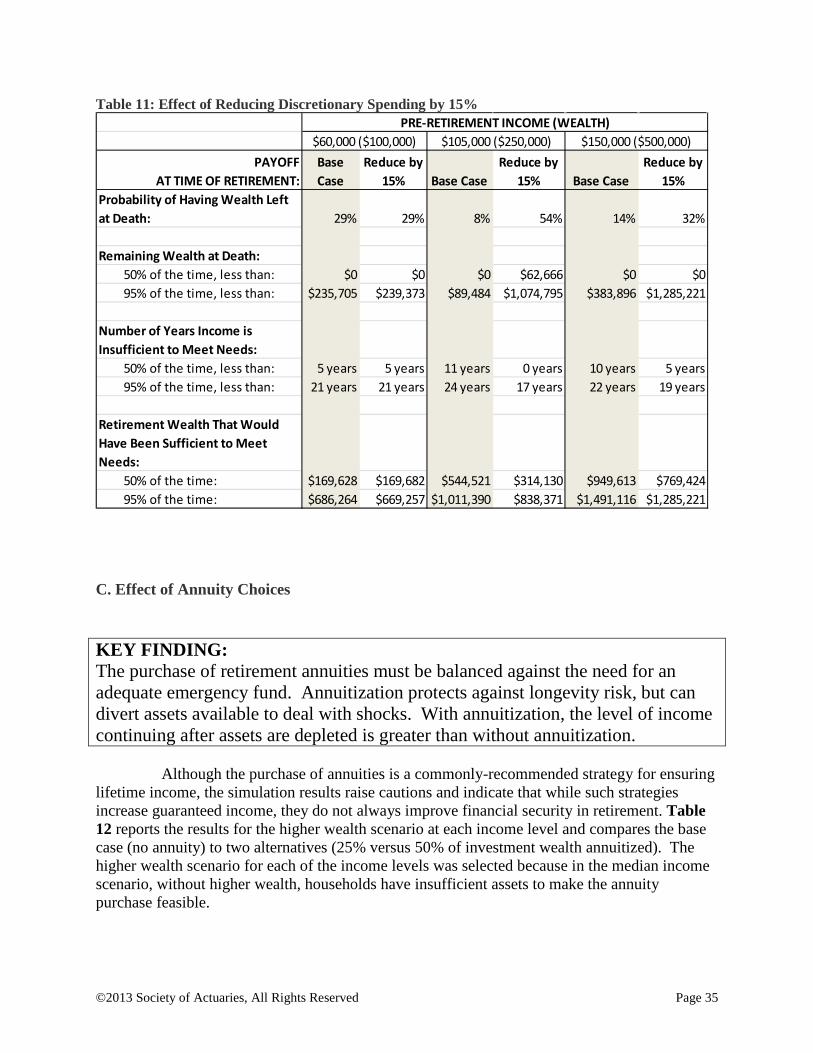
©2013 Society of Actuaries, All Rights Reserved Page 35
Table 11: Effect of Reducing Discretionary Spending by 15%
PAYOFF
AT TIME OF RETIREMENT: Base Case
Reduce by 15% Base Case
Reduce by 15% Base Case
Reduce by 15%
Probability of Having Wealth Left at Death: 29% 29% 8% 54% 14% 32%
Remaining Wealth at Death:50% of the time, less than: $0 $0 $0 $62,666 $0 $095% of the time, less than: $235,705 $239,373 $89,484 $1,074,795 $383,896 $1,285,221
Number of Years Income is Insufficient to Meet Needs:
50% of the time, less than: 5 years 5 years 11 years 0 years 10 years 5 years95% of the time, less than: 21 years 21 years 24 years 17 years 22 years 19 years
Retirement Wealth That Would Have Been Sufficient to Meet Needs:
50% of the time: $169,628 $169,682 $544,521 $314,130 $949,613 $769,42495% of the time: $686,264 $669,257 $1,011,390 $838,371 $1,491,116 $1,285,221
PRE-RETIREMENT INCOME (WEALTH)$60,000 ($100,000) $105,000 ($250,000) $150,000 ($500,000)
C. Effect of Annuity Choices KEY FINDING: The purchase of retirement annuities must be balanced against the need for an adequate emergency fund. Annuitization protects against longevity risk, but can divert assets available to deal with shocks. With annuitization, the level of income continuing after assets are depleted is greater than without annuitization. Although the purchase of annuities is a commonly-recommended strategy for ensuring lifetime income, the simulation results raise cautions and indicate that while such strategies increase guaranteed income, they do not always improve financial security in retirement. Table 12 reports the results for the higher wealth scenario at each income level and compares the base case (no annuity) to two alternatives (25% versus 50% of investment wealth annuitized). The higher wealth scenario for each of the income levels was selected because in the median income scenario, without higher wealth, households have insufficient assets to make the annuity purchase feasible.

©2013 Society of Actuaries, All Rights Reserved Page 36
PRACTICAL ISSUE: The simulation results reported here are sensitive to the assumptions about pricing of the annuity and timing of the purchase. Future research should address different products and factors, including the comparison of outcomes in situations where drawdown strategies typically fail, e.g., financial market downturns and unexpectedly long lives. Annuity purchase provides longevity protection and reduces income risk at later ages, but it comes at a cost. For all three income levels, the purchase of the annuities reduces the overall probability of having financial wealth at death and amount of wealth at death. This makes sense when you consider that the purchase of the annuity depletes resources available to meet unexpected expenses while increasing guaranteed life income. When the couple does not annuitize, running out of investment wealth leaves them only Social Security income. In contrast, a couple who has purchased an annuity and runs out of other investment wealth will have greater annual income than they would have otherwise. Although not modeled in this report, it is likely that the purchase of an annuity at a later age or the purchase of a deferred annuity would be a better financial strategy because it would more directly address longevity risk but at a lower upfront cost. More work is needed to better understand the situations where there is a significant benefit from annuitization and the types of annuity products that will best meet retiree needs The model assumes that investment returns are drawn from a long-run historical distribution whereas annuities are assumed to be priced based on more recent historical averages. In a low interest rate environment, annuity prices are not as attractive, which may have biased the results. Additional analysis on this issue was beyond the scope of this study, but is recommended for further work. Therefore, we do not feel that any strong conclusions can be made regarding the efficacy of annuitization strategies based on these results. Instead, we believe the main finding of importance with respect to annuities is the relative importance of maintaining an adequate emergency fund before diverting assets to the purchase of lifetime income products.
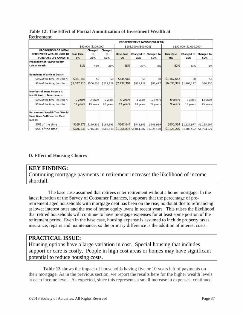
©2013 Society of Actuaries, All Rights Reserved Page 37
Table 12: The Effect of Partial Annuitization of Investment Wealth at Retirement
PROPORTION OF INITIAL RETIREMENT WEALTH USED TO
PURCHASE LIFE ANNUITY:Base Case
0%
Changed to
25%
Changed to
50%Base Case
0% Changed to
25%Changed to
50%Base Case
0% Changed to
25%Changed to
50%Probability of Having Wealth Left at Death: 81% 46% 29% 68% 37% 8% 82% 33% 6%
Remaining Wealth at Death:50% of the time, less than: $361,743 $0 $0 $444,966 $0 $0 $1,467,652 $0 $095% of the time, less than: $1,527,216 $500,655 $232,828 $2,437,392 $875,128 $81,427 $6,036,391 $1,409,287 $90,350
Number of Years Income is Insufficient to Meet Needs:
50% of the time, less than: 0 years 2 years 5 years 0 years 4 years 12 years 0 years 5 years 13 years95% of the time, less than: 12 years 19 years 20 years 13 years 18 years 24 years 9 years 19 years 25 years
Retirement Wealth That Would Have Been Sufficient to Meet Needs:
50% of the time: $169,972 $199,335 $169,993 $547,644 $548,165 $546,999 $950,314 $1,127,977 $1,125,69795% of the time: $686,533 $716,006 $689,510 $1,068,873 $1,044,307 $1,025,160 $1,525,269 $1,708,592 $1,704,622
PRE-RETIREMENT INCOME (WEALTH)$60,000 ($200,000) $105,000 ($500,000) $150,000 ($1,000,000)
D. Effect of Housing Choices KEY FINDING: Continuing mortgage payments in retirement increases the likelihood of income shortfall. The base case assumed that retirees enter retirement without a home mortgage. In the latest iteration of the Survey of Consumer Finances, it appears that the percentage of pre-retirement aged households with mortgage debt has been on the rise, no doubt due to refinancing at lower interest rates and the use of home equity loans in recent years. This raises the likelihood that retired households will continue to have mortgage expenses for at least some portion of the retirement period. Even in the base case, housing expense is assumed to include property taxes, insurance, repairs and maintenance, so the primary difference is the addition of interest costs. PRACTICAL ISSUE: Housing options have a large variation in cost. Special housing that includes support or care is costly. People in high cost areas or homes may have significant potential to reduce housing costs. Table 13 shows the impact of households having five or 10 years left of payments on their mortgage. As in the previous section, we report the results here for the higher wealth levels at each income level. As expected, since this represents a small increase in expenses, continued
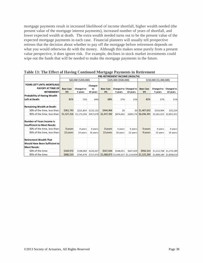
©2013 Society of Actuaries, All Rights Reserved Page 38
mortgage payments result in increased likelihood of income shortfall, higher wealth needed (the present value of the mortgage interest payments), increased number of years of shortfall, and lower expected wealth at death. The extra wealth needed turns out to be the present value of the expected mortgage payments in each case. Financial planners will usually tell prospective retirees that the decision about whether to pay off the mortgage before retirement depends on what you would otherwise do with the money. Although this makes sense purely from a present value perspective, it does ignore risk. For example, declines in stock market investments could wipe out the funds that will be needed to make the mortgage payments in the future. Table 13: The Effect of Having Continued Mortgage Payments in Retirement
YEARS LEFT UNTIL MORTGAGE PAYOFF AT TIME OF
RETIREMENT:Base Case
0% Changed to
5 years
Changed to
10 yearsBase Case
0% Changed to
5 yearsChanged to
10 yearsBase Case
0% Changed to
5 yearsChanged to
10 years
Probability of Having Wealth Left at Death: 81% 72% 64% 68% 37% 15% 82% 57% 51%
Remaining Wealth at Death:50% of the time, less than: $361,743 $221,854 $132,132 $444,966 $0 $0 $1,467,652 $316,904 $32,22495% of the time, less than: $1,527,216 $1,173,294 $957,678 $2,437,392 $874,662 $289,174 $6,036,391 $3,361,015 $2,852,351
Number of Years Income is Insufficient to Meet Needs:
50% of the time, less than: 0 years 0 years 0 years 0 years 4 years 9 years 0 years 0 years 0 years95% of the time, less than: 12 years 14 years 16 years 13 years 18 years 22 years 9 years 15 years 16 years
Retirement Wealth That Would Have Been Sufficient to Meet Needs:
50% of the time: $169,972 $198,969 $220,267 $547,644 $548,051 $647,429 $950,314 $1,212,708 $1,274,18995% of the time: $686,533 $745,479 $727,473 $1,068,873 $1,039,327 $1,114,659 $1,525,269 $1,808,184 $1,858,614
PRE-RETIREMENT INCOME (WEALTH)$60,000 ($200,000) $105,000 ($500,000) $150,000 ($1,000,000)

©2013 Society of Actuaries, All Rights Reserved Page 39
E. Effect of Long Term Care (LTC) Insurance KEY FINDING: The purchase of long term care insurance reduces emergency fund needs for lower income and wealth households.
As discussed previously, long term care is modeled as a low frequency, high severity risk. The probability is low, but the high cost can deplete household resources very quickly. As such, it results in a skewed distribution of outcomes that shows up in the wide discrepancies between the 50th and 95th percentile confidence levels. In the foregoing sections, we’ve seen that small increases in income or decreases in expenses do not mitigate the risk of income shortfall very effectively: this is because those strategies do little to improve household ability to meet long term care costs. To manage long term care risk and its impact on retiree household financial well-being, financial planners often recommend the purchase of long term care insurance. The impact of this purchase on our model is that households will have a small increase in regular expenses during retirement (premiums), but benefit from the lower expected cost of paying for care. If premiums were perfectly actuarially fair, these costs and benefits might be expected to offset each other, although risk averse individuals would probably prefer to pay the regular premium than to face the uncertainty of running out of money. Based on the results reported in Table 14, this strategy does have some risk-mitigating benefits, particularly for the lowest income couple. Based solely on the probability of having wealth remaining at death and the years without wealth, it appears that LTC insurance does more harm than good. However, when looking at the retirement wealth needed, the $60,000 couple needs half as much at retirement to be 95% confident of having enough. Due to the premium cost and the greater likelihood of survival, the purchase of LTC insurance for the wife only (as opposed to buying for both spouses) seems to have the greatest net benefit. For the higher income/wealth levels, LTC insurance is not as beneficial because they can afford to pay directly for the LTC and therefore do not need to incur the extra expense. A caveat to these results is that they are very sensitive to our assumptions about LTC risk and the type and timing of policy purchased. The results would be quite different if we assumed LTC insurance was purchased at younger ages or that the households purchased policies with less complete coverage at lower premiums. These results also do not consider product variations including combination products and those could be tested as an area for further research.
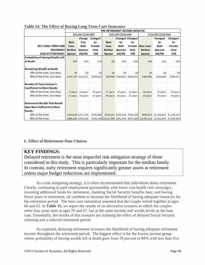
©2013 Society of Actuaries, All Rights Reserved Page 40
Table 14: The Effect of Buying Long Term Care Insurance
BUY LONG-TERM CARE INSURANCE
(AGE AT PURCHASE):
Base Case:
Neither Spouse
Changed to: Both
Spouses (62/59)
Changed to:
Female Only (59)
Base Case:
Neither Spouse
Changed to:
Both Spouses (62/59)
Changed to:
Female Only (59)
Base Case: Neither Spouse
Changed to:
Both Spouses (62/59)
Changed to:
Female Only (59)
Probability of Having Wealth Left at Death: 29% 10% 17% 8% 10% 10% 14% 11% 10%
Remaining Wealth at Death:50% of the time, less than: $0 $0 $0 $0 $0 $0 $0 $0 $095% of the time, less than: $235,705 $151,571 $168,327 $89,484 $206,812 $182,015 $383,896 $326,856 $298,317
Number of Years Income is Insufficient to Meet Needs:
50% of the time, less than: 5 years 14 years 10 years 11 years 15 years 13 years 10 years 15 years 14 years95% of the time, less than: 21 years 26 years 23 years 24 years 26 years 25 years 22 years 26 years 25 years
Retirement Wealth That Would Have Been Sufficient to Meet Needs:
50% of the time: $169,628 $227,193 $195,009 $544,521 $599,420 $581,169 $949,613 $1,166,852 $1,139,42795% of the time: $686,264 $333,218 $338,108 $1,011,390 $851,259 $871,180 $1,491,116 $1,623,874 $1,650,850
PRE-RETIREMENT INCOME (WEALTH)$60,000 ($100,000) $105,000 ($250,000) $150,000 ($500,000)
F. Effect of Retirement Date Choices KEY FINDINGS: Delayed retirement is the most impactful risk-mitigation strategy of those considered in this study. This is particularly important for the median family. In contrast, early retirement requires significantly greater assets at retirement unless major budget reductions are implemented.
As a risk mitigating strategy, it is often recommended that individuals delay retirement. Clearly, continuing in paid employment (presumably with lower cost health care coverage) , investing additional funds for retirement, claiming Social Security benefits later, and having fewer years in retirement, all combine to increase the likelihood of having adequate resources for the retirement period. The base case simulation assumed that the couple retired together at ages 66 and 63. In Table 15, we report the results of an alternative scenario in which the couples retire four years later at ages 70 and 67, but at the same income and wealth levels as the base case. Essentially, the results of this scenario are isolating the effect of delayed Social Security claiming and a reduced retirement period. As expected, delaying retirement increases the likelihood of having adequate retirement income throughout the retirement period. The biggest effect is for the lowest income group whose probability of having wealth left at death goes from 29 percent to 89% with less than five
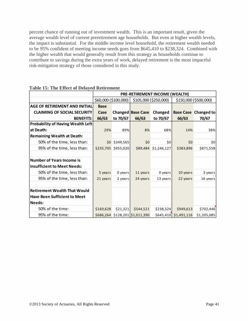
©2013 Society of Actuaries, All Rights Reserved Page 41
percent chance of running out of investment wealth. This is an important result, given the average wealth level of current preretirement age households. But even at higher wealth levels, the impact is substantial. For the middle income level household, the retirement wealth needed to be 95% confident of meeting income needs goes from $645,410 to $238,324. Combined with the higher wealth that would generally result from this strategy as households continue to contribute to savings during the extra years of work, delayed retirement is the most impactful risk-mitigation strategy of those considered in this study. Table 15: The Effect of Delayed Retirement
AGE OF RETIREMENT AND INITIAL CLAIMING OF SOCIAL SECURITY
BENEFITS:
Base Case 66/63
Changed to 70/67
Base Case 66/63
Changed to 70/67
Base Case 66/63
Changed to 70/67
Probability of Having Wealth Left at Death: 29% 89% 8% 68% 14% 38%Remaining Wealth at Death:
50% of the time, less than: $0 $349,565 $0 $0 $0 $095% of the time, less than: $235,705 $955,020 $89,484 $1,246,127 $383,896 $871,558
Number of Years Income is Insufficient to Meet Needs:
50% of the time, less than: 5 years 0 years 11 years 0 years 10 years 3 years95% of the time, less than: 21 years 2 years 24 years 13 years 22 years 16 years
Retirement Wealth That Would Have Been Sufficient to Meet Needs:
50% of the time: $169,628 $21,321 $544,521 $238,324 $949,613 $702,44695% of the time: $686,264 $128,201 $1,011,390 $645,410 $1,491,116 $1,205,085
$60,000 ($100,000) $105,000 ($250,000)PRE-RETIREMENT INCOME (WEALTH)
$150,000 ($500,000)

©2013 Society of Actuaries, All Rights Reserved Page 42
VI. Conclusions and Implications This study uses Monte Carlo simulation to simultaneously model stochastic investment, inflation, health, long term care, and life risks and evaluates several strategies for managing the risk of providing adequate retirement income to meet expenditure needs. More specifically, we consider which types of personal financial decisions best mitigate the risk of outliving retirement wealth.
The simulation results reported in the previous section allow us to draw several conclusions. First, and perhaps most importantly, both individuals and their advisors should be wary of relying on averages in estimating retirement resource adequacy. Particularly in the case of low frequency, high severity risks, such as long term care, average results will tend to disguise the extent of the potential shortfall risk faced by the individual. It is little comfort to know that you had sufficient funds on average if, in fact, you run out of money. Given that most individuals are risk averse, they should strive to make retirement and financial decisions that will result in retirement security most of the time rather than on average. Second, this report adds value by highlighting the risk-mitigating effects of several commonly recommended retirement strategies. In general, when considered in isolation, strategies focused on increasing income or decreasing expenses have only small marginal effects. While they do reduce the amount of wealth needed to fund cash flow needs on average, they have offsetting costs and do not mitigate the potentially large negative impact of expensive health and LTC shocks or ill-timed financial market downturns. Most risk management products today are single risk products, although there are some combination products in the market. The majority of middle market individuals could not afford to buy products to protect against all of the risks on a single risk basis. (Wealthy people could afford to buy these products but they can also self-insure.) Annuitization needs to be considered carefully and is not suitable in all situations. There is a trade-off between increasing guaranteed lifetime income and reducing the funds available to meet various risks and shocks. For those with relatively small assets, leaving assets in an emergency fund is often a better choice than annuitization because the reduction in emergency funds necessary to produce a fairly small incremental increase in income may not result in sufficiently better adequacy outcomes. The improvement in results from buying annuities is particularly important for those who live longer. Further analysis is needed to understand these implications. Annuitization is more likely to be desirable where there are enough assets to meet emergency fund needs, and to build a mixed portfolio that includes more lifetime income. Similarly, households retiring with remaining mortgage debt will have slightly larger expenses than those without, and will therefore need additional resources to cover the present value of the mortgage interest. As expected, early retirement, all else being equal, results in higher probability of income shortfall. Delayed retirement improves outcomes. Working longer is important for individuals

©2013 Society of Actuaries, All Rights Reserved Page 43
for increasing retirement security. Working part-time in retirement or phasing into retirement are also valuable strategies although not addressed in this report. Individuals should work to keep skills up-to-date so that they can work longer and they should save more earlier. For people with modest resources, the risk of paying for long term care is potentially the largest and earliest disruptor of retirement plans. For those people who require extended long term care, this can be a major shock to household financial resources. Although long term care services are often provided by family and friends, this study only considers the financial impact of entering a full-care facility, both with and without having purchased long-term care. Future research could incorporate the income and savings effects of providing long term care to family members. We also do not consider the availability of Medicaid as a last resort for LTC payment when assets have been exhausted. This coverage varies by state and facility, and is likely to be cut back in the future as states attempt to close their budget gaps. Given the extreme financial consequences of unplanned-for long-term care expenses, financial advisors are recommended to inform their clients about the availability and coverage options for long term care insurance. The results of our analysis suggest that for lower and moderate income families, the purchase of LTC insurance does indeed reduce the risk of running out of money and the amount of wealth required to be 95% confident of having enough. Offsetting those benefits is the slightly lower expected wealth at death, representing the future value of the additional expenditures for insurance premiums. In contrast, higher income families have enough wealth such that LTC costs do not play a substantial role in determining adequacy. A caveat to the results of this study is that each of the scenarios focuses on one issue at a time and therefore we cannot provide any insight on the efficacy of combinations of risk-mitigating strategies or products. We also consider only three income and wealth hypotheticals and do not explore how results might differ for those with particular characteristics, such as individuals who survive to later ages and those who experience financial hardship earlier in their retirement period. The issues discussed here point to the need for further research and exploration. A major implication and concern for all stakeholders is that many individuals are reaching traditional retirement ages without adequate retirement savings. Social Security remains extremely important to middle and lower income Americans and it is very important to keep it financially sound. The level of support for retirement offered by employers varies widely by company. Employers, particularly those with lower benefits, should think through whether their current benefit plans will create human resource challenges and problems in the future. Based on the median income and wealth values found in large national studies, we expect that households will need to take a combination of risk-mitigating steps, such as increasing savings, working longer, reducing expenses, developing plans for income in retirement, buying long term care insurance, and paying off mortgages. If steps are not taken, households face significant risk of depleting assets prior to death.
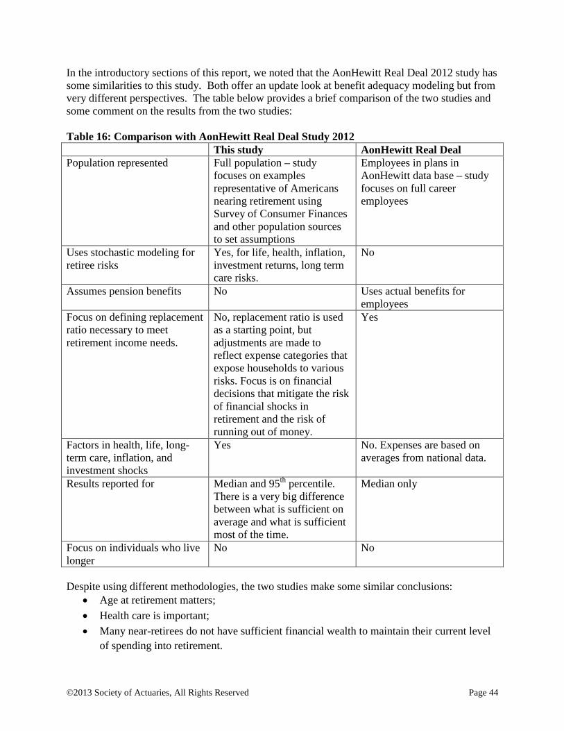
©2013 Society of Actuaries, All Rights Reserved Page 44
In the introductory sections of this report, we noted that the AonHewitt Real Deal 2012 study has some similarities to this study. Both offer an update look at benefit adequacy modeling but from very different perspectives. The table below provides a brief comparison of the two studies and some comment on the results from the two studies: Table 16: Comparison with AonHewitt Real Deal Study 2012 This study AonHewitt Real Deal Population represented Full population – study
focuses on examples representative of Americans nearing retirement using Survey of Consumer Finances and other population sources to set assumptions
Employees in plans in AonHewitt data base – study focuses on full career employees
Uses stochastic modeling for retiree risks
Yes, for life, health, inflation, investment returns, long term care risks.
No
Assumes pension benefits No Uses actual benefits for employees
Focus on defining replacement ratio necessary to meet retirement income needs.
No, replacement ratio is used as a starting point, but adjustments are made to reflect expense categories that expose households to various risks. Focus is on financial decisions that mitigate the risk of financial shocks in retirement and the risk of running out of money.
Yes
Factors in health, life, long-term care, inflation, and investment shocks
Yes No. Expenses are based on averages from national data.
Results reported for Median and 95th percentile. There is a very big difference between what is sufficient on average and what is sufficient most of the time.
Median only
Focus on individuals who live longer
No No
Despite using different methodologies, the two studies make some similar conclusions:
• Age at retirement matters; • Health care is important; • Many near-retirees do not have sufficient financial wealth to maintain their current level
of spending into retirement.

©2013 Society of Actuaries, All Rights Reserved Page 45
Policymakers can respond to the challenges in several ways:
• Enact policies that will support longer employment, and encourage employers to retain older workers.
• Do nothing and either ignore people who get into major trouble or address their needs
somewhat through social safety net programs.
• Encourage employers to offer more adequate benefits.
• Provide more incentives for retirement saving and at the same time make sure the money is not spent too early.
• Make it easier for employers to offer advice and products for the post-retirement period. Employers are concerned about fiduciary liability.
• Encourage new and more innovative financial products.
• Make it easier to offer products that combine long term care financing with other risk protection.
• Encourage efficient delivery methods to expand access to risk protection for middle income individuals.
• Strengthen Social Security and Medicare.
© 2013 Society of Actuaries, All Rights Reserved Page 46
VII. Future Research
This study provides a new approach for studying retirement income adequacy by simultaneously modeling stochastic investment, inflation, health, long term care, and life risks. While stochastic modeling is widely accepted in this area, other studies have primarily modeled investment returns, and have made assumptions based on averages for other types of risks faced by retirees. The advantage of our methodology over other studies is it allows us to study the interactions of retirement-related risks and the efficacy of strategies for managing those risks. Although the simulation results reported in this study provide many interesting findings, there are additional questions which deserve further investigation. Each of these areas could be the subject of a specialized study. Some of these possibilities are outlined below. Variations on Timing of Retirement and Phased Retirement In this study we considered only two variations on the timing of retirement and did not consider phased retirement. Many variations on the scenarios could be tested. Working in retirement and variations in retirement age as well as Social Security claiming age are huge issues with regard to retirement security. For families and individuals without very much retirement savings, they represent the areas where there is the greatest potential to make a difference in the longer term. There has been considerable work showing that claiming Social Security later is advantageous. One option occasionally discussed is using assets to provide more income in the early years of retirement while claiming Social Security later (in essence buying an inflation indexed annuity). This would be an area for a very fruitful further study. More In-depth Exploration of Long Term Care Risks and Financing Alternatives In this study, we model long term care using a rough distributional assumption on timing and costs. The results show that long term care is a major factor affecting the outcome for different families and the purchase of long term care insurance can have beneficial effects. In part because data is sketchy, long term care risks are usually not specifically modeled in retirement planning forecasts. Instead, the risk is identified and discussed, but specific dollar costs are not included in the cash flow forecast. Although our assumptions about long-term care risk are rough, we believe the inclusion of this risk in the simulation is extremely important and refinement of this component of the model in the future may add even more value. More sophistication in looking at both long term care needs and variations in long term products would be helpful. In addition, some consideration could be given to the interaction with housing, and maybe even a focus on continuing care retirement communities. An extension of the model working with long term care specialists would be necessary for a more in-depth study of this topic. Such an extension might include a discussion of combination products, which provide for protection of both long term care risk and another risk, such as longevity risk. Long term care has been combined with both annuity and life insurance in different products. More In-depth Exploration of Health Care Risks and Financing As with long term care, health care costs have been stochastically modeled to account for health care inflation and out of pocket medical expenses, but we did not explore the effect of different assumptions. The preliminary results show that health costs are important, but not as important

© 2013 Society of Actuaries, All Rights Reserved Page 47
as long term care, in large part due to the safety net provided by Medicare. Additional work could be done focusing on early retirees and options for covering them. The options available to them will change substantially as the Affordable Care Act is implemented, assuming implementation on schedule. Additional work could also be done focusing on comparison of Medicare Advantage vs. no Medicare Advantage and added stochastic scenarios. An extension of the model working with health care specialists can provide for a more in-depth study of this topic. Variations on Employer-Provided Retirement Plans This study assumed no defined benefit income. Although coverage and participation have declined over time, a significant portion of current and new retirees have such income. Also some employers offer very generous defined contribution plans whereas others have much less generous plans. The modeling is population based, but a further study could look at the implications of different employee benefit plan offerings, and be targeted at helping employers understand the impact of what they offer. Additional Analysis of Drawdown and Annuitization Payout Strategies As discussed in the report, there are many choices related to annuitization that could be explored: whether to annuitize, when to annuitize, what form of annuity, or how much to withdraw from invested funds. For example, although we assumed that the retirees purchased immediate annuities at the date of retirement, we expect deferred annuities might have some advantages in hedging longevity risk at lower cost. The withdrawal decision interacts with investment decisions. Annuity product variations such as variable annuities and features such as inflation protection could be considered in further work. Further work might also examine the interaction of annuity prices and investment returns. These decisions also intersect with decisions about long term care insurance and here also combination products might be considered. In this study there is no separate break-out of results for the individuals who live longer. This could be an important part of a specialized pay-out method study. Such a study might also use multiple scenarios for longevity. Consideration of a Wider Range of Individual Characteristics This study was based on a median income married couple household, a moderately affluent married couple and a more affluent married couple using a variety of data sources to define their situation. Social Security is a major driver of the results at the median and much less of a driver for the middle affluent and still less for the more affluent family. Spending for this study is driven by the initial spending level, plus inflation, and modeling of shocks. No provision is made for decisions to spend more and for shocks such as home and auto-repairs, or family needs for help. Additional scenarios could be constructed to look at a variety of different issues, including marital status. Demographic trends suggest that, in the future, there will be more single retirees. In addition, it may be desired to test other assumptions, such as the sensitivity to different approaches with regard to mortality and other investment return assumptions. Investment return assumptions are set consistent with long term historical performance in this model. Further research could look at how using current market assumptions, more conservative assumptions, different investment allocations, or asset choices would impact adequacy outcomes.

© 2013 Society of Actuaries, All Rights Reserved Page 48
The Effect of Ill-Timed Risks In this study, investment risk is explicitly modeled throughout the retirement period and long term care risks are assumed to be greater later in life. The timing of investment downturns or large expenditures such as long term care can make a big difference in outcomes if they may deplete assets early in retirement. In a simulation, the distribution of results reflects both good and bad timing, but it may be interesting to explore how much difference bad timing can make. Variations on Housing Assumptions In this study, we consider only three scenarios for housing and mortgages and do not separately consider renters. Particularly in light of the increased percentage of renters in the wake of the housing bubble, it could be interesting to test a wider set of housing assumptions, including downsizing and senior living alternatives, possibly together with work on reducing spending. Applications Beyond the U.S. The model design and assumptions are based on the U.S. Many of the same challenges facing the U.S. retirement system – the shift to individual responsibility, government deficits, move away from defined benefit plans, and higher health and long-term care costs – also affect the retirement systems in other countries. These ideas could be applied and the model extended to handle other countries, particularly Canada.
© 2013 Society of Actuaries, All Rights Reserved Page 49
References Aon Consulting. 2008. “Replacement Ratio Study: A Measurement Tool for Retirement Planning.” AonHewitt. 2012. “The Real Deal: 2012 Retirement Income Adequacy at Large Companies.” Bateman, Hazel, Christine Eckert, John Geweke, Fedor Iskhakov, Jordan Louviere, Stephen Satchell, and Susan Thorp. 2012. “Financial Capability, Engagement, and Retirement Benefit Choices.” Presented at the August 2012 meeting of the American Risk and Insurance Association. Biggs, Andrew G. and Glenn R. Springstead. 2008. “Alternative Measures of Replacement Rates for Social Security Benefits and Retirement Income.” Social Security Bulletin, 68(2). Brown, Jeffrey R. and Amy Finkelstein. 2007. “Why is the market for long-term care insurance so small?” Journal of Public Economics, 91, 1967-1991. Brown, Jeffrey R. and Amy Finkelstein. 2008. “The Interaction of Public and Private Insurance: Medicaid and the Long-Term Care Insurance Market.” American Economic Review, 98(3), 1083-1102. Brady, Peter J. “Measuring Retirement Resource Adequacy.” 2008. Working Paper: Investment Company Institute. Bricker, Jesse, Arthur Kennickell, Kevin Moore. and John Sabelhause. 2012. “Changes in U.S. Family Finances from 2007-2010: evidence from the Survey of Consumer Finances.” Federal Reserve Bulletin, 98(2). Federal Reserve Board, Washington DC. Butrica, Barbara. December 2004. “Does Work Pay at Older Ages?” Working Paper, The Urban Institute. CFP-Board. 2012.“Student-Centered Learning Objectives based upon CFP Board Principal Topics.” cfp-board.org. Conahan, Judith, Ellen A. Bruce, Laura H. Russell and Wider Opportunities for Women. 2006. “The WOW-GI National Elder Economic Security Standard: A Methodology to Determine Economic Security for Elders.” Washington, D.C. Wider Opportunities for Women. Cooley, Philip, Carl M. Hubbard, Daniel T Walz. 2003. “A Comparative Analysis of Retirement Portfolio Success Simulation Versus Overlapping Periods.” Financial Services Review. 12: 115-128. Davidoff, Thomas. 2010. “Home Equity Commitment and Long-Term Care Insurance Demand.” Journal of Public Economics, 94, 44-49.
© 2013 Society of Actuaries, All Rights Reserved Page 50
Davidoff, Thomas, Jeffrey R. Brown, and Peter A. Diamond. 2005. “Annuities and Individual Welfare.” American Economic Review, 95(5), 1573-1590. EBRI. Retirement Confidence Study. 2012. Epstein, Chuck. 2009. “The Impact of Diminishing Wealth on Future Consumption: How Housing Wealth Affects Retirement Planning.” Schaumburg, IL: Society of Actuaries. Available at: http://www.soa.org/library/monographs/finance/housing-wealth/2009/september/mono-2009-mfi09-epstein.pdf Fernandez-Villaverde, Jesus and Dirk Krueger. 2007. “Consumption Over the Life Cycle: Facts From Consumer Expenditure Survey Data.” The Review of Economics and Statistics, 89(3), 552-565. Friedman, Benjamin M. and Mark J. Warshawsky. 1990. “The Cost of Annuities: Implications for Saving Behavior and Bequests.” The Quarterly Journal of Economics 105(1), 135–154. GAO. “Ensuring Income throughout Retirement Requires Difficult Choices.” Report to the Chairman, Special Committee on Aging, U.S. Senate. June 2011. Hurd, Michael D and Susann Rohwedder. “Changes in Consumption and Activities in Retirement.” Working Paper 2005-096 University of Michigan Retirement Research Center. Konetzka, R. Tamara and Ye Luo. 2011. “Explaining Lapse in Long-term Care Insurance Markets.” Health Economics, 20(10), 1169-1183. Lemoine, Craig, David M. Cordell, and A. William Gustafson. “Achieving Sustainable Retirement Withdrawals: A Combined Equity and Annuity Approach.” Journal of Financial Planning (Jan 2010): 40-47. MacDonald, Bonnie-Jeanne and Kevin D. Moore. 2011. “Moving Beyond the Limitations of Traditional Replacement Rates.” Society of Actuaries. MacDonald, Bonnie-Jeanne, Bruce Jones, Richard J. Morrison, Robert L. Brown, Mary Hardy. 2011. “Drawing Down Retirement Savings: A Literature Review.” Society of Actuaries. McKenzie, George and John A. Turner. 2012. “Key Issues Financial Advisers Disagree on Concerning Retirement Planning.” Working Paper (February 2012), AARP Public Policy Institute. Meyer, William and William Reichenstein. 2012. “Social Security: When to Start Benefits and How to Minimize Longevity Risk.” Journal of Financial Planning. Available at: http://www.fpanet.org/journal/CurrentIssue/TableofContents/SocialSecurityWhentoStartBenefits

© 2013 Society of Actuaries, All Rights Reserved Page 51
Milevsky, Moshe A. and Virginia R. Young. 2007. “Annuitization and Asset Allocation.” Journal of Economic Dynamics and Control, 31, 3138-3177. Muldoon, Dan and Richard W. Kopcke. 2008. “Are People Claiming Social Security Benefits Later?” Issue in Brief 8-7. Chestnut Hill MA: Center for Retirement Research at Boston College. Munnell, Alicia H., Alex Golub-Sass, and Nadia Karamcheva. 2009. “Strange but True: Claim Social Security Now, Claim More Later.” Issue in Brief 9-9. Chestnut Hill, MA: Center for Retirement Research at Boston College. Munnell, Alicia H. and Mauricio Soto. 2005. “Why Do Women Claim Social Security Benefits So Early?” Issue in Brief 35. Chestnut Hill, MA: Center for Retirement Research at Boston College. Munnell, Alicia H., Anthony Webb, Francesca Golub-Sass, and Dan Muldoon. 2009. “Long-term Care Costs and the National Retirement Risk Index.” Issue in Brief 9-7. Chestnut Hill, MA: Center for Retirement Research at Boston College. Palmer, Bruce A. 2008. GSU/Aon “Replacement Ratio Study: A Measurement Tool for Retirement Planning.” Atlanta, GA: Center for Risk Management and Insurance Research at Georgia State University. Sass, Steven A., Wei Sun, and Anthony Webb. 2008. “When Should Married Men Claim Social Security Benefits?” Issue in Brief 8-4. Chestnut Hill, MA: Center for Retirement Research at Boston College. Scholz, John K. and Ananth Seshadri. 2009. “What Replacement Rates Should Households Use?” Working Paper WP 2009-214. Wisconsin: Michigan Retirement Research Center. Society of Actuaries. 2007, 2009, and 2011. Risks and Process of Retirement Surveys. Society of Actuaries. 2009 and 2010. Segmenting the Middle Market. Society of Actuaries. 2012. Decision Brief Series and Decision Brief, Designing a Monthly Paycheck in Retirement. Sun, Wei and Anthony Webb. 2009. “How Much Do Households Really Lose by Claiming Social Security at Age 62?” Available at SSRN: http://ssrn.com/abstract=1408729 or http://dx.doi.org/10.2139/ssrn.1408729 Tomlinson, Joe. 2011. “Is Long term Care Insurance Worth It? Working Paper. Tomlinson, Joe, 2012. “A Utility Based Approach to Evaluating Investment Strategies” Journal of Financial Planning. Available at www.fpanet.org/journal/AUtilityBasedApproach.
© 2013 Society of Actuaries, All Rights Reserved Page 52
U.S. Department of Health and Human Services. 2006. “The High Concentration of U.S. Health Care Expenditures.” Research in Action Issue #19 (June). VanDerhei, Jack. November 2012, “All or Nothing, An Expanded Perspective on Retirement Readiness”, EBRI Notes Vol. 33, No 11. VanDerhei, Jack. May 2012, “Retirement Income Adequacy for Boomers and Gen Xers: “Evidence from the 2012 EBRI Retirement Security Projection Model”, EBRI Notes Vol. 33, No 5. VanDerhei, Jack and Craig Copeland. June 2011, “The Impact of Deferring Retirement Age on Retirement Income Adequacy”, EBRI Issue Brief No. 358. Webb, Anthony. 2009. “Should You Carry a Mortgage into Retirement?” Issue in Brief 9-15. Chestnut Hill, MA: Center for Retirement Research at Boston College. Webb, Anthony and Natalia Zhivan. 2010. “What is the Distribution of Lifetime Health Care Costs from Age 65?” Working Paper 10-4, Center for Retirement Research at Boston College. Wider Opportunities for Women. National Elder Economic Security Initiative, Washington, DC Yaari, Menahem E. 1965. “Uncertain Lifetime, Life Insurance, and the Theory of the Consumer.” Review of Economic Studies, 32: 137-150.

© 2013 Society of Actuaries, All Rights Reserved Page 53
Appendix A – Definitions of Model Components Inputs
The model inputs are broken down by demographics, wealth, annuities, housing, and health care. Gender: Required for calculations since life annuities and Actual Death are calculated based on Age and
gender. Current Age: Considered to be the starting point of the calculation. It is not necessarily the retirement
age. Expected Age at Death: Calculated as the life expectancy of a person based on their gender and Current
Age using the Social Security Administration’s Actuarial Life Table. Actual Death: Randomly generated age of death based on the Social Security Administration’s Actuarial
Life Table to simulate the person’s actual lifespan, rather than average lifespan. Initial Wealth: Defined as financial wealth, excluding housing wealth, at Current Age. Pre-retirement Income: Defined as the income received in the year prior to retirement. This is the basis
of the Required Living Expenses and is assumed to be equivalent to the inflation-adjusted average earnings over the past 35 years for the Social Security wage base.
Replacement Ratio: The percentage of Pre-retirement Income necessary to maintain the same standard of living as before retirement. The replacement ratio is taken from the Georgia State University/Aon Consulting 2008 Replacement Ratio Study.
Required Living Expense: Calculated as the product of Pre-retirement Income and Replacement Ratio to be the amount of money required to maintain the pre-retirement standard of living.
Annuity (Percentage of Wealth): The percent of wealth to be annuitized, where wealth is the amount of Investment Wealth available at the Annuity Start Date.
Annuity Start: The number of years between the retirement date and when the annuity payments begin. A value of 0 assumes the annuity begins at retirement.
Annuity Type: Choice of a life or term annuity. Annuity Period: Determined by the choice of life or term annuity. For a term annuity any reasonable
number of years can be selected. For a life annuity it is calculated as the difference between the Expected Age at Death and the age at the beginning of the annuity (Current Age + Annuity Start).
Annuity Discount Rate: The rate at which the annuity will be discounted. Rate was determined by backing out annuity prices from immediateannuities.com.
Age Started Taking Social Security: Used in the event that the person started taking Social Security at a different age than Current Age.
Defined Benefit Rate: Assumed to be a straight life annuity that is a percentage of pre-retirement income replaced by a defined benefit plan.
Aon Housing: The average housing expenditure for a person with a certain income level taken from the Georgia State University/Aon Consulting 2008 Replacement Ratio Study.
Mortgage Paid Off: Choice of “yes” or “no” to determine if the person will still be paying a mortgage in retirement.
Mortgage Amount: The original home value at purchase, assumed to be three times the Pre-retirement Income based on the 7th Annual Demographia International Housing Affordability Study’s definition of “affordable.” Used to determine the mortgage’s Annual Payment.
Interest Rate: The mortgage interest rate. Used to determine the mortgage’s Annual Payment. Initial Length: The original term length of the mortgage. Used to determine the mortgage’s Annual
Payment. Mortgage Years Left: The number of years left to pay on the mortgage. Annual Payment: The annual principal and interest paid on a mortgage given the Mortgage Amount
(assuming a 20% down payment), Interest Rate, and Initial Length. Property Tax & Insurance: Annual amount of property tax and insurance paid each year based on an
age/income cross-tab table taken from the Bureau of Labor Statistics’ Consumer Expenditure Survey.

© 2013 Society of Actuaries, All Rights Reserved Page 54
Aon Health Care: The average healthcare expenditure for a person with a certain income level taken from the Georgia State University/Aon Consulting 2008 Replacement Ratio Study.
Health Care Inflation: The amount at which the Aon Health Care grows each year. Post-retirement Income: Any income received each year during retirement.
Intermediate Inputs and Calculations Inflation: The annual rate at which Other Costs grow. Return: Annual return on portfolio of invested assets, stochastically determined through Monte Carlo
Simulation. Mortgage Expense: Equal to the Annual Payment during the Mortgage Years Left and zero in all other
years. Health Expense: Equal to Aon Health Care at retirement, growing at Health Care Inflation each year
thereafter. Other Costs: Equal to Required Living Expense less Aon Housing less Aon Health Care plus Property
Tax & Insurance. Essentially, begins with the Georgia State University/Aon Consulting 2008 Replacement Ratio Study’s “Required Gross Post-Tax Retirement Income” subtracting out their health and housing costs and adding back in property tax and insurance. This amount increases with Inflation in each year.
Expense Shocks: Simulated random health expenditure shocks for uninsured long term care and medical expenses.
Adequate Retirement Income: The sum of Mortgage Expense, Health Expense, Other Costs, and Expense Shocks.
Aon/GSU Adequate Retirement Income: Equal to Required Living Expense at retirement, but growing at Inflation each year thereafter. Used as a comparison to Adequate Retirement Income indicating how changes in Mortgage Paid Off, Health Care Inflation, and Expense Shocks can make a difference from using averages.
Social Security Indexed to Inflation: The annual Social Security payment using current benefit formula assuming that the average indexed earnings are equivalent to preretirement income, before any reduction for Post-retirement Income above the Social Security limit, increasing with inflation each year.
Indexed Social Security after Income: Annual Social Security Indexed to Inflation minus Social Security tax on Post-retirement Income earned above the Social Security limit.
Defined Benefit: The annual payment received from a defined benefit plan. Equal to the product of Defined Benefit Rate and Pre-retirement Income.
Annuity: Equal to the annual annuity payment based on Annuity Start, Annuity Period, Annuity Type, Annuity (Percentage of Wealth), and Annuity Discount Rate.
Total Income: The sum of Post-retirement Income, Indexed Social Security after Income, Defined Benefit, and Annuity. This is the income a person will receive each year from all income sources.
Income Needed from Wealth: The difference between Adequate Retirement Income and Total Income. In other words, this is the retirement income shortfall necessary to maintain the desired standard of living. The difference is assumed to be made up by drawing down Investment Wealth.
Investment Wealth: Equal to the Initial Wealth at retirement less any amount spent to purchase the Annuity. In later years, it is calculated as the prior year’s Investment Wealth plus interest from market Return less Income Needed from Wealth.
Outputs Age when Wealth Runs out: A Monte Carlo simulated age based on when Investment Wealth becomes
zero. Years of Shortfall: The number of years between when Investment Wealth becomes zero and when the
person actually dies (Age when Wealth Runs Out – Actual Death). Wealth at Death: The amount of Investment Wealth available at Actual Death.