measures of association. 1) measures of association based on ratios –cohort studies rate ratio...
Post on 21-Dec-2015
228 views
TRANSCRIPT

Measures of association
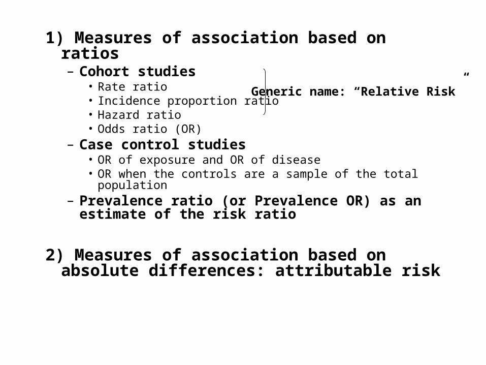
1) Measures of association based on ratios– Cohort studies
• Rate ratio• Incidence proportion ratio • Hazard ratio• Odds ratio (OR)
– Case control studies• OR of exposure and OR of disease• OR when the controls are a sample of the total
population– Prevalence ratio (or Prevalence OR) as an
estimate of the risk ratio
2) Measures of association based on absolute differences: attributable risk
Generic name: “Relative Risk”
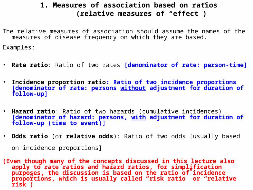
1. Measures of association based on ratios(relative measures of “effect”)
The relative measures of association should assume the names of the measures of disease frequency on which they are based.
Examples:
• Rate ratio: Ratio of two rates [denominator of rate: person-time]
• Incidence proportion ratio: Ratio of two incidence proportions [denominator of rate: persons without adjustment for duration of follow-up]
• Hazard ratio: Ratio of two hazards (cumulative incidences) [denominator of hazard: persons, with adjustment for duration of follow-up (time to event)]
• Odds ratio (or relative odds): Ratio of two odds [usually based on incidence
proportions]
(Even though many of the concepts discussed in this lecture also apply to rate ratios and hazard ratios, for simplification purposes, the discussion is based on the ratio of incidence proportions, which is usually called “risk ratio” or “relative risk”)

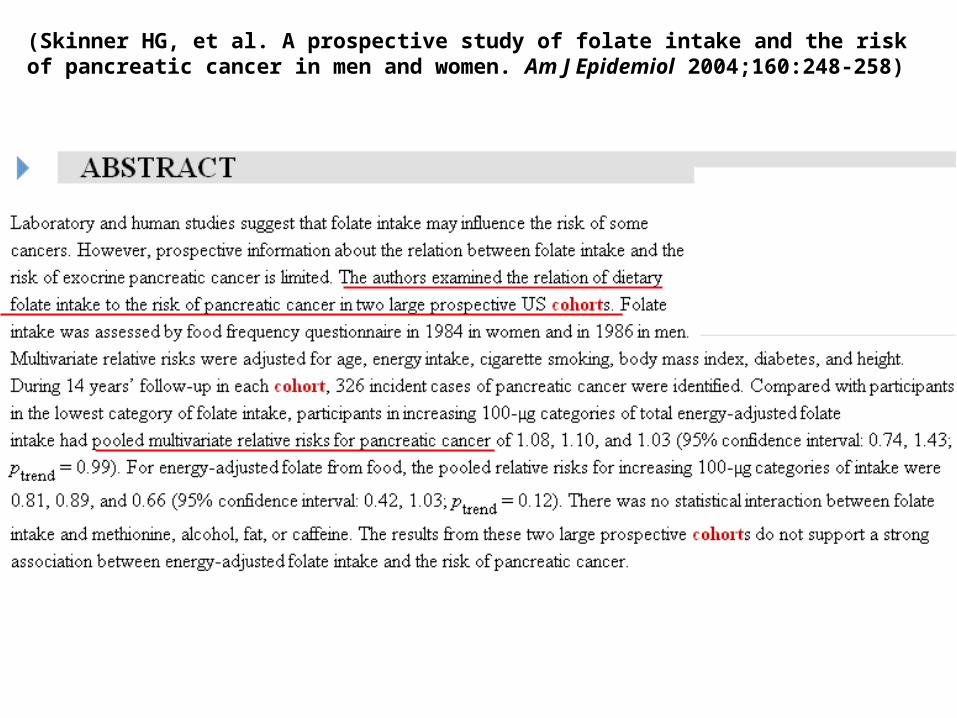
(Skinner HG, et al. A prospective study of folate intake and the risk of pancreatic cancer in men and women. Am J Epidemiol 2004;160:248-258)
(Skinner HG, et al. A prospective study of folate intake and the risk of pancreatic cancer in men and women. Am J Epidemiol 2004;160:248-258)

(Skinner HG, et al. A prospective study of folate intake and the risk of pancreatic cancer in men and women. Am J Epidemiol 2004;160:248-258)
Adjusts for multiple variables in addition to duration of follow-up (time to event)
=cumulative incidence

(Skinner HG, et al. A prospective study of folate intake and the risk of pancreatic cancer in men and women. Am J Epidemiol 2004;160:248-258)
“*Relative risks adjusted for potential confounders were approximated by Cox proportional hazards regression…”
** **
** Cases/Person-years= rates of pancreatic cancer

(Skinner HG, et al. A prospective study of folate intake and the risk of pancreatic cancer in men and women. Am J Epidemiol 2004;160:248-258)

Jacobs EJ, Multivitamin use and colorectal incidence in a US cohort: does timing matter? Am J Epidemiol 2003;158:621-628)

Jacobs EJ, Multivitamin use and colorectal incidence in a US cohort: does timing matter? Am J Epidemiol 2003;158:621-628)
Correct terminology? Incidence proportion ratios?Rate ratios?

Results
Wrong! It should be “hazard ratio”
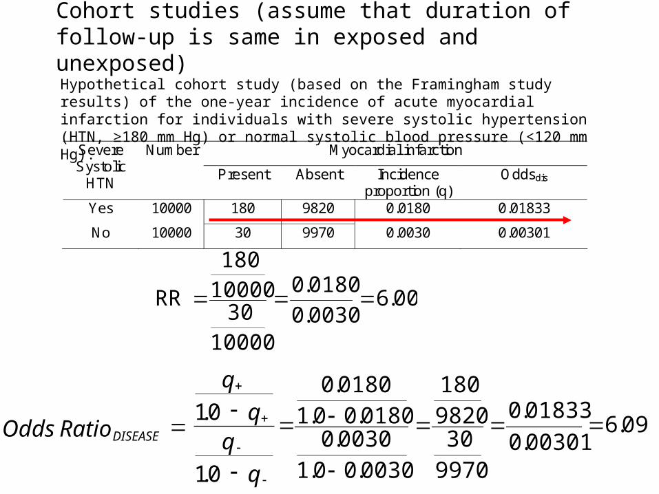
Cohort studies (assume that duration of follow-up is same in exposed and unexposed)
Myocardial infarction Severe Systolic
HTN
Number
Present Absent Incidence proportion (q)
Oddsdis
Yes 10000 180 9820 0.0180 0.01833
No 10000 30 9970 0.0030 0.00301
Hypothetical cohort study (based on the Framingham study results) of the one-year incidence of acute myocardial infarction for individuals with severe systolic hypertension (HTN, ≥180 mm Hg) or normal systolic blood pressure (<120 mm Hg).
09.600301.0
01833.0
997030
9820180
0030.00.10030.0
0180.00.10180.0
00600300
01800
1000030
10000180
...
RR
Odds Ratio
q
q
DISEASE
10
10
.
.
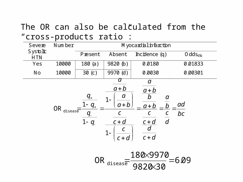
The OR can also be calculated from the “cross-products ratio”:
bc
ad
dcba
dcd
dcc
bab
baa
dccdc
cba
aba
a
1
1
1
1OR disease
09.6309820
9970180OR disease
Myocardial infarction Severe Systolic
HTN
Number
Present Absent Incidence (q) Oddsdis
Yes 10000 180 (a) 9820 (b) 0.0180 0.01833
No 10000 30 (c) 9970 (d) 0.0030 0.00301

When (and only when) the OR is used to estimate the risk ratio, there is a “built-in” bias:
09.6018.01
003.010.6OR dis
Myocardial infarction Severe Systolic
HTN
Number
Present Absent Incidence (q) Oddsdis
Yes 10000 180 (a) 9820 (b) 0.0180 0.01833
No 10000 30 (c) 9970 (d) 0.0030 0.00301
RR=6.0
OR=6.09
Example:
q
q
q
q
q
q
q
q
1
11
11
1OR
“bias”RR
09.6
997030
9820180
DISEASEOR
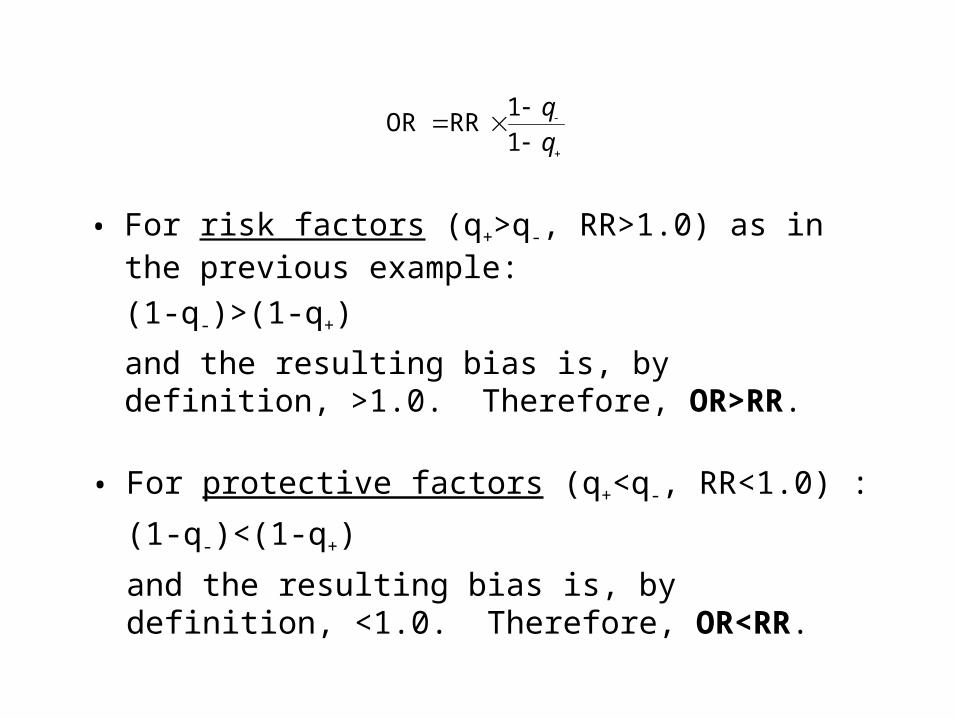
• For risk factors (q+>q-, RR>1.0) as in the previous example:
(1-q-)>(1-q+)
and the resulting bias is, by definition, >1.0. Therefore, OR>RR.
q
q
1
1RROR
• For protective factors (q+<q-, RR<1.0) :
(1-q-)<(1-q+)
and the resulting bias is, by definition, <1.0. Therefore, OR<RR.

IN GENERAL:
• The OR is always further away from 1.0 than the RR.
• The higher the incidence, the higher the discrepancy.

Relationship between RR and OR
… when probability of the event (q) is low:
or, in other words, (1-q) 1, and thus, the “built-in bias” term,
and OR RR.
q
1
0969820
997006
01801
0030106 .
.
..
.
..OR
Myocardial infarctionSevereSystolic
HTN
Number
Present Absent
Yes 10000 180 9820
No 10000 30 9970
Example:
096
997030
9820180
.OR 006
1000030
10000180
.RR
11
1 0
.
~1.0

Relationship between RR and OR
… when probability of the event (q) is high:
64.0
94.00.6
36.01
06.010.6OR
Recurrent MISevereSystolic
HTN
Number
Present Absent
Yes 10000 3600 6400
No 10000 600 9400
818
9400600
64003600
.OR 006
10000600
100003600
.RR
Example:Cohort study of the one-year recurrence of acute myocardial infarction (MI) among MI survivors with severe systolic hypertension (HTN, ≥180 mm Hg) and normal systolic blood pressure (<120 mm Hg).
q
0.36
0.06
= 1.47

OR vs. RR: Advantages
• OR can be estimated from logistic regression (to be discussed later in the course).
• OR can be estimated from a case-control study because…
…OR of exposure = Odds ratio of disease

CASE-CONTROL STUDIES
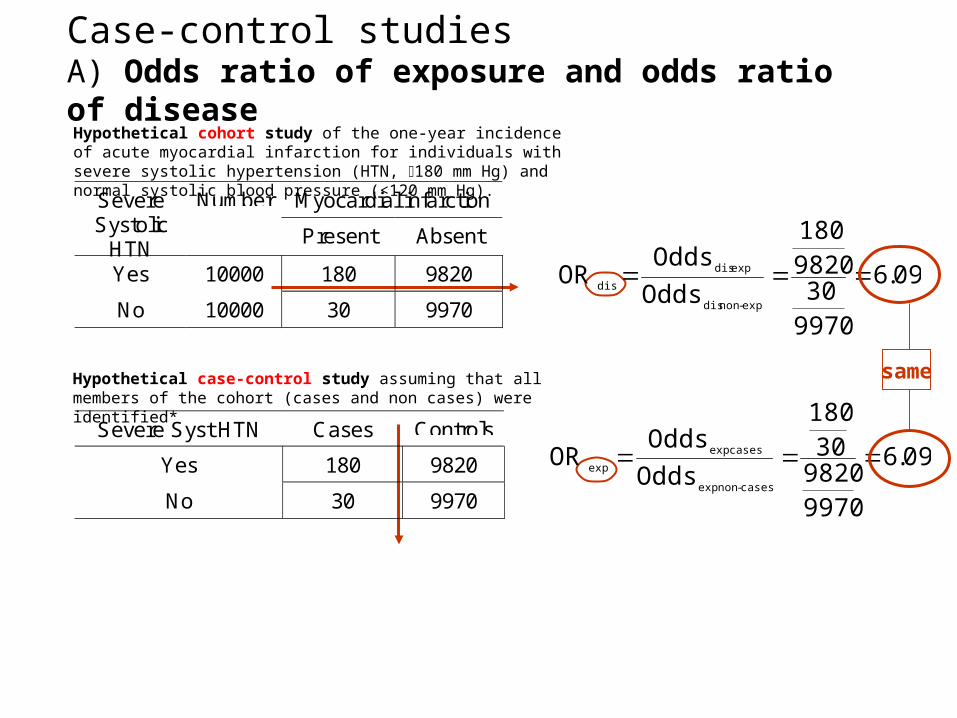
Case-control studiesA) Odds ratio of exposure and odds ratio of diseaseHypothetical cohort study of the one-year incidence of acute myocardial infarction for individuals with severe systolic hypertension (HTN, 180 mm Hg) and normal systolic blood pressure (<120 mm Hg).
Myocardial infarctionSevereSystolic
HTN
Number
Present Absent
Yes 10000 180 9820
No 10000 30 9970
096
997030
9820180
.Odds
OddsOR
exp-non dis
exp dis
dis
Hypothetical case-control study assuming that all members of the cohort (cases and non cases) were identified*
Severe Syst HTN Cases Controls
Yes 180 9820
No 30 9970
096
9970982030
180
.Odds
OddsOR
cases-non exp
cases exp
exp
same

Case-control studiesA) Odds ratio of exposure and odds ratio of disease
Retrospective (case-control) studies can estimate the OR of disease because:
ORexposure = ORdisease
Hypothetical cohort study of the one-year incidence of acute myocardial infarction for individuals with severe systolic hypertension (HTN, 180 mm Hg) and normal systolic blood pressure (<120 mm Hg).
Myocardial infarctionSevereSystolic
HTN
Number
Present Absent
Yes 10000 180 9820
No 10000 30 9970
096
997030
9820180
.Odds
OddsOR
exp-non dis
exp dis
dis
Hypothetical case-control study assuming that all members of the cohort (cases and non cases) were identified
Severe Syst HTN Cases Controls
Yes 180 9820
No 30 9970
096
9970982030
180
.Odds
OddsOR
cases-non exp
cases exp
exp
same
Because ORexp = ORdis, interpretation of the OR is always “prospective”.
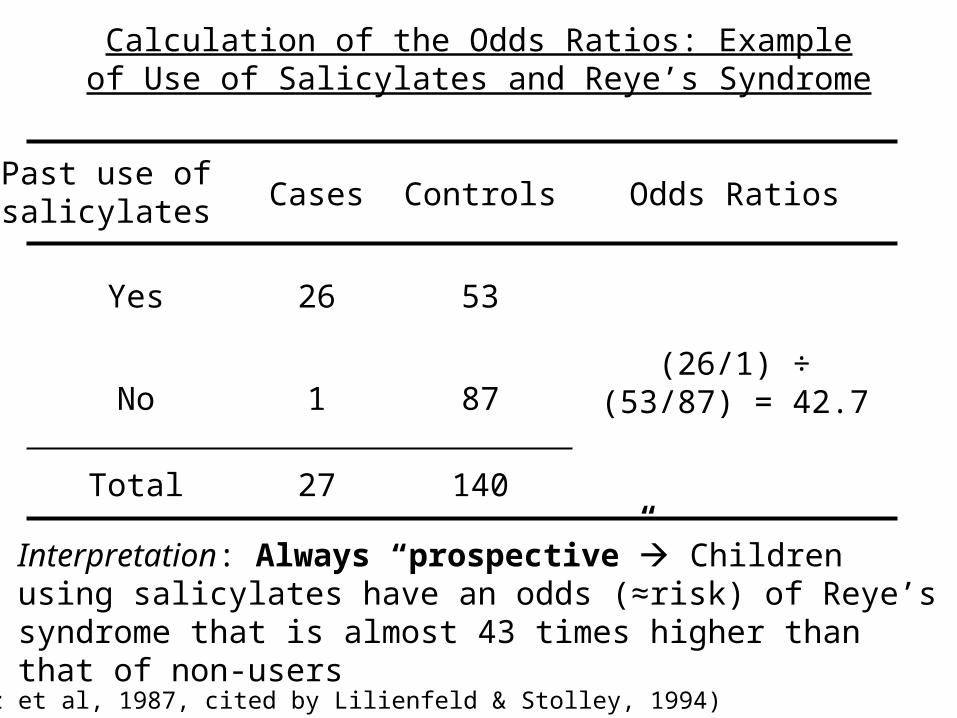
Calculation of the Odds Ratios: Example of Use of Salicylates and Reye’s Syndrome
14027Total
871No(26/1) ÷ (53/87) =
42.7
5326Yes
Odds RatiosControlsCases
Interpretation: Always “prospective” Children using salicylates have an odds (≈risk) of Reye’s syndrome that is almost 43 times higher than that of non-users
(Hurwitz et al, 1987, cited by Lilienfeld & Stolley, 1994)
Past use of salicylates

It is not necessary that the sampling fraction be the same in both cases and controls. As cases are less numerous, the sampling fraction for cases is usually greater than that for controls. For example, a majority of cases (e.g., 90%) and a smaller sample of controls (e.g., 20%) could be chosen (assume no random variability).
Severe Syst HTN Cases Controls
Yes 162 1964
No 27 1994
Toal 210 x 0.9 = 189 19790 x 0.2 = 3958
09.6
19941964
27162
ORexp
expexp
cntlsin
casesin
Odds
Odds
In a retrospective (case-control) study, an unbiased sample of the cases and controls (non-cases) yields an unbiased OR
Myocardial infarction Severe Systolic
HTN
Number
Present Absent
Yes 10,000 180 9,820
No 10,000 30 9,970
Total 20,000 210 19,790
O RO dds
O ddsd is
d is
d is un
ex p
ex p
.
1 8 0
9 8 2 03 0
9 9 7 0
6 0 9
Cohort study:

Case-control studiesB) OR when controls are a sample of the total population
In a case-control study, when the control group is a sample of the total population (rather than only of the non-cases), the odds ratio of exposure is an unbiased estimate of the INCIDENCE PROPORTION RATIO (or, if adjustment for duration of follow-up is done, of the HAZARD RATIO)
Risk factor CASES NON-CASES TOTALPOPULATION
Present a b a+b
Absent c d c+d
dbca
cases-non exp
cases expexp Odds
OddsOR
RR
Odds
OddsOR
population exp
cases exp
exp
dcc
baa
dcba
ca
00.6
000,10600
000,10600,3
RR
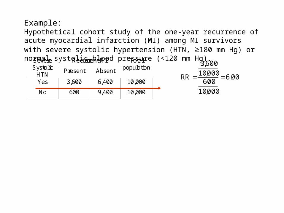
Example:Hypothetical cohort study of the one-year recurrence of acute myocardial infarction (MI) among MI survivors with severe systolic hypertension (HTN, ≥180 mm Hg) or normal systolic blood pressure (<120 mm Hg).
Recurrent MI Severe Systolic
HTN Present Absent
Total population
Yes 3,600 6,400 10,000
No 600 9,400 10,000

00.6
000,10600
000,103600
RR
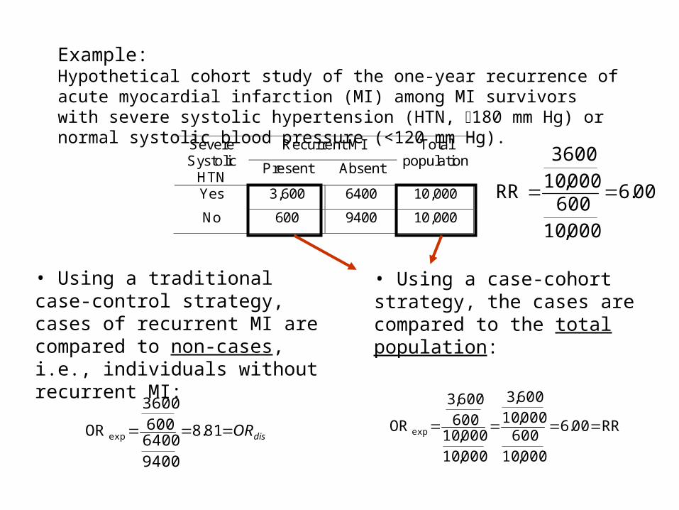
Example:Hypothetical cohort study of the one-year recurrence of acute myocardial infarction (MI) among MI survivors with severe systolic hypertension (HTN, 180 mm Hg) or normal systolic blood pressure (<120 mm Hg).
Recurrent MI Severe Systolic
HTN Present Absent
Total population
Yes 3,600 6,400 10,000
No 600 9,400 10,000
• Using a traditional case-control strategy, cases of recurrent MI are compared to non-cases, i.e., individuals without recurrent MI:
disOR 81.8
94006400600
3600
OR exp
00.6
000,10600
000,103600
RR
Example:Hypothetical cohort study of the one-year recurrence of acute myocardial infarction (MI) among MI survivors with severe systolic hypertension (HTN, 180 mm Hg) or normal systolic blood pressure (<120 mm Hg).
Recurrent MI Severe Systolic
HTN Present Absent
Total population
Yes 3,600 6400 10,000
No 600 9400 10,000
• Using a traditional case-control strategy, cases of recurrent MI are compared to non-cases, i.e., individuals without recurrent MI:
disOR 81.8
94006400600
3600
OR exp
• Using a case-cohort strategy, the cases are compared to the total population:
RR00.6
000,10600
000,10600,3
000,10000,10
600600,3
OR exp
Recurrent MI Severe Systolic
HTN Present Absent
Total population
Yes 3,600 6,400 10,000
No 600 9,400 10,000
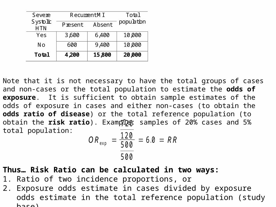
Total 4,200 15,800 20,000
O R R Rex p .
7 2 0
1 2 05 0 0
5 0 0
6 0
Thus… Risk Ratio can be calculated in two ways:1. Ratio of two incidence proportions, or2. Exposure odds estimate in cases divided by exposure odds estimate in the
total reference population (study base).
Note that it is not necessary to have the total groups of cases and non-cases or the total population to estimate the odds of exposure. It is sufficient to obtain sample estimates of the odds of exposure in cases and either non-cases (to obtain the odds ratio of disease) or the total reference population (to obtain the risk ratio). Example: samples of 20% cases and 5% total population:
Knuiman MW et al, Serum ferritin and cardiovascular disease: a 17-year follow-up study in Busselton, Western Australia. Am J Epidemiol 2003;158:144-149

Knuiman MW et al, Serum ferritin and cardiovascular disease: a 17-year follow-up study in Busselton, Western Australia. Am J Epidemiol 2003;158:144-149

Knuiman MW et al, Serum ferritin and cardiovascular disease: a 17-year follow-up study in Busselton, Western Australia. Am J Epidemiol 2003;158:144-149

Knuiman MW et al, Serum ferritin and cardiovascular disease: a 17-year follow-up study in Busselton, Western Australia. Am J Epidemiol 2003;158:144-149
* Barlow WE. Robust variance estimation for the case-cohort design. Biometrics 1994;50:1064-1072
*
Total cohort with serum samples: 1,612 individuals × 0.75= 1209

Knuiman MW et al, Serum ferritin and cardiovascular disease: a 17-year follow-up study in Busselton, Western Australia. Am J Epidemiol 2003;158:144-149
†Adjusted for age and other cardiovascular risk factors

To summarize, in a case-control study:
What is the control group?
What is calculated?
To obtain ...
Sample of NON-CASES
Odds
RatioDisease
Sample of the TOTAL POPULATION
Risk Ratio
cases-non exp
cases exp
exp Odds
OddsOR
pop total exp
cases exp
exp Odds
OddsOR

Recapitulation - I• Measures of association quantify a relationship between a potential risk
factor and an outcome• Measures of association adopt the names of the measures of disease
occurrence on which they are based:– Rate ratio: ratio of two rates (based on person-time)– Incidence proportion ratio: ratio of two incidence proportions (based
on persons)– Hazard ratio or Cumulative incidence ratio: ratio of two hazards
(based on persons, adjusted for time to event)– Odds ratio: ratio of two odds:
• In a cohort study, ratio of the odds of disease in exposed and in unexposed
• In a case-control study, ratio of the odds of exposure in cases and in controls
Odds ratio of exposure = odds ratio of disease; thus, interpretation of odds ratio in a case-control study is always “predictive” or “prospective”
NOTE: “RELATIVE RISK” IS A GENERIC NAME

Recapitulation - II
• The ideal ratio-based measure of association is the hazard ratio (cumulative incidence ratio):
– Its analytic unit is person;
– It adjusts for differential follow-up duration between the groups under comparison (e.g., exposed and unexposed, intervention and control);
– Using the Cox regression model, additional variables (that is, other than duration of follow-up) can be adjusted for;
– It can be estimated in a case-cohort study.

2) THEORETICALLY, RATES CAN RESULT IN IMPOSSIBLE VALUES
Example:
• One wishes to obtain a one-year case-fatality rate of disease Y, which is highly lethal.
• 50 persons are followed for up to one year:
-Deaths are relatively uniform over the one-year follow-up. Average follow-up for 40 (out of the 50) patients who die is 6 months
-6 individuals are (also uniformly) lost to follow-up after an average of 6 months
No. of person-years= (40 × 6/12) + (6 × 6/12) + (4 × 1)= 27
Recapitulation- IIIPROBLEMS WITH RATES, AND THUS RATE RATIOS, BASED ON USING TIME UNITS (E.G., PERSON-YEARS)
1) ASSUMPTION OF ACUTE (NON-CUMULATIVE) EFFECT: To follow N persons for t time is equivalent to following t persons for N time
-Person-time= N × t
Example: 20 SMOKERS FOLLOWED FOR 1 YEAR = 1 SMOKER FOLLOWED FOR 20 YEARS= 20 PERSON-YEARS
Rate (%) = (40 ÷ 27) × 100= 148/100 PY
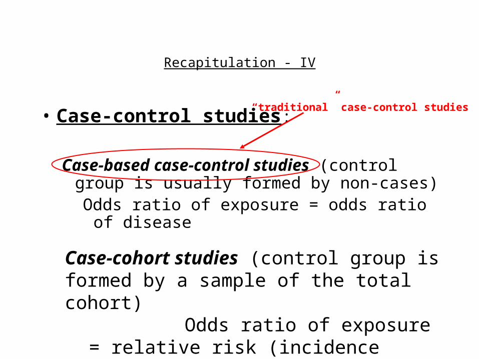
Recapitulation - IV
• Case-control studies:
Case-based case-control studies (control group is usually formed by non-cases)Odds ratio of exposure = odds ratio
of disease
“traditional” case-control studies
Case-cohort studies (control group is formed by a sample of the total cohort)
Odds ratio of exposure = relative risk (incidence proportion ratio or hazard ratio)

Risk factor CASES NON-CASES TOTALPOPULATION
Present a b a+b
Absent c d c+d
dbca
cases-non exp
cases expexp Odds
OddsOR
CASE-BASED CASE-CONTROL STUDYUSES A SAMPLE OF NON-CASES:
RR
Odds
OddsOR
population exp
cases expexp
dcc
baa
dcba
ca
CASE-COHORT STUDY USES A SAMPLE OF THE TOTAL COHORT (STUDY BASE):
TO CALCULATE THE RISK RATIO VIA INCIDENCE PROPORTIONS (OR RATES, OR HAZARDS), A CLASSICAL COHORT ANALYSIS IS NEEDED

Risk factor CASES NON-CASES TOTALPOPULATION
Present a b a+b
Absent c d c+d
dbca
cases-non exp
cases expexp Odds
OddsOR RR
Odds
OddsOR
population exp
cases expexp
dcba
ca
CASE-BASED CASE-CONTROL STUDYUSES A SAMPLE OF NON-CASES:
CASE-COHORT STUDY USES A SAMPLE OF THE TOTAL COHORT (STUDY BASE):
TO CALCULATE THE RISK RATIO IN A CASE-COHORT STUDY, ONLY AN ESTIMATE OF THE ODDS OF EXPOSURE IN THE TOTAL COHORT (STUDY BASE) IS NEEDED.
NOTE: IN A CASE-COHORT STUDY, BECAUSE THE OREXP = RR, THE “DISEASE RARITY” ASSUMPTION IS NOT NECESSARY
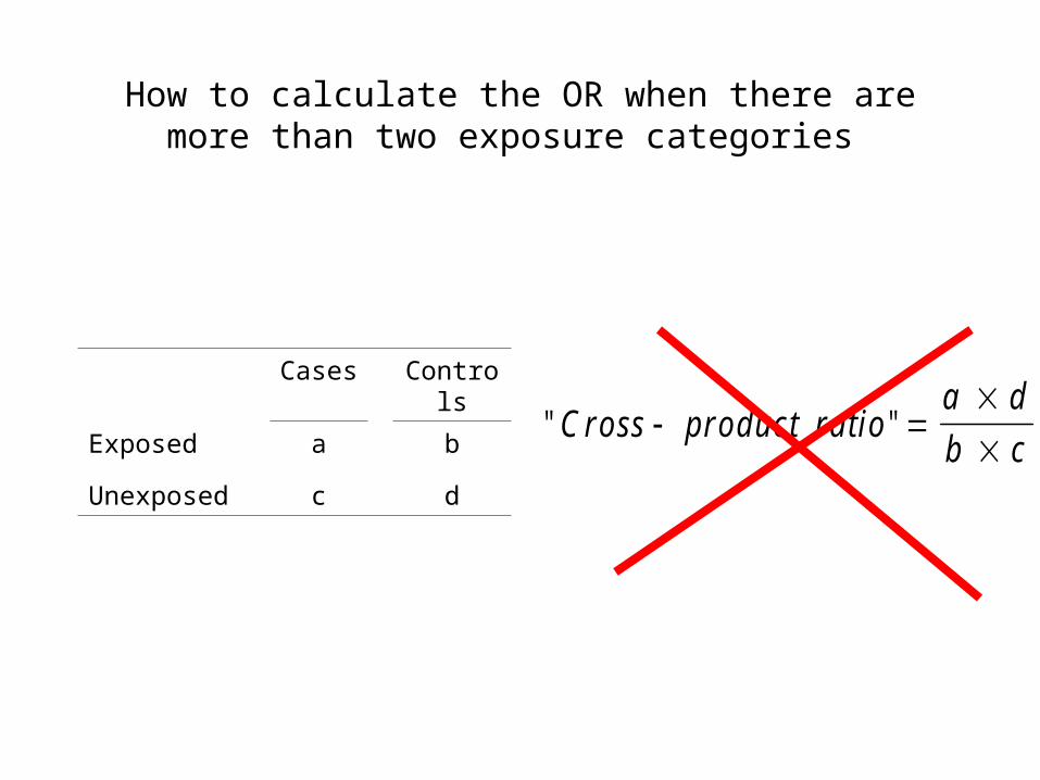
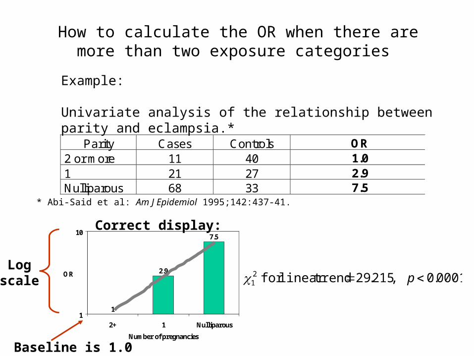
How to calculate the OR when there are more than two exposure categories
Cases Controls
Exposed a b
Unexposed c d
" "C ross product ra tioa d
b c

How to calculate the OR when there are more than two exposure categories
Example:
Univariate analysis of the relationship between parity and eclampsia.*
* Abi-Said et al: Am J Epidemiol 1995;142:437-41.
1
2.9
7.5
0
1
2
3
4
5
6
7
8
2+ 1 Nulliparous
Number of pregnancies
OR
Parity Cases Controls OR2 or more 11 401 21 27Nulliparous 68 33
1.0 (Reference)(21/11)÷(27/40)=2.9(68/11)÷(33/40)=7.5
Unexposed:
How to calculate the OR when there are more than two exposure categories
Parity Cases Controls OR2 or more 11 40 1.01 21 27 2.9Nulliparous 68 33 7.5
Example:
Univariate analysis of the relationship between parity and eclampsia.*
* Abi-Said et al: Am J Epidemiol 1995;142:437-41.
1
2.9
7.5
1
10
2+ 1 Nulliparous
Number of pregnancies
OR 0001.0,215.2921 ptrend linear for
Correct display:
Logscale
Baseline is 1.0

Detour…A statistical significant (or non-significant) trend test should not be automatically interpreted as proof of (or automatically disprove) the presence of a dose-response association.
Studies with small sample size may result in a NS trend test even though there appears to be a dose-response association
OR
Exposure level
1.0
N=80P(trend)=0.07
?Studies with large samples size may result on a significant trend test even though there is no dose-response association (threshold effect)
OR
Exposure level
1.0
N=80,000P(trend)=0.02

Detour…A statistical significant (or non-significant) trend test should not be automatically interpreted as proof of (or automatically disprove) the presence of a dose-response association.
Studies with small sample size may result in a NS trend test even though there appears to be a dose-response association
OR
Exposure level
1.0
N=80P(trend)=0.07
Studies with large samples size may result on a significant trend test even though there is no dose-response association (threshold effect)
OR
Exposure level
1.0
N=80,000P(trend)=0.02

A note on the use of estimates from a cross-sectional study (prevalence ratio, OR) to estimate the risk ratio
I
I
P
P
However, if exposure is also associated with shorter survival (D+ < D-), D+/D- <1 the prevalence ratio will underestimate the RR.
D
D
I
I
P-1PP-1
P
If this ratio~1.0
I
I
P
P
D
D
I
I
P
PIf the prevalence is low (~≤5%)
Real life example? Smoking and emphysema
Duration (prognosis) of the disease after onset is independent of exposure (similar in exposed and unexposed)...
Prevalence Odds=
R ISK R A T IO
P O IN T P R E V A L E N C E R A T IOyears
years
5 %
1 %5
5 %
1 %
2
42 5.
Hypothetical example:

2. Measures of association based on absolute differences
• Attributable risk in the exposed: The excess risk (e.g., incidence) among individuals exposed to a certain risk factor that can be attributed to the risk factor per se:
qqARexp
Or, expressed as a percentage:
100q
qq%AR
exp
100RR
1-RR%ARexp In
cid
en
ce (
pe
r 1
00
0)
Unexposed Exposed
Pop AR
ARexp

2. Measures of association based on absolute differences
• Attributable risk in the exposed: The excess risk (e.g., incidence) among individuals exposed to a certain risk factor that can be attributed to the risk factor per se:
qqARexp
Or, expressed as a percentage:
100q
qq%AR
exp
100RR
1-RR%ARexp
• Population attributable risk: The excess risk in the population that can be attributed to a given risk factor. Usually expressed as a percentage:
100q
qq%PopAR
npop'
npop'exp
Advantage: In case-control studies, the RR can be replaced by the OR
10011)(RRp
1)(RRp%PopAR
exp
expexp
*Levin: Acta Un Intern Cancer 1953;9:531-41.
Levin’s formula:*
The Pop AR will depend not only on the RR, but also on the prevalence of the risk factor (pexp)

Inci
de
nce
(p
er
10
00
)
Unexposed Exposed
Pop AR
ARexp
Population
IF EVERYONE IN THE REFERENCE POPULATION IS EXPOSED: PopAR = ARexp
Inci
de
nce
(p
er
10
00
)
Unexposed Exposed
Pop AR
ARexp
Population
IF NO ONE IN THE REFERENCE POPULATION IS EXPOSED: PopAR = Zero
Inci
de
nce
(p
er
10
00
)
Unexposed Exposed
Pop AR
ARexp
Population
IF A CERTAIN PROPORTION, BUT NOT ALL PERSONS IN THE REFERENCE POPULATION, ARE EXPOSED:PopAR < ARexp

Chu SP et al. Risk factors for proximal humerus fracture. Am J Epi 2004; 160:360-367
Cases: 448 incident cases identified at Kaiser Permanente. 45+ yrs old, ascertained through radiology reports and outpatient records, confirmed by radiography, bone scan or MRI. Pathologic fractures excluded (e.g., metastatic cancer).
Controls: 2,023 controls sampled from Kaiser Permanente membership (random sample).
Dietary Calcium (mg/day) Odds Ratios (95% CI)
Highest quartile (≥970) 1.00 (reference)
Lowest quartile (≤495) 1.54 (1.14, 2.07)
Interpretation: If those exposed to values in the lowest quartile had been exposed to values in the highest quartile, their odds (risk) would have been 35% lower.
Percent ARexposed%35100
54.1
154.1100
OR
1-OR100
RR
1-RR
~
Percent Population AR
p R R
p R R
p O R
p O Rex p
ex p
ex p
ex p
( )
( )
( )
( )
. ( . )
. ( . ). .
1
1 11 0 0
1
1 11 0 0
0 2 5 1 5 4 1
0 2 5 1 5 4 1 11 0 0 11 9 %~
RR estimate ~ 1.54Pexp ~ 0.25
10011)(RRP
1)(RRP
exp
exp
Levin’s formula for the Percent ARpopulation
Interpretation: The exposure to the lowest quartile is responsible for about 12% of the total incidence of humerus fracture in the Kaiser permanente population
What is the %AR in those exposed to the lowest quartile?
What is the Percent AR in the total population due to exposure in the lowest quartile?

EXAMPLE:
Risk of diarrhea in 36 Peace Corps volunteers in Guatemala:(based on data in Herwaldt et al: Ann Intern Med 2000;132:982-8)
Total=2521 person weeks, 307 diarrhea episodes (rp=0.122)
– Drank water of unknown source • Exposed: 594 pw, 105 episodes (r+=0.177/pw)
• Unexposed: 1927 pw, 202 episodes (r-=0.105/pw)
RR= 0.177 ÷ 0.105= 1.69
ARexp= 0.177 – 0.105= 0.072/pw; %ARexp= (0.072 ÷ 0.177) x 100= 40.7%
0.1050.122
0.177
0
0.05
0.1
0.15
0.2
Unexposed Population Exposed
Inci
denc
e (p
er p
erso
n-w
eek)
14%1000.122
0.1050.122100
r
rr%PopAR
pop
pop
Pex p .
5 9 4
5 9 4 1 9 2 70 2 3 6
%141000.1)0.169.1(236.0
)0.169.1(236.0%:'
PopARFormulasLevin
10011)(RRP
1)(RRP%PopAR :formula sLevin'
exp
expexp
CAUTION: THE ATTRIBUTABLE RISK SHOULD BE ESTIMATED ONLY WHEN THERE IS REASONABLE CERTAINTY THAT THE ASSOCIATION IS CAUSAL
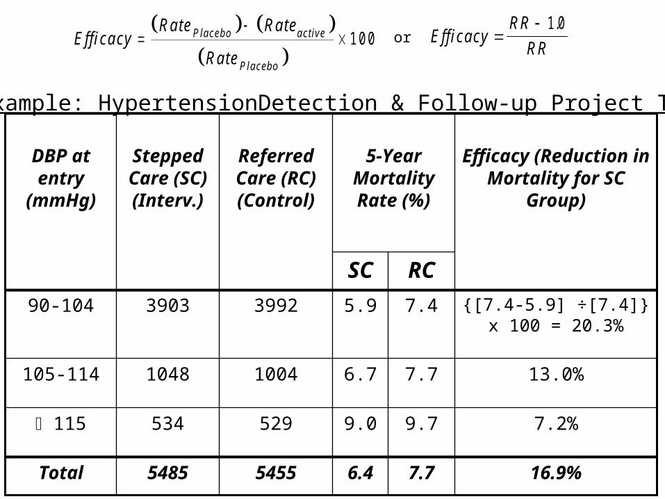
• Efficacy: the extent to which a specific intervention or service produces a beneficial result under ideal conditions. Ideally the determination of efficacy is based on results of randomized clinical trials (RCTs).
• Effectiveness: the extent to which a specific intervention or service, when deployed in the field, does what it is intended to do for a defined population.
• Efficiency– The effects or end-results achieved in
relation to the effort expended in terms of money, resources and time. The extent to which the resources used to provide a specific intervention or service of known efficacy and effectiveness are minimized. A measure of the economy (or cost in resources) with which a procedure of known efficacy and effectiveness is carried out.
– (In statistics, the relative precision with which a particular study design or estimator will estimate a parameter of interest.)
% E fficacy
Inc Inc
Inc
C ontro l In terven tion
C on tro l
1 0 02 0 % 1 0 %
2 0 %1 0 0 5 0 %
%. . .
.E fficacy
R R
R R
1 0 2 0 1 0
2 01 0 0 5 0 %
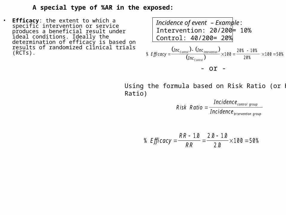
Incidence of event – Example:Intervention: 20/200= 10%Control: 40/200= 20%
- or -
R isk R atioIncidence
Incidencecon tro l group
erven tion group
in t
Using the formula based on Risk Ratio (or HazardRatio)
A special type of %AR in the exposed:
• Efficacy: the extent to which a specific intervention or service produces a beneficial result under ideal conditions. Ideally the determination of efficacy is based on results of RCTs.
• Effectiveness: the extent to which a specific intervention or service, when deployed in the field, does what it is intended to do for a defined population.
• Efficiency– The effects or end-results achieved in relation to
the effort expended in terms of money, resources and time. The extent to which the resources used to provide a specific intervention or service of known efficacy and effectiveness are minimized. A measure of the economy (or cost in resources) with which a procedure of known efficacy and effectiveness is carried out.
– (In statistics, the relative precision with which a particular study design or estimator will estimate a parameter of interest.)
• Efficacy: the extent to which a specific intervention or service produces a beneficial result under ideal conditions. Ideally the determination of efficacy is based on results of RCTs.
• Effectiveness: the extent to which a specific intervention or service, when deployed in the field, does what it is intended to do for a defined population.
• Efficiency– The effects or end-results achieved in
relation to the effort expended in terms of money, resources and time. The extent to which the resources used to provide a specific intervention or service of known efficacy and effectiveness are minimized. A measure of the economy (or cost in resources) with which a procedure of known efficacy and effectiveness is carried out.
– (In statistics, the relative precision with which a particular study design or estimator will estimate a parameter of interest.)

• Efficacy: Does the intervention work under ideal conditions?
• Effectiveness: If we implement the intervention in a “real life” situation, is it effective?
– Example:
• Efficacy of a vaccine= 90%
• Only 30% of individuals can tolerate its side effects; Thus...
• EFFECTIVENESS= 90% x 30%= 27%
• Efficiency: Cost-effectiveness ratio
E fficacyR a te R a te
R a te
P lacebo active
P lacebo
1 0 0
16.9%7.76.454555485Total
7.2%9.79.0529534 115
13.0%7.76.710041048105-114
{[7.4-5.9] ÷[7.4]} x 100 = 20.3%
7.45.93992390390-104
RCSC
Efficacy (Reduction in Mortality for SC
Group)
5-Year Mortality Rate (%)
Referred Care (RC) (Control)
Stepped Care (SC) (Interv.)
DBP at entry
(mmHg)
Example: HypertensionDetection & Follow-up Project Trial
E fficacyR R
R R
1 0.or