measurements on microtomographic images of fibrous structures
TRANSCRIPT

Measurements onmicrotomographic images of
fibrous structures
Jens Bache-Wiig [email protected] Christian Henden [email protected]
November 2004
Project report in TDT4725Image Processing specialization
Supervised by Professor Richard Blake
Faculty of Information Technology, Mathematics and ElectricalEngineering
Department of Computer and Information Science
Version 1.03


Preface
This is the report on a study conducted by two computer science major stu-dents at the Department of Computer and Information Science at the Norwe-gian University of Science and Technology. The study is part of preparatorywork for the master thesis. The project’s period was from the 16th of Au-gust to the 26th of November. The project assignment was specified by thePaper and Fibre Research Institute
The project was supervised by Prof. Richard Blake from the NorwegianUniversity of Science and Technology (NTNU), and Dr. Ing. Per Nygardfrom the Paper and Fibre Research Institute (PFI).
Structure of the report
The first chapter gives an introduction to the report and the main methods ofimage acquisition in the paper-science domain. Chapter two explains centralconcepts in computer science and looks at how to make the processing ofhigh-resolution, three-dimensional images more feasible. The third chaptergives an overview of the existing method of processing images of materialsamples. Improvements are suggested. Chapter four gives an overview ofmeasures done on these images in the paper science domain. The finalchapter introduces fractal analysis and looks at how it can be used to makemeasurements on images.
We specify which sections are our own work throughout the report. Eachchapter generally has two parts: a literature study and our own work, andin that order.
Intended audience and how to read this report
It has been assumed that the reader has a basic knowledge of computer sci-ence and mathematics. Concepts in paper science, physics, image analysisand graphics are explained where the understanding of these concepts arenecessary to understand other parts of the report. Concepts that are lesscentral are not explained, but the reader is given references that enables herto learn these concepts from other sources. This explanation of commonconcepts is necessary for the report to be read by people from all fields in-terested in the analysis of high-resolution microscopy images, which includesmaterial science, biology, chemistry, computer science and others. We haveincluded an index at the end of this document so that the reader may getback to definitions and explanations of concepts if necessary.

Acknowledgements
The authors would like to thank Richard Blake, Per Nygard, Øyvind Gregersenand Gary Chinga for their suggestions and feedback on the project. A specialthanks goes to Anneli Olsbø for proof-reading a draft of this report.
Abstract
Recent improvements in computer processing and storage capabilities havemade the analysis and visualisation of high-resolution three-dimensional im-ages of material samples possible. The structure of the material is of spe-cial significance to its properties, and has as such been an active area ofresearch. In order to analyse the structure, noise-reduction and binarisa-tion of the material images are necessary. We have examined the currentmethods of noise-reduction and binarisation and suggested improvements tothese. The different methods of quantification of material properties fromtheir images in the literature has been summarised and a new method ofstructure quantification based on fractal analysis is suggested.


Contents
Preface iv
Abstract v
1 Introduction 11.1 Background . . . . . . . . . . . . . . . . . . . . . . . . . . . . 11.2 Objective . . . . . . . . . . . . . . . . . . . . . . . . . . . . . 21.3 Image acquisition . . . . . . . . . . . . . . . . . . . . . . . . . 2
2 Volume graphics 72.1 Volumetric data . . . . . . . . . . . . . . . . . . . . . . . . . . 72.2 Visualisation . . . . . . . . . . . . . . . . . . . . . . . . . . . 92.3 Reducing storage demand . . . . . . . . . . . . . . . . . . . . 122.4 Improving performance . . . . . . . . . . . . . . . . . . . . . 162.5 Conclusions . . . . . . . . . . . . . . . . . . . . . . . . . . . . 18
3 Binarisation 193.1 Introduction . . . . . . . . . . . . . . . . . . . . . . . . . . . . 193.2 Current method of binarisation . . . . . . . . . . . . . . . . . 193.3 Discussion of current method . . . . . . . . . . . . . . . . . . 223.4 Suggested improvements . . . . . . . . . . . . . . . . . . . . . 233.5 Preliminary results and discussion . . . . . . . . . . . . . . . 26
4 Feature extraction 334.1 Existing methods . . . . . . . . . . . . . . . . . . . . . . . . . 334.2 New methods . . . . . . . . . . . . . . . . . . . . . . . . . . . 434.3 A practical application of feature extraction . . . . . . . . . . 434.4 Relevance to new materials . . . . . . . . . . . . . . . . . . . 444.5 Discussion and future work . . . . . . . . . . . . . . . . . . . 45
5 Fractal analysis 475.1 Introduction . . . . . . . . . . . . . . . . . . . . . . . . . . . . 475.2 Mathematical foundation . . . . . . . . . . . . . . . . . . . . 485.3 Fractal dimension as a descriptor . . . . . . . . . . . . . . . . 49
vii

viii Contents
5.4 Estimating the fractal dimension . . . . . . . . . . . . . . . . 505.5 Fractal dimension and roughness . . . . . . . . . . . . . . . . 555.6 Discussion and future work . . . . . . . . . . . . . . . . . . . 58
6 Conclusion 59
A Implementation 61A.1 SUSAN plugins . . . . . . . . . . . . . . . . . . . . . . . . . . 61A.2 Plugins for fractal analysis . . . . . . . . . . . . . . . . . . . . 62
Bibliography 65

Chapter 1
Introduction
This chapter establishes the background for our report. The two main meth-ods for high-resolution, three-dimensional image acquiring are presented andcompared.
1.1 Background
In material science it is desirable to learn more about how material propertiesat the micro level influence the macroscopic level (Holmstad et al. 2003).Manual or automated image analysis of three-dimensional images of materialsamples is a useful tool in this respect. Automated analysis has the potentialto be more exact, reliable and objective than subjective analysis.
Fibre structures are generally highly interwoven, porous three-dimensionalstructures. To give a complete analysis of such structures it is reasonablethat we should base our measurements on fully three-dimensional data. Onlyrecently has the technology for acquiring and processing large image volumesmade such studies practical. Yang (2001) advocates that the third dimensionis an important factor in dealing with thick fibrous materials, and that usingfully three-dimensional volume images will bring major improvements in theanalysis of fibre structures.
Several previous projects at PFI , the Norwegian Paper and Fibre ResearchInstitute, have focused on analysing microscopic images of paper. Someof the most recent contributions include (Holmstad 2004, Arns et al. 2004,Wang et al. 2004, Holen and Hagen 2004). In order to compare differentmaterial samples, a quantification of material properties based on the imagesof the material samples is calculated. PFI is planning to extend these effortsto other materials, such as cellulose-composites and fibre-based absorbentmaterials. This calls for a summary and evaluation of existing techniques, as
1

2 Chapter 1. Introduction
a thorough understanding of existing techniques is assumed to better enablethe adaption of existing methods and development of new methods for usein the analysis of new materials.
1.2 Objective
The project aims to give an overview of the current state of feature extractionfrom three-dimensional tomographic images of paper, including the processof preparing the images for feature extraction. If possible, these areas shouldbe extended and improved upon. The feature fractal dimension is such anextension of special interest in that regard.
A study of techniques for reducing the resource demands associated with theanalysis of high-resolution three-dimensional images should be performed inorder to make such analyses more feasible.
The report should aim to be comprehensible for paper scientists.
1.3 Image acquisition
The quality of an image depends on the method by which it is acquired.The way our image data is acquired, is perhaps the most unique aspect ofthe research presented in this report. Because a basic understanding of theacquisition is assumed in many of the following chapters, we will present itin this section.
There are several methods for acquiring high resolution three-dimensionalimage data. Some common examples are Confocal laser scanning microscopy(CLSM), scanning electronic microscopy (SEM) or light microscopy (LM)combined with serial sectioning, magnetic resonance imaging (MRI), andX-ray micro tomography. According to Holmstad (2004, p. 86), the pre-ferred technique for acquiring three-dimensional is X-ray micro tomographybecause “it gives access to the paper structure non-invasively at a uniformhigh resolution and contrast in all spatial directions and all parts of theimaged paper volume”.
Unlike SEM- or LM-based techniques based on serial sectioning, one doesnot have to cut into the material in order to obtain image slices. Thisavoids distortion between image slices, and simplifies the reconstruction ofthe digital volume.
The other applicable methods have either varying contrast or resolution inthe different spatial directions. For instance, all invasive techniques require

1.3. Image acquisition 3
precise cutting of cross sectional slices through the material. Even thoughsuch methods often give better quality images and a higher resolution foreach slice, it is difficult to achieve good resolution along the direction of thesectioning. Hence, the resulting voxels are oblong, complicating the dataanalysis.
The main disadvantages of X-ray tomography is its currently high cost andlow availability. Desktop-sized equipment exists, but supplies lower resolu-tion images than currently available large synchrotron sources. Accordingto Holmstad (2004), the current achievable resolution is roughly 5µm, butfuture developments will likely make high resolution X-ray tomography moreaffordable and available.
1.3.1 X-ray micro tomography
The creation of three-dimensional tomographic volumes with resolution con-siderably below the centimetre scale is commonly referred to as micro to-mography (X-µCT). Resolution below 1µm require high energy photons withgood penetration abilities. The X-ray beam also requires a high degree ofprecision. These properties are currently only achievable through the use ofa large, circular particle accelerator known as a synchrotron (Holmstad 2004,p. 86).
Figure 1.1: The basic principle behind X-ray tomography. Figure reproducedfrom http://www.esrf.fr
Figure 1.1 shows the basic working principle of X-ray tomography. A seriesof projected images are formed from the X-rays passing through the sample,while the sample is being rotated 180◦. This results in a projected radiographfor every angle. The set of radiographs are used to reconstruct the three-dimensional structure by solving a Fourier-like integral, known as the Radontransform (Holmstad 2004, p. 81).

4 Chapter 1. Introduction
Sample preparation
Samples are prepared by cutting out a small rectangular material sample.The sample is then mounted on a thin capillary by using melted glue. Thecapillary and the glue are highly visible features in the resulting data (fig-ure 1.2).
Figure 1.2: Typical absorption mode image showing the fibre structure, capillaryand glue.
There are two different methods that can currently be used to generate theprojection images. These methods are complimentary, in that they have dif-ferent properties, and can be used for different purposes. The two methodsare presented in the following sections. The images available to us are ob-tained at the European Synchrotron Radiation Facility (ESRF), beamlinesID-22 and ID-19. The size of the sampled volume is roughly 1mm3. Theexact dimensions will depend on the particular material sample.
Absorption mode imaging
Different contrast in absorption mode images reflects different levels of beam-absorption in the material. The absorption level is generally determinedby the average atomic density of the material. Figure 1.3 illustrates thisprocedure. This process is analogous to the X-ray images normally usedin hospitals, where bone structure results in a higher intensity than softertissue. Unfortunately some organic materials studied at PFI do not haveenough absorption contrast to make this method efficient. The resolutionobtainable by this technique at ESRF is approximately 0.7µm.
Phase contrast imaging
Phase contrast imaging is illustrated in figure 1.4. In phase-contrast imag-ing the amplitude of the signal is, according to constructive and destructive

1.3. Image acquisition 5
Figure 1.3: Illustration of absorption mode imaging. Figure reproduced fromhttp://www.esrf.fr
interference of the X-ray waves, refracted at phase borders in the sample(Holmstad 2004, p. 95), in other words high contrast in the resulting imagerepresents a border between regions of a different refractive index. The res-olution obtainable by this technique at ESRF laboratories, is approximately0.35µm.
Figure 1.4: Illustration of phase-contrast imaging. Figure reproduced from http://www.esrf.fr
Comparison and discussion
Image data generated by near-field phase-contrast, which contain only regionboundaries, are generally more difficult to binarise than data generated byabsorption mode. To binarise such volumes, regions must be filled. Thisfilling-procedure is complicated by the region boundaries being broken upby noise and other processes. Absorption mode imaging results in completeregions and does not require region-filling.
The advantage of using phase-contrast imaging to absorption mode is thatit has a higher spatial resolution. For some lighter materials, phase-contrastis still the only feasible method available.

6 Chapter 1. Introduction
The binarisation of phase contrast images is thoroughly treated in Antoineet al. (2001). The article gives a 23-step procedure for manual binarisation ofsuch images. The key points in this procedure are three-dimensional smooth-ing by averaging, low-pass Butterworth filtering in the frequency domain,median filtering and local thresholding (a thorough treatment of these con-cepts is given by Sonka et al. (1999)). In the mentioned procedure, seedingpoints has to be manually selected for each fibre of interest in every ninthimage slice, in order to fill the regions in the volume. Another drawbackis the extensive use of low-pass filtering, which significantly reduces imagedetails.
Prior research in the field has mostly concentrated on the processing of phasecontrast data, as it has been assumed (Antoine et al. 2001, Ramaswamyet al. 2001) that X-ray imaging of organic fibrous materials like paper re-quires the use of phase-contrast imaging. Recent advances at ESRF, beamline ID-19, resulted in absorption mode images with a better contrast thanpreviously assumed achievable. Using absorption mode is the preferredmethod due to the simpler processing. Although phase-contrast imagingcan provide higher spatial resolution than absorption mode, the effectiveresolution is degraded by the amount of filtering necessary to binarise thedata in the images. Recent research (Goel et al. 2004, Holmstad 2004), haveconcluded that absorption mode X-ray micro tomography is well suited forthe determination of quantitative measures of the paper structure.
Holmstad (2004, p. 138) discourages further development of image process-ing of near-field phase-contrast three-dimensional images. Because of thepromising results achieved using absorption mode imaging and Holmstad’srecommendation, we will focus on the processing of absorption mode imagesin the rest of this report.

Chapter 2
Volume graphics
This chapter aims to give a brief overview of how to handle volumetric imagedata in a resource-saving manner. We will start by defining some generalconcepts relating to volume graphics. We will also give an overview of howto visualise such data and investigate general methods on how to efficientlystore and process them.
2.1 Volumetric data
The main division in computer graphics goes between discrete and continu-ous representations. Three-dimensional computer graphics are often basedon continuous representations, but to measure quantities in the real world,we have to make discrete measures. Digital photography is a typical ex-ample, where the light is measured only at discrete intervals across a largematrix.
Volumetric data is typically a set S of samples (x, y, z,w), representing thevalue w of some property at a specific location (x, y, z). If the range of valuesis restricted to either 0 or 1, we refer to such data as binary data.Alternatively the value may represent some measurable property of the data,including grey-level or atomic density at each location. In the case of mul-tispectral data, e.g. colour images, the data is described by multiple sets.
In general such samples may be taken at random locations in space, butin most cases the set S consists of samples taken at regularly spaced in-tervals along three orthogonal axes. When the interval on each axis is ofequal length, the set S is called isotropic, otherwise it is called anisotropic(Kaufman 1994). It is most common to store such structures in a three-dimensional array, with the element location used to indicate its positionon the grid. The set S will be referred to as the array of values S(x, y, z) ,
7

8 Chapter 2. Volume graphics
defined only on grid-locations. If we consider the grid-locations to be centre-points on equally spaced cuboids1 or cubes, the individual cubes are oftenreferred to as voxels. Digitised image elements (the two-dimensional case)are commonly referred to as pixels.
2.1.1 Sampling and transformations
Since the set S is only valid at discrete intervals, a function ip(x, y, z) thatgives an estimate of the value at any continuous location may be needed. ipmust be defined so that ip = S on grid locations, but on non grid locationsip returns the value interpolated from nearby grid locations. The simplestsuch function is the nearest neighbour method, also called zero order inter-polation, that simply returns the value of the voxel containing it. First orhigher order interpolations can be used to achieve better approximations.
Figure 2.1: Demonstration of the problems associated with voxel transformations
A considerable problem with discrete representations is that they are notori-ously difficult to transform. This includes our pixels and voxels. A thoroughtreatment of pixel coordinate transformations can be found in Sonka et al.(1999). This explanation is easily extended to voxels as well. Any transfor-mation applied requires that data is fitted onto another discrete voxel-grid,and this is usually not a simple one-to-one mapping. For each grid point inthe target grid, a sample is taken at the transformed location in the originalgrid. Because this transformed point tends to not be exactly centred ona voxel, an interpolation is necessary, and can be performed by using thefunction ip(x, y, z) defined in the previous paragraph.
Figure 2.1 demonstrates how discrete data is affected by rotating a line
1Also known as a rectangular parallelepipeds

2.2. Visualisation 9
35◦clockwise and back again using voxel transformation. The upper rowshows the transformation performed using zero order interpolation, whilethe second row shows the result from a first order interpolation routine.Much information about the original voxel configuration is lost in the process(figure 2.1).
Figure 2.2: 26-adjacent (1), 18-adjacent (2) and 6-adjacent (3) voxels
2.1.2 Adjacency and connectedness
According to Kaufman (1994), two voxels are said to be 26-adjacent if theyshare either a corner, and edge or a face. Voxels that share either an edgeor a face are said to be be 18-adjacent and those sharing only a face aresaid to be 6-adjacent. These N-adjacencies are illustrated in figure 2.2. Theequivalent adjacencies for two-dimensional pixel-grids are the 4-adjacent and8-adjacent pixels, sharing either edges or both edges and corners respectively.We define the prefix N to define a particular adjacency relation. A sequenceof voxels that share a common property where all consecutive voxels areN-adjacent, is an N-path. A set W of voxels is called N-connected if thereis an N-path between every pair of voxels in W.
2.2 Visualisation
In order to discover new correlations between physical properties from three-dimensional images of the material, human experts may benefit from anaccurate visual representation of the image data, as this can improve theexpert’s understanding of the material structure. The simplest form of rep-resentation is to present consecutive image slices while scrolling through thevoxel volume in different directions. This will only yield a limited three-dimensional representation, and is not dependent on defining a surface be-cause we are in effect looking inside the material.
Several other forms of visualisation have been presented in Kaufman (1994).These are strictly divided into surface rendering techniques and volume ren-

10 Chapter 2. Volume graphics
dering techniques. The above mentioned techniques are explained in thefollowing sections.
2.2.1 Surface rendering techniques
This technique requires the explicit definition of a surface. A defined sur-face requires that the data have been successfully binarised, as described inChapter 3 and that a procedure known as surface fitting is applied. Surfacefitting consists of mapping geometric primitives onto the binarised data sothat a surface is created between objects and void. Because the surface is acontinuous structure, we must use some principle of interpolation betweenthe discrete sample grid.
When zero order interpolation is used on the voxels, squares are mapped ontothe voxels wherever a boundary between object and background is detected.Such simple geometrical primitives are often referred to as polygons. Adepth order algorithm is used to draw shaded squares onto the image plane.The result is a blocky, but comprehensible, image. This blocky image isunsuitable for assessment of optical properties, because light beams hittingvoxels will be reflected only at 90◦angles.
Surface mappings of higher quality can be achieved by defining the surfaceusing higher order interpolation. Such surfaces are known as iso-valuedsurfaces. For accurate simulation of optical properties, it is necessary thatgood approximations of an iso-valued surface is made. One of the mostpopular algorithms is the Marching Cubes algorithm, introduced by Lorensenand Cline (1987). It approximates iso-surfaces by limiting the ways a surfacecan pass through a voxel to one of 256 different predetermined polygonconfigurations, including triangular polygons. By symmetry this numbercan be reduced to 15 unique configurations, each stored in a look-up table.Each voxel is then mapped onto one of these configurations. By calculatingthe face normals for each triangle, and then generating averaged normals ineach corner of each polygon with its neighbours, a smooth looking surfacecan be rendered.
Holmstad (2004) concludes that the great amount of surface data generatedby the marching cube algorithm prohibited the inspection of the entire imagevolume acquired through synchrotron X-ray tomography, on current com-modity hardware. However, larger memory capacity and rapidly improvingsurface graphics acceleration, will probably make real-time inspections ofiso-surface data from tomographic images a reality.
The improvement of iso-surface mappings is an area of active research.

2.2. Visualisation 11
Figure 2.3: Volume rendering of a human head
2.2.2 Volume rendering
Instead of rendering the volume by defining a surface first, we can renderthe volume in a translucent manner, taking into account the brightness ofthe material beneath the surface. Figure 2.3 shows a volume rendering of ahuman head, created by using the Julius2 framework.
One such technique, based on ray casting is described in Levoy (1988): sur-face shading calculations are performed at every voxel with local gradientvectors serving as surface normals. Surface classification operators are thenapplied to obtain a partial opacity for every voxel. The resulting colour andopacity of each pixel in the image plane is blended from back to front bytracing rays from each pixel on the image plane. The result is a semitrans-parent, three-dimensional image of the volume. This technique is particu-larly suitable when amorphous phenomena such as clouds, fog and fire arerepresented.
2A software framework for the development of medical visualisation tools. More infor-mation can be obtained from their website at http://www.julius.caesar.de

12 Chapter 2. Volume graphics
2.3 Reducing storage demand
Images and volumes need to be stored in computer memory to be processed.The computer’s memory is a limited resource.
We define a byte to be a unit of storage containing 8 bits, each representingeither the value 1 or 0. We will use the tradition within computer science todescribe a kilobyte (KB) as exactly 1024 bytes, a megabyte (MB) as 10242
bytes and a gigabyte (GB) as 10243 bytes.
The number of voxels in an isotropic volume increases rapidly with increasingresolution. While a large, uncompressed two-dimensional image of dimen-sions 4096 × 4096 and 16 bits to represent each pixels intensity value needs4096 · 4096 · 16bits = 32MB of storage, a three-dimensional image with thesame resolution along the z-axis requires 32MB · 4096 = 128GB of storage.
The latter size is significantly larger than the size of the working memoryfound on commodity computers today, which typically allows a maximumof 4GB addressable primary storage memory. In modern memory architec-tures, primary memory is typically divided into several stages where smallerand faster memory sizes operate at a higher speed than larger, slower mem-ory types. This process is called caching. Additionally, most operatingsystems allow large data to be seamlessly swapped in and out of workingmemory in a process called swapping. Both these processes are based onspatial locality in the data to be accessed, in order to keep the number ofaccesses to slower larger media to a minimum. It is therefore necessary for anstorage-demanding algorithm to exploit spatial locality in order to achievemaximum efficiency.
In our case, we seek to process 8-bit isotropic volumes of size 2048×2048×256,which require3 1.0GB of storage. When processing an image it is commonthat more data than just the image need to be stored in the computer’smemory at some point in the process, making the effective requirement some-where above 1.0GB. Based on this we have investigated means of reducingstorage requirements in the following sections.
2.3.1 Compression of volumetric data
Because the size of the raw data makes them difficult to handle, it wouldbe desirable to compress them so that they require less storage space. Wewill therefore examine some common methods for the compression of voxelstructures in this section.
3Although volumes can have a larger number of xy-planes than 256 (slices), the originalvolumes are split into N volumes of 256 slices each to facilitate transport of the data.

2.3. Reducing storage demand 13
All kinds of data compression can be divided into two principal groups: thosethat are information-preserving and those that are“lossy”(Sonka et al. 1999)Information-preserving compression enables error free reconstruction, whilelossy methods will introduce some form of error. The compression obtainablethrough lossy compression tends to have substantial advantages with littleor no visible impact on the data. However, we consider them unsuitable forscientific use, because they may affect results in an unpredictable manner.
Octrees
A popular, information-preserving method for storing voxel data is the oc-tree. Octrees achieve image compression by storing information in a hier-archical tree structure. This structure is built by recursively subdividinginhomogeneous regions of the volume into eight sub-regions. This procedureis repeated until each terminal node of the tree corresponds to a region ofthe volume, in which all voxels are uniform or connected. This technique ismost efficient when the data is sparse, and large homogeneous regions arepresent (Samet and Webber 1988).
One disadvantage of an octree is the time it takes to construct the tree.Additionally, the tree must be reconstructed whenever we want to change oradd something to the structure. Even small variations on the input can resultin a very different tree (Samet and Webber 1988). The time used to maintainthe tree structure, can be reduced significantly by keeping changes to thestructure in a queue, and only periodically rebuild the actual tree structure.Any algorithm requiring mostly read access to its data will probably benefitfrom using this structure.
2.3.2 Implementing space-efficient image information stor-age
This section formalises our mentioned storage demand problem (see Sec-tion 2.3) and suggests how to solve it.
There are primarily two types of data that we want to access.
1. 8-bit volumes (originals)
2. Binarised volumes (processed)
Segmentation is the process of separating different parts of an image intodifferent classes. In the case where the segmentation results in two classesonly, the result is called a binarisation of the image.

14 Chapter 2. Volume graphics
Binary data is the result of applying the binarisation process described inChapter 3 to original tomographic image data. The original data sets areroughly 109 voxels in size, c.f. Section 2.3. The size may vary somewhat sowe will use it as an estimate only.
This distinction is useful because the original volumes may be processed bya high-end workstation, but the binary images should be usable to scientistsusing commodity workstations.
Storing 1.0–2.0 GB of data is within reasonable limits on modern graphicalworkstations. This makes cache optimisation the most critical motivationfor selection of an efficient storage structure. The simplest way to storesuch data is in a three-dimensional array, indexable by the grid coordinatesx,y,z. This will effectively result in a linear representation on disk, whereconsecutive image cross-sections (slices) are stored as a series of horizontalrows.
If the particular algorithm requires access to a local neighbourhood arounda single voxel element, many cache misses will occur because data fromdifferent image slices are spread out on disk. Interleaving image slices orsplitting up the data in smaller cubic structures may increase cache efficiency.
If the whole volume does not fit in the workstation’s memory, the data mustbe separated into smaller units, such as image slices or smaller blocks calledpages. We then load as many pages as possible, and load and unload pageson demand. This is commonly called .
Storing the binary data
Binary data can be stored using only 1 bit per pixel. Because the smallestaddressable unit on most modern CPUs is a single byte, we must pay forthis reduction in storage space by adding extra complexity to the access ofeach individual voxel. However, because more data will fit into the fastercache memory, it can potentially make calculations faster.
Extra calculations are required to isolate a single bit whenever a voxel isaccessed. However, this enables us to store 8 times as much data in thesame amount of memory.
The particular mapping from eight voxels to a single byte must be decidedupon. The mapping should exploit spatial locality to utilise the computer’scache for improved performance.
We have proposed two different mappings for this purpose in more detail.
1. A cube consisting of 2 × 2 × 2 voxels mapped onto a single byte

2.3. Reducing storage demand 15
2. Let bits increase along one of the coordinate axis, for example for each(x,y). The value of (x,y,z) is stored for 8 successive z-values.
The first has the advantage that it can be directly used to represent levels inan octree. The second has the advantage of having several slices in parallelaccessed at the same time. Because data are stored linearly in memory,this mapping may increase cache efficiency whenever data is accessed acrossseveral volume slices. This is the case when spatial averaging over adjacentvoxels is applied.
If the dimension of the total data is not an exact multiple of 8 in eitherdirection, it is necessary to pad out the extra data with zeros.
The two mappings mentioned are described in more detail in the followingsections.
2-cube mapping. The 2-cube mapping is done by first finding the cubewhich stores the voxel value and then finding the value (bit) of interest inthe particular cube.
This is the mapping from pixel coordinates to 2-cube coordinates:
xcube = bx2c (2.1)
ycube = by2c (2.2)
zcube = bz2c (2.3)
When the 2-cube that holds the pixel is found by equations (2.1) through(2.3), a mapping from pixel coordinates to bit number must be done. Thismapping is given by equation 2.4, where mod is the remainder operator,modulo.
pos(x, y, z) = 4(x mod 2) + 2(y mod 2) + (z mod 2) (2.4)
The mapping is visualised in figure 2.4.
8-vector mapping. As for the 2-cube mapping, the vector (byte) con-taining the pixel must be found first, and then the bit-number of the pixelmust be found.
This is the mapping from pixel coordinates to 8-vector coordinates:
xvector = x (2.5)yvector = y (2.6)
zvector = bz8c (2.7)

16 Chapter 2. Volume graphics
xi+1
yi+1 yi+1
zi zi+1
5 7
0
4 6
2 1 3
xi+1
xi
yi
xi
yi
Figure 2.4: Mapping of bit number (big-endian) to placement in cube
When the 8-vector that holds the pixel is found by equations (2.5) through(2.7), a mapping from pixel coordinates to bit number must be done. Thismapping is given by equation 2.8.
pos(x, y, z) = z mod 8 (2.8)
2.4 Improving performance
Due to the great amounts of data associated with tomographic imaging,efficient processing is critical. Processing time can be reduced by solvingparts of the image processing problem in parallel. Parallelism is applicableto many problems and new technologies have made parallel computationavailable even on desktop workstations. In light of this we focus on parallelmethods of computation in this section, in addition to native optimisationswhich is a field that has seen some changes after the introduction of cross-platform code that newer high level languages, like Java produces.
2.4.1 Parallel and distributed computing
Any algorithm working on pixels or regions independently of each other,can be solved in parallel. Both the Marching Cubes algorithm and SUSANfiltering (see Section 3.2.2) can be computed in parallel. The parallel com-putation can be done by a computer with several processing units or severalinter-connected computer.
It may be possible to partition the data in a way that better enables parallelcomputing. A simple solution is to process each slice (or a number of slices)of the volume as a separate image. Another possibility is to order the datain a way that guides the traversal.
2.4. Improving performance 17
Another way of exploiting parallelism is to use the SIMD4 capabilities avail-able on many modern processor architectures, including the popular IntelPentium IV and compatible processors. Traditional computers put just asingle data element into a register, even if there is room for several data el-ements. A SIMD system packs multiple data elements into a single registerand performs the same calculation on all of them at the same time.
In addition to SIMD processor extensions, the development of cheap pro-grammable GPUs5, have sparked the scientific community’s interest. Mod-ern GPU units do not have a fixed pipeline, and nearly every aspect canbe reprogrammed. Programmable GPUs can process data in a way that isequivalent to the SIMD principle described above (Bajajy et al. 2004).
In Moreland and Angel (2003), GPU capabilities are used to make an effi-cient implementation of the Fast Fourier Transform algorithm. Bajajy et al.(2004) demonstrates that it is possible to accelerate the calculation of solu-tions to any linear system by using SIMD technology.
2.4.2 Native optimisations
Java is a high-level interpreted programming language. This means thatinstead of compiling executable code for a particular platform, code is in-terpreted into native code during execution by the Java interpreter. Javais widely used due to its simplicity and cross-platform compatibility. Eventhough the performance of Java-based applications has steadily improvedsince its introduction, there are still possible performance benefits to begained from using natively compiled code. Another important restriction isthat it is impossible to explicitly access platform specific benefits, such asSIMD instructions.
The Java Native Interface6 (JNI) allows integration of natively compiledcode with Java. We have used JNI for our programs, see Appendix A formore information. This enabled us to interface and integrate our softwarewith the existing Java-based framework7 as well as give us access to platformspecific benefits.
4Single instruction Multiple Data5Graphics Processing Unit6See http://java.sun.com/j2se/1.5.0/docs/guide/jni/7PFI standardizes on Java

18 Chapter 2. Volume graphics
2.5 Conclusions
We suggest that volume rendering should be considered as an alternative tothe existing methods based on surface rendering, as it may convey interestingaspects of the data.
When working on grey-level volume data, attention must be paid to howcache and page faults impact performance. Interleaving several image slicesor reorganising the data into smaller cubic volumes may improve spatiallocality of the data. Testing should be performed in order to evaluate itsimpact on performance.
When working on static binary data, an octree should be used for morecompact storage. This is relevant for both visualising and analysing thedata. When data is binarised, a compact storage structure representing avoxel by using only a single bit should be used.

Chapter 3
Binarisation
This chapter will present and evaluate the most current methods (Holmstad2004, Holen and Hagen 2004) for fibre image binarisation used on absorptionmode tomographic images, as well as suggest improvements to them and testthe effect of these.
3.1 Introduction
Most of the feature extraction methods assume that image data are binarisedinto material and void, c.f. Chapter 4. This is sufficient for the examinationof structural and transport properties, which is mainly concerned with theporous phase1, c.f. Chapter 4.
Additionally, the binarisation into material and void is useful as a startingpoint for segmenting a volume image of paper-fibres into individual fibres(Holen and Hagen 2004).
Due to noise, fuzziness and artifacts introduced as part of the image acqui-sition process, the conversion from a noisy grey-scale image to an accuratebinary representation of the fibres is not trivial.
3.2 Current method of binarisation
This section will explain the method used in Holmstad (2004, p. 100) forbinarisation of volumes of fibrous structures. A good understanding of the
1A phase is a physically distinct portion of matter in a non-homogeneous system. Theporous phase is the phase of the pores in a porous material.
19

20 Chapter 3. Binarisation
current method is believed necessary in order to improve on it or alter it towork on volumes of other materials.
The binarisation process can be divided into two parts – the part done at thefacility for image acquisition, ESRF, referred to as off-site image processing,and the part we control directly, referred to as on-site image processing.
3.2.1 Off-site image processing
Normalisation and down-sampling are performed off-site.
Normalisation and down-sampling. According to Holmstad (2004, p.96) the intensity values in the volume resulting from the image acquisitionmethod (see Chapter 1) are real values stored as 32-bit floats. To reducestorage demand and facilitate transport, a conversion to 8-bit integer formatis performed. A histogram equalisation is first performed in order to max-imally stretch the contrast. The results are then down-sampled to 8 bits.The equalisation ensures that the full dynamic range available in 8 bits isutilised.
3.2.2 On-site image processing
Images are first rotated and cropped. A smoothing of the images is done toreduce the effect of noise. The images are then binarised into solid and voidby thresholding and isolated single pixels are removed. Each step is detailedbelow and associated image processing techniques are explained.
Rotation. The volume is rotated so that material height i.e. its thicknessis aligned along one of the axes. The rotation angle is found using Sobeloperators. The rotation itself was performed by voxel-transformation.
Cropping. Cropping is applied manually after the rotation.
Cropping is a simple procedure where a subsection, or a bounding box orcube of the gathered data volume, is selected so that the region of interest,e.g. the fibre structure, is entirely contained within the volume. Croppingshould be applied as early as possible so that the amount of data to beprocessed is lessened in later procedures. Automatic cropping can easily beapplied on the final binarised volume, by detecting the volume’s boundingcube.

3.2. Current method of binarisation 21
Edge preserving noise removal. The volume is smoothed by averagingall slices with the neighbouring slices right before and right after in sequence.Holmstad reported that this smoothing removed much of the small-scalenoise, but made the grey-scale transition over phase borders slightly morewashed out.
Holen and Hagen (2003) suggested an improved method of smoothing thatpreserved phase border, i.e. edges were not blurred. Two promising methodsfor edge-preserving noise reduction was investigated as a result of a survey ofthe literature in the field, namely the“Smallest Univalue Segment Assimilat-ing Nucleus” (SUSAN) routine and anisotropic diffusion. Holen and Hagen(2003) concluded that the results from using the two methods are close toequal. The Susan routine was applied per slice, disregarding information inthe neighbouring slices.
The SUSAN routine was invented by Smith and Brady (1997), who foundit to provide a good quality to speed ratio compared to competing rou-tines. The SUSAN principle can be used as a basis for feature-detection andstructure-preserving noise reduction. The structure is preserved by onlysmoothing regions with low variance in intensity. It is in essence a form ofadaptive neighbourhood smoothing, as described in Sonka et al. (1999).
Global thresholding. The volume is globally thresholded with a manu-ally selected threshold value.
Thresholding is a method of segmentation. Basic thresholding is done byvisiting each pixel (or voxel) in an image, and set the pixel to v1 if its valueis above or equal to a given threshold value and to v2 if the threshold valueis below the pixels value, where v1 and v2 are constants denoting certainintensity values. The values v1 = 255 and v2 = 0 are often chosen.
There are two main types of thresholding,
Global – the image is thresholded with a constant threshold value
Adaptive – the threshold value of a pixel depends on the intensity valuesin the area around that pixel (optionally including that pixel’s value)
Both global and adaptive thresholding-algorithms can in principle be fullyautomated.
In the discussed procedure a constant threshold value is manually selectedand applied globally.
Glue and capillary removal. The capillary which the material sampleis glued to should be removed from the volume in addition to the glue itself,

22 Chapter 3. Binarisation
as it is no part of the fibre structure. The glue and capillary can be seen infigure 1.2.
The glue and capillary was removed after the thresholding by a watershed(Sonka et al. 1999) routine. Holmstad reports that the watershedding wasdone in several steps to remove both the capillary and the glue while at-tempting to preserve the fibre phase. The approach succeeded in removingthe capillary completely, but the glue segmentation was only moderatelysuccessful. Using other types of glue or other methods of mounting mayallow for more successful glue-removal in volume images. The capillary andglue should be removed before applying auto-threshold. The existence ofthe capillary and glue will affect the histogram, by effectively adding twodistributions (capillary and glue) to it.
Small region removal. Regions smaller than 216µm3 are removed.
Holmstad found removing regions smaller than 216µm3 to be a good trade-off between preservation of structural features and removal of noisy elementsfrom binarised volumes of paper.
The voxel-count of a region can be found using the flood-fill algorithm, whereall connected voxels in a region are marked as belonging to that region.Regions with a voxel-count less than 216µm3/v, where v is the volume of asingle voxel, can then be removed.
3.3 Discussion of current method
We have examined the current method for binarisation of volumes resultingfrom absorption mode tomography critically. This section gives our findingsin this respect.
The equalisation and bit-reduction performed off-site may introduce incon-sistencies between samples taken from different materials.
Consider tomographic images of two materials with different X-ray absorp-tion properties, resulting in different contrast in the images, while the noiseis of the same character. After equalisation they may end up having thesame grey-level values, even though the material’s intensity values originallywas in different ranges.
This procedure may complicate direct comparison of different materials.
The voxel-rotation can seriously degrade image quality. Cubic voxels canonly be rotated in 90◦intervals without introducing some form of data dis-tortion, c.f. Section 2.1.1. All other rotations will inevitably require some
3.4. Suggested improvements 23
form of interpolation to map the rotated volume onto a new one. The effec-tive resolution will be reduced because of this. The degree of loss dependson the particular angle, and it is difficult to assess exactly how much distor-tion is introduced. As far as we can judge, the impact of this distortion hasnot been properly acknowledged in current research. One of the underly-ing assumptions for all the feature extraction parameters introduced in thisreport, is that voxels are isotropic. We will therefore strongly suggest thatalternative methods for either sample mounting, or reconstruction is furtherinvestigated to at least lessen the impact of voxel rotation on the acquireddata.
The currently best pre-processing is done by analysing two-dimensionalimage slices independently throughout the volume (Susan-filtering of eachslice). Pre-processing that uses three-dimensional information has the po-tential to result in higher quality results, because for each action chosen,more information is potentially used to guide that particular choice. Basedon this, we recommend that the pre-processing is extended to use infor-mation from neighbouring slices. An extension of Susan filtering to threedimensions is described by Skocir et al. (2002).
Threshold value selection can be done automatically, possibly with evenbetter results than that resulting from a manual selection. This propertyis easily confirmed by noting that for a high-resolution volume, e.g. 10003
voxels, a human observer will have a hard time verifying which thresholdvalue is the best one, although she might quickly find the range where theoptimal threshold value lies and narrow the choice down to a few values.
Removing small regions as explained in the previous section could possiblybe a bad choice when using the binarised volume as a means to reach anindividual-fibre segmentation, as in Holen and Hagen (2004). Additionally,the connectivity-criteria used when removing regions or pixels can be ofsignificance to the results. Tests should be performed to examine thesepossibilities. Due to time constraints we have not performed these tests.
3.4 Suggested improvements
Based on the discussion in the previous section, we suggest some improve-ments to the current method of binarisation of absorption-mode computedtomography volumes. As in the treatment of the current method of binari-sation, this section is divided in two — off-site and on-site processing.
Our improvements does not change the procedure steps, it changes the ac-tions done in those steps. The changes should be viewed as incrementalimprovements, as they do not change the process suggested by Holmstad

24 Chapter 3. Binarisation
(2004) to a large degree. Only the steps where changes are suggested arebrought up in this section.
3.4.1 Off-site processing
Higher quality data can be expected if voxel-rotation is avoided, c.f. Sec-tion 3.3. Based on this, it would be best if a correction angle was used inthe Radon transform, rotating the raw data, in order to limit the distortionthe rotation introduces to a minimum.
Another option, less favourable, but still an improvement, would be to voxel-rotate the Radon-transformed data before the data is down-sampled, anduse high-order interpolation of pixel values in the rotation process.
Yet another option is to solve the problem of rotation practically, by makingchanges to the equipment at ESRF, so that volumes do not get randomorientation as a result of the image acquisition process.
3.4.2 On-site processing
This section gives a detailed description of the proposed new on-site methodof processing.
Rotation. The need for voxel-transformations should be eliminated byperforming the rotation at ESRF on the raw data, as described earlier inthis section.
Improved edge preserving noise removal. The Susan noise-removalcan easily be extended to use information from a third dimension, as shownby Skocir et al. (2002). The only changes are that the mask moved aroundin the image is three-dimensional and the arithmetic on the pixels coveredby the mask takes this change of mask-properties into consideration.
As reported in Smith and Brady (1997), Susan filtering can be iteratedfor enhanced smoothing, and in the tests presented, multiple iterations ofSusan filtering did not degrade edges or corners, but did significantly reducevariance in the image. In Holen and Hagen (2004), a σ of 4 followed by asecond iteration with a σ of 2 was applied. The running time of the three-dimensional Susan algorithm is roughly proportional to σ3, hence if we canachieve the same or a better result using several iterations with a smaller σ,we will be able to reduce the time usage of the algorithm.
The implementation of Susan noise-removal used is detailed in Appendix A

3.4. Suggested improvements 25
Improved global thresholding. When there are two grey-level distri-butions present in the image, a statistical optimal threshold value that sep-arates the distributions can be found automatically. This binarisation iscommonly thought of as dividing the image into foreground (objects) andbackground .
A classic and quick way of finding the optimal threshold value is to use themethod “Calvard and Ridler optimal thresholding”. The algorithm is givenbelow (Sonka et al. 1999):
1. Assuming no knowledge about the exact location of objects in theimage f , consider as a first approximation that the four corners ofthe image contain background pixels only and the remainder containsobject pixels.
2. At step t, compute µtB and µt
O as the mean background and objectgrey-level, respectively, where segmentation into background and fore-ground at step t is defined by the threshold value Tt determined in theprevious step.
µtB =
∑(i, j)∈background f (i, j)
#background pixels
µtO =
∑(i, j)∈foreground f (i, j)
#foreground pixels
3. Set
T(t+1) =µt
B + µtO
2
T(t+1) now provides an updated background-object distinction.
4. If T(t+1) = Tt, halt, otherwise return to step 2.
The first step in the algorithm is sometimes changed to use a random startingvalue for the threshold. As an improvement to the algorithm above, theimage histogram can be searched instead of the entire image, the Tts can bestored as real numbers and the comparison in the last point be changed to ’If |T(t+1)
−Tt| < ε, halt, otherwise return to step 2.’, where ε is the tolerance,
a low value like e.g. 0.01. If this latter improvement is used, care must betaken to avoid an infinite loop when the difference between the Ts is notconverging, but oscillating in a range larger in size than ε.
The most recent improvement on this method and its likes was done byLin (2003). Lin presents a new method that finds the optimal threshold bysolving a nonlinear equation describing the zero derivative of the between-class variance of the image. Lin’s algorithm supports both histograms with a

26 Chapter 3. Binarisation
single peak and with multiple peaks, in addition to avoiding the rounding er-rors and possible premature convergence associated with the Calvard-Ridleralgorithm (Lin 2003).
The methods above will inevitably fail to correctly classify all parts of theimage in cases where the distributions in the image overlap. If so, imagethresholding by Kriging is an option (Oh and Lindquist 1999). This methodtakes into consideration that the distributions overlap and decides on a rangeof overlap in intensities and use a special method called Kriging to correctlyclassify the pixels with intensities in this range.
3.5 Preliminary results and discussion
This section shows the effect of using our suggested improvements. A teston using the three-dimensional Susan instead of doing the two-dimensionalSusan per slice is done, as well as a test showing the same data processedby a simplified version of Susan algorithm for ten iterations. Both tests willbe based on the Calvard-Ridler optimal thresholding.
When comparing two different methods of noise-reduction filtering, syntheticimages with artificially added noise should be used as the basis for compari-son. This will provide a known reference image with known noise. A simplecomparison can then be done by calculating how close the filtered image isto the original image, or to see to which degree the important features inthe original image were reconstructed from the noisy image. More advancedsignal-to-noise ratio calculations can also be performed. Unfortunately, thenoise in our images is of an unknown nature, and we do not have a noise-freereference image.
If we seek smoothness, then the amount of variance in the image’s intensityvalues can be used as a metric on quality. However, it is not given that thetechnique with the lowest associated variance in result-images is the betterone, e.g. edges could be more blurred. Wilson et al. (1999) compared severalnoise-reduction filtering techniques, and found that the ones with the lowestvariance were not the best, and concludes that it is imperative to includehuman-observer models and experiments in the analysis of noise-reductionfiltering of noisy image sequences. Based on this, we will make use of visualinspection to measure the quality of noise-reduction. We will also make useof the information the variance gives in these measurements.

3.5. Preliminary results and discussion 27
3.5.1 Test of improved noise-removal
We have suggested two possible enhancements to the existing method basedon Susan filtering. The first is to perform filtering by using a spherical three-dimensional mask rather than a circular mask. The second suggestion is touse a multiple application of a smaller cubic mask, referred to as Fast-Susan,to increase the speed of the processing.
The comparison is done by running all filters on the same image volume. Theviewing axes are rotated 90◦ after filtering, so that we can see the changesresulting from taking three-dimensional information (depth) into accountvisually.
The mentioned FSL-based implementations of Susan2D and Susan3D wasused for this test. The flipping of axes was done in ImageJ by selecting“image->stacks->reslice->Rotate 90 Degrees + Start at Left” from the menu.In addition to this, we selected slice number 65 for presentation, near themiddle of the volume.
Ten consecutive iterations were applied using the Fast-Susan implementa-tion. The choice of ten repetitions was somewhat arbitrary, because severalmore iterations could have been performed until the algorithm reached sta-bility. Unfortunately a certain amount of leaking between fuzzy bordersoccurs, and the process must therefore be stopped after a limited amount ofiterations. The value ten was considered a good trade-off between smooth-ness and leakage.
A volume-image of paper-fibres acquired through X-ray synchrotron tomog-raphy was used for the test. This volume will be referred to as S12, and isof the size 100× 100× 100 The results are given as three image series, whichconsists of five images each. The series are (in order presented):
1. Original volume (figure 3.1)
2. Volume rotated 90◦(figure 3.2)
3. Global threshold based on Calvard-Ridler (figure 3.3)
The images in each series are (in order presented):
a. Original image slice
b. Image slice filtered twice using Susan2D with σ = 4.0, first with bright-ness threshold (bt) 40, then with bt 20 as in Holen and Hagen (2003).This is included for comparison
c. Image slice filtered with same parameters as above, but using Susan3D
2S1 is a sub-volume of the volume known as S8XZ internally at PFI.

28 Chapter 3. Binarisation
d. Image slice filtered with Fast-Susan2D 3x3 mask ten times with bt 40
e. Image slice filtered with Fast-Susan3D 3x3x3 mask ten times with bt40
(a) Original (b) Susan2D-filtered (c) Susan3D-filtered
(d) Fast-Susan2D-filtered
(e) Fast-Susan3D-filtered
Figure 3.1: Sample from original volume
The images shown in figure 3.1, are shown in the original direction of thesmoothing. There is practically no difference between the two- and three-dimensional filtered images. Images d, and e shows more clearly definedregions, but all significant edges are kept from the original image.
In figure 3.2, we have rotated the volumes shown in figure 3.1, so that we canmore clearly see the effect of using the information from consecutive slices.There is significantly more noise in the two-dimensional filtered images. Thisnoise is due to the independent smoothing of consecutive image slices. Thedifference is most apparent when images processed by Fast-Susan are com-pared. We see that the three-dimensional version shown in e has a betterseparation between the regions. In areas where the edge is not properlydefined we notice a certain amount of “leakage” between the regions.
Table 3.1 shows the mean and variance of the original and filtered versionsof the S1 volume, where the suffix X10 means the filter was applied ten

3.5. Preliminary results and discussion 29
(a) Original (b) Susan2D-filtered (c) Susan3D-filtered
(d) Fast-Susan2D-filtered
(e) Fast-Susan3D-filtered
Figure 3.2: Sample from volume rotated 90◦
times consequently. Note that the variance is slightly lower in Susan3Dthan Susan2D, but the variance in Fast-Susan3DX10 is higher than in Fast-Susan2DX10. We believe the first observation is best explained by Susan3Ddoing a better job than Susan2D at removing noise, i.e. produces moresmooth volumes. However, the latter observation conflicts with this theoryif interpreted the same way. Another explanation is that Fast-Susan2DX10indeed produces more smooth volumes than Fast-Susan3DX10, but the in-crease in smoothness comes from smoothing across edges, breaking regionboundaries. This theory is strengthened by visual inspection. Figure 3.2(d)shows an example of this. The lower, central part of the contour of the whitefibre in the lower half of the image has a more blurred region border thanthe one in figure 3.2(e).
A single threshold value was calculated for each volume, based on theCalvard-Ridler method. This was applied to optimally binarise each vol-ume. The implementation of Calvard-Ridler in ImageJ was used for thetest. This implementation uses a random start threshold, compared to thealgorithm in Section 3.4.2. The values it found was a:97, b:94, c:94, d:89and e:90 for the rotated volumes.

30 Chapter 3. Binarisation
Table 3.1: Mean and variance of original and filtered volumesImage Mean VarianceOriginal 68.763 42.763Susan2D 67.120 34.946Susan3D 67.097 34.584Fast-Susan2DX10 62.962 33.888Fast-Susan3DX10 62.886 34.149
Samples from the binarised volumes are shown in figure 3.3. The samplescorrespond to the ones in figure 3.2. There is little difference between the im-ages b and c, so we cannot conclude from this test that the binarised resultswere significantly affected by only applying three-dimensional smoothing inthe previous step. However the difference between images d and e indicatesthat there are some benefits from using a three-dimensional mask whenmore iterations are applied. The difference is most visible when comparingcontinuous horizontal edges in the image.
Arguably the result in image e is considerably less noisy and better definedthan the others. We also see that the perturbations resulting from leakingin fuzzy edges as seen in figure 3.2 have been surprisingly well defined afterthresholding.

3.5. Preliminary results and discussion 31
(a) Original (b) Susan2D-filtered (c) Susan3D-filtered
(d) Fast-Susan2D-filtered
(e) Fast-Susan3D-filtered
Figure 3.3: Sample from auto-thresholded volume

32 Chapter 3. Binarisation
3.5.2 Time usage
Table 3.2: Time usage of different Susan-variants, σ = 4.0Variant Estimated pixels per second /1000Susan2D 8.8Susan3D 0.47Fast-Susan2D 87Fast-Susan3D 54
The different variants of Susan (2D/3D - fast/regular) have large differencesin processing time. The time usage has been measured by running the vari-ants on the same, large image volume (slices 10–50 from S1), and retrievingthe number of pixels processed per second from ImageJ reports (table 3.2).
3.5.3 Summary and discussion
Based on the test above we conclude that simply extending the two-dimensionalSusan filter to three dimensions and repeating the process using the sameparameters, did not significantly improve the binarised result. However, wesuccessfully demonstrated that several iterations using the Fast Susan filterin three dimensions generated more clearly separated regions in the final bi-narised volume. This does not imply that similar results could not have beenachieved by running the same amount of iterations with a large σ. However,considering the difference in time usage, we consider it to be a significantimprovement to the current process.
The automatic threshold found using the Calvard-Ridler method resulted ingood separation between regions. We will limit ourselves to claim that theautomatically-found threshold was not visibly worse than those we found byvisual inspection, and as such can be used in the binarisation process.

Chapter 4
Feature extraction
This chapter aims to give an overview of existing measures done on vol-umes of paper samples and give the reader good references to details on thecovered subjects. Two new ways of measurement not covered in the paperscience literature are introduced, namely fractal analysis and the materialorientation. A discussion of practical application of such measurements isincluded at the end of the chapter.
4.1 Existing methods
This section presents the existing methods available for measurements onfibrous structures. The presentation is based on (Holmstad 2004), which isthe most recent study on paper structure characterisation known to us. Wehave given a summary of these methods.
4.1.1 Surface area
The surface area is a general property that can be measured on all materials.It can be approximated by counting the number of voxel edges between theporous phase and the solid phase and multiplying with the physical areaeach voxel represents. In Huang et al. (2002), this counting was done byfor each voxel in the fibre phase check if that voxel has one (or more) voidphase voxels in its 6-neighbourhood, if so, increase the count.
Due to the cubic size of the voxels, this approximation will only give anupper bound on the actual surface area. Better estimates can be made bythe more complicated procedure of polygonizing the data in such a way thatcorners are smoothed, and then summing the polygon area (Holmstad 2004).
33

34 Chapter 4. Feature extraction
The specific surface area is a common used measure, and is the ratio of thesurface area to the volume of the sample.
According to Holmstad (2004, p. 20), specific surface area measured onimage slices has shown a good correlation with the scattered light coefficient.
4.1.2 Void fraction (porosity)
Porosity is a commonly used measure for describing porous materials. Con-sider a sample of total volume V. Define the volume of the solid phase to beVs, and the volume of the pore phase (the holes) to be Vp, with V = Vs+Vp.The volume fraction is a normalised variable that is generally more useful.The volume fraction of the pore phase is commonly called the porosity, andis denoted Φ =
Vp
V . The solid volume fraction is then 1 − Φ (Garbocziet al. 1999).
Holmstad (2004) divides the paper structure into layers of locally uniformheight along the height direction, and then calculates porosity for each layer.The surface is defined using a rolling sphere algorithm, as described byHilpert and Miller (2001). The porosity Φ for each layer is estimated by theequation below, where n is the phase, i is the layer and Mi is the number ofpixels in layer i.
Φn(i) ={p | p ∈ n}
Mi(4.1)
Thickness
Thickness can be calculated as the distance between the top and bottom ofthe paper surface along each vertical line, and each slice of the volume. Todefine the surface of the paper, a rolling sphere algorithm (Hilpert and Miller2001) can be applied (Holmstad 2004, p. 24). The calculated thickness willthen be dependent on the radius of the rolling sphere.
Layer density
Layer density is given by equation 4.2, layers and Φ are defined as in Sec-tion 4.1.2, while ρ is the density.
ρlayer = Φ f ibre · ρ f ibre (4.2)

4.1. Existing methods 35
Basis weight
According to Holmstad (2004), the weight or substance per unit area isfundamental in paper and paper board products. The basis weight of paperis the weight per unit area, and is given by equation 4.3, where β [g/m2] isthe basis weight, T and [m] is the thickness, ρ [kg/m2]
β = T · ρsolid · 1000 (4.3)
Mean pore size
The mean pore size is the mean length of all vertical or horizontal linespassing through the body of the paper sample, covering only void. Meanpore size can be calculated on both two- and three-dimensional images(Holmstad 2004, p. 108).
Pore chord distribution
Pore chord measurements are a way of assessing information about the ge-ometry of the void phase by measuring the pore chords in the structure. Apore chord is the local distance between two solid elements in the material(figure).
Pore chords can be measured in any
Pore chords
spatial direction, and gives a measure-ment on the local one-dimensional ex-tension of the pore volume. Meanpore height and width can be esti-mated using pore chords.
When average pore chord length (alsocalled mean free path) is determinedfor all three principle axis, a visual-isation of this information as an el-lipsoid, called the equivalent pore el-lipsoid (see figure 4.1.2), can be ob-
tained. The equivalent pore ellipsoid has proven useful to describe differ-ences between porous materials (Holmstad et al. 2003, Holmstad 2004). Theoblongness of this ellipsoid, or its ellipticity is also known as the structureanisotropy , and it is measured separately in each principal direction.

36 Chapter 4. Feature extraction
Figure 4.1: An equivalent pore ellipsoid
4.1.3 Pore hydraulic radius distribution
Pore radius is a measure of the average radius of cross-sectional pore areas.Hydraulic radius is defined as the ratio between pore area and the perimeterof the continuous pore area.
The hydraulic pore radius is normally given as an area weighted distributionalong a principal direction across the volume. Ramaswamy et al. (2001)defines pore hydraulic radius (Rp,h) by equation 4.4, where Ap is the crosssectional area of a pore [m2] and Wp is its perimeter [m].
Rp,h =Ap
Wp(4.4)
Pore size distributions
Huang et al. (2002) defines a pore as a region that comprises of only inter-connected pore pixels within the region, and none of the pixels in a givenregion is connected to other pore pixels in other regions. The connectivitycriteria used by Huang et al. (2002) is 8-connectedness in two dimensionsand 6-connectedness in three dimensions.
The area of a pore region can be calculated by counting voxels in that regionand multiplying the count with the length of the voxel in each direction ina two-dimensional image. The perimeter can be calculated as the numberof pixels that have both neighbours in the region and outside the regiontimes the length of each pixel. This goes for two-dimensional images too. Inthree-dimensions, the volume of the pore region can be calculated similarlyto the area in two dimensions, summing up areas along the height-range ofthe pore.

4.1. Existing methods 37
Holmstad (2004, p. 111) applies a technique based on mathematical mor-phology in order to determine the distribution of pore volume. The methodis based on the maximal sphere method, where all voxels in the porous re-gion are assigned to the largest sphere inside the region that includes thevoxel.
4.1.4 Transport properties
An important characteristic of paper structure is its transport properties.Transport properties are of fundamental interest in relation to ink-absorption,filtering and sanitary uses (Holmstad et al. 2003).
Diffusion tortuosity
Tortuosity is a measure of the complexity of paths through the porous struc-ture. The number of paths depend on porosity, anisotropy, degree of layeredstructure and other parameters according to Holmstad (2004, p. 112).
More specifically, the tortuosity is defined as the ratio of the average lengthof a path through the porous structure moving only in the porous phaseto the straight line (or the shortest length) distance through the porousstructure (Ramaswamy et al. 2001).
Diffusion tortuosity can be estimated by a controlled random walk in thevolume, simulating the movement of a particle in the structure, allowingonly movement in the pore phase (the void parts). For each movement-step in the three-dimensional structure, all 26 possible neighbouring voxelsare considered as the next location for the particle, to simulate diffusionbehaviour (Holmstad 2004, p. 112). Several random walks are performedand their average ratio is used as the diffusion tortuosity of the volume.
Flow permeability and flow tortuosity
The movement of liquid particles within the structure can be simulatedusing high-resolution images. The Lattice-Boltzmann method can be usedto simulate flow in porous structures (Martys and Hagedorn 2002).
Flow tortuosity is defined as the ratio of the mean length of flow paths tothe thickness of the sample in the direction of mean flow (Holmstad 2004,p. 113). The mentioned flows can be calculated using the lattice-Boltzmannmethod.
Flow permeability is a measure of the ability of a material to transmit fluidsthrough it. The flow permeability depends on the structural characteristics

38 Chapter 4. Feature extraction
of the material, such as porosity, pore surface area and tortuosity of the flowpaths. Flow permeability can be calculated using the lattice-Boltzmannmethod (Holmstad 2004, p. 114).
Conductivity simulation
Arns et al. (2001) describes a method for simulating electrical conductivityon microtomographic images:
By using the analogy of an electrical network, one can simulate the material’sresistance to fluid flow. Conductivity simulation is based on a solution ofthe Laplace equation with charge conservation boundary conditions. Thethree-dimensional voxel micro structure is first converted into a network ofresistors by connecting each pair of adjacent pixels by a simulated resistor.
A potential gradient is then applied in each direction, and the system isrelaxed using a conjugate gradient technique to evaluate the field.
According to Arns et al. (2001), the simulation results were in excellentagreement with experimental measures over a wide range of porosity.
Simulation of mercury intrusion porosimetry
The mercury intrusion porosimetry (MIP) is a method used for assessingthe pore size distribution directly on physical paper samples. MIP can befound by applying a modified version of the largest sphere method (seeSection 4.1.3). The intrusion will be limited by the pore necks (Holmstad2004, p. 116).
Holmstad (2004) claims that a comparison between digitally simulated MIPand physically measured MIP can show the effects of the compression of thepaper structure.
Simulation of diffusivity
Diffusivity is usually associated with thermal diffusion, or thermal conduc-tivity. Water vapour is also known to be, at least partly, a diffusion-typetransport, and the diffusivity can hence have an impact on how the materialdries. Diffusivity is a relevant parameter for barrier coated (water resistant),and film laminated paper.
The diffusivity can be found from a Monte Carlo simulation approach, bysimulating a form of random walk of the molecules from the centre of cubicstructures, to the edges of the volume. This technique has been successfully

4.1. Existing methods 39
applied on low resolution three-dimensional paper volumes (Holmstad 2004,p. 117).
The unit of diffusivity is [m2/s], square meters per second.
4.1.5 Skeleton based techniques
The medial axis transform, often referred to as a skeleton (figure), refersto a simplified representation of the original three-dimensional data whereimportant
information about the topology and geometry of
A skeleton
the original structure is maintained. The medialaxis can be defined by the concept of maximalspheres, or spheres. If we sum up the all thecentres of all maximal spheres entirely containedwithin the structure, we get a thinned result con-sisting only of lines and surfaces. A more precisedescription is given in Sonka et al. (1999, p. 576).
Different methods of constructing the skeleton canyield different skeletons, and the medial axis mayin practise be determined by at least three funda-mentally different methods. None of these haveproven superior to others, so each group workingon three-dimensional medial axes develop theirown procedure (Holmstad 2004, p. 118). Holm-stad emphasises that while the medial axis can be applied for determiningmany interesting structural parameters and gain more knowledge of the de-tailed pore extension the method is dependent on the chosen approach.
Even though no standard procedure has been determined, the examinationof skeletons is of some value, as long as the particular method for its determi-nation is thoroughly described. Yang (2001) developed a particular methodfor the determination of the medial axis, and used this to guide analysis ofsingle fibres, see Section 4.1.6.
Holmstad (2004, p. 192) suggests that skeletons could prove to be usefulin the assessment of pore-geometry. A skeleton of the porous phase can beused in the detection of pore throats, partitioning of the pore space, and inassessment of porous structure parameters.
When a medial axis of the pore phase is known, where each node correspondto a pore body, there will be a pore throat on each branch limiting the flowto adjacent pore bodies. The determination of the pore neck can be doneby finding the narrowest location of this branch. While still a difficult task,

40 Chapter 4. Feature extraction
the detection of this location is simplified when guided by the medial axis(Holmstad 2004, p. 120).
4.1.6 Measures based on individual fibre segmentation
Most of the properties discussed in this chapter have focused on the prop-erties of the entire bulk material, the sum of all non-void parts. Many fibrecharacteristics, however, require accurate segmentation of individual fibres.
Different approaches have been tried. Methods based on medial axis skele-tons have been examined in Yang (2001, p. 28), giving characteristics offibre bonding and fibre segments. Both Araonsson (2002) and Holen andHagen (2004) have successfully segmented individual fibres and extractedproperties from these.
A perfect segmentation would, for instance, allow the calculation of totalfree and bonded surface area in the network. A method for calculating thebonded area based on a fully segmented fibre structure was suggested inHolen and Hagen (2004).
Current methods for single-fibre segmentation, have been able to correctlyidentify 65–75% of the actual fibre structure (Holen and Hagen 2004, p. 49).One of the limitations of the method presented in Holen and Hagen (2004)is that it is based on tracking the lumen, the hollow inside of each fibre,across image slices. The method is thus not reliable in the identification ofcollapsed or deformed fibres. It was suggested that techniques using othermeans than lumen tracking should be combined in order to obtain morereliable measurements. Further research should be performed in this area inorder to increase the accuracy of such measurements.
According to Holmstad (2004, p. 122), it is still an open question whetherresearch and computational development will make complete fibre segmen-tation possible.
4.1.7 Surface properties
According to Holmstad (2004, p. 122) it is possible to measure surface prop-erties like roughness based on the surface topography of three-dimensionalmaterial structures. The surface can be defined by applying a rolling ballalgorithm to the volume (Holmstad 2004, p. 104). However, because dataof close to the same resolution (1µm) can be obtained from more avail-able sources, like laser profilometry, the volumes obtainable by X-ray tomo-graphic techniques are better suited for the characterisation of properties
4.1. Existing methods 41
related to the bulk material. Surface properties extracted from X-ray tomo-graphic images may still be useful in relating surface properties to interiorcharacteristics.
Surface roughness
According to Stoen (2003), surface roughness is an important parameter fordescribing printing paper and wrapping paper. The roughness correlateswith optical properties like gloss and gloss variation. Additionally, it has alarge effect on printing ink absorption and the resulting print quality.
Stoen (2003) found the arithmetical mean deviation roughness (commonlydenoted Ra) to correlate with dot-raggedness, glossiness, mottling and printsharpness. Ra and other roughness parameters are defined in ISO4287(2000).
Gary Chinga and Dougherty (2003) developed methods to measure chosenroughness parameters as defined in ISO4287 (2000), including root meansquare deviation, skewness and kurtosis, and the number of heights andpeaks and the height and depths of these. The local facet direction wasdetected using Sobel operators. Pore-detection was done by simulating asphere rolling on the porous surface, similar to as described in Section 4.1.3.
A computer program for doing the measures mentioned above is availableat http://home.online.no/~gary.c/IJ/SurfCharJ.htm.
Wang et al. (2004) used surface volume, contact fraction and surface pitdistribution as measures of surface roughness, as illustrated by figure 4.1.7.
4.1.8 Simulation of optical properties
Glossiness and other important optical properties can in theory be calculatedfrom high resolution three-dimensional data. The interaction of light witha surface can be simulated by tracing the path of individual rays of light asthey are reflected from the surface. This method is called ray tracing. Whilemost research in ray tracing has focused on creating photo-realistic lookingcomputer images, these methods have only been loosely based on physicalproperties. A solution for physically based light simulation using forwardray tracing was presented by Brunborg and Smørgrav (2003).
Since the original voxel-volumes consists of cubes, a simulation of light inter-action on such volumes, will only yield rays reflected in 90◦angles and suchsimulations will differ significantly from the physical reality. Smooth math-ematical approximations of the surface structure can possibly be created.

42 Chapter 4. Feature extraction
Figure 4.2: Methods for measuring surface roughness
This is a complex task (Holmstad et al. 2003). Some of these techniques areexamined in Section 2.2.
One major obstacle in practical light-simulation from voxel-data is the highcomputational requirements. Another obstacle is that the current effectiveresolution, after binarisation of 1–2µm obtainable through X-ray tomogra-phy, is significantly higher than the wavelength of visible light 400–700nm.For correct measurements, we would probably need a significantly higherresolution. It is not certain, though, that we require perfect representa-tion of the surface in order to measure statistical properties of the light.Holmstad (2004, p. 123) did note perform optical measurements due to thecrudeness of the data. It still remains an open question whether practicalmeasurements will become possible in the future, and further research isnecessary.
4.1.9 Simulation of network behaviour under physical influ-ence
Future work may enable us to evaluate physical properties based on the fi-brous structure in a three-dimensional volume. All current methods assumethat the fibre network is unaffected by its surroundings. To quantify suchparameters, we would have to obtain data for materials under different phys-ical influence. An example is to measure the same material sample, beforeand after it has absorbed water. Based on the knowledge obtained fromsuch measurements, models can be developed that enables the simulation of

4.2. New methods 43
physical influence.
4.2 New methods
This section presents new methods for measurements on fibrous structures,fractal analysis and the material orientation
4.2.1 Fractal analysis
In several papers presented at APPITA1 conferences in 2001–2003, fractaldimension was used to describe the spatial distribution of grammage, a met-ric measure of paper weight. The structure and other properties of lignin,a product from wood, is described using fractal dimension in several paperspresented at EWLP2 2000 and 2002, the 10th and 11th “International sym-posium on wood and pulping chemistry” and the “Fifth European workshopon lignocellulosics chemistry for ecologically friendly pulping and bleachingtechnologies”.
We examine fractal analysis through the use of fractal dimension as a de-scriptor in Chapter 5.
4.2.2 Material orientation distribution
The material orientations can be found by applying a discrete gradient op-erator, like approximations to the Laplacian or Sobel masks, to the imagevolume. Sobel masks can be moved along the main axes to find the gradientsin the direction of each axis. This distribution of directions can be visualisedas an ellipsoid. The length of the ellipsoid’s main axes corresponds to somemeasure on the amount and size of vectors resulting from the differentiationalong the main axes in the volume.
4.3 A practical application of feature extraction
Holmstad (2004) and Goel et al. (2004) present results on how four importantvariables applied in the paper-making process affect the resulting material:
1 Calendering
2 Headbox consistency
1Technical Association of Australian & New Zealand Pulp & Paper Industry2European Workshop On Lignocellulosics and Pulp

44 Chapter 4. Feature extraction
3 Addition of reinforcement pulp
4 Addition of a fixation agent
Using analysis of three-dimensional data as the basis for fine tuning theseparameters, one can possibly reveal new information on how we can furtherimprove the paper production.
Calendering is a finishing process where the paper is passed through a seriesof rollers. The compactness of the resulting material will be dependingon the amount of pressure applied on the rollers. It was shown that theeffect of calendering had a clear effect on most of the measured properties.For instance the porosity, tortuosity, diffusivity and permeability showedconsiderable differences depending on how much pressure was applied.
The headbox is usually at the front of the paper-making machine and isresponsible for the transformation of stock into a machine-wide rectangularuniform flow of pulp at a controlled velocity. The headbox consistency is theratio of fibre mass to fluid in the output flow (Peel 1999, p. 125). Increasingthe headbox consistency had a measurable impact on structural anisotropyand the addition of reinforcement pulp resulted in a significant change inpore chord anisotropy. The addition of a fixation agent were expected toyield a more complex structure, where the increased amount of fine materialshould somewhat restrict the transport and reduce the size of the pores.These assumptions were also partially confirmed by the results.
The measurements were considered to be moderately successful in the anal-ysis of factorial parameters (Holmstad 2004, p. 176). A problem with thementioned experiment was that it attempted to asses the effect of severalvariables on the same data simultaneously. The surprisingly high impactcalendering had on the measured properties, possibly due to its significantcompression of the void fraction, partly concealed the effect of the othervariables measured. However, the results are encouraging and clearly showsthat there are practical and economical motivations in the quantification ofthree-dimensional volumes.
4.4 Relevance to new materials
Because this report was completed with only paper fibre volumes available,it is difficult to assess how well the existing methods are applicable on newcomposite and absorbent materials. This section will cover our opinionon how well the existing methods are applicable on composite and fibrousmaterials.
It is immediately noticeable that the existing methods are dependent the

4.5. Discussion and future work 45
void fraction to a large degree. Additionally, structural properties are rel-evant for all materials, but the ones depending on the porous phase is notapplicable to non-porous materials. In composite materials fibres are intro-duced into an existing massive material such as plastic in order to enhancedifferent properties of the original material. Ideally, hardly any void fractionshould be present, and all features measured will be depending on inter-material properties. The accuracy of such measurements are dependant onbeing able to clearly separate the materials in the resulting image data. Itremains to be seen if and how this segmentation will be performed.
Super-absorbent materials such as in sanitary binds will have a significantvoid fraction, and transport properties are probably useful. Since thesematerials expand significantly when in contact with water, they should beexamined both in wet and dry condition. Existing models for diffusivity andtransport tend to assume a static fibre network when performing measure-ments. More complex models may be required in order to simulate how thematerial behaves under expansion.
4.5 Discussion and future work
We have some research ideas when it comes to measurements on images ofmaterial samples and their usage. This section presents those ideas.
Single-fibre segmentation. Holen and Hagen (2004) presented a methodfor single-fibre segmentation, based on lumen tracking, that was able to cor-rectly identify 65–75% of the actual fibre structure. The method was notreliable in the identification of collapsed or deformed fibres. Holen and Ha-gen (2004) suggested that techniques using other means than lumen trackingshould be combined with lumen tracking to obtain more reliable measure-ments. Yang (2001) used the fibres’ skeletons to track the fibres. The com-bination of (Yang 2001) and (Holen and Hagen 2004) could possibly lead toa higher fibre-identification rate than with previous methods.
Using neural networks for function learning. A neural network is aset of simple computational units that are highly interconnected. The unitsloosely represents the biological neuron, a cell-type that is associated withlearning and thinking in animal (and human) brains. Neural networks can beused to learn, and thereby find, functions based on examples of input to thefunction and output of the function given those inputs. It has been proven

46 Chapter 4. Feature extraction
by Cybenko (1989) that neural networks3 can approximate any continuousfunction to any degree of accuracy. The neural network will make a mappingthat minimises error in the outputs for the given inputs and the learning isproperly administered, the net will generalise from the training vectors tothe general case, producing a general mapping from all inputs to all outputs.
If it is believed that multiple microscopic parameters affect a certain macro-scopic parameter, the mapping from the microscopic parameters to themacroscopic parameter is desirable to learn in order to predict or controlthe macroscopic parameter. Such a relation can be complex and thus diffi-cult to obtain by traditional methods like regression analysis.
Examples or“training vectors”that show correct input (microscopic parame-ter values) and output (macroscopic parameter value) given the input, mustbe available in order to train the neural network to act correctly.
Fractal analysis. The concept fractal analysis needs to be investigatedfurther in order to put it to use. The mathematics behind the fractal dimen-sion and algorithms for estimating it are of special interest in that regard.These topics are treated in the following chapter.
3Specifically: continuous feedforward neural networks with at least one internal layerwith any continuous sigmoidal nonlinear function as the decision function

Chapter 5
Fractal analysis
This chapter explains what the fractal dimension is, how it works as a de-scriptor and how to estimate it.
5.1 Introduction
The fractal dimension can be measured on both topographic maps and com-mon two- and three-dimensional binary images. The fractal dimension oftopographic maps has been used as descriptor of paper surface by Chingain Gary Chinga and Dougherty (2003). The fractal dimension of three-dimensional structures has, to our knowledge, not previously been examinedin relation with porous fibre structures. Quantifying fibre structure is one ofthe main areas of research in the exploration of high-resolution paper imagesin the paper science domain, c.f. Chapter 4. The fractal dimension is a newtool for quantifying these structures.
The fractal dimension extends the traditional concept of dimension (fromnow on referred to as ’topological dimension’) from natural numbers to realnumbers. A mathematical definition of the fractal dimension is given inSection 5.2. The term fractal was coined by Mandelbrot (Mandelbrot 1977).Mandelbrot’s theory on fractals is based on the work of the mathematiciansHausdorff and Besicovitch.
The fractal dimension is a scalar between 0 and the topological dimensionof the space the set is contained in, or the quantity is not defined (Falconer2003).
This text will treat the fractal dimension of sets in N2 and N3.
47

48 Chapter 5. Fractal analysis
Examples on fractal dimension. For “simple” objects, the fractal di-mension equals the topological dimension, e.g. the fractal dimension of asingle point is 0, of a line 1, a square 2 and so on. A filled circle in the plane,however, will have a fractal dimension between 1 and 2, it will be closer to 2than 1 (approximately 1.9), because its structure is more like a square thana line. The border of a circle is structurally close to a line and has a fractaldimension of approximately 1.05.
Another example illustrating how the fractal dimension works is to see how itworks in relation to a cube. A perfect equal sided cube will have a measuredfractal dimension of 3, independent on how much of the space in the viewingvolume it occupies. If we gradually reduce the height of the cube, the fractaldimension will approach 2, as the cube becomes increasingly like a plane. Infact any distortion to a perfect cube will reduce its fractal dimension.
5.2 Mathematical foundation
Fundamental to most definitions of dimension is the idea of ’measurement atscale ε’ (Falconer 2003). The Hausdorff-Besicovitch fractal dimension (fromnow on called just fractal dimension) is based on this idea. For each ε, ε > 0,a set is measured in a way that ignores irregularities of size less than ε, andhow these measurements behave as ε → 0 is observed. A dimension of theset F is then determined by the power law (if any) obeyed by the measureMε(F) at scale ε as ε → 0. If constants c and s exists for equation 5.1, cis a scaling constant, it can be said that F has dimension s. The fractaldimension is given by this equation, but as an equality.
Mε(F) ∼ cε−s (5.1)
The general nature of the fractal dimension does not easily afford compu-tation of the special case when the shape measured is discrete, which is thecase we are concerned with (Hjelle 2002).
There are several other dimension measures, which under certain condi-tions agrees with the Hausdorff dimension. One of these is the boxing-dimension (also known as capacity-dimension and information-dimension).In the case of compact, self-similar fractals, the fractal dimension and theboxing-dimension coincide. There exists several different, equivalent defi-nitions of the boxing-dimension, where equation 5.2 is the most suited forcomputer approximations (Falconer 2003). In equation 5.2, d is the boxing-dimension, N(s) is the number of boxes of size s × s that covers the set inquestion, and k is a constant. The boxing-dimension is defined if and only

5.3. Fractal dimension as a descriptor 49
if the limit in equation 5.2 exists.
k = limε→0
Nε(s)1/εd
(5.2)
Equation 5.2 defines the measurements and scale needed to estimate thedimension by equation 5.1, which in the current notation can be written asin equation 5.3 by taking logarithms on both sides. Note that equation 5.3is an approximation because the limit ε → 0 cannot be implemented in acomputer because the set F cannot be measured at sub-pixel size (ε < 1)when F is given by a digital image. In fact, it cannot even be measured atε = 1 because log(1) = 0 and the result of dividing something by 0 is notdefined. ε = 2 is the smallest usable ε value.
log(Nε(s)) = −d · log(ε) + b (5.3)
This gives that the dimension, d is the negative of the slope of the line givenby calculating equation 5.3 for decreasing sizes of ε. We can then estimatethe dimension by the slope of the linear regression line fitting the pointsgiven by equation 5.3. The vertical axis is log(Nε(s)) and the horizontal axisis − log(ε). The constant b can safely be ignored because it does not affectthe slope, it only translates the line in the vertical direction.
5.3 Fractal dimension as a descriptor
The fractal dimension is a descriptive, quantitative measure; it is a statistic,in the sense that it represents an attempt to estimate a single real number fora property of an object (Sarkar and Chaudhuri 1992). The fractal dimensionis not a unique, sufficient measure; for example, two objects may appearvisually very different from each other another and yet have the same fractaldimension (Smith et al. 1996).
When measuring the fractal dimension of a shape, all of the shape’s featuresthat are smaller than the scale ε are missed, therefore the results dependnot only on the shape itself, but also on the scale used. Fractal dimensionis the unique fractional power that yields consistent estimates of a set’smetric properties (Sarkar and Chaudhuri 1992). Because it provides thecorrect adjustments factor for all those details smaller than the measuringscale, it may also be viewed as a measurement of the shapes’s roughness(Pentland 1984). We have done tests to see how the roughness of a surfaceand its fractal dimensions coincide. The results are given in Chapter 5.

50 Chapter 5. Fractal analysis
Smith et al. (1996) and several other studies in biology and medicine thatused fractal analysis has shown that changes in the fractal dimension re-flect alterations of structural properties according to Sarkar and Chaudhuri(1992).
5.4 Estimating the fractal dimension
When estimating the fractal dimension by equation 5.3, a way of countingboxes must be chosen.
Falconer (2003) lists several equivalent ways of doing the actual box-counting.There are methods based on the number of circles that covers the set F, andmethods based on coverage of F by squares of side ε, as shown in figure 5.1.The location of the squares can either be independent of each other, or thesquares can be in a mesh.
(a) Coverage for box size 64
(b) Coverage for box size 16
Figure 5.1: Illustration of the box counting principle for two different box sizes
Of these, we deem the mesh-variant the most feasible to implement on acomputer for calculating the fractal dimension of digital images. The reasonfor this is that when F is discrete, as it is in digital images, coverage by

5.4. Estimating the fractal dimension 51
shapes not square (or cubic in the three-dimensional case) will be approxi-mations. Coverage by individual cubes is more complex to calculate, and isproblematic due to the rotations of the discrete cubes on the discrete gridthat is the image. Additionally, the number of translations when translatingindividual boxes explodes with decreasing box sizes. Nezadal et al. (2001)states that translating the mesh improves estimates significantly in terms ofreproducibility and reliability, and that rotating the mesh will theoreticallyimprove estimates by up to 5%. In cases where F is in a discrete space, asis the case for digital images, the mentioned improvement is not obtainablebecause rotation of the mesh distorts F when the rotation is different from90 degrees (see Section 2.1.1).
5.4.1 Selection of parameters
The dimension is estimated by the slope of the regression line given bysampling box count for different box sizes given by equation 5.3. Fromequation 5.3 it is evident that the points that are the basis for the regressionaffects the dimension estimate. The start and end point correspond to thestart and end box size, respectively. Unfortunately, some points can be faroff from the regression line even when counting boxes in a consistent andcorrect manner. This means that the slope of the regression line can be a badestimate of dimension in some situations, as illustrated by figure 5.2. Choos-ing the points the dimension estimate is based on corresponds to choosingbox sizes.
Figure 5.2: A figure illustrating how certain sample points may distort the es-timated regression line. The lower line illustrates how an estimateexcluding the problem area would be more representative.
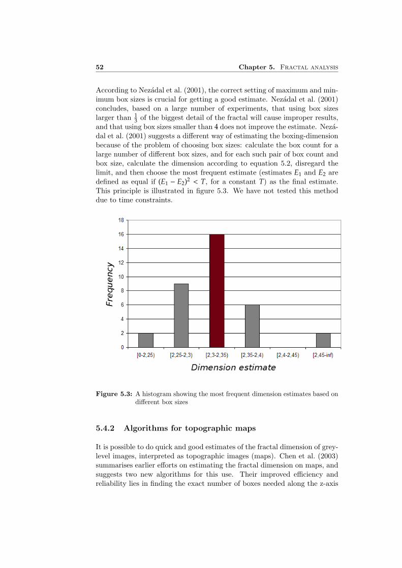
52 Chapter 5. Fractal analysis
According to Nezadal et al. (2001), the correct setting of maximum and min-imum box sizes is crucial for getting a good estimate. Nezadal et al. (2001)concludes, based on a large number of experiments, that using box sizeslarger than 1
3 of the biggest detail of the fractal will cause improper results,and that using box sizes smaller than 4 does not improve the estimate. Neza-dal et al. (2001) suggests a different way of estimating the boxing-dimensionbecause of the problem of choosing box sizes: calculate the box count for alarge number of different box sizes, and for each such pair of box count andbox size, calculate the dimension according to equation 5.2, disregard thelimit, and then choose the most frequent estimate (estimates E1 and E2 aredefined as equal if (E1 − E2)2 < T, for a constant T) as the final estimate.This principle is illustrated in figure 5.3. We have not tested this methoddue to time constraints.
Figure 5.3: A histogram showing the most frequent dimension estimates based ondifferent box sizes
5.4.2 Algorithms for topographic maps
It is possible to do quick and good estimates of the fractal dimension of grey-level images, interpreted as topographic images (maps). Chen et al. (2003)summarises earlier efforts on estimating the fractal dimension on maps, andsuggests two new algorithms for this use. Their improved efficiency andreliability lies in finding the exact number of boxes needed along the z-axis
5.4. Estimating the fractal dimension 53
based on maximum and minimum value of the z-coordinate of pixels incolumns given by a range of x- and y-coordinates.
The simpler of the two algorithms suggested by Chen, the SDBC algorithm,is given below:
s=2 /* s: box size */s_max=M/2 /* s_max: allowable maximum size of box */
while(s <= s_max) dobeginr=s/MN_r(F) = 0for each vertical column of boxes dobeginmin=minimum grey-level valuemax=maximum grey-level valueN_r(F) = CEIL( (max-min+1)/s )
end fors=s+1
end whilecall LINEFIT( log(1/r), log(N_r(F), m, c )dim(F)=m
CEIL is a function that rounds its argument up to the next integer andLINEFIT is a function that returns the least squares regression line basedon its first two arguments and returns the values m and c from the regressionline given as y = mx + c.
These algorithms do not apply to binary images, because in those typesof images, there is not necessarily a single continuous filled area along thez-axis for a given x- and y-coordinate, as for maps. As an illustration ofthis property, consider the map as a terrain and peaks as mountains. Ina topographic map, which is the terrain seen from above, we cannot seeany caves in the mountains, whether caves exist or not. In one or morecross-sections of the terrain, though, caves can be seen if they exist.
5.4.3 Algorithms for binary images
This algorithm applies to one- to three-dimensional binary images.
The basic algorithm for counting boxes that intersects F in a mesh is:
for a number of box sizesfor a number of translationsminCount = INF

54 Chapter 5. Fractal analysis
count = 0for all boxes in meshvisit box.if box intersects F thenincrement count
end forif count < minCount then minCount = count
end forboxcount for this size is minCount
end forDimension is the slope of the regression line forthe points -log(box size), log(boxcount(box size)) for all box sizes.
The basic algorithm has an algorithmic complexity of O(B · T ·N), where Bis the number of different box sizes, T is the number of translations and Nis the number of pixel sites in the image. This is because complete boxesmust be searched in the worst-case to see if F intersects the box or not.
We have come up with some ideas on how to improve this basic algorithm.These ideas are detailed below.
Improvement #1 : Reducing worst-case occurrences. When thereare large empty regions in the image, a hierarchical storage structure likea quadtree or an octree can be used to speed up calculations of boxcountby avoiding search of regions that are known to be empty. Search of emptyregions is the worst-case when visiting boxes to see if the box intersects theobject of interest, because all pixels in the box will have to be visited to besure that the box does not contain the object.
We can use information from the octree (quadtree) to see which regions areworth examining and which are not. To see if a box contains F we canproceed downwards in the octree (quadtree) stopping when we reach a ho-mogeneous region that completely contains the box either counting the boxor not, depending on if the homogeneous region is foreground or background,respectfully. A box can possibly be split over multiple regions in the octree(quadtree). If so, the box should be counted if at least one of these regionsis homogeneous and non-background, traversing the tree to the pixel-level ifnecessary to find out.
Improvement #2 : Doubling of box sizes. In cases where the boxsize reduction factor is 2 it is possible to calculate all box counts in a singlepass of the image. This is because the boxcount for the smallest box sizecan be used to calculate the count for the next-smallest and so on in caseswhere boxes are completely covered by the boxes of next box size.

5.5. Fractal dimension and roughness 55
Note that all numbers that are divisible by two has the property mentionedabove, meaning box count for e.g. box size 5 can be used to calculatethe count for 10, and so on, because boxes of size 5 can be completelycovered by boxes of size 10. Based on this we see that given some boxcounts, i.e. the ones with prime sides, we can quickly calculate their two-multiples, e.g. for sizes 2, 3, 5 we can quickly calculate the count for boxsizes {2, 4, 8, 16, 32, . . .} ∪ {3, 6, 12, 24, 48 . . .} ∪ {5, 10, 20, 40 . . .}.
This improvement can be used simultaneously to improvement #1.
5.4.4 Program code and environment
We have made programs for estimating the fractal dimension on both mapsand binary images, see Appendix A.
5.5 Fractal dimension and roughness
We will here present a small test to see whether the fractal dimension of athree-dimensional surface correlates with perceived roughness of that sur-face.
5.5.1 The test
The surfaces in the test were specified as topographic maps.
A set S of 100 8-bit images of dimension 512 × 512 with intensity value127 was created. Additive Gaussian noise with a mean of 64 and varianceof 25 was added to all images in S. Let’s call the set S with the addednoise for S0. Let Si be S0 with i repetitive Gaussian blurs with the kernel〈0.249, 0.707, 1〉. The surface of one image from S is shown in figure 5.4. Thefractal dimension was estimated for all images in the sets Si|i = 0, 1, 2, 5 bythe plugin for estimating fractal dimension of maps in Appendix A. Theparameters to the plugin was set to “automatic box size”, “end box size” 2and “box reduction factor” 2, with include sub-graph”disabled in all tests.
The results are shown in table 5.1, where d(i) is the average of the dimen-sion estimates of Si and ’Difference’ is the squared difference of the averagedimension estimate of Si and S, (d(S) − d(Si))2. The surfaces of S0 and theblurred images are shown in figure 5.5.

56 Chapter 5. Fractal analysis
Table 5.1: Average of dimension estimates.Measure Dimension estimate Difference N-Variance
d(S) 2.00 0 0d(S0) 2.85 0.72 1.1e − 7d(S1) 2.55 0.30 4.5e − 6d(S2) 2.41 0.17 1.2e − 6d(S5) 2.31 9.6e − 2 1.8e − 6
Figure 5.4: Original topographic image (set S)

5.5. Fractal dimension and roughness 57
(a) Added noise (set S0) (b) Smoothed once (set S1)
(c) Smoothed twice (set S2) (d) Smoothed five times (set S5)
Figure 5.5: Smoothed surfaces

58 Chapter 5. Fractal analysis
5.6 Discussion and future work
The fractal dimension (FD) as a descriptor of surface roughness should becompared to other descriptors of surface roughness both in terms of cor-relation and what they describe. In this respect it might be worthwhileimplementing the SBC algorithm of Chen et al. (2003), which produces thebest known estimates for the FD of topographic maps.
Additionally, the FD of three-dimensional fibrous structures should be ex-amined to see if it correlates with other parameters, both on the microscopicand macroscopic level. We believe that the FD of the skeleton of a fibrousstructure will be a good structural descriptor.
Nezadal et al. (2002) suggests fractal-based methods for evaluating the qual-ity of printed material and printed areas. The method can be used to com-pare the quality of reproduction of the print points, and seems relevant forstudies on reducing the number of missing dots in printouts. It would thusbe interesting to use and extended the method presented by this article.

Chapter 6
Conclusion
Absorption mode images were found to be more suited for analyses thanphase-contrast images.
Techniques for efficient storage and processing of images were suggested.
The most recent method of binarisation of three-dimensional absorptionmode images was explained and commented upon. An improved method ofbinarisation based on a three-dimensional extension of the Susan principleand automatic threshold detection was suggested.
An overview of the current state of feature extraction from porous materialswas presented as well as suggestions for future work in the field. The fractaldimension was judged to be of special interest.
The mathematics behind the fractal dimension and algorithms for determin-ing the fractal dimension of structures were presented.
Programs for three-dimensional Susan filtering and estimating the fractaldimension were developed.
59

60 Chapter 6. Conclusion

Appendix A
Implementation
We have implemented several plugins for the ImageJ environment. Theseplugins are freely available on the Internet, at http://www.pvv.org/~perchrh/imagej.
ImageJ is a public domain Java image processing program inspired by NIHImage for the Macintosh. It runs as an online applet and a downloadableapplication on any computer with a Java 1.1 or later virtual machine. TheImageJ website is http://imagej.sf.net.
A.1 SUSAN plugins
SUSAN means “Smallest Univalue Segment Assimilating Nucleus”. It isa principle introduced by Smith and Brady (1997) that can be used forsmoothing (noise-reduction) and edge detection.
A Susan-smoothing plugin has been implemented. Both 2D (D=dimensional)and 3D smoothing are supported. 2D smoothing is also supported on 3Dimages. A fast-variant of the routine that uses a cubic (or in the 2D case:square) mask of size 3 × 3 × 3 is also supported.
A Susan edge-detection plugin has also been implemented. This plugin hasa fast-option similar to the smoothing plugin.
The implementation is based on code from the FSL1 project. Their codewas made available to ImageJ through the use of the Java Native Interface(JNI). JNI enables the integration of natively compiled code with Java.The native code is placed in a library, and a function is written in Java to
1FMRIB Software Library, written by the Oxford Centre for Functional Magnetic Res-onance Imaging of the Brain, and available at http://www.fmrib.ox.ac.uk/fsl/
61

62 Appendix A. Implementation
convert between the different data representations. JNI facilitates this dataconversion.
The Susan plugins are under the same license as the FSL, due to the sharedcode, which is a free non-commercial licence. For details see http://www.fmrib.ox.ac.uk/fsl/fsl/licence.html.
A.2 Plugins for fractal analysis
Plugins for estimating the fractal dimension of 2D and 3D binary images andof 2D grey-level images interpreted at topographic surfaces (maps) has beenimplemented. They support offsets for added reliability and reproduceabilityof results. The algorithms used is those presented in Chapter 5.
The plugins are licenced under the GNU public licence (GPL), seehttp://www.gnu.org/licenses/gpl.html for details.

Bibliography
Antoine, C., Nygard, P., Holmstad, R., Gregersen, Ø. W., Weitkamp, T., Rau,C., Solheim, O. and Houen, P.-J.: 2001, Binarisation of 3d images of paperobtained by phase-contrast x-ray microtomography, Research techniques fortomorrow’s papermaking, pp. 1–4.
Araonsson, M.: 2002, On 3D Fibre Measurements of digitized paper — from mi-croscopy to fibre network, PhD thesis, Swedish University of Agricultural Sci-ences.
Arns, C., Knackstedt, M., Gregersen, Ø. and Holmstad, R.: 2004, Characterisationof 3d structure and transport properties of paper from tomographic images,The 2004 Progress in Paper Physics Seminar, pp. 64–66.
Arns, C., Pinczweski, W., Knackstedt, M. and Lindquist, W.: 2001, Accurateestimation of transport properties from microtomographic images, GeophysicalResearch Letters 28(17), 3361–3364.
Bajajy, C., Ihmz, I., Minz, J. and Ohz, J.: 2004, Simd optimization of linearexpressions for programmable graphics hardware, Computer Graphics Forum23(8), 1–8.
Brunborg, H. and Smørgrav, T.: 2003, Physically based light simulation using for-ward raytracing, Master’s thesis, Norwegian University of Science and Tech-nology.
Chen, W.-S., Yuan, S.-Y. and Hsieh, C.-M.: 2003, Two algorithms to estimatefractal dimension of gray-level images, Optical Engineering 42(8), 2452–2464.
Cybenko, G.: 1989, Approxmation by superpositions of a sigmoidal function, Math-ematics of Control, Signals and Systems 2(4), 303–314.
Falconer, K.: 2003, Fractal Geometry—Mathematical Foundations and Applica-tions, 2 edn, John Wiley & Sons, Inc.
Garboczi, E., Bentz, D. and Martys, N.: 1999, Digital images and computer mod-elling, Experimental Methods for Porous Media, Academic Press, New York,pp. 1–41.
Gary Chinga, Ø. G. and Dougherty, R.: 2003, Paper surface characterization bylaser profilometry and image analysis, Journal of microscopy and analysis84(4).
63

64 Bibliography
Goel, A., Arns, C., Knackstedt, M., Gregersen, Ø. and Holmstad, R.: 2004, Effectof papermaking variables on the detailed 3d paper structure assessed by x-raymicrotomography, The 2004 Progress in Paper Physics Seminar, pp. 67–69.
Hilpert, M. and Miller, C.: 2001, Pore-morphology based simulation of drainage intotally wetting porous media, Advances in Water Resources 24, 243–255.
Hjelle, G. A.: 2002, Quasidisks—examples and counterexamples, Master’s thesis,the Norwegian University of Science and Technology.
Holen, R. and Hagen, M.: 2003, Pre-processing and segmentation of micro tomo-graphic images of paper. Master-level student project.
Holen, R. and Hagen, M.: 2004, Segmentation on absorption mode x-ray microtomographic images of paper, Master’s thesis, Norwegian University of Scienceand Technology.
Holmstad, R.: 2004, Methods for paper structure characterization by means of imageanalysis, PhD thesis, Norwegian University of Science and Technology.
Holmstad, R., Antonie, C., Nygard, P. and Helle, T.: 2003, Quantification ofthe three-dimensional paper structure: Methods and potential, Pulp & Pa-per Canada 104(7), 186–189.
Huang, S., Goel, A., Ramaswamy, S., Ramarao, B. V. and Choi, D.: 2002, Trans-verse and in-plane pore structure characterization of paper, Appita Journal55(3), 230–234.
ISO4287: 2000, Geometrical product specification (GPS) — Surface texture: Pro-file method – Terms, definitions and surface texture parameters, Internationalstandard: ISO 4287, International Organization for Standardization.
Kaufman, A.: 1994, Voxels as a computational representation of geometry.URL: http: // citeseer. ist. psu. edu/ kaufman94voxels. html
Levoy, M.: 1988, Display of surfaces from volume data, IEEE Comput. Graph.Appl. 8(3), 29–37.
Lin, K. C.: 2003, Fast image thresholding by finding the zero(s) of the first deriva-tive of between-class variance, Mach. Vision Appl. 13(5-6), 254–262.
Lorensen, W. E. and Cline, H. E.: 1987, Marching cubes: A high resolution 3Dsurface construction algorithm, Computer Graphics (SIGGRAPH ’87 Proceed-ings), Vol. 21, pp. 163–169.
Mandelbrot, B.: 1977, Fractals: Form, Chance and Dimension, W.H. Freeman.
Martys, N. and Hagedorn, J.: 2002, Multiscale modeling of fluid transport in hetero-geneous materials using discrete boltzmann methods, Materials and Structures35, 650–649.
Moreland, K. and Angel, E.: 2003, The fft on a gpu, SIGGRAPH/EurographicsWorkshop on Graphics Hardware, pp. 112–119.
Nezadal, M., Zmeskal, O. and Buchnıcek, M.: 2001, The box-counting: Criticalstudy, 4th Conference on Prediction, Synergetic and more..., the Faculty ofManagement, Institute of Information Technologies, Faculty of Technology,Tomas Bata University in Zlin, 18.

Bibliography 65
Nezadal, M., Zmeskal, O., Buchnıcek, M. and Ceppan, M.: 2002, Fractal analysis ofprinted structures, Journal of Imaging Science and Technology 46(5), 453–456.
Oh, W. and Lindquist, B.: 1999, Image thresholding by indicator kriging, PatternAnalysis and Machine Intelligence, IEEE Transactions on 21, 590–602.
Peel, J. D.: 1999, Paper science and paper manufacture, Angus Wilde PublicationsInc.
Pentland, A.: 1984, Fractal-based description of natural scenes, IEEE transactionson Pattern Analysis and Machine Intelligence 6(6), 661–674.
Ramaswamy, S., Huang, S., Goal, A., Cooper, A., Choi, D., Badyopadhyay, A. andRamarao, B.: 2001, The 3d structure of paper and its relationship to moisturetransport in liquid and vapor forms, The science of paper making, pp. 1289–1311, 1641–1650. Transactions of the 12th fundamental research symposium.Vol. 2&3.
Samet, H. and Webber, R.: 1988, Hierarchical data structures and algorithmsfor computer graphics. i. fundamentals, Computer Graphics and Applications,IEEE 8(3), 48–68.
Sarkar, N. and Chaudhuri, B.: 1992, An efficient approach to estimate fractaldimension of textural images, Pattern Recognition 29(6), 1035–1041.
Skocir, P., Marusic, B. and Tasic, J.: 2002, A three-dimensional extension of thesusan filter for wavelet video coding artifact removal, 11th Mediterranean Elec-trotechnical Conference, pp. 395–398.
Smith, J. T., Lange, G. and Marks, W.: 1996, Fractal methods and results incellular morphology — dimensions, lacunarity and multifractals, Neurosciencemethods 69, 123–136.
Smith, S. and Brady, J.: 1997, SUSAN - a new approach to low level image pro-cessing, Int. Journal of Computer Vision 23(1), 45–78.
Sonka, M., Hlavac, V. and Boyle, R.: 1999, Image Processing, Analysis, and Ma-chine Vision, 2. edn, Thomson Publishing inc.
Stoen, T.: 2003, Evaluering av ruhet pa trykte papiroverflater og dens innvirkningpa trykkvalitet, Master’s thesis, Norwegian University of Science and Technol-ogy. Title in English is ”An evaluation of paper surface roughness for printedpaper and its effect on print quality.
Wang, L., Ramaswamy, S. and Ramarao, B.: 2004, Surface structure characteriza-tion of porous materials using x-ray micro computed tomography, The 2004Progress in Paper Physics Seminar, pp. 54–62.
Wilson, D., Jabri, K. and Aufrichtig, R.: 1999, Perception of temporally filtered x-ray fluoroscopy images, Medical Imaging, IEEE Transactions on 18(1), 22–31.
Yang, H.: 2001, A geometric and Statistical Analysis of Fibrous Materials fromThree-Dimensional High Resolution Images, PhD thesis, State University ofNew York.

Index
anisotropic, 7
background, 25binarisation, 13, 19binary, 7bits, 12byte, 12
caching, 12calendering, 44Cropping, 20
ESRF, 4
Fast-Susan, 27flood-fill algorithm, 22foreground, 25fractal, 47fractal dimension, 47FSL, 61
gigabyte (GB), 12
headbox, 44
information-preserving, 13iso-valued, 10isotropic, 7
Java, 17
kilobyte (KB), 12
lumen, 40
Marching Cubes algorithm, 10medial axis transform, 39megabyte (MB), 12modulo, 15
N-adjacent, 9N-connected, 9
octree, 13
paging, 14PFI, 1pixels, 8polygons, 10pore throats, 39porous phase, 19
ray casting, 11
segmentation, 13skeleton, 39structure anisotropy, 35surface fitting, 10surface rendering techniques, 9SUSAN, 21synchrotron, 3
Thresholding, 21topological dimension, 47
volume rendering techniques, 10voxels, 8
X-ray micro tomography, 2X-ray tomography, 2
zero order interpolation, 8
66