measurements of volatile organic compounds at a suburban ground

Atmos. Chem. Phys., 11, 2399–2421, 2011www.atmos-chem-phys.net/11/2399/2011/doi:10.5194/acp-11-2399-2011© Author(s) 2011. CC Attribution 3.0 License.

AtmosphericChemistry

and Physics

Measurements of volatile organic compounds at a suburban groundsite (T1) in Mexico City during the MILAGRO 2006 campaign:measurement comparison, emission ratios, and source attribution

D. M. Bon1,2,3, I. M.Ulbrich 2,3, J. A. de Gouw1,2, C. Warneke1,2, W. C. Kuster1, M. L. Alexander4, A. Baker5,A. J. Beyersdorf5,*, D. Blake5, R. Fall2,3, J. L. Jimenez2,3, S. C. Herndon6, L. G. Huey7, W. B. Knighton8, J. Ortega4,** ,S. Springston9, and O. Vargas7

1NOAA Earth System Research Laboratory, Boulder, Colorado, USA2Cooperative Institute for Research in Environmental Sciences, University of Colorado, Boulder, Colorado, USA3Department of Chemistry and Biochemistry, University of Colorado, Boulder, Colorado, USA4Pacific Northwest National Laboratory, Richland, Washington, USA5University of California, Irvine, California, USA6Aerodyne Research Inc. Billerca, Massachusetts, USA7Georgia Institute of Technology, Atlanta, Georgia, USA8Montana State University, Bozeman, Montana, USA9Brookhaven National Laboratory, Upton, New York, USA* now at: NASA Langley Research Center, Hampton, Virginia, USA** now at: National Center for Atmospheric Research, Atmospheric Chemistry Division, Boulder, Colorado, USA

Received: 15 September 2010 – Published in Atmos. Chem. Phys. Discuss.: 8 October 2010Revised: 28 February 2011 – Accepted: 8 March 2011 – Published: 16 March 2011

Abstract. Volatile organic compound (VOC) mixing ra-tios were measured with two different instruments at the T1ground site in Mexico City during the Megacity Initiative:Local and Global Research Observations (MILAGRO) cam-paign in March of 2006. A gas chromatograph with flameionization detector (GC-FID) quantified 18 light alkanes,alkenes and acetylene while a proton-transfer-reaction ion-trap mass spectrometer (PIT-MS) quantified 12 VOC speciesincluding oxygenated VOCs (OVOCs) and aromatics. A GCseparation system was used in conjunction with the PIT-MS(GC-PIT-MS) to evaluate PIT-MS measurements and to aidin the identification of unknown VOCs. The VOC measure-ments are also compared to simultaneous canister samplesand to two independent proton-transfer-reaction mass spec-trometers (PTR-MS) deployed on a mobile and an airborneplatform during MILAGRO. VOC diurnal cycles demon-strate the large influence of vehicle traffic and liquid propanegas (LPG) emissions during the night and photochemicalprocessing during the afternoon. Emission ratios for VOCsand OVOCs relative to CO are derived from early-morning

Correspondence to:J. A. de Gouw([email protected])

measurements. Average emission ratios for non-oxygenatedspecies relative to CO are on average a factor of∼2 higherthan measured for US cities. Emission ratios for OVOCs areestimated and compared to literature values the northeast-ern US and to tunnel studies in California. Positive matrixfactorization analysis (PMF) is used to provide insight intoVOC sources and processing. Three PMF factors were dis-tinguished by the analysis including the emissions from ve-hicles, the use of liquid propane gas and the production ofsecondary VOCs + long-lived species. Emission ratios to COcalculated from the results of PMF analysis are compared toemission ratios calculated directly from measurements. Thetotal PIT-MS signal is summed to estimate the fraction ofidentified versus unidentified VOC species.

1 Introduction

Recent estimates of the global emission of volatile organiccompounds (VOCs) into the atmosphere range from about1200 to 1600 TgC yr−1 (Olivier et al., 2005; Goldstein andGalbally, 2007; Reimann and Lewis, 2007; Williams andKoppmann, 2007; Yokelson et al., 2008). Major sourcesof atmospheric VOCs include vegetative emission, biomass

Published by Copernicus Publications on behalf of the European Geosciences Union.

http://creativecommons.org/licenses/by/3.0/

2400 D. M. Bon et al.: Measurements of volatile organic compounds at a suburban ground site

burning, and the use of fossil fuels. On a global scale, VOCemissions are dominated by isoprene, which accounts forabout 65% of biogenic emissions and 40% of total VOCemissions (Guenther et al., 1995, 2006; Williams and Kopp-mann, 2007). Biomass burning, both natural and as the re-sult of human activity, and fossil fuel use are each thought toaccount for about 10% of global VOC emissions (Reimannand Lewis, 2007). Recent estimates suggest the contribu-tion from biomass burning could be as large as 500 TgC yr−1

(Yokelson et al., 2008). Regardless of global emissions, anyof these sources can dominate locally and regionally. An-thropogenic VOC emissions often dominate in areas of highpopulation density and contribute significantly to urban airpollution (Olivier et al., 2005; Reimann and Lewis, 2007).Air pollution is of growing international concern and con-tributes to approximately 2 million premature deaths per yearworldwide (World Health Organization, 2008).

In and around heavily populated urban areas, VOCs re-leased as a result of fossil fuel use are significant contrib-utors to the formation of photochemical smog and ground-level ozone. Ozone, a secondary pollutant that is formed byphotochemical reactions involving VOCs and nitrogen ox-ides (NOx), has direct adverse effects on human health andcan damage agricultural crops (Finlayson-Pitts, 1997; Krupaet al., 2001). Urban VOCs can also contribute to formation ofparticulate pollution that has significant detrimental effectson human health (Brunekreef and Forsberg, 2005; van Zelmet al., 2008). VOCs and particulate emissions related to hu-man activity and the subsequent formation of secondary or-ganic aerosol (SOA) have the potential to affect climate (Ra-manathan et al., 2007). Mechanisms of SOA formation fromurban VOCs are not well understood (de Gouw et al., 2005;Volkamer et al., 2006; Hallquist et al., 2009).

The Mexico City Metropolitan Area (MCMA), a high-altitude sub-tropical megacity with a population of about18 million people, is an urban center where a dense popula-tion and a local geography that restricts transport, contributeto the city’s significant air quality problems. Hydrocarbonmeasurements in 1993, 2002, and 2003 showed highly el-evated levels of many anthropogenic VOCs within the city(Blake and Rowland, 1995; Rogers et al., 2006; Velasco etal., 2007). The MILAGRO campaign (Megacity Initiative:Local and Global Research Observations) in March 2006was designed to address the impact of these emissions ona variety of scales from local to global, and builds on resultsfrom smaller multi-investigator campaigns such as IMADA-AVER and MCMA-2003 (Edgerton et al., 1999; Molina etal., 2007, 2010).

During MILAGRO a variety of different instruments andtechniques were used to quantify VOCs from both fixed sitesand mobile platforms (Heald et al., 2008; Apel et al., 2010).VOC measurements were made by two different ground-based instruments at the sub-urban T1 site (Fast et al., 2007):an in-situ gas chromatograph with flame ionization detec-tion (GC-FID) was used to measure light hydrocarbons and

a proton-transfer-reaction ion-trap mass spectrometer (PIT-MS) was used to measure acetonitrile, aromatics and oxy-genated VOCs (de Gouw et al., 2009). Here, these mea-surements are compared with canister sample analyses andwith proton-transfer-reaction mass spectrometry (PTR-MS)measurements made from the Aerodyne mobile laboratoryand from the US Department of Energy G1 aircraft. Be-cause the Aerodyne mobile laboratory and the G1 aircraftalso sampled near other surface sites and because canistersamples were collected at many surface sites and from theNASA DC-8 and NCAR C-130 aircraft, these comparisonscan be used to evaluate the consistency of VOC data obtainedthroughout the campaign (Kleinman et al., 2008; Fortner etal., 2009; Karl et al., 2009; Apel et al., 2010). In addition,this study supplements our understanding of the specificity ofproton-transfer-reaction mass spectrometry (PTR-MS) mea-surements in a dense megacity with a complex VOC compo-sition that challenges the analytical capabilities of this tech-nique (de Gouw and Warneke, 2007).

Diurnal cycles of most VOCs at T1 were pronounced witha high peak in the morning when emissions accumulated ina shallow mixing layer (de Gouw et al., 2009). A similardiurnal pattern was observed during the MCMA-2003 studyand at the T0 ground site during the MILAGRO campaign(Velasco et al., 2007; Fortner et al., 2009). The T1 data areused here to determine urban emission ratios versus CO, andthese are compared to those from previous studies in the US(Warneke et al., 2007; Baker et al., 2008; Ban-Weiss et al.,2008). The effects of chemical removal and production ofVOCs were pronounced in the afternoon and are discussedelsewhere in more detail (de Gouw et al., 2009).

Positive Matrix Factorization (PMF), a factorizationmodel widely used for environmental source apportionment(Paatero and Tapper, 1994; Ulbrich et al., 2009) is appliedhere to the VOC data collected at T1 during the campaign.PMF and other similar factorization methods (e.g. PrincipalComponent Analysis) have been applied previously for VOCmeasurements at urban ground sites where VOCs have dis-tinct sources or diurnal profiles (Harley et al., 1992; Buzcuand Fraser, 2006; Millet et al., 2006; Legreid et al., 2007;Song et al., 2007). We use the results from the PMF analy-sis to estimate emission ratios and compare these with emis-sion ratios derived directly from ground-based VOC mea-surements.

2 Methods

2.1 VOC measurements at T1

The T1 ground site (19◦42′11′′N, 98◦58′55′′W) was located30 km to the northeast of Mexico City on the campus ofthe Universidad Tecnologica de Tecamac (UTTEC). VOCmeasurements at the site were made using (1) a custom-built proton-transfer ion-trap mass spectrometer (PIT-MS),

Atmos. Chem. Phys., 11, 2399–2421, 2011 www.atmos-chem-phys.net/11/2399/2011/

D. M. Bon et al.: Measurements of volatile organic compounds at a suburban ground site 2401

35

982 Figure 1. Sampling periods for the VOC measurement methods and CO at the T1 ground site in 983

Mexico City during the MILAGRO campaign. Approximate daylight hours (7:00 AM – 19:00 PM 984

local time) are shown in yellow. 985

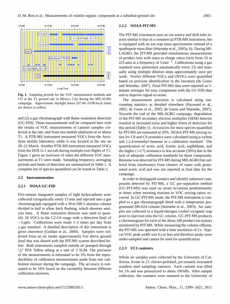
Fig. 1. Sampling periods for the VOC measurement methods andCO at the T1 ground site in Mexico City during the MILAGROcampaign. Approximate daylight hours (07:00–19:00 local time)are shown in yellow.

and (2) a gas chromatograph with flame ionization detection(GC-FID). These measurements will be compared here withthe results of VOC measurements of canister samples col-lected at the site, and from two mobile platforms at or aboveT1. A PTR-MS instrument measured VOCs from the Aero-dyne mobile laboratory while it was located at the site on20–21 March. Another PTR-MS instrument measured VOCsfrom the DOE G-1 aircraft during multiple over flights of T1.Figure 1 gives an overview of when the different VOC mea-surements at T1 were made. Sampling frequency, averagingperiods and limits of detection are summarized in Table 1. Acomplete list of species quantified can be found in Table 2.

2.2 Instrumentation

2.2.1 NOAA GC-FID

Five-minute integrated samples of light hydrocarbons werecollected cryogenically every 15 min and injected into a gaschromatograph equipped with a 50 m DB-5 alumina columndivided in half to allow back flushing, which shortens anal-ysis time. A flame ionization detector was used to quan-tify 18 VOCs in the C2-C6 range with a detection limit of∼5 pptv. Calibrations were made 1–2 times per day froma gas standard. A detailed description of this instrument isgiven elsewhere (Goldan et al., 2000). Samples were col-lected from an air intake approximately 6 m above groundlevel that was shared with the PIT-MS system described be-low. Both instruments sampled outside air pumped through1/4” PFA Teflon tubing at a rate of 3 SLM. The precisionof the measurements is estimated to be 5% from the repro-ducibility of calibration measurements made from one cali-bration mixture during the campaign. The accuracy is esti-mated to be 10% based on the variability between differentcalibration mixtures.

2.2.2 NOAA PIT-MS

The PIT-MS instrument uses an ion source and drift-tube re-actor similar to that of a commercial PTR-MS instrument, butis equipped with an ion trap mass spectrometer instead of aquadrupole mass filter (Warneke et al., 2005a, b). During MI-LAGRO, the PIT-MS provided simultaneous measurementsof product ions with mass to charge ratios (m/z) from 33 to225 amu at a frequency of 5 min−1. Calibrations using a gasstandard were performed automatically every 2 h and man-ually using multiple dilution steps approximately once perweek. Twelve different VOCs and OVOCs were quantifiedbased on previous identification in the literature (de Gouwand Warneke, 2007). Final PIT-MS data were reported as 5-minute averages for easy comparison with the GC-FID dataand to improve signal-to-noise.

The measurement precision is calculated using ion-counting statistics as detailed elsewhere (Hayward et al.,2002; de Gouw et al., 2003; de Gouw and Warneke, 2007).Towards the end of the MILAGRO campaign, degradationof the PIT-MS secondary electron multiplier (SEM) detectorresulted in increased noise and higher limits of detection forthis period (Table 1). Accuracies for most species quantifiedby PIT-MS are estimated at 20%. NOAA PIT-MS mixing ra-tios for C8 and C9 aromatics were calculated using p-xyleneand 1,2,4-trimethyl benzene in a calibration standard. Thequantification of acetic acid, formic acid, naphthlane, andthe higher (>C7) aromatics is less accurate (50%) due to thelack of adequate calibration standards for these compounds.Benzene was detected by PIT-MS during MILAGRO but suf-fered from interference from clusters of water with proto-nated acetic acid and was not reported in final data for thecampaign.

In order to distinguish isomers and identify unknown com-pounds detected by PIT-MS, a GC pre-separation method(GC-PIT-MS) was used on seven occasions predominantlyat times when morning maxima in VOC mixing ratios oc-curred. In GC-PIT-MS mode, the PIT-MS instrument is cou-pled to a gas chromatograph fitted with a temperature pro-grammed DB-624 column (Warneke et al., 2003). Air sam-ples are collected in a liquid-nitrogen cooled cryogenic trapprior to injection onto the GC column. GC-PIT-MS producesa chromatogram for each of the about 180 product ion massesmonitored by PIT-MS. While measuring the column effluent,the PIT-MS was operated with a time resolution of 2 s. Typi-cal VOC peak width was 4 s or less and therefore peaks wereunder-sampled and cannot be used for quantification.

2.2.3 UCI canisters

Whole air samples were collected by the University of Cal-ifornia, Irvine in 2 L electro-polished, pre-treated, evacuatedstainless steel sampling canisters. Each canister was filledfor 3 h and was pressurized to about 100 kPa. After samplecollection, the canisters were returned to the University of

www.atmos-chem-phys.net/11/2399/2011/ Atmos. Chem. Phys., 11, 2399–2421, 2011


Table 1. Limits of detection for individual VOCs quantified during the MILAGRO campaign by PIT-MS and PTR-MS.

Instrument: NOAA PIT-MS Aerodyne PTR-MS DOE PTR-MSperiod: 5 min 1σ 1σ

date: 11–27 Mar 28–31 Mar∗

Compound Limit of Detection (pptv)

toluene 150 (800) 110 1006C8 aromatics 100 (800) 200 1106C9 aromatics 100 (800) 160 110

6C10 aromatics 100 (800)6C11 aromatics 100 (800)

naphthalene 100 (800)

methanol 1500 (1500) 530acetaldehyde 300 (1500) 400 350

acetone 150 (800) 230 250acetic acid 300 (1200) 350

methyl ethyl ketone 300 (2000) 150

acetonitrile 100 (800) 85

∗ PIT-MS LODs reported for two periods 11–27 March and 28–31 March . LOD changed due to hardware problems.

California, Irvine, where they were analyzed for CH4, CO,hydrocarbons, halocarbons and alkyl nitrates. Detection lim-its for all species compared here were less than 3 pptv withprecisions between 1% and 4%. For more detailed descrip-tions of the UCI measurements we refer to (Colman et al.,2001). Canister samples were also collected at the T0 groundsite and onboard the NASA DC-8 and NCAR C-130 aircraft,and analyzed using the same methodology.

2.2.4 Aerodyne PTR-MS

A commercial PTR-MS (Ionicon Analytik, Austria) instru-ment was deployed on the Aerodyne mobile laboratory dur-ing the campaign (Rogers et al., 2006; Herndon et al., 2008).The mobile laboratory was parked at the T1 site for ap-proximately 40 h from 04:00 UTC on 20 March 2006 until18:00 UTC on 21 March 2006. Calibrations were made atregular intervals using a gas calibration standard and averagecalibration factors were applied to the data after the cam-paign. Two scan modes were used for the mobile laboratoryPTR-MS. In the first mode, 24 scans of 9 masses were madeeach with a one second dwell time. This was followed by 12cycles of the full mass range (20–160 amu) with a 0.1 s dwelltime. The data obtained in both modes were averaged on a1-min time basis for comparison to PIT-MS measurementsduring this period.

2.2.5 DOE PTR-MS

The Pacific Northwest National Laboratory deployed a com-mercial PTR-MS on the DOE G1 aircraft. Eleven VOCswere measured with a frequency of 0.1 s−1. PTR-MS dwell

times on the aircraft ranged from 0.5–1.0 s per mass and cal-ibrations were typically done at least twice per flight day.Thirty-eight over-flights of T1 occurred during MILAGRO.

2.2.6 Carbon monoxide measurements

Carbon monoxide measurements were made at the T1 groundsite by the Georgia Institute of Technology using a modi-fied Thermo Electron 48C CO monitor (Parrish et al., 1994).CO measurements were reported on a 1-minute time base.The precision and accuracy of these data are estimated to be±5 ppbv and±5%, respectively.

CO was also quantified by gas chromatography from theUC Irvine canisters. These measurements agreed with the in-situ measurements averaged over the canister sampling peri-ods to within 5% (r2

= 0.90).

2.3 Positive Matrix Factorization (PMF)

2.3.1 PMF method

The PMF algorithm solves the bilinear, receptor-only, un-mixing model, with positively-constrained factor values,and has been widely used for factor analysis and source-apportionment of both particulate matter and VOC measure-ments (Zhao et al., 2004; Brown et al., 2007; Engel-Cox andWeber, 2007; Reff et al., 2007; Lanz et al., 2008; Ulbrich etal., 2009; Slowik et al., 2010). Some concepts that are rele-vant to the understanding of this work are briefly describedhere. For additional details about the method, the reader isreferred to the above references.

For PMF analysis, data are assembled into a 2 dimensionalm× n matrix X such that each of thei rows contains the



Table 2. Slopes resulting from ODR regression of scatter plots be-tween VOCs measured by 2 or more techniques during MILAGRO.Also shown here are 1σ uncertainties in slopes, correlation(r2) co-efficients, and the number of points compared(N).

best fit slope r2 N

NOAA GC-FID:UCI canisters

propane 0.98± 0.04 0.96 128n-butane 1.02± 0.03 0.97 128i-butane 1.02± 0.03 0.97 128n-pentane 1.04± 0.03 0.98 128i-pentane 0.89± 0.02 0.98 128n-hexane 0.94± 0.03 0.97 128ethylene 0.90± 0.03 0.97 129propylene 1.00± 0.03 0.97 1281-butene + 2-methyl propene 0.99± 0.04 0.96 128cis-2-butene 0.95± 0.04 0.95 128trans-2-butene 0.79± 0.03 0.96 1281-pentene 1.18± 0.16 0.87 71cis-2-pentene 1.00± 0.06 0.94 77trans-2-pentene 1.03± 0.04 0.96 982-methy 2-butene 0.78± 0.07 0.90 603-methy 1-butene 0.93± 0.12 0.87 82acetylene 0.74± 0.04 0.94 129

NOAA PIT-MS:UCI canisters

toluene 1.07± 1.74 0.87 1126C8 aromatics 3.38± 0.14 0.87 1086C9 aromatics 2.68± 0.44 0.72 101

NOAA PIT-MS:Aerodyne PTR-MS

methanol 0.68± 0.11 0.84 1605acetaldehyde 1.10± 0.21 0.81 1695acetone 1.00± 0.14 0.86 1695toluene 1.61± 0.18 0.89 16856C8 aromatics 1.39± 0.18 0.87 16856C9 aromatics 1.38± 0.22 0.84 1685

NOAA PIT-MS:DOE G1 PTR-MS

acetonitrile 0.93± 0.17 0.06 15acetaldehyde 0.97± 0.13 0.18 15acetone 0.86± 0.07 0.50 15acetic acid 0.50± 0.08 0.10 15methyl ethyl ketone 0.84± 0.09 0.36 15toluene 1.07± 0.14 0.51 156C8 aromatics 0.88± 0.17 0.04 156C9 aromatics 0.30± 0.14 0.23 9

measured VOC mixing ratios at sampling timeti and each ofthej columns contains the time series of a sampled VOCj . Acorresponding matrix is assembled specifying the measure-ment precision (“uncertainty”) for each point in the data ma-trix (σij ). The bilinear unmixing model represents the mea-

sured VOC concentrations as the sum of the contributions ofp factors, each of which is comprised of a chemical profile(f ) and a factor time series (g), such that for each point inthe data matrix (Xij ):

Xij =

∑p

gipfpj +eij (1)

whereeij is the fit residual for each matrix (Paatero and Tap-per, 1994; Paatero, 1997; Ulbrich et al., 2009).

The PMF algorithm finds solutions of the model by mini-mizing a “quality of fit” parameterQ defined as:

Q =

m∑i=1

n∑j=1

(eij/σij

)2

. (2)

The minimum expected value ofQ/(Qexp) is obtained whenall data elements have been fit within their uncertainty (i.e.,eij /σ ij ∼ 1), thusQexp should be approximatelym×n forlarge datasets.Q values can be normalized toQexp, such thatthe expected best fit would haveQ/Qexp∼ 1. The numberof factors that best represent the dataset is ultimately chosenby the user, commonly based on both (1) quantities such asQ/Qexp that characterize the quality of the reconstruction,and (2) the physical plausibility of the factors. PMF solutionsfor a given number of factors are not mathematically unique,i.e. linear transformations (“rotations”) of the factor time se-ries and source profiles may result in a acceptable fit to thedata with similar but slight larger values ofQ (Paatero andHopke, 2009). A subset of approximate linear transforma-tions can be explored in PMF using the FPEAK parameter.

In this study, we use the PMF2 algorithm in robust modewith default convergence and outlier criteria values. We eval-uate the analysis using the recently-developed PMF Evalua-tion Tool (PET) (Ulbrich et al., 2009).

2.3.2 Data preparation

PIT-MS measurements were averaged over GC-FID sam-pling periods (Fig. 1, Table 1) for the period from 11–27 March 2006. Periods when either instrument was offline were excluded from the PMF analysis. The data ma-trix for the analysis presented here consisted of 851 simul-taneous measurements (rows) from the GC-FID and PIT-MSinstruments, arranged so that 18 columns contain the time se-ries of 18 species from the GC-FID, 12 columns contain thetime series of 12 VOCs quantified by PIT-MS, and the final35 columns contain the time series of 35 PIT-MS ion signalsnot quantified (65 columns total). The 35 PIT-MS ion signalschosen were not identified as specific molecules, but all didshow a significant signal during the campaign.

For the GC-FID data we used 5 pptv or 5%, whichevernumber was larger, to calculate errors for PMF analysis. Er-rors for the PIT-MS data were calculated using ion countingstatistics (de Gouw and Warneke, 2007). The error for 11PIT-MS masses with signal to noise ratios (SNR) less than



2 was increased by a factor of 4, as is typical for the PMFmethod (Paatero and Hopke, 2003; Ulbrich et al., 2009).None of the measurements considered in the analysis had aSNR <1. Error was increased for only one quantified PIT-MS mass (m/z129, naphthalene). Results of PMF analysisand an estimate of the uncertainties involved in this analysisare discussed in Sect. 4.

3 Data quality evaluation

The quality of VOC data obtained at T1 was evaluated us-ing direct measurement comparisons between the two NOAAmeasurements and other measurements where possible. Theselectivity of the PIT-MS data was evaluated using GC-PIT-MS analyses.

3.1 Measurement comparisons

3.1.1 NOAA GC-FID versus UCI canisters

The on-line GC-FID measurements were compared to UCIcanister measurements for 17 compounds. For the purpose ofthese comparisons, the on-line GC-FID data were averagedover the 3-hour sampling times of the UCI canisters. Exam-ples are shown for propane, ethylene and acetylene (Fig. 2a–c). The data in Fig. 2 were fit using 2-sided, orthogonaldistance regressions (ODR). The resulting regression slopes(s), and values of the linear correlation coefficient (r2) aresummarized in Table 2 for all 17 overlapping VOC measure-ments. For all VOCs, the degree of correlation between thein-situ and canister measurements was high (r2 > 0.87) andmost measurements agreed within the 10% accuracy of thein-situ measurements. Notably, the canister measurementsof acetylene (Fig. 2c) were systematically higher than thosemade in-situ. The reasons for this difference are unknown;calibration standards were not compared for the purpose ofthis study. Our GC measurements in the Arctic in 2008 weresystematically higher than canister samples analyzed by theNOAA Global Monitoring Division (Gilman, et al., 2010).As reported in previous work (Apel et al., 1994), it appearsthat the accuracy of the measurement of acetylene is consid-erably outside the 10% calibration uncertainty estimated forother species. Further work is needed to resolve the consid-erable calibration discrepancies for this important species.

3.1.2 NOAA PIT-MS versus UCI canisters

Both the PIT-MS and the UCI canisters reported mixing ra-tios for aromatic compounds. An example of the compar-isons is shown for toluene in Fig. 2d. The PIT-MS data wereaveraged onto the canister sampling times for the purpose ofthis plot. The two measurements correlated well and agreedquantitatively within 7%. The other PIT-MS measurementsof aromatics correlated well but were systematically higherthan the UCI canister measurements (Table 2). The reasons

for these differences are unknown; calibration standards werenot compared for the purpose of this study.

PTR-MS measurements of higher aromatics represent thesums of many different isomers, each with its own calibra-tion uncertainty. As a result, inter-comparisons tend to showlarger differences than for single compounds (de Gouw andWarneke, 2007). For example, out of 5 published compar-isons of C8 aromatic measurements, three studies comparedwithin 20% and two showed differences of factors of 2 and3. The GC-PIT-MS results presented later in this sectionshow no significant interferences on masses associated witharomatic compounds that might explain these discrepancies.Previous work in the US also shows no evidence of interfer-ence on these masses (Warneke et al., 2003). We concludethat calibration uncertainties appear to be the most likely ex-planation for measurement disagreements.

3.1.3 NOAA PIT-MS vs. Aerodyne PTR-MS

The Aerodyne mobile laboratory collected data at the T1 sitefor two days during the campaign (Fig. 1). Six VOCs weremeasured by both the NOAA PIT-MS and the Aerodyne mo-bile laboratory PTR-MS. Figure 2e shows the measurementcomparison for acetaldehyde. Slopes and correlation coeffi-cients for all 6 VOC comparisons are summarized in Table 2.Correlation coefficients (r2) for all 6 compared compoundswere greater than 0.80.

The calibration standards used by both instruments werecompared in the field during MILAGRO. PIT-MS measure-ments of methanol were systematically 32% lower than thoseof the Aerodyne PTR-MS. This difference is similar to thedifference observed (35%) between the calibration standardsused with each of the two instruments. The PIT-MS measure-ments of reported aromatics were systematically 40–60%higher than the Aerodyne PTR-MS measurements (Table 2)but are within the combined measurement uncertainties. Un-like methanol, differences in calibration standards did not ex-plain differences between measurements of aromatics.

3.1.4 NOAA PIT-MS vs. DOE PTR-MS

The DOE G1 aircraft flew over the T1 ground site 38 timesduring MILAGRO. All overpasses occurred in mid-afternoonwhen VOC mixing ratios for primary species were at ornear daily minima. Aircraft overpass altitudes ranged be-tween 800–2800 m above ground level with typical well-mixed daytime boundary layer depths of at least 2000 m.Measurements of boundary layer heights indicate that over-passes of T1 occurred within the boundary layer (Shaw et al.,2007; Fast et al., 2009).

Eight VOC measurements were compared for the 15 over-passes when both instruments were operating. Overpasseswere defined as measurements made by the DOE-G1 instru-ment within a horizontal distance of 5 km from the groundsite. DOE-G1 PTR-MS measurements for each VOC during



36

986 Figure 2. Selected results of the comparison of VOC measurements at the T1 site during MILAGRO. 987

Panels a-c compare the measurements of the NOAA GC-FID and the UC Irvine canister 988

measurements for the same compound. Panel d-f compare measurements made by the NOAA PIT-989

MS to made from the UC Irvine Canisters and by the PTR-MS instruments on the Aerodyne Mobile 990

Laboratory and the DOE G1 aircraft, respectively. Slopes from linear regressions (s) and correlation 991

coefficients, r2, for comparisons are tabulated in Table 2. 992

Fig. 2. Selected results of the comparison of VOC measurements at the T1 site during MILAGRO. Panels(a–c)compare the measurementsof the NOAA GC-FID and the UC Irvine canister measurements for the same compound. Panel(d–f) compare measurements made by theNOAA PIT-MS to made from the UC Irvine Ccanisters and by the PTR-MS instruments on the Aerodyne Mobile Laboratory and the DOEG1 aircraft, respectively. Slopes from linear regressions(s) and correlation coefficients,r2, for comparisons are tabulated in Table 2.

a particular over flight were averaged and compared to PIT-MS ground measurements averaged within a window of±10 min from the over flight period. An example of thecomparison between surface and airborne measurements isshown in Fig. 2f for acetone. Due to the low number of datapoints, linear least-squares fits of the data were constrainedto an intercept of zero for these comparisons. Slopes andr2 values for fits are shown for all 8 VOCs in Table 2. Theinter-comparison is challenging due to: (1) low VOC mixingratios in a narrow concentration range, (2) the large verticalseparation, and (3) short duration of the over-flights. There-fore, correlation coefficients for individual VOCs were low(r2 < 0.55), but most species except the C9-aromatics didnot show large systematic differences between the two mea-surements. Calibration standards were not compared duringthis study.

3.2 GC-PIT-MS

The NOAA PIT-MS was operated in GC-PIT-MS modeseven times during MILAGRO to identify VOCs and evalu-ate PIT-MS measurements at T1. The GC-interface was sim-ilar to that used in a previous study (Warneke et al., 2003);however, the present application is unique in the sense that a

chromatogram is obtained at each detection mass of the PIT-MS. Most GC-PIT-MS analyses occurred early in the daycoincident with peak VOC concentrations. Figures 3 and 4show selected chromatograms from the use of this methodfor PIT-MS signal attribution. Individual masses of interestare discussed in the following section.

The chromatographic peaks observed at masses 33(methanol), 45 (acetaldehyde), 59 (acetone), 93 (toluene),107 (C8-aromatics), and 121 amu (C9-aromatics) were verysimilar to the results from previous GC-PTR-MS measure-ments in urban air (Warneke et al., 2003; de Gouw andWarneke, 2007) and provided no evidence of important in-terferences for any of these compounds.

Acetonitrile is measured by PIT-MS at 42 amu. Interfer-ences from the reaction of alkanes and alkenes with O+

2 ionshave previously been observed using GC-PTR-MS (de Gouwet al., 2003; de Gouw and Warneke, 2007). Interferencesfrom propane were evident in GC-PIT-MS chromatogramsfrom Mexico City where mixing ratios of propane reachedas high as 250 ppbv. From the GC-PIT-MS measurements itis difficult to quantify the sensitivity of the signal at mass42 amu to propane. However, scatter plots of the signalat 42 amu versus propane showed no correlation betweenthe two measurements. We conclude that while propane



37

993 Figure . Select GC-PIT-MS chromatograms obtained during the MILAGRO campaign. Signals 994

reported are sums of six individual chromatograms. The retention time scale is slightly adjusted to be 995 Fig. 3. Select GC-PIT-MS chromatograms obtained during the MI-LAGRO campaign. Signals reported are sums of six individualchromatograms. The retention time scale is slightly adjusted to becomparable with previously reported values for GC-PTR-MS usingthe same GC instrument and temperature program (Warneke et al.,2003).

contributed to the signal at 42 amu, most of the variabilityin the 42 amu signal was due to acetonitrile.

Even masses are typically associated with nitrogen-containing compounds in PTR-MS measurements. The chro-matogram at 54 amu contained a small peak that is at-tributed here to acrylonitrile. However, a larger fraction ofthe signal at 54 amu in on-line measurements comes fromH3O+(H2O)2 clusters at 55 amu; water cluster ions show atail towards lower masses in PIT-MS. Two unidentified even-mass compounds were detected at 46 and 62 amu by GC-PIT-MS but no conclusive identification was established. Lowmixing ratios and isotopic interferences at adjacent massesfrom more abundant compounds (acetaldehyde and aceticacid respectively) prevent even tentative quantification ofthese even mass compounds.

Formic acid has previously been reported as the domi-nant contributor to the PTR-MS signal at 47 amu (Veres etal., 2008). Organic acids do not elute from the GC columnused in GC-PIT-MS and therefore cannot be positively iden-

39

998

999 1000 Figure 4. GC-PIT-MS chromatograms for aromatic measurements from 600-1400 seconds (a), 1300-1001

1580 seconds (b) and 1580-1750 seconds (c). Identifications made after 1300 seconds retention time 1002

are more uncertain than those for the C6-C8 aromatics. 1003

Fig. 4. GC-PIT-MS chromatograms for aromatic measurementsfrom 600–1400 s(a), 1300–1580 s(b) and 1580–1750 s(c). Iden-tifications made after 1300 s retention time are more uncertain thanthose for the C6-C8 aromatics.

tified by this technique. However, several other compounds(ethanol, dimethyl ether, and formate esters) are detectableby GC-PIT-MS at 47 amu. These compounds did not appearin the chromatograms during MILAGRO and it is unlikelythat they are major contributors to the signals on this mass.

The presence of the gasoline additive, methyl tert-butylether (MTBE) at 57 amu has been previously observed infield measurements in the United States and Mexico City andconfirmed in laboratory studies (Karl, 2003; Warneke et al.,2003, 2005b; Rogers et al., 2006). During MILAGRO, GC-PIT-MS confirmed that the signal at 57 amu was dominatedby a fragment of MTBE (62%) with minor contributionsfrom the butenes (multiple peaks, 23%) and acrolein (15%),which compounds have been previously observed at thism/zin PTR-MS (Fortner and Knighton, 2008). MTBE also in-terfered (16%) with the measurement of methyl ethyl ketone(MEK) at 73 amu during the campaign. Previous work hasshown that only about 0.2% of the signal from MTBE ap-pears at its protonated parent ion (89 amu) and GC-PIT-MSshowed no evidence of MTBE on this mass.

Acetic acid has been quantified previously at 61 amu us-ing PTR-MS (de Gouw et al., 2003). The chromatogram at61 amu does not show acetic acid because it does not elutefrom the column. Two other species were observed in thechromatogram, tentatively identified as methyl formate andethyl acetate. The latter compound is also observed at 89 amuand has been previously reported in Mexico City (Rogerset al., 2006; Fortner et al., 2009). Ion counts observed atT1 in GC-PIT-MS chromatograms are at least an order ofmagnitude smaller than those that would be expected from



PIT-MS online measurements of 1–2 ppbv VOC at 61 amu.We conclude that the online signal at 61 amu is dominatedby acetic acid with only minor interference from methyl for-mate and ethyl acetate.

Isoprene mixing ratios measured from UCI canisters re-vealed average integrated mixing ratios of about 50 pptv±100% but did not show daytime maxima normally associ-ated with biogenic isoprene emissions. A small signal fromisoprene was present in GC-FID chromatograms but thiscompound was not quantified by GC-FID because it was fre-quently below detection limit. GC-PIT-MS chromatogramsdid show peaks consistent with extremely small mountsof isoprene (69 amu), methyl vinyl ketone + methacrolein(71 amu) and one monoterpene (at 81 and 137 amu), possi-bly limonene. Isoprene, however, cannot be separated chro-matographically (by GC-PIT-MS) from furan, and the chro-matogram at 71 amu also showed contribution from severalC5 alkenes. Additionally, measurements at 69 and 71 amuwere highly correlated with primary species such as aromat-ics and alkenes, suggesting that non-biogenic sources dom-inate these mass signals in the MCMA. We conclude thatPTR-MS measurements at masses 69 and 71 are not reliableindicators of biogenic emissions in the MCMA.

The chromatogram at 131 amu revealed the presence oftwo unknown compounds with relatively short retentiontimes. On-line measurements show large intermittent spikesat this mass that often correlate with peaks (in order of de-creasing signal magnitude) at 109, 145, 140, 122 amu andweak signals at numerous masses above 157 amu. The ori-gin of this signal is unknown but could be due to a localsource of halogenated hydrocarbons. Retention times sug-gest that these halogenated hydrocarbons, if present, haveat least one fluorine substitution. Fragmentation of proto-nated, high-mass halogenated hydrocarbons in PTR-MS isprobable, but poorly characterized and this finding remainsspeculative.

Signals from aromatic compounds in GC-PIT-MS chro-matograms are shown in Fig. 4. Peaks for small aromat-ics can be clearly identified for benzene (79 amu), toluene(93 amu), xylene isomers (107 amu), and ethyl benzene.(107 amu). Compound identification consistent with C9 aro-matics (121 amu) and some of the C10 isomers (135 amu)can be assigned by retention times with some confidence(Fig. 4b). Some of the peaks in chromatograms at 135 amuand all of those at 149 amu are tentatively identified inFig. 4c. C11 aromatics probably dominate the signal at149 amu although the identification of specific peaks remainstentative (Fig. 4).

PIT-MS measurements at 129 amu are reported here asnaphthalene: few other hydrocarbons have this molecularmass, and high concentrations of gas-phase naphthalene ex-ceeding 0.3 ppbv (1.5 µg m−3) have been previously been re-ported for Mexico City (Marr et al., 2006). Maximum mixingratios of naphthalene measured by PIT-MS were as high as0.8 ppbv, however this compound was not calibrated during

40

1004 Figure 5. Measured VOC profiles as a function of local time (UTC - 6 hours) normalized to the 1005

maximum of the mean mixing ratio for individual compounds within chemical families: alkenes (a), 1006

alkanes (b), aromatics (c) and OVOCs (d). Normalized mean profiles for PMF factors (FPEAK=0) 1007

are shown as shaded areas for each chemical family. 1008

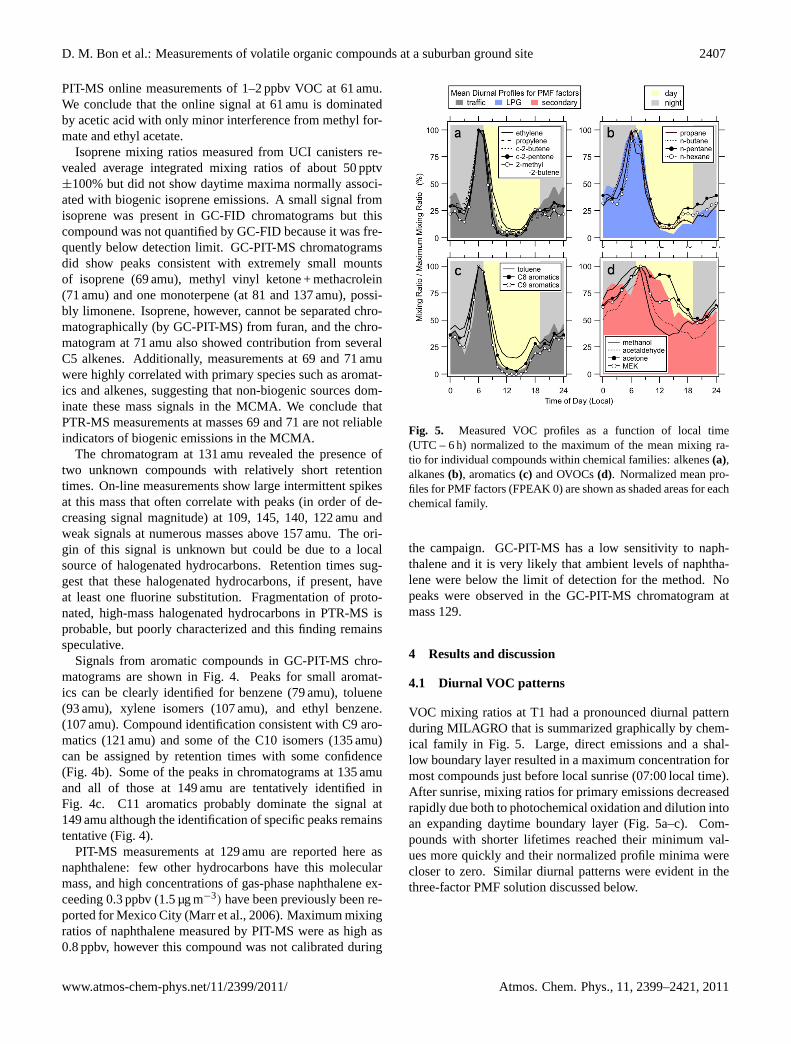
Fig. 5. Measured VOC profiles as a function of local time(UTC – 6 h) normalized to the maximum of the mean mixing ra-tio for individual compounds within chemical families: alkenes(a),alkanes(b), aromatics(c) and OVOCs(d). Normalized mean pro-files for PMF factors (FPEAK 0) are shown as shaded areas for eachchemical family.

the campaign. GC-PIT-MS has a low sensitivity to naph-thalene and it is very likely that ambient levels of naphtha-lene were below the limit of detection for the method. Nopeaks were observed in the GC-PIT-MS chromatogram atmass 129.

4 Results and discussion

4.1 Diurnal VOC patterns

VOC mixing ratios at T1 had a pronounced diurnal patternduring MILAGRO that is summarized graphically by chem-ical family in Fig. 5. Large, direct emissions and a shal-low boundary layer resulted in a maximum concentration formost compounds just before local sunrise (07:00 local time).After sunrise, mixing ratios for primary emissions decreasedrapidly due both to photochemical oxidation and dilution intoan expanding daytime boundary layer (Fig. 5a–c). Com-pounds with shorter lifetimes reached their minimum val-ues more quickly and their normalized profile minima werecloser to zero. Similar diurnal patterns were evident in thethree-factor PMF solution discussed below.



41

1009 Figure 6. Average fraction of total PIT-MS signal attributed to oxygenates, aromatics and other 1010

identified signal during the MILAGRO campaign. Unidentified signal averages about 18% of the 1011

total. 1012

Fig. 6. Average fraction of total PIT-MS signal attributed to oxy-genates, aromatics and other identified signal during the MILAGROcampaign. Unidentified signal averages about 18% of the total.

Photochemical production of oxygenated species leads toa very different diurnal profile. The balance of the produc-tion and the dilution in an expanding boundary layer causesmixing ratios for most OVOCs to decline more slowly aftersunrise than those with exclusively primary sources (Fig. 5d).The atmospheric processing of primary emissions and pro-duction of secondary products is discussed in detail else-where (de Gouw et al., 2009).

The fraction of the PIT-MS signal that could not be at-tributed to specific compounds is shown in Fig. 6 as a func-tion of the time of day. The unidentified signal averaged 18%of the total for the entire campaign, a result which is consis-tent with previous estimates of unidentified signal from fieldmeasurements with PIT-MS (Warneke et al., 2005b). Dur-ing the campaign, the majority of PIT-MS signal can be at-tributed to compounds clearly identified using GC-PIT-MS(Fig. 6).

4.2 Urban emission ratios

4.2.1 Hydrocarbons

The early morning maximum in most VOCs is due to theaccumulation of primary emissions in a shallow boundarylayer in the absence of significant chemical removal. There-fore, these data are very useful for the determination of urbanemission ratios. Most VOCs with primary sources only (hy-

drocarbons) showed a high degree of correlation with inertcombustion tracers such as carbon monoxide (CO) (Fig. 7).Most alkenes and aromatics were also strongly (r2 > 0.70)correlated with carbon monoxide (Table 3). Propane, n-butane and i-butane correlated poorly with CO, as their emis-sions are likely dominated by leakage of liquid propane gas(LPG) rather than combustion (Blake and Rowland, 1995).Figure 7f shows the contrast between morning and after-noon measurements for PIT-MS measurements of the C8-aromatics.

Here we derive emission ratios from the slopes of two-sided (ODR) fits of the VOC data versus CO. Table 3 sum-marizes these emission ratios for all measured hydrocarbons.Emission ratios for important VOCs not measured by GC-FID or PIT-MS (e.g. ethane, C7 and higher alkanes, and ben-zene) were calculated from UCI canister measurements ofthese compounds and CO. In Table 3 we report both the 1-sigma uncertainty in the regression slope and the calibrationuncertainty. We note that the emission ratios presented herefor ethane and propane differ substantially from those cal-culated by Apel et al. (2010), which were derived from l-sided linear regression fits. Because of the poor correlationof ethane and propane with CO, their ratios versus CO have alimited value and a very large uncertainty. We are includingthem here for the sake of completeness.

4.2.2 Oxygenated VOCs

Many OVOCs have both direct emission sources and areformed photochemically. In an urban environment, sourcesof OVOCs from combustion are likely minor compared withthose from industrial, evaporative and particularly photo-chemical sources. As a result, poor correlation with CO is ex-pected and observed for most OVOCs (Fig. 8). Figure 8 alsoillustrates the large difference in mixing ratios for OVOCs inthe morning and afternoon period. Fits made in the plots ofmorning OVOC mixing ratios versus CO tend to parallel thelower edge of the data (closest to the CO axis) suggestinga method for estimating OVOC measurements that might beuseful in future studies.

Emission ratios versus CO were calculated from slopes ofODR fits for measurements made between 04:00 and 07:00local time in order to minimize the effects of photochemicalproduction. The results are shown by solid, black lines inFig. 8 and summarized in Table 4.

4.2.3 Comparison of emission ratios with those fromUS cities

Emission ratios for hydrocarbons versus CO from measure-ments made in the United States (Baker et al., 2008; Warnekeet al., 2007) are added to Fig. 7 and to Table 3 for com-parison purposes. For most alkenes and aromatics, MexicoCity emission ratios to CO are approximately a factor of twolarger than corresponding values from the United States. The



Table 3. Urban emission ratios for non-methane hydrocarbons quantified during MILAGRO versus carbon monoxide are compared to PMF-derived emission ratios and values for US cities from the literature. Correlation coefficients (r2) and the number of points fit(N) are shownfor measurement derived emission ratios. Reported errors for measurement-derived emission ratios are 1σ uncertainties in the slope of theODR fit. Uncertainties reported for the PMF-derived emission ratios were calculated using the method described in the text.

Compound MILAGRO calibration r2 N New England 28 US cities MILAGRO PMFEmission Ratio uncertainty Warneke et al. Baker et al. EmissionBest Estimat (2007) (2008) Ratiod,e

2006 2004 1999–2005(pptv [ppbv CO]−1) (%) (pptv [ppbv CO ]−1)

Alkanes

ethanea 21.5± 10.8 10 % 0.50 199 11.62 2.4propaneb 61.7± 15.6 10 % 0.53 1242 7.73 3.8 43.5± 4.1n-butaneb 21.7± 5.0 10 % 0.57 1242 1.69 1.4 17.3± 1.5i-butaneb 7.2± 1.6 10 % 0.57 1242 1.01 0.9 6.0± 0.5n-pentaneb 2.5± 0.2 10 % 0.81 1241 1.55 1.2 2.6± 0.3i-pentaneb 3.3± 0.4 10 % 0.77 1242 3.99 2.9 3.4± 0.4n-hexaneb 1.49± 0.16 10 % 0.70 1240 1.07 0.6 1.0± 0.1cyclopentanea 0.153± 0.008 10 % 0.88 166cyclohexanea 0.164± 0.008 10 % 0.77 181 0.29methyl cyclopentanea 0.47± 0.02 10 % 0.87 194 0.572,2-dimethyl butanea 0.36± 0.02 10 % 0.89 159 0.122,3-dimethyl butanea 1.67± 0.13 10 % 0.72 160 0.272-methyl pentanea 1.33± 0.07 10 % 0.89 165 1.113-methyl pentanea 0.90± 0.05 10 % 0.91 166 1.28n-heptanea 0.36± 0.06 10 % 0.69 199 0.40 0.22,4-dimethyl pentanea 0.126± 0.006 10 % 0.87 187 0.17n-octanea 0.122± 0.006 10 % 0.33 152 0.20 0.1n-nonanea 0.065± 0.003 10 % 0.32 158n-decanea 0.042± 0.002 10 % 0.26 182 1.E-04

Alkenes

ethyleneb 7.0± 0.4 10 % 0.90 1242 4.56 4.1 7.1± 0.9propyleneb 3.0± 0.2 10 % 0.86 1242 1.36 1.0 2.8± 0.41-buteneb 0.35± 0.02 10 % 0.87 1236 0.14 0.2 0.32± 0.042-methyl propeneb 0.85± 0.04 10 % 0.91 1236 0.76± 0.11cis-2-buteneb 0.18± 0.02 10 % 0.82 1236 0.06 0.16± 0.02trans-2-buteneb 0.20± 0.02 10 % 0.82 1235 0.05 0.16± 0.021-penteneb 0.152± 0.011 10 % 0.88 1211 0.15± 0.02cis-2-penteneb 0.100± 0.009 10 % 0.86 1206 0.05 0.09± 0.02trans-2-penteneb 0.190± 0.017 10 % 0.85 1209 0.17± 0.032-methy 2-buteneb 0.179± 0.019 10 % 0.83 1202 0.15± 0.022-methyl 1-buteneb 0.140± 0.011 10 % 0.87 1213 0.14± 0.023-methy 1-buteneb 0.044± 0.006 10 % 0.80 11951,3-butadienea 0.278± 0.014 10 % 0.84 147

Alkynes

acetyleneb 6.5± 0.3 10 % 0.90 1242 3.60 3.4 5.0± 0.7

Aromatics

benzenea 1.21± 0.06 10 % 0.94 183 0.62 0.7toluenec 4.2± 0.4 20 % 0.69 2563 2.62 2.7 4.0± 0.46C8 aromaticsc 4.3± 0.6 50 % 0.71 2563 1.93 3.8± 0.569 aromaticsc 2.8± 0.6 50 % 0.79 2563 1.07 2.3± 0.46C10 aromaticsc 0.76± 0.15 50 % 0.71 2563 0.60± 0.14611 aromaticsc 0.16± 0.03 50 % 0.41 2563 0.12± 0.01naphthalenec 0.12± 0.01 50 % 0.24 2592 0.11± 0.01

a UCI-canisters, data from entire campaign.b NOAA GC-FID, data from entire campaign.c NOAA PIT-MS, data from 04:00–07:00 a.m., local time.d Calculated using6 (traffic + LPG) factors;r2

= 0.86 with CO for PMF traffic factor andr2= 0.56 for LPG factor.

e N = 851 for emission ratios derived from PMF analysis.



Table 4. Urban emission ratio estimates versus CO for OVOCs and acetonitrile calculated by linear regression and from MILAGRO mea-surements and from the results of PMF analysis. For comparison, literature values from PTR-MS measurements made in New England andfrom a US tunnel study are also shown. Methods used to calculate these values are discussed in detail in the text. Also shown are correlationcoefficients (r2) and the number of points fit(N). Reported errors for measurement-derived emission ratios are 1σ uncertainties in the slopeof the ODR fit. Uncertainties reported for the PMF-derived emission ratios were calculated using the method described in the text.

MILAGRO calibration r2 N New England Caldecot Tunnel MILAGRO PMFEmission Ratio uncertainty Warneke et al. Ban-Weiss et al. (2008) EmissionBest estimate (2007) Ratiob,d

2006a 2004 1999 2001 2006 Diesel(pptv [ppbv CO]−1) (%) (pptv [ppbv CO]−1)

Oxygenates

methanol 2.1± 0.5 20 % 0.11 2563 4.0 6.1± 2.1acetaldehyde 1.0± 0.3 20% 0.23 2563 0.7 1.0 0.5 0.7 12.0 2.0± 0.9formic acidc 0.22± 0.11 50 % 0.12 2592 0.4± 0.3acetone 0.51± 0.13 20% 0.06 2563 2.9 0.7 0.4 1.0± 1.0acetic acid 0.5± 0.2 50 % 0.09 2563 0.5± 0.5MEK 0.29± 0.07 20% 0.13 2563 0.8 0.1 0.1 0.2 1.4 0.5± 0.3

Other

acetonitrile 0.27± 0.07 20% 0.24 2563 0.4± 0.1

a Ratios calculated from PIT-MS data collected between 04:–07:00 a.m. LT.b Calculated using6 (traffic + LPG) factors;r2

= 0.86 with CO for PMF traffic factor andr2= 0.56 for LPG factor.

c For purposes of PMF, formic acid was included as one of the 65 unquantified PIT-MS measurements.d N = 851 for PMF-derived emission ratios.

42

1013 Figure 7. Selected plots used to calculate urban emission ratios (ERs) with respect to carbon 1014

monoxide (CO) for VOC measurements made by GC-FID (a-d), canister samples (e) and PIT-MS (f). 1015

Urban ERs calculated from measurements using ODR fits (black) and Positive Matrix Factorization 1016

results (purple) during MILAGRO. MCMA ERs are compared to literature values (red, green) 1017

obtained for cities in the United States. PIT-MS measurements are shown on a 1-minute time base (f) 1018

to highlight mixing ratio differences prior to local sunrise (grey) versus those observed during the 1019

mid-afternoon (yellow). PMF lines represent ERs obtained by summing the traffic and LPG factors. 1020

Fig. 7. Selected plots used to calculate urban emission ratios (ERs) with respect to carbon monoxide (CO) for VOC measurements made byGC-FID (a–d), canister samples(e) and PIT-MS(f). Urban ERs calculated from measurements using ODR fits (black) and Positive MatrixFactorization results (purple) during MILAGRO. MCMA ERs are compared to literature values (red, green) obtained for cities in the UnitedStates. PIT-MS measurements are shown on a 1-minute time base(f) to highlight mixing ratio differences prior to local sunrise (grey) versusthose observed during the mid-afternoon (yellow). PMF lines represent ERs obtained by summing the traffic and LPG factors.



43

1021 Figure 8. Plots used to calculate emission ratios with respect to carbon monoxide (CO) for 5 OVOCs 1022

quantified by PIT-MS. Emission ratios calculated from measurements using 2-sided regression fits 1023

(black) and Positive Matrix Factorization results (purple) during MILAGRO are compared to 1024

literature values obtained during field studies in New England (red) and to a California tunnel study 1025

(blue). 1-Minute PIT-MS data show afternoon enhancements in OVOCs typically observed during 1026

the campaign. For comparison purposes, lines showing PMF and literature ERs are shown with 1027

intercepts obtained from ODR fits of MILAGRO measurements. PMF lines represent ERs obtained 1028

by summing the traffic and LPG factors. 1029

Fig. 8. Plots used to calculate emission ratios with respect to carbon monoxide (CO) for 5 OVOCs quantified by PIT-MS. Emission ratioscalculated from measurements using 2-sided regression fits (black) and Positive Matrix Factorization results (purple) during MILAGRO arecompared to literature values obtained during field studies in New England (red) and to a California tunnel study (blue). 1-Minute PIT-MS data show afternoon enhancements in OVOCs typically observed during the campaign. For comparison purposes, lines showing PMFand literature ERs are shown with intercepts obtained from ODR fits of MILAGRO measurements. PMF lines represent ERs obtained bysumming the traffic and LPG factors.

difference is probably due to differences in automobile emis-sion systems and fleet ages between the two countries. CO toCO2 ratios of about 45 ppbv ppmv−1 were observed duringthe MILAGRO campaign (Vay et al., 2009); a value simi-lar to the ratio observed in plumes originating in China andtwice as large as the 10–20 ppbv ppmv−1 observed in indus-trialized nations like Japan and the United States (de Gouwet al., 2004; Takegawa et al., 2004). It is worth noting, there-fore, that VOC emission ratios per kg fuel burned are prob-ably closer to a factor of 6± 2 larger in Mexico City thanthose for US cities.

Emission ratios for OVOCs from 2004 measurements inNew England and those from a 1999 California tunnel studyare shown in Fig. 8 and Table 4 (Warneke et al., 2007; Ban-Weiss et al., 2008). OVOC emission ratios for Mexico Citymore closely resemble values obtained in the tunnel studythan those calculated from measurements in the Northeast-ern US Differences between OVOC emission ratios from theMCMA and the Northeastern US could be due to samplingmethodology, i.e. the Northeastern US data were largely col-lected outside city boundaries and although an attempt wasmade to account for the effects of secondary production us-ing a photochemical lifetime method, the resulting emissionratios may still overestimate the direct emissions. Biogenicemissions may also account for some of the differences ob-

served between Mexico City and New England, particularlyfor methanol, which has significant biogenic sources (Jacob,2005; Millet et al., 2008).

4.3 PMF Results

4.3.1 The PMF solution

PMF solutions with 1 to 7 factors were examined using themethod described in Sect. 2.3. A three-factor solution waschosen based on the plausibility of the results, with factorsidentified as traffic, LPG leakage, and secondary + long-livedspecies, described individually in more detail below. This so-lution hasQ/Qexp= 4.07 at FPEAK 0, which suggests thatthe errors may be somewhat underestimated or that there issubstantial variability in the dataset that cannot be modeledwell with a few fixed chemical profiles.Q/Qexp increasesby less than 10% over the range in FPEAK from−5 to +5.Over the narrower FPEAK range from−3 to +3,Q/Qexp in-creases by 2% compared to the FPEAK 0 solution. Measure-ments from each instrument contributed 44± 0.1 % (GC-FID) and 56± 0.1 % (PIT-MS) to the parameter(Q) overthe range from FPEAK−3 to +3. About 20% of the value ofQ could be attributed to unidentified PIT-MS signal.



44

1030 Figure 9. PMF profiles are shown for compounds measured by the NOAA GC-FID (left column) and 1031

NOAA PIT-MS (right column) for the three factors, here labeled traffic, LPG, and secondary + long-1032

lived species. Error bars represent the variation in PMF factors from the FPEAK=0 solution (solid 1033

bars) over the FPEAK range from -3.0 to +3.0 as described in the text. 1034

Fig. 9. PMF profiles are shown for compounds measured by the NOAA GC-FID (left column) and NOAA PIT-MS (right column) forthe three factors, here labeled traffic, LPG, and secondary + long-lived species. Error bars represent the variation in PMF factors from theFPEAK 0 solution (solid bars) over the FPEAK range from−3.0 to +3.0 as described in the text.

Source profiles for the 3-factor solution are shown inFig. 9. The first factor, referred to as “traffic” from now on, iscomprised of hydrocarbons including highly reactive speciesand was easily recognized as the VOCs observed during theearly-morning maximum. The profile of the second factor,named “LPG,” contains propane and other small alkanes andis likely associated with LPG leakage. The third factor isnamed “secondary + long-lived species” and is comprised ofinert hydrocarbons and oxygenated species, and resemblesthe VOCs observed in more processed air masses observedduring the day. In PMF solutions with 4 or more factors, ad-ditional factors resembled combinations of the three factorsand did not provide additional insight into the data. Despitethe presence of gas-phase chemical tracers for biogenic emis-sions (e.g. isoprene), biomass burning (e.g. acetonitrile), andknown industrial emissions within the MCMA (Fortner et al.,2009), no factors were identified in the PMF analysis thatwere direct representations of these emission sources duringthis study. A more detailed individual description of the threefactors can be found below.

Figure 10 shows the variability in apportionment of afew important VOCs over the range of FPEAKS−3 to +3.Changes in the apportionment of individual compounds with

FPEAK have no clear physical interpretation. For example,the apportionment of n-butane to the three factors changessharply at FPEAKS above +1.5, where n-butane is attributedalmost completely to the LPG factor, consistent with its ex-pected source from LPG leakage as discussed above; how-ever, the apportionments at FPEAKs less than−0.5, withsignificant contributions of n-butane to the traffic and sec-ondary + long-lived species is also plausible and consistentwith the lifetime of n-butane and its emissions in vehicle ex-haust. Acetone shows an opposite behavior with respect toFPEAK, where solutions with FPEAK greater than +2 appor-tion acetone exclusively to the secondary + long-lived speciesfactor, which does not reflect its known sources from traf-fic. Thus, no single FPEAK value produces a solution thatis uniquely best. Therefore, the solutions presented hereinare for FPEAK 0 with the range of solutions with FPEAKof ±3 are reported as an estimate of the uncertainty in thefactor profiles and time series. We speculate that some ofthe variability in apportionment with FPEAK in this anal-ysis is explained by the lack of strong contrast in the timetrends of different species during the night when all directemissions accumulate in the shallow boundary layer andchemical processing of the air mass is at its daily minimum.



45

1035 Figure 10. Variability in apportionment to factors as a function of the PMF rotational parameter 1036

FPEAK for acetone, n-butane and three hydrocarbons dominated by traffic emissions (acetylene, 1037

toluene and propylene). The change in the PMF quality of fit parameter is less than 2% for the 1038

FPEAK values shown. 1039

1040

Fig. 10. Variability in apportionment to factors as a function of the PMF rotational parameter FPEAK for acetone, n-butane and threehydrocarbons dominated by traffic emissions (acetylene, toluene and propylene). The change in the PMF quality of fit parameter is less than2% for the FPEAK values shown.

Other methods used to estimate uncertainties in the analyses,e.g. bootstrapping and seed variation (Ulbrich et al., 2009),were investigated but gave smaller variation in factor pro-files. The three-factor solution was investigated as a functionof the weighting errors assumed for the GC-FID and PIT-MSdata. None of the observed variation changed the conclusionsdrawn here in any significant way. A more comprehensiveanalysis of the effects on PMF analysis of relative weightingof the data from different instruments can be found elsewhere(Slowik et al., 2010).

The averaged diurnal variation in the factor time series isshown in Fig. 11. Briefly, the traffic factor consists of aro-matics, alkenes, alkanes and acetylene, and is at its maximumin the early morning. The LPG factor consists predominantlyof propane, n-butane and i-butane and also has a maximum inthe morning. The secondary + long-lived species factor is atits maximum about 2 h later than the traffic factor and falls offmuch more slowly after sunrise. The averaged diurnal varia-tions in factor time series were overlaid with the VOC data inFig. 5. The traffic factor closely follows the diurnal variationsin the more reactive alkenes and aromatics. The LPG factoris very similar to the measured diurnal variations in propaneand other alkanes. The secondary + long-lived species factordoes not directly match the diurnal variation of any singleoxygenated species, but approximates the ensemble averagediurnal variation of the oxygenated species shown.

The PMF reconstructions of the time series of selectedVOCs are shown for acetylene, n-butane and acetone atFPEAK 0 in Fig. 12. The variability in acetylene mea-surement is well described by the PMF time-series recon-struction (r2

= 0.89) and the majority of this compound isattributed to traffic sources. The variability in n-butane isalso reasonably well described by the PMF time-series re-construction (r2

= 0.76). In this case, most of the signal isattributed to LPG leakage. The measurement of acetone andits PMF time-series reconstruction (Fig. 12c) correlate well(r2

= 0.93) and most of the signal is attributed to the sec-ondary + long-lived species factor with a smaller contributionfrom the traffic factor. Large residuals between measured andreconstructed concentrations were frequently correlated withsimultaneous spikes in several VOCs without correspondingchanges in CO mixing ratios. Examples of such spikes canbe seen in Fig. 12 for acetylene and n-butane and they sug-gest the presence of local emissions, the variability of whichis difficult to capture with PMF if the plume composition issufficiently different from the dominant sources of variation.

Time series reconstructions for other species were com-pared to the measurements (results not shown here). Lin-ear correlation coefficients were high for C7-C10 aromat-ics, alkenes and acetylene (r2 > 0.85) and slightly lowerfor methanol, acetone, acetaldehyde and MEK (0.82 <

r2 < 0.90). PMF reconstructions for alkanes and the



46

1040 Figure 11. Mean diurnally averaged profiles for the 3-factor PMF solution obtained from MILAGRO 1041

VOC measurements. Solid lines represent the mean diurnal profile for each factor at FPEAK 0 while 1042

the shaded regions bordered with dashes show the variation from the FPEAK = 0 solution over the 1043

FPEAK range from -3.0 to +3.0. 1044

Fig. 11. Mean diurnally averaged profiles for the 3-factor PMF so-lution obtained from MILAGRO VOC measurements. Solid linesrepresent the mean diurnal profile for each factor at FPEAK 0 whilethe shaded regions bordered with dashes show the variation fromthe FPEAK 0 solution over the FPEAK range from−3.0 to +3.0.

C11-aromatics correlated reasonably well with measure-ments (0.60< r2 < 0.88). Much lower correlations werefound for acetonitrile (r2

= 0.42), acetic acid (r2= 0.48),

and naphthalene (r2= 0.55). Correlations for these species

did not improve significantly even when PMF solutions withgreater than three factors were considered (p > 3). Poor fitsfor these compounds in the PMF analysis suggest that theyhave important sources that are not correlated with the threefactors identified here. For acetonitrile, the explanation maybe the presence of biomass burning sources (de Gouw et al.,2009) that were not identified as a separate factor in the PMFanalysis.

4.3.2 PMF traffic factor

The profile of the traffic factor is shown in Fig. 9 (top pan-els). The profile is dominated by alkenes and aromatics. C5and higher alkanes are also present. The only OVOC withsignificant partitioning to the traffic factor was methanol.Methanol mixing ratios were substantial during MILAGROand have likely contributions from tailpipe and other vehicu-lar sources previously observed by vehicle emission studiesin the MCMA (Rogers et al., 2006) or by industrial sources.

The PIT-MS product-ion signal at 57 amu was predomi-nantly apportioned to the traffic factor, which is consistentwith the major contribution of the gasoline additive MTBE tom57 (∼80%), as determined by GC-PIT-MS (Fig. 3). Otherproduct ion signals with significant presence in the trafficfactor are at 69, 71, 83 and 85 amu. The signals at 69 and71 amu are typically used to quantify isoprene and its pho-toproducts MVK and methacrolein in PTR-MS. This analy-

sis suggests that the importance of other species with traffic-related sources (such as the presence of C5-alkenes at 71 amushown in Fig. 3) at these masses in Mexico City can be shownwith PMF analysis. The absence of a PMF factor represent-ing biogenic emissions for compounds measured atm/z69and 71 by PIT-MS is consistent with the observations aboutthe signal at these masses (e.g. low mixing rations, correla-tion with CO and GC-PIT-MS results) discussed elsewherein this text.

4.3.3 PMF LPG factor

The LPG factor profile is dominated by the three light alka-nes (propane, n-butane and i-butane) associated with lique-fied petroleum gas use in the MCMA (Fig. 9, middle panel)(Blake and Rowland, 1995; Vega et al., 2000; Velasco et al.,2007). The reconstruction of n-butane in the 3-factor PMFsolution is compared with its measurement in Fig. 12 (mid-dle panel). The three major LPG alkanes also contribute tothe traffic factor, possibly because LPG is used as a vehiclefuel (Diaz et al., 2000), and also to the secondary + long-livedspecies factor, due to their lower reactivity with the hydroxylradical (kOH) as discussed below. However, the contributionof propane to these factors is strongly dependent on FPEAK(Fig. 10) and therefore not well-quantified by this analysis.

Other compounds apportioned to this factor include otherlight alkanes, some traffic-related VOCs and methanol, butthe amount of signal associated with the LPG factor for theseother VOCs decreases as a function of FPEAK. The diurnallyaveraged profile for the LPG factor has a similar shape tothat of the traffic factor, but has a larger magnitude and widermorning maximum (Fig. 11) probably due to the longer pho-tochemical lifetime of major LPG species.

4.3.4 PMF secondary + long-lived species factor

The profile for the secondary + long-lived species factor con-sists of mostly oxygenated compounds: methanol, acetone,acetaldehyde, acetic acid, methyl ethyl ketone (MEK), andformic acid. For all quantified OVOCs except acetic acid, atleast 66% of the measured concentration was explained bythis factor. Good agreement was found between PMF recon-structions and measurements of methanol, acetone, acetalde-hyde, and butanone (MEK) (slopes>0.90 andr2 > 0.80).Although acetic acid, formic acid and acetonitrile receivedmajority apportionment to the secondary + long-lived speciesfactor, measurements of these compounds correlated poorly(r2 < 0.50) with PMF reconstructions. Variation in the mix-ing ratios of these 3 compounds were not well explained bythe PMF analysis. These results could suggest additionalsources for these compounds. However, instrument precisionalso limits the degree of correlation for these species.

The relative contribution to the secondary + long-livedspecies factor increased with FPEAK for all quantifiedOVOCs and acetonitrile. Because OVOCs have known



47

1045 Figure 12. Selected comparisons between measurements and PMF reconstructions for one period 1046

during the MILAGRO campaign. The left column shows time series for representative compounds 1047

with dominant apportionment to the traffic factor (acetylene), the LPG factor (n-butane) and the 1048

secondary + long-lived factor (acetone). Measurements are shown as solid black traces for 1049

comparison. On the right are scatter plots of PMF reconstructions versus measurements showing 1050

single-sided fits (black) and 1:1 lines (red) for the same compounds. 1051

1052

Fig. 12. Selected comparisons between measurements and PMF reconstructions for one period during the MILAGRO campaign. The leftcolumn shows time series for representative compounds with dominant apportionment to the traffic factor (acetylene), the LPG factor (n-butane) and the secondary + long-lived factor (acetone). Measurements are shown as solid black traces for comparison. On the right arescatter plots of PMF reconstructions (FPEAK 0) versus measurements showing single-sided fits (black) and 1:1 lines (red) for the samecompounds.

vehicular emission sources (Rogers et al., 2006), the nearabsence of OVOCs from the traffic factor at FPEAKS>2.0provides a physical constraint on the results of PMF analysis.An example such a change in the apportionment of an OVOCis shown for acetone in Fig. 10.

A comparison of measurements and PMF reconstructionsfor acetone are shown in Fig. 12 (bottom left panel). Thediurnal average for the PMF secondary + long-lived factorlooks similar to the measured diurnal profiles of OVOCs(Fig. 5d), although diurnally averaged measurements ofOVOCs show considerably more variation as a group thando hydrocarbons.

PIT-MS product-ion signals at masses 75, 87, 89, and101 amu were mainly attributed to the secondary + long-livedfactor. This suggests the presence of OVOCs at these masses.Specifically, it is possible that propanoic and butanoic acidscontributed to the signal at masses 75 and 89.

4.3.5 Estimation of VOC emission ratios using PMFresults

Linear regression (ODR) of individual PMF factors plottedversus CO showed that the traffic factor correlated well withCO (r2

= 0.86) in the predawn period but showed no correla-tion after noon.The LPG and secondary + long-lived speciesfactors showed poor correlation with CO in the morning but



stronger correlations in the afternoon (r2= 0.81, 0.77 respec-

tively). To estimate urban emission ratios for VOCs andOVOCs in the MCMA from the PMF results, the sum ofthe contributions of the traffic and LPG factors were plottedagainst CO (r2 < 0.42) measurements for the 30 compoundsquantified and reported during the campaign plus formic acid(m/z47). The slopes of the resulting plots are presented inTables 3 and 4 for VOCs and OVOCs respectively.

The relative uncertainties (1σ ) in the slopes of the lin-ear regression used to calculate PMF-derived emission ratioswere small (1–3%) for all compounds. Uncertainty in PMF-derived emission ratios was also assessed using changes inapportionment as a function of the PMF FPEAK parame-ter. The maximum relative difference in apportionment fromFPEAK 0 over the range from FPEAK−3 to 3 for the sumof the traffic and LPG source profiles was larger (4%–100%)than the regression uncertainty for all compounds. The sumof the relative uncertainties for each compound were used tocalculate the absolute uncertainties in PMF-derived emissionratios shown in Tables 3 and 4.

Emission ratios calculated from PMF results are com-pared to values calculated directly from VOC measurementsin Fig. 13. Individual points represent VOC species andare colored according to the PMF factor that explained themajority of the variation of that species. Emission ra-tios estimated for compounds mainly associated with trafficand LPG emissions were systematically lower by 20% thanthose derived directly from measurements, while the valuesof PMF-derived emission ratios for secondary + long-livedcompounds were larger by an average of 80%. As describedin Sect. 4.2.2 above, emission ratios for OVOCs were calcu-lated only from the measured data from 04:00 to 07:00 localtime, when the direct emissions should dominate the vari-ability of these species. Emission ratios for OVOCs esti-mated from the traffic + LPG factors from the PMF analy-sis attempt to include only the directly emitted fraction ofthe OVOCs. Thus, both methods used here for calculatingOVOC emission ratios attempt to correct measurements forsecondary production. Uncertainty in the emission ratios cal-culated from PMF results is dominated by the uncertaintiesin the PMF results, particularly strongly for OVOCs.

4.3.6 Limitations of the PMF analysis as applied toVOC measurements

Some limitations of the application of PMF to VOC mixingratios became apparent over the course of this work. First,the bilinear unmixing model makes the assumption that thespecies identified together in one factor occur in constant rel-ative proportions over the entire measurement period. How-ever, individual VOCs and OVOCs have photochemical life-times (kOH) that span several orders of magnitude, and soVOCs emitted from a single source are removed in the at-mosphere at very different rates and thus the ratios of theirconcentrations will change continuously. This helps explain

48

1053 Figure 13. Comparison of PMF emission ratio estimates obtained by linear regression for all 1054

measured compounds. Each point represents one compound while colors represent the dominant 1055

PMF apportionment for the respective measurement. 1056

1057

Fig. 13. Comparison of PMF emission ratio estimates obtained bylinear regression for all measured compounds. Each point repre-sents one compound while colors represent the dominant PMF ap-portionment for the respective measurement.

the way individual VOCs are apportioned between the fac-tors. For example, the traffic factor closely matches the diur-nal variability of the shortest-lived compounds that have lowmixing ratios, while primary hydrocarbons with long life-times are partially explained by the secondary + long-livedspecies factor in proportion to their photochemical lifetimes(Fig. 14), because they are still present in highly processedair. As another example, strict interpretation of the PMF fac-tors (Fig. 9) as sources would suggest that a small portion oftoluene and methanol can be attributed to LPG leakage andthat benzene and propane are partially attributed to secondaryformation, even when this contradicts our knowledge of thesources of these compounds. Thus, the PMF factors identi-fied for this dataset reflect the convolution of VOC sourcesand VOC lifetimes, and interpretation of the factor profilesstrictly in terms of different sources is inappropriate.

Second, for this dataset, the fraction of the variation forsome important LPG and OVOC species (e.g., n-butane andacetone) explained by each factor was strongly dependent onthe FPEAK parameter (Fig. 10). Known characteristics ofsources and lifetimes for these VOCs did not help to signif-icantly narrow the range of FPEAKs of plausible or physi-cally reasonable solutions. For some species, therefore, it isdifficult to quantify the fraction emitted by particular sourceswith much certainty.



49

1057 Figure 14. PMF apportionment of measured compounds to the secondary + long-lived factor plotted 1058

versus photochemical lifetime (kOH) (Atkinson and Arey, 2003). Longer lifetimes are associated with 1059 higher secondary + long-lived source apportionment. Colored bars represent the range of lifetimes by 1060 compound class for alkanes (green), aromatics (black) and alkenes (red). Error bars represent 1061 variability in apportionment due to PMF FPEAK parameter from -3 to 3. 1062

Fig. 14. PMF apportionment of measured compounds to the sec-ondary + long-lived factor plotted versus photochemical lifetime(kOH) (Atkinson and Arey, 2003). Longer lifetimes are associatedwith higher secondary + long-lived source apportionment. Coloredbars represent the range of lifetimes by compound class for alkanes(green), aromatics (black) and alkenes (red). Error bars representvariability in apportionment due to PMF FPEAK parameter from−3 to 3.

5 Conclusions

Two ground-based NOAA instruments were deployed duringthe MILAGRO campaign that provided quantitative analysisof 30 VOCs. Comparison of measurements from these twoinstruments with canister samples and two mobile PTR-MSinstruments was performed and the measurements agreedwithin uncertainty estimates for most compounds.

PIT-MS provided on-line quantification of 12 VOCs andwas used to monitor an additional 150+ product ion masses.The full mass scan of the PIT-MS instrument proved use-ful in identifying signal that might have been missed by aquadrupole PTR-MS and the use of the GC pre-separationmethod provided valuable identification and validation ofPIT-MS measurements during the study. Many species quan-tified by the PIT-MS showed little evidence of interferencefrom other compounds. About 85% of the total PIT-MSsignal arose from identified compounds. Signals at 69 and71 amu, commonly associated with biogenic emissions atother locations, appear to be dominated by traffic emissionsin the MCMA. Product ion masses 69, 71, 75, 85, and 87 amuaccounted for a large fraction of the unidentified signal fromPIT-MS.

Values for VOC and OVOC emission ratios with respect toCO were reported from Mexico City are presented and com-pared with previously reported values from US cities. UrbanVOC emissions in the MCMA are dominated by traffic emis-sions and LPG usage. Emission ratios to CO for most hydro-carbons are generally about a factor of two larger than in theUnited States, while emission ratios to CO2 are likely a factorof (6± 2) larger than US values. Urban OVOC emission ra-tios in Mexico City, calculated by two different methods ap-pear consistent with vehicular sources of these compounds,although measurement uncertainties are large.

Positive Matrix Factorization analysis performed on thecombined data from the two NOAA instruments allowed theidentification of 3 dominant factors: traffic, LPG usage andsecondary production and long-lived species. These factorsdescribed much of the variability in VOC mixing ratios, es-pecially for compounds with vehicular and liquid propanegas sources. OVOCs and compounds with long photochemi-cal lifetimes were identified as a single factor in the analysis.PMF solutions with more than 3 factors resulted in splittingof major factors rather than the identification of minor emis-sion sources. The PMF analysis did not identify distinct fac-tors consistent with industrial, biomass burning or biogenicVOC emissions. Factor profiles (grouping of VOC species)are influenced by both sources and photochemical lifetimesof individual VOCs.

PMF results were also used to estimate emission ratios forVOCs and OVOCs. Estimates agreed within uncertaintieswith the corresponding emission ratios derived directly frommeasurements for most hydrocarbons typically associatedwith vehicle usage. PMF-derived emission ratios were about20% lower and 80% higher for light alkanes and OVOCs re-spectively. We conclude that PMF describes major VOCswell, but strongly caution against the over-interpretation ofPMF factors as strictly corresponding to sources of VOCsbecause the factors may reflect combinations of sources andphotochemical lifetimes, and because solutions may not beunique with respect to rotation.

Acknowledgements.This publication was also developed undera STAR Research Assistance Agreement No. FP-9163901-0awarded by the US Environmental Protection Agency. It has notbeen formally reviewed by the EPA. The views expressed in thispublication or other work are solely those of its authors. The EPAdoes not endorse any products or commercial services mentionedin this publication. This work was also financially supported bythe National Science Foundation under grants ATM-0516610 andATM-0513035.

Edited by: L. Molina



References

Apel, E. C., Calvert, J. G., and Fehsenfeld, F. C.: The NonmethaneHydrocarbon Intercomparison Experiment (NOMHICE) – Task-1 and Task-2, J. Geophys. Res.-Atmos., 99, 16651–16664, 1994.

Apel, E. C., Emmons, L. K., Karl, T., Flocke, F., Hills, A. J.,Madronich, S., Lee-Taylor, J., Fried, A., Weibring, P., Walega, J.,Richter, D., Tie, X., Mauldin, L., Campos, T., Weinheimer, A.,Knapp, D., Sive, B., Kleinman, L., Springston, S., Zaveri, R., Or-tega, J., Voss, P., Blake, D., Baker, A., Warneke, C., Welsh-Bon,D., de Gouw, J., Zheng, J., Zhang, R., Rudolph, J., Junkermann,W., and Riemer, D. D.: Chemical evolution of volatile organiccompounds in the outflow of the Mexico City Metropolitan area,Atmos. Chem. Phys., 10, 2353–2375,doi:10.5194/acp-10-2353-2010, 2010.

Atkinson, R. and Arey, J.: Atmospheric degradation of volatile or-ganic compounds, Chem. Rev., 103, 4605–4638, 2003.

Baker, A. K., Beyersdorf, A. J., Doezema, L., Katzenstein, A.,Meinardi, S., Simpson, I., Blake, D. R., and Rowland, F. S.:Measurements of nonmethane hydrocarbons in 28 United Statescities, Atmos. Environ., 42, 170–182, 2008.

Ban-Weiss, G. A., McLaughlin, J. P., Harley, R. A., Kean, A. J.,Grosjean, E., and Grosjean, D.: Carbonyl and Nitrogen DioxideEmissions From Gasoline-and Diesel-Powered Motor Vehicles,Environ. Sci. Technol., 42, 3944–3950, 2008.

Blake, D. R. and Rowland, F. S.: Urban Leakage of LiquefiedPetroleum Gas and Its Impact on Mexico-City Air-Quality, Sci-ence, 269, 953–956, 1995.

Brown, S. G., Frankel, A., and Hafner, H. R.: Source apportionmentof VOCs in the Los Angeles area using positive matrix factoriza-tion, Atmos. Chem. Phys. Discuss., in preparation, 2010.

Brunekreef, B. and Forsberg, B.: Epidemiological evidence of ef-fects of coarse airborne particles on health, Eur. Resp. J., 26,309–318, 2005.

Buzcu, B. and Fraser, M. P.: Source identification and apportion-ment of volatile organic compounds in Houston, TX, Atmos. En-viron., 40, 2385–2400, 2006.

Colman, J. J., Swanson, A. L., Meinardi, S., Sive, B. C., Blake, D.R., and Rowland, F. S.: Description of the analysis of a widerange of volatile organic compounds in whole air samples col-lected during PEM-Tropics A and B, Anal. Chem., 73, 3723–3731, 2001.

de Gouw, J. A. and Warneke, C.: Measurements of volatile organiccompounds in the Earth’s atmosphere using proton-transfer-reaction mass spectrometry, Mass Spec. Rev., 26, 223–257,2007.

de Gouw, J. A., Goldan, P. D., Warneke, C., Kuster, W. C., Roberts,J. M., Marchewka, M., Bertman, S. B., Pszenny, A. A. P., andKeene, W. C.: Validation of proton transfer reaction-mass spec-trometry (PTR-MS) measurements of gas-phase organic com-pounds in the atmosphere during the New England Air QualityStudy (NEAQS) in 2002, J. Geophys. Res.-Atmos., 108, 4682,doi:10.1029/2003JD003863, 2003.

de Gouw, J. A., Cooper, O. R., Warneke, C., Hudson, P. K., Fehsen-feld, F. C., Holloway, J. S., Hubler, G., Nicks, D. K., Nowak,J. B., Parrish, D. D., Ryerson, T. B., Atlas, E. L., Donnelly, S.G., Schauffler, S. M., Stroud, V., Johnson, K., Carmichael, G. R.,and Streets, D. G.: Chemical composition of air masses trans-ported from Asia to the US West Coast during ITCT 2K2: Fossilfuel combustion versus biomass-burning signatures, J. Geophys.

Res.-Atmos., 109, D23S20,doi:10.1029/2003JD004202, 2004.de Gouw, J. A., Middlebrook, A. M., Warneke, C., et al.: Budget of

organic carbon in a polluted atmosphere: Results from the NewEngland Air Quality Study in 2002, J. Geophys. Res.-Atmos.,110, D16305,doi:10.1029/2004JD005623, 2005.

de Gouw, J. A., Welsh-Bon, D., Warneke, C., Kuster, W. C., Alexan-der, L., Baker, A. K., Beyersdorf, A. J., Blake, D. R., Cana-garatna, M., Celada, A. T., Huey, L. G., Junkermann, W., Onasch,T. B., Salcido, A., Sjostedt, S. J., Sullivan, A. P., Tanner, D.J., Vargas, O., Weber, R. J., Worsnop, D. R., Yu, X. Y., andZaveri, R.: Emission and chemistry of organic carbon in thegas and aerosol phase at a sub-urban site near Mexico City inMarch 2006 during the MILAGRO study, Atmos. Chem. Phys.,9, 3425–3442,doi:10.5194/acp-9-3425-2009, 2009.

Diaz, L., Schifter, I., Lopez-Salinas, E., Gamas, E., Rodriguez, R.,and Avalos, S.: Optimizing automotive LPG blend for Mexicocity, Fuel, 79, 79–88, 2000.

Edgerton, S. A., Bian, X., Doran, J. C., et al.: Particulate air pol-lution in Mexico City: A collaborative research project, J. AirWaste Manage., 49, 1221–1229, 1999.

Engel-Cox, J. A. and Weber, S. A.: Compilation and assessment ofrecent positive matrix factorization and UNMIX receptor modelstudies on fine particulate matter source apportionment for theeastern United States, J. Air Waste Manage., 57, 1307–1316,2007.

Fast, J. D., de Foy, B., Acevedo Rosas, F., Caetano, E., Carmichael,G., Emmons, L., McKenna, D., Mena, M., Skamarock, W.,Tie, X., Coulter, R. L., Barnard, J. C., Wiedinmyer, C., andMadronich, S.: A meteorological overview of the MILA-GRO field campaigns, Atmos. Chem. Phys., 7, 2233–2257,doi:10.5194/acp-7-2233-2007, 2007.

Fast, J., Aiken, A. C., Allan, J., Alexander, L., Campos, T., Cana-garatna, M. R., Chapman, E., DeCarlo, P. F., de Foy, B., Gaffney,J., de Gouw, J., Doran, J. C., Emmons, L., Hodzic, A., Hern-don, S. C., Huey, G., Jayne, J. T., Jimenez, J. L., Kleinman,L., Kuster, W., Marley, N., Russell, L., Ochoa, C., Onasch, T.B., Pekour, M., Song, C., Ulbrich, I. M., Warneke, C., Welsh-Bon, D., Wiedinmyer, C., Worsnop, D. R., Yu, X.-Y., and Zaveri,R.: Evaluating simulated primary anthropogenic and biomassburning organic aerosols during MILAGRO: implications for as-sessing treatments of secondary organic aerosols, Atmos. Chem.Phys., 9, 6191–6215,doi:10.5194/acp-9-6191-2009, 2009.

Finlayson-Pitts, B. J.: Tropospheric Air Pollution: Ozone, AirborneToxics, Polycyclic Aromatic Hydrocarbons, and Particles, Sci-ence, 276, 1045–1051, 1997.

Fortner, E. C. and Knighton, W. B.: Quantitatively resolving mix-tures of isobaric compounds using chemical ionization massspectrometry by modulating the reactant ion composition, RapidCommun. Mass Spectrom., 22, 2008.

Fortner, E. C., Zheng, J., Zhang, R., Berk Knighton, W., Volka-mer, R. M., Sheehy, P., Molina, L., and Andr, M.: Measurementsof Volatile Organic Compounds Using Proton Transfer Reac-tion - Mass Spectrometry during the MILAGRO 2006 Campaign,Atmos. Chem. Phys., 9, 467–481,doi:10.5194/acp-9-467-2009,2009.

Gilman, J. B., Burkhart, J. F., Lerner, B. M., Williams, E. J., Kuster,W. C., Goldan, P. D., Murphy, P. C., Warneke, C., Fowler, C.,Montzka, S. A., Miller, B. R., Miller, L., Oltmans, S. J., Ry-erson, T. B., Cooper, O. R., Stohl, A., and de Gouw, J. A.:


http://dx.doi.org/10.5194/acp-10-2353-2010


http://dx.doi.org/10.1029/2003JD003863

http://dx.doi.org/10.1029/2003JD004202

http://dx.doi.org/10.1029/2004JD005623






Ozone variability and halogen oxidation within the Arctic andsub-Arctic springtime boundary layer, Atmos. Chem. Phys., 10,10223–10236,doi:10.5194/acp-10-10223-2010, 2010.

Goldan, P. D., Parrish, D. D., Kuster, W. C., Trainer, M., McKeen, S.A., Holloway, J., Jobson, B. T., Sueper, D. T., and Fehsenfeld, F.C.: Airborne measurements of isoprene, CO, and anthropogenichydrocarbons and their implications, J. Geophys. Res.-Atmos.,105, 9091–9105, 2000.

Goldstein, A. H. and Galbally, I. E.: Known and unexplored organicconstituents in the Earth’s atmosphere, Environ. Sci. Technol.,41, 1514–1521, 2007.

Guenther, A., Hewitt, C. N., Erickson, D., Fall, R., Geron, C.,Graedel, T., Harley, P., Klinger, L., Lerdau, M., McKay, W. A.,Pierce, T., Scholes, B., Steinbrecher, R., Tallamraju, R., Tay-lor, J., and Zimmerman, P.: A global model of natural volatileorganic compound emissions, J. Geophys. Res.-Atmos., 100,8873–8892, 1995.

Guenther, A., Karl, T., Harley, P., Wiedinmyer, C., Palmer, P. I.,and Geron, C.: Estimates of global terrestrial isoprene emissionsusing MEGAN (Model of Emissions of Gases and Aerosols fromNature), Atmos. Chem. Phys., 6, 3181–3210,doi:10.5194/acp-6-3181-2006, 2006.

Hallquist, M., Wenger, J. C., Baltensperger, U., Rudich, Y., Simp-son, D., Claeys, M., Dommen, J., Donahue, N. M., George,C., Goldstein, A. H., Hamilton, J. F., Herrmann, H., Hoff-mann, T., Iinuma, Y., Jang, M., Jenkin, M. E., Jimenez, J. L.,Kiendler-Scharr, A., Maenhaut, W., McFiggans, G., Mentel, Th.F., Monod, A., Prvt, A. S. H., Seinfeld, J. H., Surratt, J. D.,Szmigielski, R., and Wildt, J.: The formation, properties andimpact of secondary organic aerosol: current and emerging is-sues, Atmos. Chem. Phys., 9, 5155–5236,doi:10.5194/acp-9-5155-2009, 2009.

Harley, R. A., Hannigan, M. P., and Cass, G. R.: Respeciation of or-ganic gas emissions and the detection of excess unburned gaso-line in the atmosphere, Environ. Sci. Technol., 26, 2395–2408,1992.

Hayward, S., Hewitt, C. N., Sartin, J. H., and Owen, S. M.: Per-formance characteristics and applications of a proton transferreaction-mass spectrometer for measuring volatile organic com-pounds in ambient air, Environ. Sci. Technol., 36, 1554–1560,2002.

Heald, C. L., Goldstein, A. H., Allan, J. D., Aiken, A. C., Apel, E.,Atlas, E. L., Baker, A. K., Bates, T. S., Beyersdorf, A. J., Blake,D. R., Campos, T., Coe, H., Crounse, J. D., DeCarlo, P. F., deGouw, J. A., Dunlea, E. J., Flocke, F. M., Fried, A., Goldan,P., Griffin, R. J., Herndon, S. C., Holloway, J. S., Holzinger,R., Jimenez, J. L., Junkermann, W., Kuster, W. C., Lewis, A.C., Meinardi, S., Millet, D. B., Onasch, T., Polidori, A., Quinn,P. K., Riemer, D. D., Roberts, J. M., Salcedo, D., Sive, B.,Swanson, A. L., Talbot, R., Warneke, C., Weber, R. J., Weib-ring, P., Wennberg, P. O., Worsnop, D. R., Wittig, A. E., Zhang,R., Zheng, J., and Zheng, W.: Total observed organic carbon(TOOC) in the atmosphere: a synthesis of North American obser-vations, Atmos. Chem. Phys., 8, 2007–2025,doi:10.5194/acp-8-2007-2008, 2008.

Herndon, S. C., Onasch, T. B., Wood, E. C., Kroll, J. H., Cana-garatna, M. R., Jayne, J. T., Zavala, M. A., Knighton, W. B.,Mazzoleni, C., Dubey, M. K., Ulbrich, I. M., Jimenez, J. L.,Seila, R., de Gouw, J. A., de Foy, B., Fast, J., Molina, L. T.,

Kolb, C. E., and Worsnop, D. R.: Correlation of secondary or-ganic aerosol with odd oxygen in Mexico City, Geophys. Res.Lett., 35, L15804,doi:10.1029/2008GL034058, 2008.

Jacob, D. J.: Global budget of methanol: Constraints from at-mospheric observations, J. Geophys. Res., 110, 17, D08303,doi:10.1029/2004JD005172, 2005.

Karl, T.: Use of proton-transfer-reaction mass spectrometry to char-acterize volatile organic compound sources at the La Porte supersite during the Texas Air Quality Study 2000, J. Geophys. Res.,108(D160), 4508,doi:10.1029/2002JD003333, 2003.

Karl, T., Apel, E., Hodzic, A., Riemer, D. D., Blake, D. R., andWiedinmyer, C.: Emissions of volatile organic compounds in-ferred from airborne flux measurements over a megacity, Atmos.Chem. Phys., 9, 271–285,doi:10.5194/acp-9-271-2009, 2009.

Kleinman, L. I., Springston, S. R., Daum, P. H., Lee, Y.-N., Nun-nermacker, L. J., Senum, G. I., Wang, J., Weinstein-Lloyd, J.,Alexander, M. L., Hubbe, J., Ortega, J., Canagaratna, M. R.,and Jayne, J.: The time evolution of aerosol composition overthe Mexico City plateau, Atmos. Chem. Phys., 8, 1559–1575,doi:10.5194/acp-8-1559-2008, 2008.

Krupa, S., McGrath, M. T., Andersen, C. P., Booker, F. L., Burkey,K. O., Chappelka, A. H., Chevone, B. I., Pell, E. J., and Zilinskas,B. A.: Ambient ozone and plant health, Plant Dis., 85, 4–12,2001.

Lanz, V. A., Hueglin, C., Buchmann, B., Hill, M., Locher, R.,Staehelin, J., and Reimann, S.: Receptor modeling of C2-C7hydrocarbon sources at an urban background site in Zurich,Switzerland: changes between 1993-1994 and 2005-2006, At-mos. Chem. Phys., 8, 2313–2332,doi:10.5194/acp-8-2313-2008,2008.

Legreid, G., Loov, J. B., Staehelin, J., Hueglin, C., Hill, M., Buch-mann, B., Prevot, A. S. H., and Reimann, S.: Oxygenated volatileorganic compounds (OVOCs) at an urban background site inZurich (Europe): Seasonal variation and source allocation, At-mos. Environ., 41, 8409–8423, 2007.

Marr, L. C., Dzepina, K., Jimenez, J. L., Reisen, F., Bethel, H. L.,Arey, J., Gaffney, J. S., Marley, N. A., Molina, L. T., and Molina,M. J.: Sources and transformations of particle-bound polycyclicaromatic hydrocarbons in Mexico City, Atmos. Chem. Phys., 6,1733–1745,doi:10.5194/acp-6-1733-2006, 2006.

Millet, D. B., Goldstein, A. H., Holzinger, R., Williams, B. J., Al-lan, J. D., Jimenez, J. L., Worsnop, D. R., Roberts, J. M., White,A. B., Hudman, R. C., Bertschi, I. T., and Stohl, A.: Chemicalcharacteristics of North American surface layer outflow: Insightsfrom Chebogue Point, Nova Scotia, J. Geophys. Res.-Atmos.,111(15), D23S53, doi:D23s5310.1029/2006jd007287, 2006.

Millet, D. B., Jacob, D. J., Custer, T. G., de Gouw, J. A., Goldstein,A. H., Karl, T., Singh, H. B., Sive, B. C., Talbot, R. W., Warneke,C., and Williams, J.: New constraints on terrestrial and oceanicsources of atmospheric methanol, Atmos. Chem. Phys., 8, 6887–6905,doi:10.5194/acp-8-6887-2008, 2008.

Molina, L. T., Kolb, C. E., de Foy, B., Lamb, B. K., Brune, W.H., Jimenez, J. L., Ramos-Villegas, R., Sarmiento, J., Paramo-Figueroa, V. H., Cardenas, B., Gutierrez-Avedoy, V., and Molina,M. J.: Air quality in North America’s most populous city -overview of the MCMA-2003 campaign, Atmos. Chem. Phys.,7, 2447–2473,doi:10.5194/acp-7-2447-2007, 2007.

Molina, L. T., Madronich, S., Gaffney, J. S., Apel, E., de Foy, B.,Fast, J., Ferrare, R., Herndon, S., Jimenez, J. L., Lamb, B.,









http://dx.doi.org/10.1029/2008GL034058

http://dx.doi.org/10.1029/2004JD005172

http://dx.doi.org/10.1029/2002JD003333








Osornio-Vargas, A. R., Russell, P., Schauer, J. J., Stevens, P.S., Volkamer, R., and Zavala, M.: An overview of the MILA-GRO 2006 Campaign: Mexico City emissions and their trans-port and transformation, Atmos. Chem. Phys., 10, 8697–8760,doi:10.5194/acp-10-8697-2010, 2010.

Olivier, J. G. J., Van Aardenne, J. A., Dentener, F. J., Ganzeveld, L.,and Peters, J. A. H. W.: Recent trends in global greenhouse gasemissions: regional trends and spatial distribution of key sources,in: Non-CO2 Greenhouse Gases (NCGG-4), edited by: van Am-stel, A., 325–330, Millpress, Rotterdam, 2005.

Paatero, P.: Least squares formulation of robust non-negative factoranalysis, Chemometr. Intell. Lab., 37, 23–35, 1997.

Paatero, P. and Hopke, P. K.: Discarding or downweighting high-noise variables in factor analytic models, Anal. Chim. Acta, 490,277–289, 2003.

Paatero, P. and Hopke, P. K.: Rotational Tools for Factor AnalyticModels, J. Chemometr., 23, 91–100, 2009.

Paatero, P. and Tapper, U.: Positive matrix factorization: A non-negative factor model with optimal utilization of error estimatesof data values, Environmetrics, 5, 111–126, 1994.

Parrish, D. D., Holloway, J. S., and Fehsenfeld, F. C.: Routine, con-tinuous measurement of carbon-monoxide with parts-per-billionprecision, Environ. Sci. Technol., 28, 1615–1618, 1994.

Ramanathan, V., Ramana, M. V., Roberts, G., Kim, D., Corrigan,C., Chung, C., and Winker, D.: Warming trends in Asia am-plified by brown cloud solar absorption, Nature, 448, 575–578,doi:10.1038/nature06019, 2007.

Reff, A., Eberly, S. I., and Bhave, P. V.: Receptor modeling of am-bient particulate matter data using positive matrix factorization:Review of existing methods, J. Air Waste Manage., 57, 146–154,2007.

Reimann, S. and Lewis, A. C., Anthropogenic VOCs, in: VolatileOrganic Compounds in the Atmosphere, edited by: Koppman,R., Blackwell Publishing Ltd., Oxford, UK, 2007.

Rogers, T., Grimsrud, E., Herndon, S. C., Jayne, J. Kolb, C. E.,Allwine, E., Westberg, H., Lamb, B. K., Zavala, M., and Molina,L. T.: On-road measurements of volatile organic compounds inthe Mexico City metropolitan area using proton transfer reactionmass spectrometry, Int. J. Mass Spectrom., 252, 26–37, 2006.

Shaw, W. J., Pekour, M. S., Coulter, R. L., Martin, T. J., and Walters,J. T.: The daytime mixing layer observed by radiosonde, profiler,and lidar during MILAGRO, Atmos. Chem. Phys. Discuss., 7,15025–15065, doi:10.5194/acpd-7-15025-2007, 2007.

Slowik, J. G., Vlasenko, A., McGuire, M., Evans, G. J., and Abbatt,J. P. D.: Simultaneous factor analysis of organic particle and gasmass spectra: AMS and PTR-MS measurements at an urban site,Atmos. Chem. Phys., 10, 1969–1988,doi:10.5194/acp-10-1969-2010, 2010.

Song, Y., Shao, M., Liu, Y., Lu, S. H., Kuster, W., Goldan, P., andXie, S. D.: Source apportionment of ambient volatile organiccompounds in Beijing, Environ. Sci. Technol., 41, 4348–4353,2007.

Takegawa, N., Kondo, Y., Koike, M., Chen, G., Machida, T.,Watai, T., Blake, D. R., Streets, D. G., Woo, J. H., Carmichael,G. R., Kita, K., Miyazaki, Y., Shirai, T., Liley, J. B., andOgawa, T.: Removal of NOx and NOy in Asian outflowplumes: Aircraft measurements over the western Pacific inJanuary 2002, J. Geophys. Res.-Atmos., 109(16), D23S04,doi:D23s0410.1029/2004jd004866, 2004.

Ulbrich, I. M., Canagaratna, M. R., Zhang, Q., Worsnop, D. R.,and Jimenez, J. L.: Interpretation of organic components fromPositive Matrix Factorization of aerosol mass spectrometric data,Atmos. Chem. Phys., 9, 2891–2918, 2009,http://www.atmos-chem-phys.net/9/2891/2009/.

van Zelm, R., Huijbregts, M. A. J., den Hollander, H. A., vanJaarsveld, H. A., Sauter, F. J., Struijs, J., van Wijnen, H. J., andvan de Meent, D.: European characterization factors for humanhealth damage of PM10 and ozone in life cycle impact assess-ment, Atmos. Environ., 42, 441–453, 2008.

Vay, S. A., Tyler, S. C., Choi, Y., Blake, D. R., Blake, N. J., Sachse,G. W., Diskin, G. S., and Singh, H. B.: Sources and transportof 114C in CO2 within the Mexico City Basin and vicinity, At-mos. Chem. Phys., 9, 4973–4985,doi:10.5194/acp-9-4973-2009,2009.

Vega, E., Mugica, V., Carmona, R., and Valencia, E.: Hydrocarbonsource apportionment in Mexico City using the chemical massbalance receptor model, Atmos. Environ., 34, 4121–4129, 2000.

Velasco, E., Lamb, B., Westberg, H., Allwine, E., Sosa, G., Arriaga-Colina, J. L., Jobson, B. T., Alexander, M. L., Prazeller, P.,Knighton, W. B., Rogers, T. M., Grutter, M., Herndon, S. C.,Kolb, C. E., Zavala, M., de Foy, B., Volkamer, R., Molina, L. T.,and Molina, M. J.: Distribution, magnitudes, reactivities, ratiosand diurnal patterns of volatile organic compounds in the Val-ley of Mexico during the MCMA 2002 & 2003 field campaigns,Atmos. Chem. Phys., 7, 329–353,doi:10.5194/acp-7-329-2007,2007.

Veres, P., Roberts, J. M., Warneke, C., Welsh-Bon, D., Zahniser, M.,Herndon, S., Fall, R., and de Gouw, J.: Development of negative-ion proton-transfer chemical-ionization mass spectrometry (NI-PT-CIMS) for the measurement of gas-phase organic acids in theatmosphere, Int. J. Mass Spectrom., 274, 48–55, 2008.

Volkamer, R., Jimenez, J. L., San Martini, F., Dzepina, K., Zhang,Q., Salcedo, D., Molina, L. T., Worsnop, D. R., and Molina, M.J.: Secondary organic aerosol formation from anthropogenic airpollution: Rapid and higher than expected, Geophys. Res. Lett.,33(4), L17811,doi:10.1029/2006GL026899, 2006.

Warneke, C., de Gouw, J. A., Kuster, W. C., Goldan, P. D.,and Fall, R.: Validation of atmospheric VOC measurementsby proton-transfer-reaction mass spectrometry using a gas-chromatographic preseparation method, Environ. Sci. Technol.,37, 2494–2501, 2003.

Warneke, C., de Gouw, J. A., Lovejoy, E. R., Murphy, P. C.,Kuster, W. C., and Fall, R.: Development of proton-transfer iontrap-mass spectrometry: On-line detection and identification ofvolatile organic compounds in air, J. Am. Soc. Mass Spectrom.,16, 1316–1324, 2005a.

Warneke, C., Kato, S., De Gouw, J. A., Goldan, P. D., Kuster, W. C.,Shao, M., Lovejoy, E. R., Fall, R., and Fehsenfeld, F. C.: Onlinevolatile organic compound measurements using a newly devel-oped proton-transfer ion-trap mass spectrometry instrument dur-ing New England Air Quality Study – Intercontinental Transportand Chemical Transformation 2004: Performance, intercompar-ison, and compound identification, Environ. Sci. Technol., 39,5390-5397, 2005b.

Warneke, C., Mckeen, S. A., de Gouw, J. A., Goldan, P. D., Kuster,W. C., Holloway, J. S., Williams, E. J., Lerner, B. M., Par-rish, D. D., Trainer, M., Fehsenfeld, F. C., Kato, S., Atlas,E. L., Baker, A. K., and Blake, D. R.: Determination of ur-



http://dx.doi.org/10.1038/nature06019



http://www.atmos-chem-phys.net/9/2891/2009/



http://dx.doi.org/10.1029/2006GL026899


ban volatile organic compound emission ratios and comparisonwith an emissions database, J. Geophys. Res., 112(13), D10S47doi:10.1029/2006JD007930, 2007.

Williams, J. and Koppmann, R., Volatile Organic Compounds inthe Atmosphere: An Overview, in: Volatile Organic Compoundsin the Atmosphere, edited by: Koppman, R., 1–32, BlackwellPublishing Ltd., Oxford, UK, 2007.

World Health Organization, Factsheet on air quality and health,2008 update, available at:http://www.who.int/mediacentre/factsheets/fs313/en/index.html, 2008.

Yokelson, R. J., Christian, T. J., Karl, T. G., and Guenther, A.:The tropical forest and fire emissions experiment: laboratory firemeasurements and synthesis of campaign data, Atmos. Chem.Phys., 8, 3509–3527,doi:10.5194/acp-8-3509-2008, 2008.

Zhao, W. X., Hopke, P. K., and Karl, T.: Source identificationof volatile organic compounds in Houston, Texas, Environ. Sci.Technol., 38, 1338–1347, 2004.


http://dx.doi.org/10.1029/2006JD007930

http://www.who.int/mediacentre/factsheets/fs313/en/index.html

http://www.who.int/mediacentre/factsheets/fs313/en/index.html


measurements of volatile organic compounds at a suburban ground

Documents