measurements and channel modelling of microwave line...
TRANSCRIPT
Measurements and Channel Modelling ofMicrowave Line-of-Sight MIMO LinksMaster’s Thesis in Communication Engineering
KARL RUNDSTEDT
Department of Signals & SystemsChalmers University of TechnologyGothenburg, Sweden 2015Master’s Thesis EX007/2015

Measurements and Channel Modelling ofMicrowave Line-of-Sight MIMO Links
Master’s Thesis in Communication Engineering
KARL RUNDSTEDT
Department of Signals and SystemsChalmers University of Technology
Gothenburg, Sweden 2015Master’s Thesis EX007/2015

Microwave Line-of-Sight MIMO Measurements and Channel ModellingMaster’s Thesis in Communication EngineeringKARL RUNDSTEDT
c© KARL RUNDSTEDT, 2015
Master’s Thesis EX007/2015Department of Signals and SystemsChalmers University of TechnologySE-412 96 GothenburgSwedenTelephone +46(0)31-772 10 00
Cover:Schematic figure over a 2× 2 MIMO system.
Chalmers University of TechnologyGothenburg, Sweden 2015

Abstract
The fading characteristics during meteorological conditions such as rain and variationsof the atmospheric refractivity for Line-of-Sight (LOS) Multiple-Input-Multiple-Output(MIMO) channels are investigated. Measurements have been performed on two proto-type LOS-MIMO links in Gothenburg, Sweden. It is showed that rain can be modelled asa fully correlated attenuation of the received MIMO signal. Refractive fading, caused byvariations of the atmospheric refractivity, can be modelled as correlated multipath fad-ing and especially as Rician fading. Later in the thesis, we investigated the performanceand outage probability of LOS-MIMO systems compared to conventional Single-Input-Single- Output (SISO) systems in a Rician channal. Two MIMO systems are analyzed,a linear zero-forcing (ZF) system and an optimal (capacity-achieving) system using Sin-gular Value Decomposition (SVD) of the channel. It is shown from simulation that anSVD system offers lower or equal outage probability than its SISO counterpart while theZF system introduces a power penalty offset, given an equal probability of outage.
Keywords: LOS-MIMO channel model, LOS-MIMO outdoor measurements, LOS-MIMO outage probability

Acknowledgements
I would like to take this opportunity to give a special thank to Lei Bao from Ericssonand Rajet Krishnan from Chalmers for helping and supporting me in this project as mysupervisors. I would like to thank Thomas Eriksson and Jonas Hansryd for giving manygood advises and helpful comments, Bengt-Erik Olsson, Per Ligander and everyone atEricsson who made the MIMO link measurements possible. Last but not least I wantto thank my family and my fellow friends at Chalmers for your support throughout mywork.
Karl Rundstedt, Göteborg August 2014


Contents
1 Introduction 11.1 Problem Description . . . . . . . . . . . . . . . . . . . . . . . . . . . . . . 21.2 Thesis Outline . . . . . . . . . . . . . . . . . . . . . . . . . . . . . . . . . 21.3 Abbreviations and Acronyms . . . . . . . . . . . . . . . . . . . . . . . . . 3
2 Microwave Systems 62.1 System Overview . . . . . . . . . . . . . . . . . . . . . . . . . . . . . . . . 7
2.1.1 Fading and Propagation Losses . . . . . . . . . . . . . . . . . . . . 8
3 MIMO Systems 103.1 Narrowband MIMO Systems . . . . . . . . . . . . . . . . . . . . . . . . . 11
3.1.1 Eigenmode Transmission System . . . . . . . . . . . . . . . . . . . 123.1.2 Zero-Forcing System . . . . . . . . . . . . . . . . . . . . . . . . . . 13
3.2 Line-of-Sight MIMO Systems . . . . . . . . . . . . . . . . . . . . . . . . . 133.2.1 Alternative Optimality Conditions . . . . . . . . . . . . . . . . . . 16
3.3 Performance Measures . . . . . . . . . . . . . . . . . . . . . . . . . . . . . 163.3.1 Capacity . . . . . . . . . . . . . . . . . . . . . . . . . . . . . . . . 173.3.2 System Penalty . . . . . . . . . . . . . . . . . . . . . . . . . . . . . 173.3.3 Capacity and System Penalty of Line-of-Sight MIMO systems . . . 19
3.4 Wideband MIMO Systems . . . . . . . . . . . . . . . . . . . . . . . . . . . 213.4.1 Performance . . . . . . . . . . . . . . . . . . . . . . . . . . . . . . 22
3.5 Summary of Capacity and Penalty Expressions . . . . . . . . . . . . . . . 22
4 Microwave Propagation 244.1 Rain fading . . . . . . . . . . . . . . . . . . . . . . . . . . . . . . . . . . . 254.2 Refractive Fading . . . . . . . . . . . . . . . . . . . . . . . . . . . . . . . . 26
4.2.1 Refractive index . . . . . . . . . . . . . . . . . . . . . . . . . . . . 264.2.2 Effective Earth Radius and Diffraction Losses . . . . . . . . . . . . 284.2.3 Ducting . . . . . . . . . . . . . . . . . . . . . . . . . . . . . . . . . 304.2.4 Multipath . . . . . . . . . . . . . . . . . . . . . . . . . . . . . . . . 33
i

CONTENTS
4.2.5 Electrical distance . . . . . . . . . . . . . . . . . . . . . . . . . . . 34
5 Channel Models 355.1 Path-loss . . . . . . . . . . . . . . . . . . . . . . . . . . . . . . . . . . . . 365.2 ITU Method . . . . . . . . . . . . . . . . . . . . . . . . . . . . . . . . . . 36
5.2.1 Rain Attenuation . . . . . . . . . . . . . . . . . . . . . . . . . . . . 375.2.2 Refractive fading . . . . . . . . . . . . . . . . . . . . . . . . . . . . 375.2.3 Outage Due to Distortion . . . . . . . . . . . . . . . . . . . . . . . 39
5.3 Analytical Models . . . . . . . . . . . . . . . . . . . . . . . . . . . . . . . 395.3.1 Multiple-path Models . . . . . . . . . . . . . . . . . . . . . . . . . 395.3.2 Correlated Rician and Rayleigh Model . . . . . . . . . . . . . . . . 40
6 Measurements 426.1 System Structure . . . . . . . . . . . . . . . . . . . . . . . . . . . . . . . . 436.2 Rain Fading . . . . . . . . . . . . . . . . . . . . . . . . . . . . . . . . . . . 456.3 Refractive Fading . . . . . . . . . . . . . . . . . . . . . . . . . . . . . . . . 476.4 MIMO Phase and Deployment . . . . . . . . . . . . . . . . . . . . . . . . 496.5 Worst Month Measurements . . . . . . . . . . . . . . . . . . . . . . . . . . 49
7 Analysis 547.1 Multipath Activity . . . . . . . . . . . . . . . . . . . . . . . . . . . . . . . 547.2 Penalty Distributions . . . . . . . . . . . . . . . . . . . . . . . . . . . . . . 557.3 Deployment Penalty in Fading Channels . . . . . . . . . . . . . . . . . . . 61
8 Discussion 63
9 Conclusions 659.1 Further Studies . . . . . . . . . . . . . . . . . . . . . . . . . . . . . . . . . 66
Bibliography 69
ii

1Introduction
In the past 10 years the world has experienced a technology revolution with the accessto mobile broadband connections and connected devices. There is an ever increasingdemand in the mobile networks for higher capacity, higher reliability and increasedcoverage and everything is expected to a reduced cost. Microwave links are one of thekeystones of this development and the expansion of the mobile networks.
Microwave links provide fast and reliable connections in strong in addition to opticalfiber connections. While microwave links still cannot match the capacity of an fiberconnection, they offer a relatively cheap and flexible deployment to scenarios where fiberconnections are not practical or much more expensive. As a result, a large portion ofall radio base stations deployed today are connected via a microwave link to the coretransport network. Operators and vendors struggle to provide faster connections andbetter user experience while keeping the cost down. By introducing multiple antennas ateach terminals and using Multi-Input-Multi-Output (MIMO) technology on microwavelinks it is possible to double, triple or even further increase the capacity over the existingspectrum and thus minimizing the cost for new expensive fibre connections.
A disadvantage of microwave links is that they are affected by environmental conditionssuch as rain, atmospheric refraction, reflections etc. In current Single-Input-Single-Output (SISO) systems there exist several methods to predict the long term outageand capacity performance. But in the context of MIMO systems, methods to predictthe performances under different weather conditions have not been studied. Modelspredicting statistical fading of MIMO microwave links will be crucial for designers toensure that the capacity performance and availability of the links fulfil the requireddemands.
1
CHAPTER 1. INTRODUCTION
1.1 Problem Description
The main goals of this project were to evaluate statistical availability models for Line-of-Sight MIMO microwave links. The following tasks where identified as important priorto the work.
(i) Study prior work including scientific literature and the International Telecommu-nication Union (ITU) recommendations.
(ii) Investigate theoretical channel models for long term (propagation model) and shortterm channel effects (due to rain and refractive fading).
(iii) Investigate theoretically how the system performance is affected, independent ofspecific details of the transmitter-receivers that are employed in Ericsson systems.
(iv) Based on the knowledge gathered in tasks (i) and (ii), investigate how specificreceiver structures such as those used by Ericsson impact LOS-MIMO performanceand availability.
(v) Investigate how the study can be made relevant with respect to existing standardslike those from ITU.
Analysis of real-world measurements from two experimental LOS-MIMO links deployedby Ericsson has been used to understand how MIMO technology impacts real perfor-mance of microwave links. A key focus during the work has been to gain a broadunderstanding of both theoretical and practical problems of designing an LOS-MIMOsystem.
1.2 Thesis Outline
In Chapter 2 an overview of current LOS microwave systems is provided. A brief intro-duction to microwave communications and key design parameters are explained. Chapter3 explains MIMO technology and discusses how LOS-MIMO can be implemented. Im-portant performance parameters are also introduced and discussed here. Chapter 4 givesa theoretical overview of microwave propagation. In Chapter 5 availability models andprediction methods for both long term and short term channel variations are discussed.Chapter 6 presents the LOS-MIMO test systems and measurement results. Chapter 7presents an analysis on the performance of MIMO systems for short term channel vari-ations. Chapter 8 discusses the main results of this thesis while Chapter 9 provides afinal summary and conclusions.
2

CHAPTER 1. INTRODUCTION
1.3 Abbreviations and Acronyms
AWGN Additive White Gaussian NoiseBER Bit Error RateCDF Cumulative Distribution FunctionCSI Channel State InformationCSIT Channel State Information at the TransmitterFEC Forward Error CorrectionISI Inter-Symbol-InterferenceITU International Telecommunication UnionLOS Line-Of-SightLTE Long Term EvolutionMIMO Multiple-Input-Multiple-OutputNLOS Non-Line-Of-SightQAM Quadrature Amplitude ModulationSISO Single-Input-Single-OutputSNR Signal-to-Noise RatioSVD Singular Value DecompositionZF Zero-Forcing
3

CHAPTER 1. INTRODUCTION
A fade depth attenuationA0.01 rain attenuation exceeded 0.01% of timeB ZF receiver matrixbk kth row of the receiver matrix BC channel capacitydt transmitting antenna separationdr receiving antenna separationf carrier frequencyH Channel matrixHLOS LOS channel matrix componentHNLOS NLOS channel matrix componenthk kth column of Hhkl impulse response between the lth transmitting and kth receiving antennaI identity matrixK geoclimatic factorkearth effective earth radiusM number of transmitting antennasN number of receiving antennasN0 noise spectral densityn refractive indexP transmitted powerPout outage probabilityp0 multipath occurrence factorQ MIMO covariance matrixQNLOS MIMO covariance matrix for of HNLOS
R link hop lengthrij geometrical distance between the jth transmitting and ith receiving antennareff effective rain distanceS power allocation matrixw AWGN vectory channel output vector
4

CHAPTER 1. INTRODUCTION
∆θ MIMO phase (3.15)τij propagation time between the jth transmitting and ith receiving antennaη deployment number (3.14)λ wave lengthγ system penaltyγSVD system penalty for a SVD-MIMO systemγZF system penalty for a ZF-MIMO systemγR specific rain attenuationρ correlation coefficientΣ MIMO path correlation matrix
.
5

2Microwave Systems
Microwave links are accurately referred to as fixed point-to-point wireless communicationsystems using microwave frequencies. They are widely used by operators and vendorsto build up backhaul communication networks to connect base stations with the corenetwork. This is in contrast to fronthaul solutions aimed at connecting mobile users.A simple set-up of a microwave link is shown in Fig 2.1. It consists of a transmitter,receiver and two antennas. The channel can be considered as a random medium wheredifferent weather conditions can introduce random changes.
TransmitterInput Receiver Output
Figure 2.1: An simplified illustration of a line-of-sight microwave link.
Microwave links usually employ large bandwidths, up to 56MHz or more, enabling themto transmit large amount of data at high speed [1]. They are also relatively easy andinexpensive to deploy which makes them suitable to build up large networks [2, 3]. Inthe past, these networks have mainly been used to transmit cellular calls but today theyare mainly used for the increasing data traffic.
As a result there is an increasing demand of higher capacity and reliability. Fiberconnections are a strong competitor to provide high speed and reliable connections.The advantages of microwave links are mainly the inexpensive and flexible installation
6

CHAPTER 2. MICROWAVE SYSTEMS
which eliminates the need for any equipment, cables or installations between the twoterminals. Microwave links can therefore easily be deployed almost anywhere as long asthe terminals are within Line-of-Sight (LOS) and the distance within the system designspecifications.
In order to compete with fiber networks the cost must be kept down while the capacity,reliability and flexibility must be increased. The availability is one of the most crucialfactors for microwave links. A common industry standard is the so called 5-9’s, whichmeans the link must be operational 99.999% of the year. This corresponds to a downtimecaused of about 5 minutes per year. The usual techniques to increase capacity whileretaining availability include larger bandwidth, dual polarization, adaptive modulationand more recently also MIMO technology which is studied in this report.
2.1 System Overview
A block-diagram of Shannon’s communication model is shown in Fig. 2.2. The sourceencoder formats the data prior to transmission. The channel encoder adds redundancybits to the data before transmission over the unreliable, noisy channel. This is knownas Forward Error Correction (FEC) coding. The third step involves modulation whichmaps the coded digital bit-stream into discrete symbols. The symbols is then filteredthrough a pulse-shaping filter into an analog signal which is then mixed with a carrierfrequency and transmitted over the channel. The receiver has essentially all the steps ofthe transmitter but in reverse. The signal is mixed and filtered to be down-convertedback to baseband. The baseband signal is sampled and passed to the demodulator,channel decoder and source decoder.
SourceEncoderSource
Transmitter
Receiver
SinkSourceDecoder
ChannelDecoder
ChannelEncoder
Modulator
Demodulator
PhysicalChannel
Figure 2.2: A block diagram of Shannon’s communication model from 1948.
One of the most common modulation scheme for microwave system is called QuadratureAmplitude Modulation (QAM) where the information is encoded in both the amplitudeand phase of a transmitted symbol. The full scheme is best represented in the complexplane with a so called signal constellation plot where each symbol represent a short bit
7

CHAPTER 2. MICROWAVE SYSTEMS
sequence. Noise in the system will result in an uncertainty of the mapping of the receivedsymbols. More noise leads to an increased probability of errors during the detection anddemodulation. However if the noise level is very low it is possible to correctly demodulatesymbols that are very close to each other. This allows for constellation sizes of upto 4096-QAM symbols in current systems. Fig. 2.3 shows some QAM constellations of differentsizes.
4-QAM
16-QAM
64-QAM
256-QAM
Figure 2.3: An illustrative figure over QAM signal constellations. The constallations areshown in an increasing order from 4-QAM to 256-QAM.
The bit-rate of the transmitted signal is dependent on the average number of transmittedbits per symbol and the symbol rate. Any overlay of the information bits such as channelcoding will reduce actual information bit rate but most importantly it will also reducethe number of bit errors. The symbol rate is directly related to the spectrum bandwidthof the signal, wherefore larger bandwidths often means higher data rates.
2.1.1 Fading and Propagation Losses
Every signal that is transmitted wirelessly is subjected to noise and random channelvariations due to fading and to attenuation due to propagation losses. The loss canusually be divided into a static loss from the free-space propagation and a random partfrom rain, refractive fading etc. Propagation and fading is presented in more detail inChapter 4.
Fading effects are accounted for when planning a microwave link and the transmittedpower must be large enough to compensate for the overall losses of the system. For thisthe concept of link budget is introduced. The link budget can include loss and gain fromhardware such as wave guides, feeder, antennas and also free space loss. An example ofa simple link budget could look like
PRX = PTX +GTX − LTX − LFS − LM +GRX − LRX (2.1)
8

CHAPTER 2. MICROWAVE SYSTEMS
where PRX is received power (dBm), PTX is transmitted power (dBm), GRX,TX areantenna gains (dBi), LRX,TX are transmitter and receiver losses (dB), LFS is the free-space loss (dB) and LM are miscellaneous losses.
With the link budget in place the nominal received signal power level can be calculated byadjusting the transmit power. The margin between the nominal received signal level andthe least acceptable level is called the fade margin. The fade margin is used to accountfor random fading of the received signal level. A large margin gives a more reliablesystem but will decrease the overall power efficiency and introduce more interferencein dense networks. Many system can therefore adaptively change the transmit powerlevel to increase the efficiency. A typical fade margin is usually around 30-40dB for amicrowave link [1].
Several methods exist to calculate statistics of random fading. The method from ITU isoften considered industry standard by operators and vendors. From this method the fademargin can be calculated for a given availability requirement. This method is presentedin Chapter 5.
9
3MIMO Systems
In this chapter we will introduce multiple antenna microwave systems and define theMultiple-Input-Multiple-Output (MIMO) system models used in this report. We willalso present optimal channel conditions for LOS-MIMO systems and different matricesused to evaluate the system performance.
MIMO technology has attracted much attention over the last decade in almost all areasof wireless communication since it allows for increased capacity and reliability withoutadditional power or bandwidth. Wireless spectrum is a valuable and limited resource,so in order to supply an increasing demand of higher capacity, MIMO has already beenintroduced in common wireless standards such as IEEE 801.11n, WiMAX and LTE.
When using MIMO technology, multiple receiving and transmitting antennas are used toincrease capacity through spatial multiplexing without additional power or bandwidth.The capacity scales linearly with the minimum number antennas used at the transmitteror the receiver. With pre-coding of the signal it is also possible to spread the streams overall transmit antennas to obtain an additional array gain of the signal and/or simplifythe receiver. In a fading channel the spatial diversity between the antennas can also beused to increase the average capacity and reduce the outage probability. Fig. 3.1 showsa schematic overview of a MIMO system.
While MIMO can improve almost every aspect of a wireless communication system, themultiple antenna design makes the systems more complex than single antenna systems.There are also practical problems with sufficient antenna separation for the MIMO sys-tems to function optimally. Separation is generally not a problem for non-line-of-sight(NLOS) connections in a rich scattering environments i.e. typical conditions in accessnetworks. However, MIMO technology has usually been considered unfavourable forLOS systems since the possible antenna separation has been considered to be too smallto achieve any spatial multiplexing. However it has been shown that as the frequen-
10

CHAPTER 3. MIMO SYSTEMS
cies increase, the minimum separation can be made smaller which has driven a recentdevelopment to introduce MIMO on microwave links [4, 5].
The next sections will handle narrowband MIMO system models and explain how thearray gain and multiplexing gain are achieved. Conditions for LOS-MIMO systems willbe presented and expressions for channel capacity and other performance parametersare also introduced.
MIMOTransmitter
MIMOReceiver
MIMOChannel
Input Output
h11
h21
h12
hMN
h1M h1N
h22
Tx1
Tx2
TxM
Rx1
Rx2
RxN
Figure 3.1: A schematic figure of a wireless MIMO system with M transmittning and Nreceiving antennas.
3.1 Narrowband MIMO Systems
A system is considered narrowband if the systems bandwidth does not exceed the chan-nel’s coherence bandwidth. In other words this means that the frequency response overthe system bandwidth can be considered flat. Description and analysis of such a systemare then greatly simplified. Variations over the frequency response are usually causedby delayed multipath components. A flat frequency response occurs if the symbol timeTs is much larger than the average multipath delay spread Tm, i.e. Ts � Tm.
A narrowband MIMO channel can be described by a channel matrix H. The elementsof H are complex numbers that represent the amplitude and phase shift introduced bythe channel. A MIMO system is shown in Fig. 3.1 where the element hij represent thechannel from the jth transmitting antenna to the ith receiving antenna.
In this report we will consider a MIMO system with equal number of transmitting andreceiving antennas, NRx = NTx = N . This gives N ×N -MIMO channels and possibilityto support up to N independent spatial data streams. The channel is assumed to beslow varying and frequency flat as has shown to be the case in most short to mediumhaul links with hop lengths less than 20km [1, 3]. The received signal is modelled as
11

CHAPTER 3. MIMO SYSTEMS
y = Hx + w (3.1)
where y is the N × 1 channel output vector, H is the N × N channel matrix, x is theN ×1 transmitted signal vector and w is a N ×1 complex additive white Gaussian noise(AWGN) vector that represent signal noise in the system. The system is normalized forthe free-space loss of a real channel, meaning that each element has unit average power.
Two different MIMO systems will be considered. The first system is a capacity-optimalsystem achieved by parallel decomposition of the MIMO channel, also known as eigen-mode transmission. The second system is a linear Zero-Forcing (ZF) system. The ZFsystem is used as a practical case as the system structure is simple and the performancewith respect to capacity is optimal if the MIMO channel is of full rank, meaning thatthe signal streams directly can be transmitted in orthogonal sub-channels [6].
3.1.1 Eigenmode Transmission System
If channel state information (CSI) is assumed to be available at both the transmitter andreceiver, a capacity-optimal MIMO system is here given by a parallel decomposition ofthe MIMO system [6]. Any channel matrix H can be expressed using its singular valuedecomposition (SVD) as
H = UDV∗ (3.2)
where U and V areN×N unitary matrices while D is a diagonal matrix of singular valuesdi of H. The operator (·)∗ represents the hermitian transpose. Parallel decomposition isaccomplished by precoding the transmitter input x with V as x = Vx. This results intransmission over parallel and orthogonal sub-channels. At the channel output there isa similar operation called receiver shaping that is achieved by multiplying the channeloutput y with U∗ as y = U∗y where y is the received signal vector. Optimal rate of thesystem can be achieved by introducing power allocation on the parallel sub-channels.This is modelled by multiplying x with a N × N diagonal power allocation matrix S.We get the following expression for the MIMO transmission
y = U∗(Hx + w)= U∗(UDV∗x + w)= U∗(UDV∗(VSx) + w)= DSx + w
(3.3)
where w is AWGN with equal distribution as w after the unitary projection. Thediagonal elements of the S are optimally given water filling power allocation [6] andmust satisfy the total transmitted power condition
12
CHAPTER 3. MIMO SYSTEMS
N∑n=1
sn = N. (3.4)
The symbol si denotes the diagonal elements of S and are given by (3.5) for i = 1, . . . ,Nas
sn =(ξ − 1
N0d2n
)+. (3.5)
The parameter ξ is chosen so that the total transmitted power condition is satisfied.The operator (·)+ is zero if its argument is negative. Finally, the symbol N0 denotes thenoise spectral density [W/Hz] of the channel.
3.1.2 Zero-Forcing System
A linear receiver with only receiver CSI can be modelled by multiplying y with a receivermatrix B. For a ZF receiver B is given by the inverse of the channel B = H−1 if H isof full rank. If the rank of H is deficient the pseudo inverse of the channel may be usedinstead as
B = (H∗H)−1H∗. (3.6)
In this case one data stream is transmitted per transmitting antenna. The rank ofthe channel H must be larger or equal to the number of data stream for the zero-forcing operation to be successful. Hence, the transmission over ZF-MIMO system canbe expressed by (3.7).
yZF = By= B(Hx + w)= x + wZF
(3.7)
where yZF is the received signal vector and wZF is scaled AWGN after projection
3.2 Line-of-Sight MIMO Systems
In this section geometrical deployment conditions for pure Line-of-Sight MIMO systemswill be presented. Optimal deployment in terms of channel capacity for linear antennaarrays has been treated by [5, 7] where it was shown that the geometrical distance and
13
CHAPTER 3. MIMO SYSTEMS
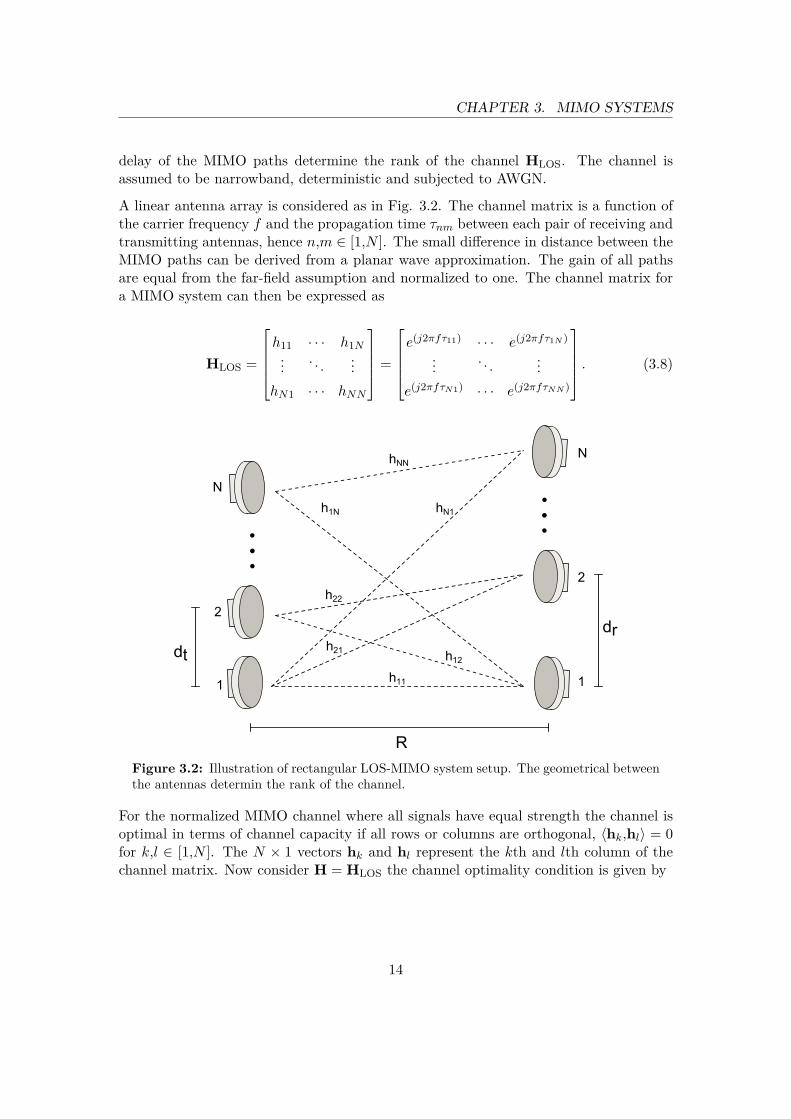
delay of the MIMO paths determine the rank of the channel HLOS. The channel isassumed to be narrowband, deterministic and subjected to AWGN.
A linear antenna array is considered as in Fig. 3.2. The channel matrix is a function ofthe carrier frequency f and the propagation time τnm between each pair of receiving andtransmitting antennas, hence n,m ∈ [1,N ]. The small difference in distance between theMIMO paths can be derived from a planar wave approximation. The gain of all pathsare equal from the far-field assumption and normalized to one. The channel matrix fora MIMO system can then be expressed as
HLOS =
h11 · · · h1N... . . . ...
hN1 · · · hNN
=
e(j2πfτ11) · · · e(j2πfτ1N )
... . . . ...e(j2πfτN1) · · · e(j2πfτNN )
. (3.8)
R
dt
dr
h11
h21
hN1
hNN
h12
h22
h1N
1
2
N
2
1
N
Figure 3.2: Illustration of rectangular LOS-MIMO system setup. The geometrical betweenthe antennas determin the rank of the channel.
For the normalized MIMO channel where all signals have equal strength the channel isoptimal in terms of channel capacity if all rows or columns are orthogonal, 〈hk,hl〉 = 0for k,l ∈ [1,N ]. The N × 1 vectors hk and hl represent the kth and lth column of thechannel matrix. Now consider H = HLOS the channel optimality condition is given by
14

CHAPTER 3. MIMO SYSTEMS
〈hk,hl〉 =N∑n=1
e(j2πf [τnk−τnl])
=N∑n=1
e(j2πλ
[rnk−rnl])
=N∑n=1
e(j2π[∠hnk−∠hnl]) = 0
(3.9)
where rnm is the geometrical distance from the mth transmitting antenna to the nthreceiving antenna, λ is the wavelength and ∠ is the angle operation. For a linear antennaarray, the optimality condition can easily be satisfied by a careful deployment. Thedistances rnm are given from the geometrical deployment and can be calculated from
rnm =√R2 + (ndr −mdt)2 ≈ R
(1 + (ndr −mdt)2
2R2
)= −nmdrdt
R+ n2d2
r −m2d2t
2R +R
(3.10)
where dt and dr are the antenna separation along a common axis normal to the hopdirection for the transmitter respective receiver and R is the hop length. Since d << Rthe distances can be approximated from the first order Taylor expansion. The pathdifference between antenna pairs is given by
rnk − rnl = (l − k)ndrdtR
+(k2 − l2
)d2t
2R . (3.11)
The second term (k2−l2)d2t
R only introduce a common phase shift which does not changethe orthogonality. This gives the resulting condition
〈hk,hl〉 =N∑n=1
e(j2π dtdr
λR(l−k)n
)= 0. (3.12)
By solving this equation subjected to the antenna separation distances it yields thesolution corresponding to the smallest separations as
dtdr = λR
N. (3.13)
So far the antenna array setup has been assumed to be parallel but the idea can easily beextended to non-rectangular setup. It was shown by [4] that every linear array setup can
15

CHAPTER 3. MIMO SYSTEMS
be projected on virtual parallel array for which the given optimality expression (3.13) isvalid. For a linear array, the optimality condition of (3.12) can be simplified in terms ofdeployment specific parameters to give the the deployment number η as in
η =
√dtdrλR
N. (3.14)
The channel deployment is optimal if η = 1 and a sub-optimal deployment will result inreduced channel capacity.
3.2.1 Alternative Optimality Conditions
In the case of 2× 2-MIMO system the capacity optimality condition of the channel canbe be related to the relative phase differences of the MIMO paths as in
∆θ = (∠h11 − ∠h12) + (∠h21 − ∠h22)− π (3.15)
where we introduce ∆θ as the MIMO phase. The expression is related to the orthogo-nality conditions in (3.9) by
〈h1,h2〉 = e(j2π[∠h11−∠h12]) + e(j2π[∠h21−∠h22]) = 0. (3.16)
The MIMO phase ∆θ is introduced as a parameter to measure optimal deploymentconditions and channel orthogonality in real systems. Later it is also used to measureuncorrelated phase variations of the MIMO paths during channel fading. In terms ofdeployment parameters, ∆θ becomes (3.17)
∆θ = 2πdtdrλR− π (3.17)
where the optimal value is given by ∆θOpt = 0.
3.3 Performance Measures
A various number of parameters can be used to characterize the performance of a MIMOsystem, such as channel capacity and outage probability. Channel capacity is a wellstudied limit and a widely used measure to analyse fundamental data rate limit of asystem. Outage probability is defined for a specific system as the probability that atransmission over the channel is not possible. However most practical systems operatebelow the theoretical limits due to hardware limitations, receiver complexity and channel
16

CHAPTER 3. MIMO SYSTEMS
variations. Most systems are limited by power and therefore system penalty γ is alsointroduced in this section, as an equivalent to fade attenuation of SISO systems. Thesystem penalty can also be used to define outage probabilities,
3.3.1 Capacity
Ergodic Capacity of the SVD-MIMO system with full CSI and parallel decompositionof the MIMO channel is given by
C = E[log2 det(IN + P
N0NHQH∗)
][bits/s/Hz]. (3.18)
The capacity of a ZF-MIMO receiver is given by
C = E[N∑k=1
log2
(1 + P/N
N0‖bk‖2)]
[bits/s/Hz]. (3.19)
as the sum of the capacity of the output signal streams [6]. The operator E representsthe expected value, det(·) is the determinant, H is the N × N channel matrix, IN isthe N × N identity matrix, P is the total transmitted power, N0 is the noise spectraldensity and Q denotes the signal covariance given by parallel channel decomposition andwater-filling power allocation as Q = VSV∗ [6]. In addition, ‖ · ‖ is the Euclidean norm.The vector bk is the kth row of the receiver matrix B.
The ergodic capacity is given from the time average of the instantaneous capacity. Ca-pacity is a good measure for random fast varying channels. However the measure is notappropriate for determining the quality or outage probability of a random channel thatare caused by fast deviation from the average signal level. For narrow-band channelthe ergodic capacity means the expected time averaged capacity. For a slow-varying ordeterministic channel ergodic and instantaneous capacity are equal. A common con-straint in MIMO systems is the absence of channel state information at the transmitter(CSIT). A capacity optimal transmission is then achieved by allocating equal power oneach spatial stream which gives the covariance matrix Q = I [8]. The capacity is givenby
C = E[log2 det(I + P
N0NHH∗)
][bits/s/Hz]. (3.20)
3.3.2 System Penalty
Microwave links are often associated with a fade margin wherefore a larger fade willresult in a system breakdown. While a fade margin cannot directly be applied on a
17
CHAPTER 3. MIMO SYSTEMS
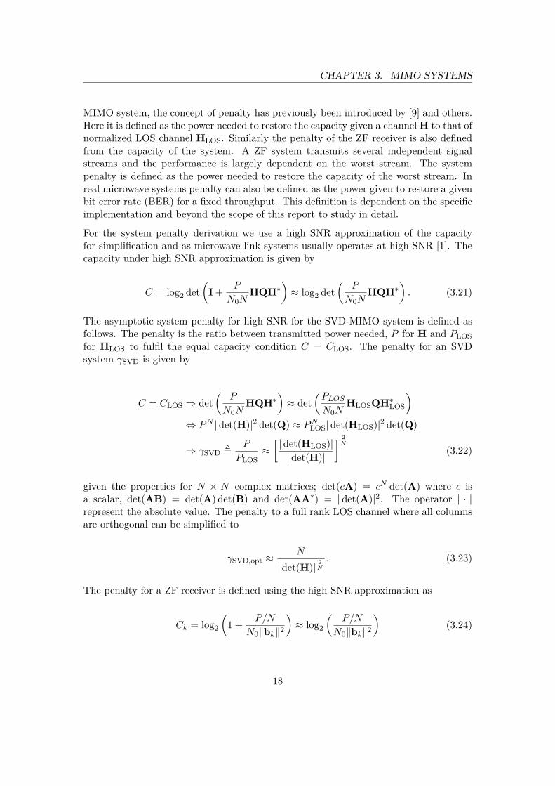
MIMO system, the concept of penalty has previously been introduced by [9] and others.Here it is defined as the power needed to restore the capacity given a channel H to that ofnormalized LOS channel HLOS. Similarly the penalty of the ZF receiver is also definedfrom the capacity of the system. A ZF system transmits several independent signalstreams and the performance is largely dependent on the worst stream. The systempenalty is defined as the power needed to restore the capacity of the worst stream. Inreal microwave systems penalty can also be defined as the power given to restore a givenbit error rate (BER) for a fixed throughput. This definition is dependent on the specificimplementation and beyond the scope of this report to study in detail.
For the system penalty derivation we use a high SNR approximation of the capacityfor simplification and as microwave link systems usually operates at high SNR [1]. Thecapacity under high SNR approximation is given by
C = log2 det(
I + P
N0NHQH∗
)≈ log2 det
(P
N0NHQH∗
). (3.21)
The asymptotic system penalty for high SNR for the SVD-MIMO system is defined asfollows. The penalty is the ratio between transmitted power needed, P for H and PLOSfor HLOS to fulfil the equal capacity condition C = CLOS. The penalty for an SVDsystem γSVD is given by
C = CLOS ⇒ det(
P
N0NHQH∗
)≈ det
(PLOSN0N
HLOSQH∗LOS
)⇔ PN |det(H)|2 det(Q) ≈ PNLOS| det(HLOS)|2 det(Q)
⇒ γSVD ,P
PLOS≈[ |det(HLOS)||det(H)|
] 2N
(3.22)
given the properties for N × N complex matrices; det(cA) = cN det(A) where c isa scalar, det(AB) = det(A) det(B) and det(AA∗) = | det(A)|2. The operator | · |represent the absolute value. The penalty to a full rank LOS channel where all columnsare orthogonal can be simplified to
γSVD,opt ≈N
|det(H)|2N
. (3.23)
The penalty for a ZF receiver is defined using the high SNR approximation as
Ck = log2
(1 + P/N
N0‖bk‖2)≈ log2
(P/N
N0‖bk‖2)
(3.24)
18
CHAPTER 3. MIMO SYSTEMS
where Ck is the capacity of the signal stream transmitted from the kth antenna, bk isthe kth row of ZF receiver matrix B given the channel H and k ∈ [1,N ]. The penaltyfor the ZF system γZF is defined as the power needed to restore the capacity, mink Ck,of the worst stream given H to that of the worst stream capacity, mink CLOS,k, of HLOS.This is expressed as
minkCk = min
kCLOS,k ⇒
P/N
N0 maxk ‖bk‖2≈ PLOS/N
N0 maxk ‖bLOS,k‖2
⇒ γZF ,P
PLOS≈ maxk ‖bk‖2
maxk ‖bLOS,k‖2. (3.25)
Again, the penalty to a full rank LOS channel where all columns are orthogonal can besimplified to
γZF,opt = N maxk‖bk‖2. (3.26)
Outage: One of the most important properties of a microwave link is outage probability.The outage for a given system is here defined as the probability of a penalty largerthan a penalty threshold. The penalty threshold is here related to the lowest acceptablecapacity or worst stream capacity depending on the receiver structure. The outageprobability is given by
Pout = Pr (γ > γthr) (3.27)
3.3.3 Capacity and System Penalty of Line-of-Sight MIMO systems
With the derived deployment number η for the channel HLOS (3.8) where all elementshave unit power, it is straight forward to calculate the capacity and system penalty forany linear array deployment, given hop-length, antenna separation and frequency. Froma design point-of-view it is interesting to see how the capacity and penalty are affectedfor non-optimal antenna separation and η 6= 1. For an easy deployment of the system,it is most often convenient to keep the separation as small as possible. For 2× 2 MIMOsystem it is possible to derive closed forms expressions for the deployment penalty withrespect to η in LOS channels. A simplified expression of (3.23) for a 2× 2 SVD-MIMOsystem in a normalized LOS channel (3.8) is given by
γSVD,2×2,deployment ≈∣∣∣∣sin(π2 η2
)∣∣∣∣−1. (3.28)
It can also be shown that a equivalent expression for a ZF-MIMO system derived fromderived from (3.26) is given by
19

CHAPTER 3. MIMO SYSTEMS
γZF,2×2,deployment =∣∣∣∣sin(π2 η2
)∣∣∣∣−2. (3.29)
Fig. 3.3a shows the variation of the penalty from (3.28) and (3.29), given the deploymentnumber η. For this case, η is equal to the ratio between the actual antenna separation dand optimal antenna separation dopt as η = d/dopt. One can show that for a 2× 2 LOS-MIMO system, the penalty can also be related to the MIMO phase ∆θ and equivalentlya MIMO phase penalty.
Since the expression of η involves the product of the antenna separations at both trans-mitter and receiver, it is possible to alter dt and dr individually. For an intuitive un-derstanding of sensitivity for deployment penalty, the penalty is plotted against both dtand dr in Fig. 3.4. for the ZF-MIMO system. As seen, relatively big changes for dt anddr can be allowed at a small penalty.
1 0.8 0.6 0.4 0.2 00
10
20
30
40
50
Dep
loymen
tpen
alty[dB]
Deployment number, η
ZF-MIMOSVD-MIMO
(a) The system penalty against η.
1 0.8 0.6 0.4 0.2 00
5
10
15
Cap
acity[bits/s/Hz]
Deployment number, η
ZF-MIMOSVD-MIMO
(b) The capacity against η at SNR=20dB
Figure 3.3: The system penalty and capacity for both 2 × 2 ZF-MIMO and SVD-MIMOsystem plotted against the deployment number η.
It is seen from Fig. 3.3 that for η > 0.7 the capacity loss is small and the penalty forboth systems is kept under γZF < 3 dB. When η = 1 it can be showed that the capacityof both systems is given by
Cmax = N log2
(1 + P
N0
). (3.30)
Given a total transmitted power constrain P the capacity is related to that of a SISOsystem multiplied with the number of spatial streams, N . As the separation decreasesthe capacity is reduced and penalty increases for both systems. The signal subspaceswill no longer be orthogonal which will cause interference between the spatial streams.When η = 0, HLOS becomes of rank 1 and will only support one spatial stream. For the
20

CHAPTER 3. MIMO SYSTEMS
2
2
2
4
4
4
4
6
6
6
6
8
8
8
10
10
2
12
4
14
6 8
16
10 12
18
14
dr/dopt
dt/dopt
0.4 0.6 0.8 1 1.2 1.4
0.4
0.6
0.8
1
1.2
1.4
2
4
6
8
10
12
14
16
18
20
Figure 3.4: System penalty [dB] for a 2×2 ZF-MIMO system against sub-optimal antennaseparation.
SVD-MIMO system, the capacity approaches that of a SISO system but with additionalarray gain from both the transmitter and receiver as
Cmin = log2
(1 +N2 P
N0
). (3.31)
However, for the ZF-MIMO system the capacity approaches zero since the channel onlywill support a single stream and interference cancellation is not possible. The penaltytherefore approaches infinity.
3.4 Wideband MIMO Systems
A system is considered wideband if the mean delay spread of the signal τm is smaller thatthe symbol time Ts. In time domain this will result in symbol dispersion and thus inter-symbol-interference (ISI). In the frequency domain it results in a non-flat spectrum. Atthe receiver this requires additional functions to manage the problem. The most commontechnique is called equalizing for which the name implies the spectrum is equalized andISI is removed. The operation can be performed in both time and frequency domain.
21
CHAPTER 3. MIMO SYSTEMS
3.4.1 Performance
The ergodic capacity of a wide band MIMO system is given by maximizing the rate byallocate transmitted power over both spatial and frequency dimensions as in
C = E[N∑n=1
∫log2
(1 + Psn(f)
NN0dn(f)2
)df]
(3.32)
where si(f) represent the power allocated to the ith transmitted signal at frequencyf and di(f) is the singular value of the channel matrix H(f) at frequency f . Eachspatial frequency selective channel can be seen as set of flat-fading sub-channels. Thenthe capacity is the sum of the capacity in the sub-channels subjected to a total powerconstraint. The optimal power allocation given CSIT is achieved with water-filling andequal allocation if CSIT is not available [6, 8]. The solution to the water-filling approachis given by solving
sn(f) =(ξ − 1
N0dn(f)2
)+,N∑n=1
∫sn(f)df ≤ N. (3.33)
where (·)+ is zero if its argument is negative. For an unknown channel at the transmitter(no-CSIT) the capacity is given by
C = E[N∑n=1
∫log2
(1 + P
NN0dn(f)2
)df]. (3.34)
The penalty for a wide band system can be defined as for the narrowband system, asthe power needed to restore capacity. However describing the penalty analytically in thesame way as in the narrowband channel is intractable.
3.5 Summary of Capacity and Penalty Expressions
Some important capacity expression used in this report are summarized in Tab. 3.1while penalty expressions are summarized in Tab. 3.2.
22

CHAPTER 3. MIMO SYSTEMS
Table 3.1: Summary of capacity expressions in narrowband MIMO systems
Capacity description ExpressionErgodic, SVD-MIMO C = E
[log2 det(IN + P
N0NHQH∗)
](3.18)
Ergodic, ZF-MIMO C = E[∑N
k=1 log2
(1 + P/N
N0‖bk‖2
)](3.19)
Optimal, full rank LOS channel (3.9) C = N log2
(1 + P
N0
)(3.30)
Table 3.2: Summary of asymptotic system penalty expressions for high SNR to an optimalLOS channel.
Description ExpressionSVD system penalty γSVD,opt ≈ N
| det(H)|2N
ZF system penalty γZF,opt = N maxk ‖bk‖2
2× 2 SVD deployment penalty γSVD,2×2,deployment ≈∣∣sin (π2 η2)∣∣−1
2× 2 ZF deployment penalty γZF,2×2,deployment =∣∣sin (π2 η2)∣∣−2
23
4Microwave Propagation
In this chapter we will present a theoretical overview of microwave propagation. We willalso explain the most important phenomenas that contribute to the fading on microwavelinks.
For any given wireless link the signal will experience various propagation losses includingthe free-space loss. The channel between the two terminals can be considered as arandom medium affecting the signal and hence the performance of the link. For alonger hop, the signal will pass through more random media and be more affected byrandom changes. This may cause big degradation in the performance. Physical effectsare generally grouped into two different categories; precipitation and clear-air effects.precipitation effects are attenuation due to rain, fog and snow. In this report, clear-air effects is referred to as refractive fading effects and are caused by changes in therefractive index in the atmosphere. Changes in the refractive index will cause the ray orwave front to bend and diverge from the nominal path.
Rain and refractive fading are usually considered as independent events [2] and theseverity of the fading is both dependent on the frequency and the hop length. Thefrequency used in most microwave systems ranges typically from 4 to 38GHz mainlydepending on hop-length and available spectrum [1]. As a rule of thumb microwave linksare often categorized in short-haul (0 to 15km), medium-haul (15-30km) and long-haul(30-150km) installations. Long-haul links often operate at lower frequencies between4-13GHz as those are less attenuated by rain. But longer hop-lengths also increase theprobability for refractive fading. Short-haul links usually do not suffer from refractivefading but are instead more sensitive to rain fading because higher frequencies are usuallyused. Higher frequencies are usually preferred due to available spectrum and benefits ofsmaller antennas with larger directivity. As a result short-haul links are usually limitedby rain while long-haul links are limited by refractive fading. Recently, links operating
24

CHAPTER 4. MICROWAVE PROPAGATION
in the E-band (70-90GHz) or even higher frequencies have been investigated. This allowsfor short but high capacity links since the available spectrum is large.
Both rain and refractive fading depend strongly on climatic factors and both effects oftenneeds to be taken into account when planning a link. This section will in more detaildescribe rain and refractive fading.
4.1 Rain fading
It is well known that rain will attenuate the overall signal power level of a microwave link.This is mainly because of scatter caused by the rain droplets but also due to dielectriclosses. The loss is related to the rain rate and the relation between droplet size andthe wavelength. In general, shorter wavelengths are more attenuated and for frequenciesbelow 5GHz the attenuation can usually be ignored. There is also a small differencein attenuation between horizontal and vertical polarized signal due to the slightly flatshape of water droplets caused by the wind resistance. Fig. 4.1 shows the attenuationcaused by rain against the frequency for different rain rates. A well-known empiricalformula of rain attenuation from ITU is given as
γR = kRαrain (4.1)
where Rrain is the rain rate [mm/h]. The coefficients k and α are frequency and polar-ization dependent parameters which can be calculated or given from tables provided byITU [10].
101
102
0
5
10
15
20
25
30
35
40
45
Frequency [GHz]
Attenuation[dB/k
m]
5mm/h25mm/h50mm/h100mm/h150mm/h
Figure 4.1: Rain attenuation for horizontal polarization against frequency for differentrain rates.
25

CHAPTER 4. MICROWAVE PROPAGATION
Another effect caused by rain is depolarization which can give problems to systems usingdual polarizations to transmit independent signals. Polarization distortions affect thesystem’s ability to separate the signals at the receiver based on their polarization. Inaddition, rain may also change the properties of reflecting surfaces. A wet surface oftenhas increased conductivity which can increase reflections and scatter. It has been shownthat links partly obstructed by vegetation can experience increased scatter during rain[11].
4.2 Refractive Fading
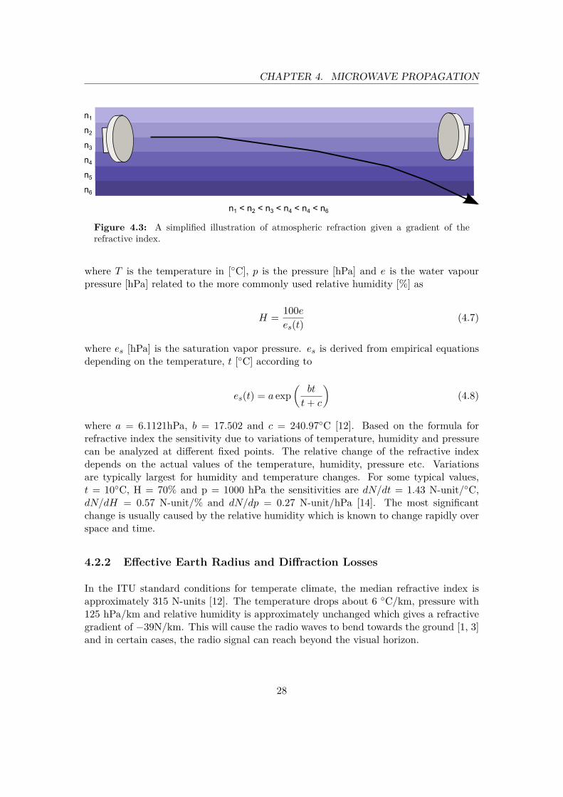
The atmosphere is not a homogeneous media as often approximated. Properties, suchas temperature, humidity and pressure of the air will change over both space and time.These properties will also change the refractive properties of the atmosphere. Refractivefading can be characterized into several different effects with different fading properties.In this section we present the most significant effects such as diffraction loss, defocus-ing/ducting and multipath fading, also presented in Tab. 4.1.
Table 4.1: Overview of refractive fading effects.
Slow/frequency flat Fast/frequency selectiveDefocusing Mulitpath
Effective earth radius and diffraction
Defocusing/ducting, diffraction and rain fading are usually considered as slow and fre-quency flat fading events i.e., they usually lasts longer than 10 seconds and affect outage.Multipath fading on the other hand, usually cause fast and frequency selective fading,affecting the short term performance [1]. Multipath fading can last over a few secondsor less. As will be seen, refractive effects are generally dependent on both propagationdistance and frequency.
4.2.1 Refractive index
Wave propagation in any media such as air or glass is characterized by the refractiveindex of the constant defined by
n = c
v(4.2)
where c is the propagation speed of light in vacuum and v is the propagation speed inthe medium. The refractive index of vacuum is therefore given by n=1. There are manyphenomenas related to the refractive index and the wave nature of radio signals. Most
26
CHAPTER 4. MICROWAVE PROPAGATION
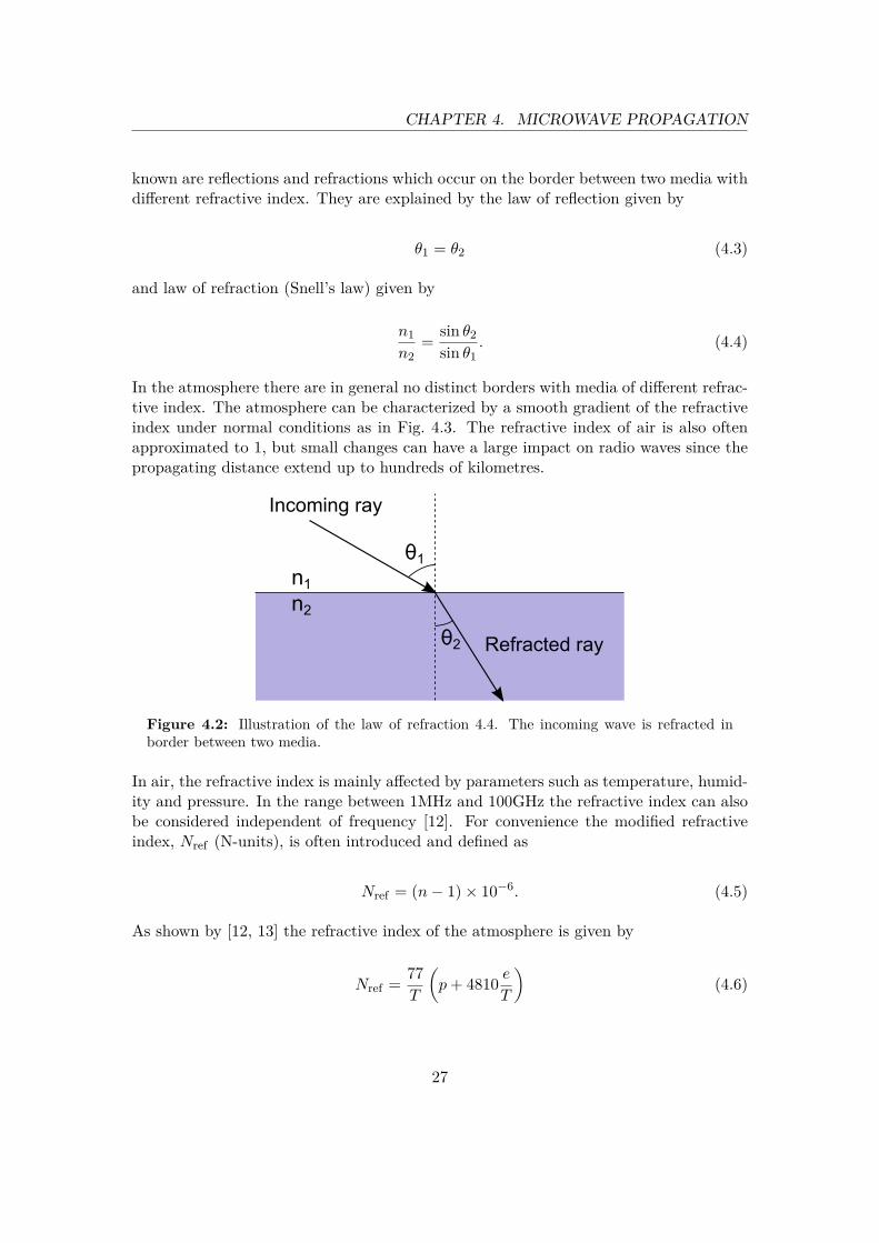
known are reflections and refractions which occur on the border between two media withdifferent refractive index. They are explained by the law of reflection given by
θ1 = θ2 (4.3)
and law of refraction (Snell’s law) given by
n1n2
= sin θ2sin θ1
. (4.4)
In the atmosphere there are in general no distinct borders with media of different refrac-tive index. The atmosphere can be characterized by a smooth gradient of the refractiveindex under normal conditions as in Fig. 4.3. The refractive index of air is also oftenapproximated to 1, but small changes can have a large impact on radio waves since thepropagating distance extend up to hundreds of kilometres.
θ1
θ2
Incoming ray
Refracted ray
n1
n2
Figure 4.2: Illustration of the law of refraction 4.4. The incoming wave is refracted inborder between two media.
In air, the refractive index is mainly affected by parameters such as temperature, humid-ity and pressure. In the range between 1MHz and 100GHz the refractive index can alsobe considered independent of frequency [12]. For convenience the modified refractiveindex, Nref (N-units), is often introduced and defined as
Nref = (n− 1)× 10−6. (4.5)
As shown by [12, 13] the refractive index of the atmosphere is given by
Nref = 77T
(p+ 4810 e
T
)(4.6)
27
CHAPTER 4. MICROWAVE PROPAGATION
n6
n5
n1
n2
n3
n4
n1 < n2 < n3 < n4 < n4 < n6
Figure 4.3: A simplified illustration of atmospheric refraction given a gradient of therefractive index.
where T is the temperature in [◦C], p is the pressure [hPa] and e is the water vapourpressure [hPa] related to the more commonly used relative humidity [%] as
H = 100ees(t)
(4.7)
where es [hPa] is the saturation vapor pressure. es is derived from empirical equationsdepending on the temperature, t [◦C] according to
es(t) = a exp(
bt
t+ c
)(4.8)
where a = 6.1121hPa, b = 17.502 and c = 240.97◦C [12]. Based on the formula forrefractive index the sensitivity due to variations of temperature, humidity and pressurecan be analyzed at different fixed points. The relative change of the refractive indexdepends on the actual values of the temperature, humidity, pressure etc. Variationsare typically largest for humidity and temperature changes. For some typical values,t = 10◦C, H = 70% and p = 1000 hPa the sensitivities are dN/dt = 1.43 N-unit/◦C,dN/dH = 0.57 N-unit/% and dN/dp = 0.27 N-unit/hPa [14]. The most significantchange is usually caused by the relative humidity which is known to change rapidly overspace and time.
4.2.2 Effective Earth Radius and Diffraction Losses
In the ITU standard conditions for temperate climate, the median refractive index isapproximately 315 N-units [12]. The temperature drops about 6 ◦C/km, pressure with125 hPa/km and relative humidity is approximately unchanged which gives a refractivegradient of −39N/km. This will cause the radio waves to bend towards the ground [1, 3]and in certain cases, the radio signal can reach beyond the visual horizon.
28

CHAPTER 4. MICROWAVE PROPAGATION
Another view of the effect of a changing refractive index is given by the concept ofeffective earth radius. If the refractive gradient is considered constant along the paththe effective earth radius means to compensate for the ray-bending. Example, if the raysbends just as much as the real earth curvature the effective earth would look flat for theradio waves, and the effective earth radius would be infinite. The effective earth can becharacterized by the so called kearth-factor given by
kearth = 1R+ δN
δh 10−6 (4.9)
where kearth = 1 represent the actual radius. It is easy to verify that the standardgradient of -39 N-units/km gives the widely used k value of approximately k = 4/3.A refractive gradient of -157 N-units/km gives k = ±∞. Under such conditions or forsmaller gradients the radio signals can travel far beyond the visual horizon with littleloss. This is referred as super refractive conditions or ducting. The effective earth radiuswill be negative which implies that the signal will bend strongly towards the ground.Gradients larger than the normal conditions of -39N/km is referred as sub-refractiveconditions. Under such conditions the effective earth radius will appear small and thesignal will bend upwards.
The effective earth radius is often used to calculate the needed path clearance of a link.The path clearance is defined as the distance from the geometrical line-of-sight pathtrajectory to the closest object or the ground. As the effective earth radius decreasesthe ground or any object will appear higher. This effect is visualized in Fig. 4.4 wherethe effective ground is shown for three different kearth-values.
0 5 10 15 20 250
20
40
60
80
100
Distance [km]
Elevation
[m]
k = 0.6k = 1.3k = inf.
Figure 4.4: Example of effective ground height for some effective earth radius values. Theellipse shows the first Fresnel zone where obstruction losses can be significant.
29
CHAPTER 4. MICROWAVE PROPAGATION
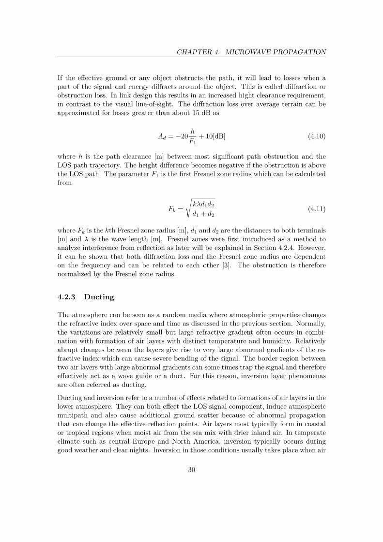
If the effective ground or any object obstructs the path, it will lead to losses when apart of the signal and energy diffracts around the object. This is called diffraction orobstruction loss. In link design this results in an increased hight clearance requirement,in contrast to the visual line-of-sight. The diffraction loss over average terrain can beapproximated for losses greater than about 15 dB as
Ad = −20 hF1
+ 10[dB] (4.10)
where h is the path clearance [m] between most significant path obstruction and theLOS path trajectory. The height difference becomes negative if the obstruction is abovethe LOS path. The parameter F1 is the first Fresnel zone radius which can be calculatedfrom
Fk =√kλd1d2d1 + d2
(4.11)
where Fk is the kth Fresnel zone radius [m], d1 and d2 are the distances to both terminals[m] and λ is the wave length [m]. Fresnel zones were first introduced as a method toanalyze interference from reflection as later will be explained in Section 4.2.4. However,it can be shown that both diffraction loss and the Fresnel zone radius are dependenton the frequency and can be related to each other [3]. The obstruction is thereforenormalized by the Fresnel zone radius.
4.2.3 Ducting
The atmosphere can be seen as a random media where atmospheric properties changesthe refractive index over space and time as discussed in the previous section. Normally,the variations are relatively small but large refractive gradient often occurs in combi-nation with formation of air layers with distinct temperature and humidity. Relativelyabrupt changes between the layers give rise to very large abnormal gradients of the re-fractive index which can cause severe bending of the signal. The border region betweentwo air layers with large abnormal gradients can some times trap the signal and thereforeeffectively act as a wave guide or a duct. For this reason, inversion layer phenomenasare often referred as ducting.
Ducting and inversion refer to a number of effects related to formations of air layers in thelower atmosphere. They can both effect the LOS signal component, induce atmosphericmultipath and also cause additional ground scatter because of abnormal propagationthat can change the effective reflection points. Air layers most typically form in coastalor tropical regions when moist air from the sea mix with drier inland air. In temperateclimate such as central Europe and North America, inversion typically occurs duringgood weather and clear nights. Inversion in those conditions usually takes place when air
30

CHAPTER 4. MICROWAVE PROPAGATION
close to the ground cools off quicker than the air above which raises the relative humidityand creates a large negative gradient. Layers can form both close to the ground, creatingsurface ducts or higher from the ground, creating elevated ducts. Most severe conditionsare usually when the duct forms in the same height as line-of-sight. When describingthe properties of ducts and the profile of the refractive index, the modified refractivityunit Mref is often used [12]. The M -unit is given from
Mref = Nref + 157h (4.12)
where h is the height over the earth’s surface in km. The M-units becomes smallerthan the initial value when ducting condition is fulfilled (dN/dh < −157 N-units/km).This property makes the measure Mref useful when analysing ducts. Therefore, anotherpractical indicator of ducting events is the so called M-profiles [12, 14]. Fig. 4.5 depictssome examples of typical ducting profiles i.e., elevated and surface ducts. The profilesare given by [14]
N(h) = N0 +GNh+ dN
2 tanh 2.96(h− h0)dh
(4.13)
where h is the elevation [m], N0 is the refractive index [N-unit] at h = 0, GN is thenominal refractive gradient [N-unit/m], h0 is the elevation of the duct [m], dN is theduct depth [N-units] and dh is the duct width [m].
290 300 310 3200
50
100
150
Refractivity [N,M-units]
Elevation[m
]
Standard Conditions
M−unitsN−units
(a) Standard gradient, -39N-units/km
280 300 3200
50
100
150
Refractivity [N,M-units]
Elevation[m
]
Elevated Duct
M−unitsN−units
(b) Elevated duct, h0 =80m, δh = 40m, δN = −20
280 290 300 3100
50
100
150
Refractivity [N,M-units]
Elevation[m
]
Surface Duct
M−unitsN−units
(c) Surface duct h0 =0m, δh = 40m, δN = −20
Figure 4.5: Example of two duct profiles and the standard gradient.
Propagation through ducts, inversions or other abnormal change of the refractive indexcan have an adverse effect on the received signal. In agreement with performance pre-diction methods [2, 15] and ray-tracing simulations, the effects are enhanced with bothhop length and frequency. A longer hops means the signal will likely propagate longerthrough abnormal refractive media and deviate more from the nominal propagation.This increases probability of focusing and defocusing phenomenas. For multipath thedifference in distance between the line-of-sight and the multipath component may alsoincrease, which increases the probability of destructive interference.
31

CHAPTER 4. MICROWAVE PROPAGATION
The effect of signal propagation through an elevated duct over 10km is simulated withray-tracing and shown in Fig. 4.6a. In the figure, it seen that the rays of the signalbend little from nominal conditions. The distance axis represents the distance alongthe Earth’s surface, wherefore the rays will appear to bend upwards from the ground.Reflections at Earth’s surface have been added to visualize presence of reflections. Fig.4.6b shows the same scenario over 30km and as seen the ray-bending becomes muchmore severe. The figures also visualize some typical effects of focusing/defocusing wherethe rays combine or diverge.
Distance [km]
Elevation
[m]
1 2 3 4 5 6 7 8 9 10
30
60
90
120
(a) Propagation over 10km.Distance [km]
Elevation
[m]
3 6 9 12 15 18 21 24 27 30
30
60
90
120
(b) Propagation over 30km.
Figure 4.6: Example of two ray tracing simulation through an elevated duct 4.13 withdifferent propagation distance.
Distance [km]
Elevation
[m]
2 4 6 8 10 12 14 16 18 20
30
60
90
120
(a) Horizontal propagationDistance [km]
Elevation
[m]
2 4 6 8 10 12 14 16 18 20
30
60
90
120
(b) Inclined propagation
Figure 4.7: Example of a horizontal and inclined propagation through a duct over 20 km.
The effects are frequency dependent, especially when multipath or scatter is present.Higher frequencies usually increase probability of severe fading due to larger phase vari-ations of the multipath components. Another important aspect is the angle of arrival of
32

CHAPTER 4. MICROWAVE PROPAGATION
the signal through the duct. The impact of the angle of arrival is more severe for smallangles. An inclined path will make the signal propagate quickly through the horizontallayer without much effect as is illustrated in Fig. 4.7a. and 4.7b.
4.2.4 Multipath
Both atmospheric multipath and multipath from surface reflections are strongly relatedto ducting and abnormal propagation. Abnormal propagation can quickly change thedelay and distance of a multipath component. Mulitpath fading usually becomes moresevere in combination with strong ducting or defocusing events when the LOS componentis weaker than nominal conditions. The multipath components can become dominantwhich lead to a fast frequency selective fading [16, 17]. Multipath or scattered signalsare usually not desirable in LOS microwave links. Multipath can arise from strong(specular) reflection from flat surfaces or refractions in the atmosphere. Scattering isusually origins from multiple weak reflections from the ground and surrounding objects.
The received signal is dependent on the relative phase and amplitude between the mul-tipath and LOS component. The farther away the reflection occurs from the LOS paththe greater the difference in distance will be between the components. This conceptis generalized by Fresnel zones where the reflection on the border between such zonesresults in constructive (even zones) or destructive (odd zones) interference.
As mentioned earlier, variations of the effective earth radius and the propagation con-ditions may also change the effective reflection points. Multipath fading can thereforechange very quickly, in order of seconds or less [1, 3]. Generally, it is difficult to predictthe effect of scatter and non-specular reflections. For MIMO systems it is even harderto foresee the effects due to the several slightly separated MIMO paths as illustrated inFig. 4.8.
Figure 4.8: Illustration of refraction and reflection in LOS-MIMO system.
33

CHAPTER 4. MICROWAVE PROPAGATION
4.2.5 Electrical distance
The electrical distance is another important phenomena related to the refractive indexof the atmosphere. The electrical distance between two points can be expressed in theduration of travel τ , determined by the propagation speed v in (4.2) or directly in termsof the geometrical distance and refractive index. The electrical distance is given by
delectrical = nd (4.14)
where d is the geometrical propagation distance. For microwave frequencies even verysmall variations of the refractive index can lead to significant phase changes. This effecthas been measured by for example [18]. For a LOS-MIMO system, uncorrelated changesof the electrical distance may lead to additional fading and system penalty but it isbeyond the scope of this report to study this effect.
34

5Channel Models
In this Chapter we will present the ITU method to predict long term variations of amicrowave link channel. We will also present analytical channel models motivated bymeasurements in Chapter 6 to evaluate short term performance.
Many physical phenomenas are known to cause fading and affect performance of a link.The most significant ones were described in the previous section. There are differenttypes of channel models but it is possible to roughly divide them into two classes; phys-ical and analytical models [19]. In addition to channel models there exist several semi-empirical fading prediction methods such as the ITU methods. A prediction methodaims to predict the statistical outcome of the channel. A physical model aims to re-produce the actual propagation environment, from geometry to atmospheric conditions.A physical model can often be extensive and complex but also very accurate. Ana-lytical models aim to characterize the impulse response of the channel between each atransmitter and receiver pair. Analytical models often intend to characterize a channelsubjected to specific weather conditions. They are therefore useful to analyse systemsshort term performance. The empirical methods such as the ITU use both analyticalmodels and empirical data over weather and environmental conditions to predict a totalfading distribution over the whole year.
For a conventional Single-Input-Single-Output (SISO) link, there exists many channelmodels and methods to predict variations and statistics of the received power [1]. ITURec. P.530 [2] is considered as industry standard and provides a semi-empirical modelbased on comprehensive measurements. It is good for an initial planning purpose. Moredetailed models of short term fading have often resulted in analytical and propagationmotivated models. Depending on the complexity, these models can provide a moreaccurate reproduction of real channels [19].
Microwave MIMO channels differ from its SISO counterpart with several slightly spatially
35
CHAPTER 5. CHANNEL MODELS
separated paths. Since the separation is small and the signals propagate in common me-dia a high degree of correlation between the signals can be assumed. This is also shownfrom studies on microwave links with two or more spatially separated receives for diver-sity protection [2, 20, 21]. Some available studies have investigated amplitude correlationfor severe fading events but little is known about phase and amplitude correlations forany fade depth. The phase correlations are important because it can change the orthog-onality condition (3.9) of the channel and therefore increase the system penalty.
An important property of most microwave models is that the received power at deep fades(& 10dB) is assumed to follows Rayleigh statistics during refractive fading. This givesrise to a characteristic Rayleigh slope of 10dB-per-decade of the deep fade probabilities.This property has been extensively verified by measurements. Meanwhile, more shallowfades are often assumed to be log-normal or as in the case of the ITU-model follow anempirical distribution [3, 22, 23, 24].
In the following sections the ITU prediction methods will be described together withsome common analytical models applied on microwave links. Their properties, advan-tages and disadvantages will be explained. Later equivalent MIMO channel models willbe described.
5.1 Path-loss
Path-loss is the reduction of power density of an electromagnetic wave that propagatesthrough space. The loss is proportional to the propagation distance and is present toto any wireless communication system. Path-loss is one of the major components whenanalysing the link budget. For the case of LOS propagation through a homogeneousmedia and full clearance of the first Fresnel zone, the path-loss L is approximated withthe free-space loss calculated with Friis formula (5.1)
L = 20 log10
(4πdλ
)(5.1)
where d is the propagation distance and λ is the wave-length. The formula is derivedfrom the expansion of a spherical wave when d� λ e.g. far field condition.
5.2 ITU Method
The ITU method is often considered an industry standard of availability predictionmethods [1]. The model considers both rain and refractive fading. It also discussessome key design parameters as antenna height and clearance to reduce outage due todiffraction. The model is semi-empirical in the sense it heavily relies on measurements tofit the models. Rain end refractive fading are considered independent event by the ITU
36

CHAPTER 5. CHANNEL MODELS
method, which is divided to handle rain fading, refractive fading and frequency selectivedistortion separately. Multipath caused by refractive fading is generally considered tofast varying (< 10s) and affect performance while rain is slow varying (> 10s) and affectsoutage.
5.2.1 Rain Attenuation
The specific rain attenuation is described in section 4.1. The total rain attenuation ofthe link is given by the hop length and the specific attenuation for a specific rain rate.Statistical data for rain rates are often readily available which makes it straight forwardto predict attenuation caused by rain. However, the rain rate may vary along the hopand the ITU method compensates for this effect by calculating an effective rain distancefactor, reff given by
reff = 10.477d0.633R0.073α
0.01 f0.123 − 10.159(1− e−0.024d)(5.2)
where R0.01 is the rain rate exceeded 0.01% of the year and α is the same coefficientas from (4.1). The rain rate R0.01 together with the distance d and the effective raindistance factor reff is used to calculate the rain attenuation exceeded 0.01% of the year,
A0.01 = γRdreff (5.3)
where γR is the specific rain attenuation given for the rain rate exceeded 0.01% of theyear. The full method also provide formulas for other percentages of time [2].
5.2.2 Refractive fading
Refractive fading is known to be caused by many propagation effects but ITU providea method to calculate the total distribution of the fading. Multipath fading is believedto cause the 10dB-per-decade slope of the distribution, often under influence of othereffects such as defocusing [2, 16]. Here, the channel is assumed to be narrow-bandand the fading to be frequency-flat. Outage due to frequency selective fading are highlydependent on the specific receiver and is thereby handled separately by the ITU method.The ITU method assumes deep fades for a small percentage of time where the amplitudedistribution can be characterized by the Rayleigh distribution. The small percentage oftime pw that fade depth A [dB] is exceeded in the average worst month can be calculatedfrom:
pw(A) = p0 × 10(−A/10)[%] (5.4)
37
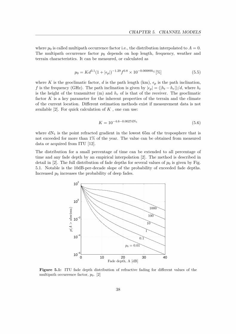
CHAPTER 5. CHANNEL MODELS
where p0 is called multipath occurrence factor i.e., the distribution interpolated to A = 0.The multipath occurrence factor p0 depends on hop length, frequency, weather andterrain characteristics. It can be measured, or calculated as
p0 = Kd3.1(1 + |εp|)−1.29f0.8 × 10−0.00089hL [%] (5.5)
where K is the geoclimatic factor, d is the path length (km), εp is the path inclination,f is the frequency (GHz). The path inclination is given by |εp| = (|ht−hr|)/d, where htis the height of the transmitter (m) and hr of is that of the receiver. The geoclimaticfactor K is a key parameter for the inherent properties of the terrain and the climateof the current location. Different estimation methods exist if measurement data is notavailable [2]. For quick calculation of K , one can use:
K = 10−4.6−0.0027dN1 (5.6)
where dN1 is the point refracted gradient in the lowest 65m of the troposphere that isnot exceeded for more than 1% of the year. The value can be obtained from measureddata or acquired from ITU [12].
The distribution for a small percentage of time can be extended to all percentage oftime and any fade depth by an empirical interpolation [2]. The method is described indetail in [2]. The full distribution of fade depths for several values of p0 is given by Fig.5.1. Notable is the 10dB-per-decade slope of the probability of exceeded fade depths.Increased p0 increases the probability of deep fades.
0 10 20 30 4010
−6
10−4
10−2
100
102
Fade depth, A [dB]
p(A
>ab
scissa)
p0 = 0.01
0.1
1
10
100
1000
Figure 5.1: ITU fade depth distribution of refractive fading for different values of themultipath occurrence factor, p0. [2]
38

CHAPTER 5. CHANNEL MODELS
5.2.3 Outage Due to Distortion
The main cause of signal distortion include multipath propagation that causes frequency-dependent, amplitude and phase variation [2, 22]. In digital systems such distortion ishandled by different types of equalizers. If the distortion itself generates an outage, itmight not help by increasing the fade margin. In this case, the ITU model predicts theoutage of such distortion using a so called signature method, where the systems abilityto handle in-band distortion is derived [2]. Currently, there is no equivalent signaturemethod for MIMO systems since the path correlation of the MIMO channel is not known.However, some simulations on specific cases of frequency selective channels have beenperformed by [9].
5.3 Analytical Models
A common analytical model describing SISO systems is the multi-ray model where thechannel is characterized by the statistics of each multipath components. However, MIMOchannels are often described by multivariate distribution to capture correlated fading be-tween the MIMO paths. In this section, an extension of the multi-ray model is proposedto cover the MIMO case by describing each channel component using multivariate ran-dom variable.
5.3.1 Multiple-path Models
The fading during refractive fading has often been found to be composed of several com-ponents [22, 23, 24, 25]. In particular the channel often contains a frequency-flat compo-nent from defocusing and other slow-varying effects, and also a fast-varying, frequency-selective component mainly caused by ground scatter [3, 16, 17]. Based on the aboveobservation, a propagation motivated multi-path model has been proposed given by
h =∑i
aie(j 2π
λτi). (5.7)
The multi-path model produces the channels impulse response for a limited time. Henceit does not provide any outage prediction for all the time but it is useful to in detail studythe performance of a systems under specific fading events. If needed, the probabilityof fading events can then be used to calculate the overall outage. In an extension ofthe multi-path model to cover MIMO cases, the single path component will be replacedby the MIMO channel component Hi. Each multipath MIMO channel represents areflection or scatter from the same area. For wide-band channel it is assumed that everyelement of the MIMO multipath component has the same delay, τi as (5.8)
39
CHAPTER 5. CHANNEL MODELS
H(f) =∑i
Hie(j2πfτ) (5.8)
when the separation between the antennas is relatively small. However in this report wehave focused on narrow-band systems where the delay is approximately zero.
5.3.2 Correlated Rician and Rayleigh Model
A very common analytical model in literature for LOS-propagation is the Rician channel[6, 19]. From our real-world measurements presented in Chapter 6 the Rician modelworks also well to model multipath fading. In this context the Rician channel can beseen as a special case of the general two-ray model used to model fast-varying effects.The Rician channel is given by
H =√
κ
1 + κHLOS +
√1
1 + κHNLOS (5.9)
where κ is the Rician factor, HLOS is the N ×N normalized deterministic channel. Asa result of small spatial separation between antennas, the elements of the NLOS N ×Nchannel component, HNLOS, are assumed to be correlated Gaussian distributed withequal mean and variance. A special case of the Rician channel with no significant staticdeterministic component is the Rayleigh channel given by
H = HNLOS. (5.10)
The distribution of HNLOS is given by [19, 26]
p(hNLOS) = 1πN2 det(ΣNLOS)
exp(−h∗NLOSΣ−1
NLOShNLOS)
(5.11)
where hNLOS = vec (HNLOS) and vec (·) is the vectorization operator, ΣNLOS is thecovariance matrix. ΣNLOS contains information of the correlation structure betweenthe paths. To be able to study MIMO path correlation, we define a simple correlationstructure and the correlation matrix to be
ΣNLOS = E[hNLOSh∗NLOS] =
1 ρ21 · · · ρN21
ρ12 1... . . .
ρ1N2 1
(5.12)
40

CHAPTER 5. CHANNEL MODELS
where all elements have equal correlation magnitude but correlation phases are specifiedby the LOS channel HLOS. This is motivated by the small spatial separation of theMIMO paths. Hence, the absolute values of the elements of ΣNLOS are given by |ρij | = ρwhere | · | is the absolute value. The correlation phases are given by ∠ρij = ∠hLOS,i −∠hLOS,j ∀i 6= j, |ρii| = 1 and ∠ρii = 0 where arg(·) is the argument function. Theelement hLOS,i is the ith element of the vector hLOS = vec (HLOS) and i,j ∈ [1,N2] Alower value of ρ leads to lower correlation between different paths in both phase andamplitude.
It has been shown by many studies that in severe events of refractive/multipath fadingthe channel can be characterized by Rayleigh fading. From our measurements presentedin Chapter 6 and earlier studies [19] we have seen that the Rician channel can be used tomodel multipath fading. For this reason the Rayleigh and the Rician channel will be usedin Chapter 7 later to analyse deep fading distributions and impact of path correlation.
41

6Measurements
In order to demonstrate a working LOS-MIMO system and to collect fading data, twomicrowave 2 × 2 LOS-MIMO test links were deployed at Ericsson’s site in Mölndal,Sweden. The channel fading data were collected to help understand and characterizeboth long and short term fading in a LOS-MIMO system.
Measurements from the systems were collected during 2012 and until June 2014. A sum-mary of the two links is listed in Tab. 6.1. The first link L1 is 5.3km long and it operatesat 8GHz, with horizontally separated antennas. The second link L2 is 1.3km long, andit operates at 32GHz, with vertical antenna separation. An overview of the geographicaldeployment is shown in Fig. 6.1. Both links are deployed close to optimal conditionsaccording to (3.14) and both links have full clearance and no obstruction within the firstFresnel zone. According to the ITU model the propagation can therefore be approxi-mated with free-space propagation. For the test links, the following parameters weremeasured and logged to characterize the channel fading to study atmospheric impact:
(i) Received power, PRX(ii) MIMO phase ∆θ (3.15)
In addition, meteorological data, such as wind speed, temperature, humidity, pressureand rain rate was measured at two 15m vertically separated weather stations at Ericsson’ssite. Apart from weather conditions these parameters can be used to calculate therefractive index of the atmosphere with (4.6) in Chapter 4. Two measuring pointscan not give a full picture of refractivity along the entire signal path. However, themeasurements from the two weather stations provide us with a useful estimation of thevertical variation of refractivity.
42

CHAPTER 6. MEASUREMENTS
Table 6.1: Link Setup Summary. (·) represent value for the second direction.
Link Sisjo link Sahlins linkLabel L1 L2Location 1 Ericsson EricssonLocation 2 Sisjon water tower Sahlins Terass buildingHop length (km) 5.314 1.355Frequency (GHz) 7.989 (8.299) 31.815 (32.627)Antenna separation Horizontal VerticalPolarization Horizontal VerticalDeployment number, η 1.003 (1.022) 0.989 (1.002)
Mölndal
Figure 6.1: Overview of the the geographical link deployment. L1 is represented by theblue arrow and L2 by the red arrow.
6.1 System Structure
The receivers used in the LOS-MIMO test links can be described as a correlation basedinterference cancelling receivers. A simplified receiver structure is presented by the blockdigram in Fig. 6.2. At the transmitter, two independent signal streams are transmittedby the two spatially separated antennas. The received signals are sampled and thereafterfed to an equalizer. RX1 and RX2 represent the received signal at the two receiving
43

CHAPTER 6. MEASUREMENTS
EQ
EQ CPT
B A
C
RX1
RX2
Figure 6.2: Receiver cancellation structure of the prototype receiver. The CPT blockrepresent the Carrier Phase Tracker
antennas in Fig. 6.2. The received signal at RX1 and RX2 then consist of a sum of thetwo transmitted signal streams. From the geometry of the deployment the received signalstreams are received at the antennas with independent phases. The received signals arethen scaled and rotated so the unwanted interference signal of RX1 and RX2 have equalpower and are shifted by 180◦, and therefore cancel each other out. The signal aftercancellation will consist of the sum of the wanted signal stream from RX1 and RX2.The process is visualized in Fig. 6.3.
90
90
0
0
-90
-90
Figure 6.3: Simple illustration of the signal cancellation process.
If the deployment optimality condition are met the wanted signal will have the samerelative phase and add constructively. The system will work even if the optimalitycondition does not hold. In such case, the wanted signal will not have the same phaseand therefore the combining cannot be optimal. Finally, the combined signal is rotatedand fed to the slicer. Simplified, the system is equivalent to the theoretical ZF-MIMOreceiver described in Section 3.1.2.
Two different methods to measure the MIMO phase are used. The first method is acorrelation based method used in the LOS-MIMO test links receivers described previ-ously. It is referred as the correlation method. The second method uses the relativephase difference between two sinusoid tones. The method is referred to as the sinusoid
44
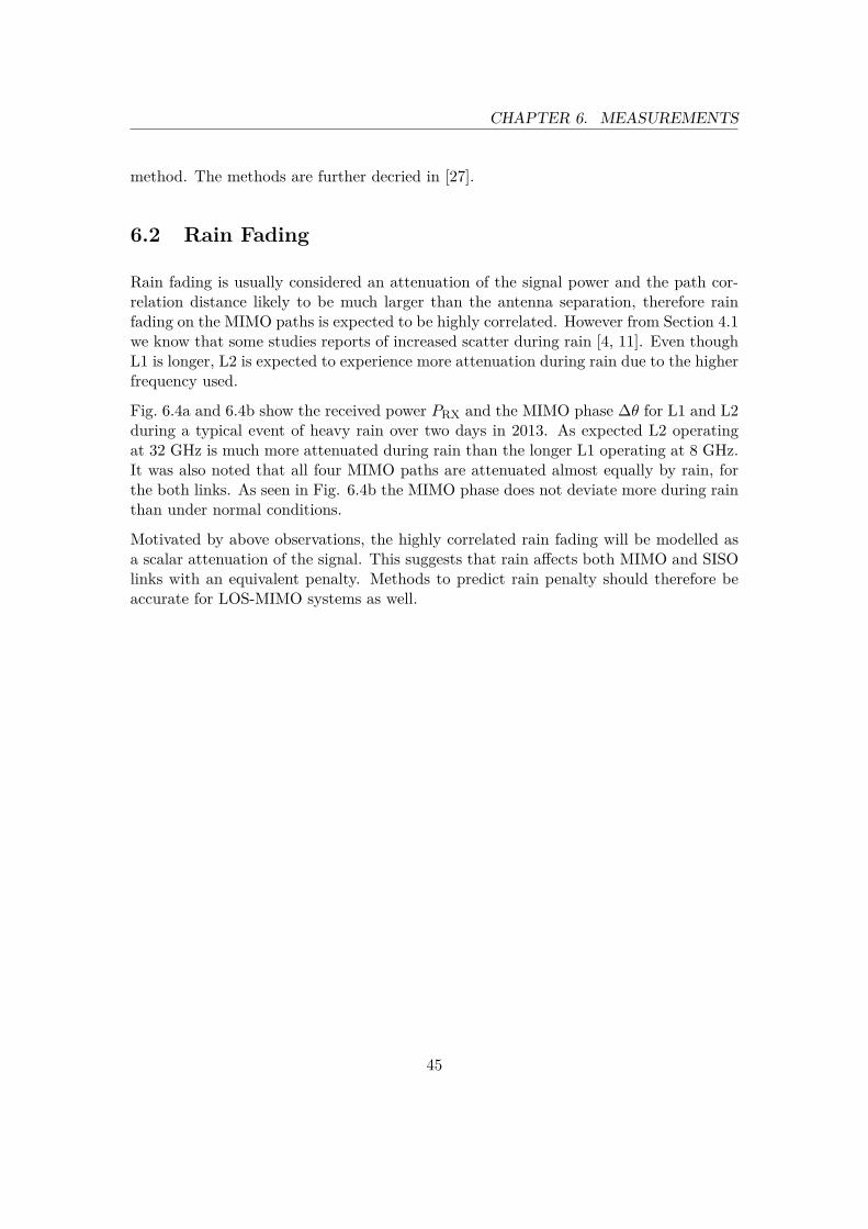
CHAPTER 6. MEASUREMENTS
method. The methods are further decried in [27].
6.2 Rain Fading
Rain fading is usually considered an attenuation of the signal power and the path cor-relation distance likely to be much larger than the antenna separation, therefore rainfading on the MIMO paths is expected to be highly correlated. However from Section 4.1we know that some studies reports of increased scatter during rain [4, 11]. Even thoughL1 is longer, L2 is expected to experience more attenuation during rain due to the higherfrequency used.
Fig. 6.4a and 6.4b show the received power PRX and the MIMO phase ∆θ for L1 and L2during a typical event of heavy rain over two days in 2013. As expected L2 operatingat 32 GHz is much more attenuated during rain than the longer L1 operating at 8 GHz.It was also noted that all four MIMO paths are attenuated almost equally by rain, forthe both links. As seen in Fig. 6.4b the MIMO phase does not deviate more during rainthan under normal conditions.
Motivated by above observations, the highly correlated rain fading will be modelled asa scalar attenuation of the signal. This suggests that rain affects both MIMO and SISOlinks with an equivalent penalty. Methods to predict rain penalty should therefore beaccurate for LOS-MIMO systems as well.
45

CHAPTER 6. MEASUREMENTS
0
6
12
18
24
30
36Rain
rate,R
rain[m
m/h]
0 10 20 30 40−25
−20
−15
−10
−5
0
5
10
Attenuation,A
[dB]
Time [h]
RrainAL1AL2
(a) Received power attenuation A
0
6
12
18
24
30
36
Rain
rate,R
rain[m
m/h]
0 10 20 30 40−12
−8
−4
0
4
8
12
MIM
Ophase,∆θ[◦]
Time [h]
Rrain∆θL1∆θL2
(b) MIMO phase ∆θ
Figure 6.4: Example of received power attenuation A and MIMO phase measurement ∆θduring rain. L1 represent the 5.3km link operating around 8GHz while L1 represent the1.3km link operating around 32GHz.
46

CHAPTER 6. MEASUREMENTS
6.3 Refractive Fading
From Chapter 4 we know that typical conditions of refractive fading in temperate cli-mate are during windless summer nights. The temperature close to the ground dropsquicker than in the air above which causes the formation of air-layers with distinct re-fractive properties. Variations of the refractive properties cause abnormal propagationphenomena such as ray-bending, defocusing/focusing and multipath propagation. Fig.6.5 shows temperature and wind speed for a characteristic event of refractive fading fortwo days in 2013. The temperature drops during night and the wind speed approacheszero.
0
2
4
6
8
Averagewindspeed,vwind[m
/s]
0 10 20 30 4010
15
20
25
30
Tem
perature,T
[◦C]
Time [h]
vwindT
Figure 6.5: Temperature and wind speed during 48h. The conditions are typical forformations of air-layers and refractive fading.
Fig. 6.6a and 6.6b show the variations PRX and ∆θ during the typical event of refractivefading. Relatively large variations of both PRX and ∆θ were observed on L1 duringthe night when the temperature dropped and the wind speed was low. This indicatesmultipath fading caused by abnormal refractive conditions. From (5.5) it follows thatmultipath activity is largely proportional to the hop length ∝ d3.1 which can explainwhy L1 experienced more fading than L2.
47

CHAPTER 6. MEASUREMENTS
0
2
4
6
8Averagewindspeed,vwind[m
/s]
0 10 20 30 40−4
−2
0
2
Attenuation[dB]
Time [h]
vwindAL1AL2
(a) Received power attenuation
0
2
4
6
8
Averagewindspeed,vwind[m
/s]
0 10 20 30 40−20
−15
−10
−5
0
5
10
15
MIM
Ophase,∆θ[◦]
Time [h]
vwind∆θL1∆θL2
(b) MIMO phase ∆φ
Figure 6.6: Received power and MIMO phase measurement during a typical event ofrefractive fading. L1 represent the 5.3km link operating around 8GHz while L1 representthe 1.3km link operating around 32GHz.
48

CHAPTER 6. MEASUREMENTS
It is shown from the previous example that increased refractive fading is observed be-tween 22h to 32h. The cumulative distribution function CDF of PRX, ∆P and ∆θ duringthese hours for L1 is plotted in Fig. 6.7. In the same figure, we also depict the Ricianmodel (5.9) which fits well with the measurement data. The good agreement indicatesthat the Rician model is a useful model during refractive fading. The Rician factorduring the specific event was determined to κ = 16 dB, the correlation to ρ = 0.93and the correlation phases according to the geometrical deployment. It is noted thatthe correlation is high and the variations are small compared to studies on other links[20, 22, 24, 28].
MIMO C/I (Carrier-to-Interference ratio), ∆P , is for the 2 × 2 MIMO system definedby (6.1)
∆P = |h11||h12|
|h21||h22|
(6.1)
was introduced for the distribution plots as it showed to be a practical measure to studycorrelations of amplitude variation of the MIMO paths. Correlated fading will leave theMIMO C/I unchanged and a pure LOS channel will result in ∆P = 1 if all antennashave equal gain.
6.4 MIMO Phase and Deployment
To verify the deployment penalty and the MIMO phase ∆θ measuring methods, ∆θwas measured with both the correlation method and the sinusoid method [27]. The testwere carried out by an initial antenna separation that was smaller than optimal. Theantenna separation was then increased in small steps for which ∆θ were measured . Forcomparison ∆θ was also calculated from the geometrical path lengths. The result isshown in Fig. 6.8. A similar plot for the calculated and measured penalties are shownin Fig. 6.9.
It is seen in the figures that both the correlation and the sinusoid method show fairlygood agreement with the geometrical calculation. The deviation of the measured andthe calculated values is possible due to approximation of free-space conditions for thegeometrical calculations or hardware impairments.
6.5 Worst Month Measurements
In this section we present long term measurement for refractive and rain fading duringthe worst month. Worst month is studied because fading is not equally distributed overthe year. Worst month distribution is also considered by the ITU methods. Fig. 6.10aand 6.10b shows the worst month (July-August 2013) system penalty distribution for
49

CHAPTER 6. MEASUREMENTS
L1 and L2. It is shown that rain have the most substantial impact on the fading onthe measured fading distribution. For L1, the ITU method for refractive fading clearlyoverestimate the fading impact. This can partly depend on the relative short hop-lengthand that the distribution is estimated in the shallow fading region . 10. It is notedthat the system penalty and the received power distribution during the worst monthwas nearly identical and therefore not represented by separates graphs. This can beexplained by highly correlated fading, small MIMO phase variations and that, in thiscase, rain is the dominant source of the fading. On other links there can be a difference indistribution between received power and system penalty as will be analysed in Chapter7.
50

CHAPTER 6. MEASUREMENTS
−2 0 2 410
−3
10−2
10−1
100
Attenuation, A [dB]
Probab
lility
ofA
exceedsabcissa
EmpiricalFitted
(a) Received power CDF refractive fading
−2 0 2 410
−3
10−2
10−1
100
MIMO C/I, ∆P [dB]
Probablility
of∆P
exceedsab
cissa
EmpiricalFitted
(b) MIMO C/I CDF during refractive fading
−10 0 10 2010
−3
10−2
10−1
100
MIMO Phase Difference, ∆θ [◦]
Probab
lility
of∆θex
ceed
sabcissa
EmpiricalFitted
(c) MIMO phase cdf refractive fading
Figure 6.7: The cumulative distribution function CDF of PRX, ∆P and ∆θ between 22hand 32h during the refractive fading event on L1. Fitted with a Rician channel (5.9) withκ = 16dB and ρ = 0.93.
51
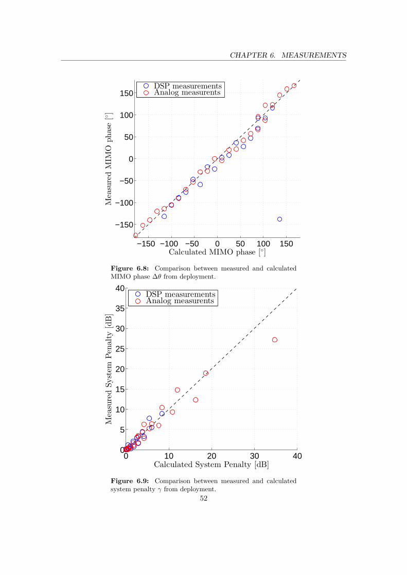
CHAPTER 6. MEASUREMENTS
−150 −100 −50 0 50 100 150
−150
−100
−50
0
50
100
150
Calculated MIMO phase [◦]
MeasuredMIM
Ophase[◦]
DSP measurementsAnalog measurents
Figure 6.8: Comparison between measured and calculatedMIMO phase ∆θ from deployment.
0 10 20 30 400
5
10
15
20
25
30
35
40
Calculated System Penalty [dB]
MeasuredSystem
Pen
alty
[dB]
DSP measurementsAnalog measurents
Figure 6.9: Comparison between measured and calculatedsystem penalty γ from deployment.
52
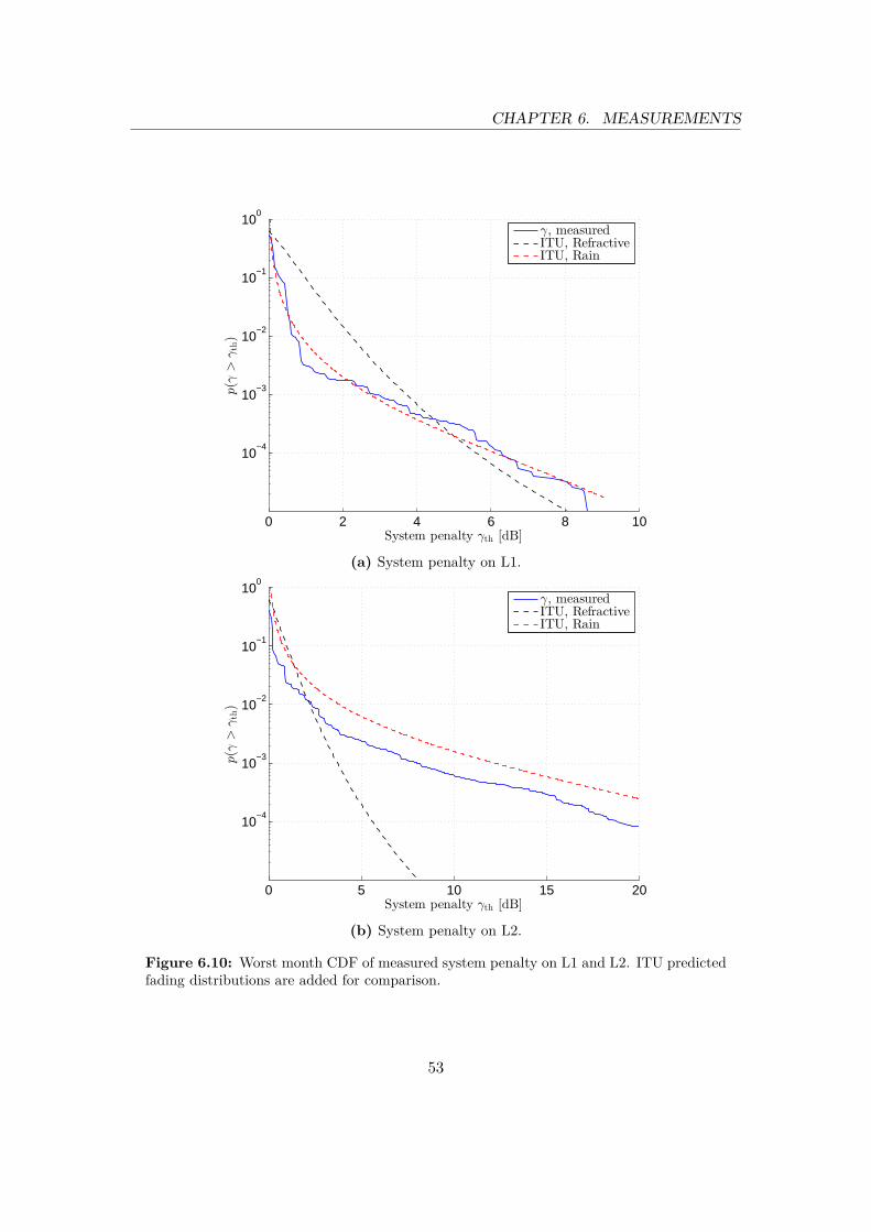
CHAPTER 6. MEASUREMENTS
0 2 4 6 8 10
10−4
10−3
10−2
10−1
100
System penalty γth [dB]
p(γ
>γth)
γ, measuredITU, RefractiveITU, Rain
(a) System penalty on L1.
0 5 10 15 20
10−4
10−3
10−2
10−1
100
System penalty γth [dB]
p(γ
>γth)
γ, measuredITU, RefractiveITU, Rain
(b) System penalty on L2.
Figure 6.10: Worst month CDF of measured system penalty on L1 and L2. ITU predictedfading distributions are added for comparison.
53

7Analysis
In this section, we present an analysis of the performance of a narrow-band systemgiven a Rician channel model (5.9). This analysis can help us to gain understandingof the performance of MIMO systems during refractive fading. In particular, we aremainly interested in the deep fading region with the multipath characteristic 10dB-per-decade slope of the fade depth. As availability is one of the key factors for microwavelinks and high power margins are usually employed, outages most typically occur in thisfading region [1]. The 10dB-per-decade slope characteristic is well-documented for real-world SISO links and therefore it is interesting to investigate if MIMO system penaltydistribution have similar properties, and if SISO and MIMO system penalties can berelated to each other.
We will present some numerical simulations to demonstrate the effect of multipath activ-ity and the significance of correlation of MIMO paths given Rician or Rayleigh channels.In particular, we consider a 2×2 ZF-MIMO and a 2×2 SVD-MIMO system with optimaldeployment (η = 1), thus HLOS from (5.9) will have full rank. Later we will investigatethe penalty distribution in terms of sub-optimal deployment.
7.1 Multipath Activity
In this section we present simulations of the impact of multipath activity (multipathfading). In this scope the multipath fading represent fading during abnormal refractiveconditions according to [2] and measurements in Section 6.3. In simulations we firstconsider a ZF-MIMO system in a Rician channel (5.9) for a changing value of the Ricianfactor κ. Generally in microwave links, multipath fading is often associated with reduc-tion of the overall received power of the signal, but to narrow down on the multipath
54
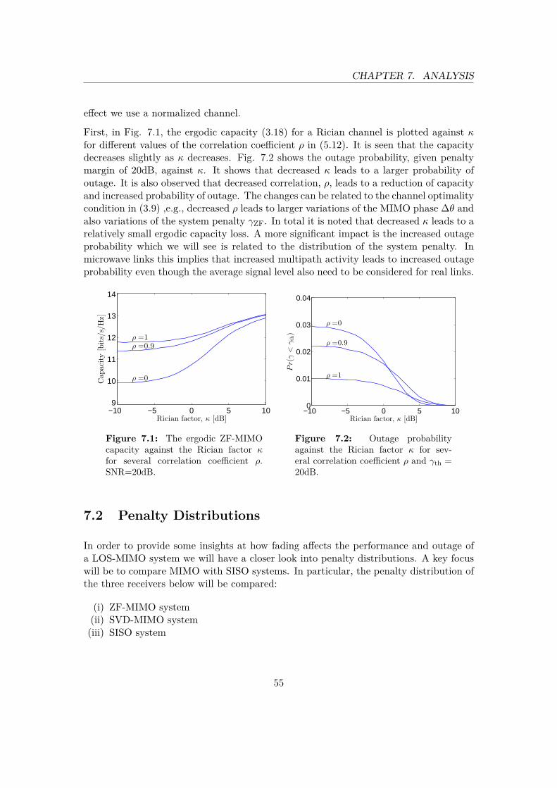
CHAPTER 7. ANALYSIS
effect we use a normalized channel.
First, in Fig. 7.1, the ergodic capacity (3.18) for a Rician channel is plotted against κfor different values of the correlation coefficient ρ in (5.12). It is seen that the capacitydecreases slightly as κ decreases. Fig. 7.2 shows the outage probability, given penaltymargin of 20dB, against κ. It shows that decreased κ leads to a larger probability ofoutage. It is also observed that decreased correlation, ρ, leads to a reduction of capacityand increased probability of outage. The changes can be related to the channel optimalitycondition in (3.9) ,e.g., decreased ρ leads to larger variations of the MIMO phase ∆θ andalso variations of the system penalty γZF. In total it is noted that decreased κ leads to arelatively small ergodic capacity loss. A more significant impact is the increased outageprobability which we will see is related to the distribution of the system penalty. Inmicrowave links this implies that increased multipath activity leads to increased outageprobability even though the average signal level also need to be considered for real links.
−10 −5 0 5 109
10
11
12
13
14
ρ =0
ρ =0.9ρ =1
Cap
acity[bits/s/Hz]
Rician factor, κ [dB]
Figure 7.1: The ergodic ZF-MIMOcapacity against the Rician factor κfor several correlation coefficient ρ.SNR=20dB.
−10 −5 0 5 100
0.01
0.02
0.03
0.04
ρ =0
ρ =0.9
ρ =1
Pr(γ
<γth)
Rician factor, κ [dB]
Figure 7.2: Outage probabilityagainst the Rician factor κ for sev-eral correlation coefficient ρ and γth =20dB.
7.2 Penalty Distributions
In order to provide some insights at how fading affects the performance and outage ofa LOS-MIMO system we will have a closer look into penalty distributions. A key focuswill be to compare MIMO with SISO systems. In particular, the penalty distribution ofthe three receivers below will be compared:
(i) ZF-MIMO system(ii) SVD-MIMO system(iii) SISO system
55

CHAPTER 7. ANALYSIS
The penalty for a SISO system γSISO is equivalent to a single path attenuation. Accord-ingly, if ρ = 1 the fading can be seen as a scalar factor wherefore all four systems willhave equal penalty distribution. We first look at the system penalty γ distribution inthe Rician channel with ρ = 1 for some values of κ in Fig. 7.3. It is seen that the tails ofthe distributions follow the 10dB-per-decade slope for various values of κ which suggeststhat Rician channels can model this 10dB-per-decade characteristic.
0 10 20 30 40
10−4
10−3
10−2
10−1
100
κ = 0
3
5
7
9
System penalty γth [dB]
Pr(γ
>γth)
Figure 7.3: System penalty CCDF for all systems in afully correlated Rician channel given ρ = 1 for some valuesof κ.
To gain insight into how the correlation coefficient ρ affects the penalty distributionswe conducted simulations in Fig. 7.4 and Fig. 7.5. In Fig. 7.4 we consider a correlatedRayleigh channel (5.10) as a typical worst case of multipath fading. In earlier studies theRayleigh channel has often been used to model severe refractive fading for microwavelinks [20, 22, 28].
The complementary cumulative distribution function (CCDF) of the penalty for the 2×2ZF-MIMO receiver in the Rayleigh channel is shown in Fig. 7.4a for various values of ρ.The distribution of γSISO is included for comparison and it remains equal to γZF givenρ = 1. Simulations show that the distribution γZF is moderately affected by ρ. The slopeof the distribution tails follows a 10dB-per-decade slope, equivalent to γSISO. Reducedpath correlation corresponds to an additional penalty. Next, the penalty distribution ofan SVD-MIMO receiver is plotted in Fig. 7.4b. It is seen that the SVD-MIMO receiverperforms similarly to or better than the SISO receiver in terms of outage. Especially, theimprovement becomes more significant as the correlation coefficient ρ decreases, whichcan be explained by reduced probability of large penalties.
56

CHAPTER 7. ANALYSIS
0 10 20 30 40
10−4
10−3
10−2
10−1
100
ρ = 1
00.90.99
System penalty γth [dB]
Pr(γ>
γth)
SISOZF-MIMO
(a) System penalty CCDF for ZF-MIMO system.
0 10 20 30 40
10−4
10−3
10−2
10−1
100
ρ = 1
0
0.9
0.99
System penalty γth [dB]
Pr(γ>
γth)
SISOSVD-MIMO
(b) System penalty CDF for SVD-MIMO system.
Figure 7.4: System penalty CCDF for ZF-MIMO and SVD-MIMO systems in correlatedRayleigh channel for several values of ρ.
In Fig. 7.5 we consider a Rician channel (5.9) with κ = 5 , which describes a channelwith a rich multipath environment and a significant LOS component. The CCDF of thepenalty for the 2 × 2 ZF-MIMO system is shown in Fig. 7.5a for various values of ρ.Similar to Rayleigh channel, simulations show that the distribution γZF is affected by ρ
57

CHAPTER 7. ANALYSIS
and the slope of the distribution tails follows the 10dB-per-decade slope. In differencewith the Rayleigh channel reduced path correlation can lead to both a penalty or a gaindepending on the degree of correlation. It is not in scope of this report to fully study thiseffect but it may be subjected to further studies. As seen in Fig. 7.5b for SVD-MIMOsystem, there is a reduced probability of large penalties over the SISO system. Theimprovement also increases for lower values of ρ.
A comparison of the two MIMO systems, the SISO system and an additional MISOsystem are shown in Fig. 7.6. The Multiple-Input-Single-Output (MISO) is added as areference as such systems are currently deployed in space diversity configurations [1, 2].The penalty γMISO is equivalent to the least attenuation signal at the receiver whichcorresponds to the selective combining solution [8]. An interesting observation for the2 × 2 MIMO system is that the distribution of γZF closely follows the distribution ofγSISO, and also the distribution of γSVD follows the distribution of γMISO. This is mostlikely due to the fact that the multipath fading can affect the channel orthogonalitycondition (3.9) and thus cause additional penalty.
For microwave links, the result of this section can be summarized as follows. For multi-path fading, the results shows that slightly changed probability of outage can be expectedfor ZF system. This change in outage probability can be related to a average penaltyoffset. However, for SVD systems a general improvement of the outage probability canbe expected.
58

CHAPTER 7. ANALYSIS
0 10 20 30 40
10−4
10−3
10−2
10−1
100
ρ = 10
0.90.99
System penalty γth [dB]
Pr(γ>
γth)
SISOZF-MIMO
(a) System penalty CCDF for ZF-MIMO system.
0 10 20 30 40
10−4
10−3
10−2
10−1
100
ρ = 1
0
0.90.99
System penalty γth [dB]
Pr(γ>
γth)
SISOSVD-MIMO
(b) System penalty CDF for SVD-MIMO system.
Figure 7.5: System penalty CCDF for ZF-MIMO and SVD-MIMO systems in correlatedRician channel for κ = 5 for several values of ρ.
59

CHAPTER 7. ANALYSIS
0 10 20 30 40
10−4
10−3
10−2
10−1
100
System penalty γth [dB]
Pr(γ
>γth)
SISOZF-MIMOMISOSVD-MIMO
(a) System penalty CCDF in Rayleigh channel given ρ = 0.9
0 10 20 30 40
10−4
10−3
10−2
10−1
100
System penalty γth [dB]
Pr(γ
>γth)
SISOZF-MIMOMISOSVD-MIMO
(b) System penalty CCDF in Rician channel given κ = 5 andρ = 0.9
Figure 7.6: A comparison of the system penalty for all system in the Rayleigh and Ricianchannel.
60

CHAPTER 7. ANALYSIS
7.3 Deployment Penalty in Fading Channels
This section is devoted to the study of consequences of sub-optimal deployment duringdeep fades. Recall the deployment conditions for determenistic channel HLOS, see (3.9)and (3.14). The Rayleigh and Rician distribution of (5.9) for κ = 5 is used to simulatethe deep fade region.
Simulations have shown that for a correlated Rayleigh and Rician channels sub-optimaldeployment (η < 1) translates to an average additional penalty. The deployment penaltyplotted against η for the Rayleigh channel is given in Fig. 7.7. It reveals an increasedpenalty as η decreases, similar as the deployment penalty of a deterministic channel. Itis noted that in an uncorrelated Rayleigh channel, ρ = 0, the system performance isindependent of the deployment and thus the system experiences no extra penalty due todeployment. In practise this means channels with less correlated fading, such as severerefractive fading in LOS microwave links or in typical access channels, allows for smallerantenna separation.
1 0.8 0.6 0.4 0.2 00
10
20
30
40
50
ρ =0.9
0.99
1
Dep
loymentpen
alty
[dB]
Deployment number, η
Figure 7.7: Additional ZF-MIMO deployment penalty in a Rayleigh channel against de-ployment number η for some correlation coefficients ρ.
It was shown in Fig. 3.3a in Chapter 3 that a deterministic LOS channel is subjectedto a deployment penalty if the deployment is sub-optimal (η < 1). Since the Ricianchannel includes a deterministic component the deployment predicted to be higher thanfor a pure Rayleigh channel which is shown in Fig. 7.8.
61

CHAPTER 7. ANALYSIS
1 0.8 0.6 0.4 0.2 00
10
20
30
40
50
ρ =0
0.9
0.99
1
Dep
loymentpen
alty[dB]
Deployment number, η
Figure 7.8: Additional ZF-MIMO deployment penalty in a Rician channel with κ = 5against deployment number η for some correlation coefficients ρ.
62

8Discussion
Channel models and performance prediction can be challenging to find for LOS mi-crowave links if they should be both accurate and general in terms of deployment, fre-quency and hop length. Several different approaches have been proposed such as theITU method or analytical models [2, 19]. All methods and models involve a trade-offbetween complexity, accuracy and how general they are.
For unobstructed links, two mechanisms have been found to affect the performance andcause outages, dominantly rain and refractivity related effects. As for most atmosphericeffects the occurrence and severity of these mechanisms depends on climate, terrain,hop-length and frequency. In earlier works, including the ITU model for SISO links,rain fading is modelled as attenuation of the received signal [2]. From real-world MIMOmeasurements we found that rain attenuation can be assumed to be completely correlatedbetween all MIMO paths. For rain fading under this assumption, all prediction methodsfor SISO links can directly be used for MIMO links.
Refractive fading on SISO links are usually modelled as multipath fading in combinationwith an additional frequency flat signal attenuation[2, 16, 22, 25]. Real-world measure-ments and prior studies show that the Rayleigh model and Rician model can also be usedto describe multipath fading event for LOS MIMO links. It is expected from mediumand long haul links that the fading may be frequency selective as well. A path corre-lation coefficient ρ is introduced to describe the correlation between the MIMO paths.It is reasonable that the correlation coefficient is a function of deployment, path length,frequency and fade depth. From measurements and studies on spatial diversity, theMIMO path correlation is expected to be high. This is a reasonable assumption sincethe spatial separation between MIMO paths are often small.
Simulations have shown that when calculating the outage probability for a MIMO link,uncorrelated fading among the MIMO paths can be statistically modelled as penalty/gain
63
CHAPTER 8. DISCUSSION
offset when compared with a SISO link. This is true for a ZF receiver structure, similaras the prototype receiver used in the test links. Such a penalty/gains can be handledwith an appropriate fade margin. For optimal system structure such as the SVD-MIMOsystem the probability of large system penalties are reduced, compared with a SISOsystem. This is likely due to the inherent diversity of the optimal systems. If the fadingis fully correlated, it will result in an equal system penalty for both MIMO and SISOsystems.
Given a frequency selective channel and an arbitrary receiver, it is difficult to accuratelypredict outage. In this case, the performance is dependent on the specific receiver.The method used for SISO systems is not easily applied to MIMO systems since theMIMO paths can have uncorrelated fading. In our long-term measurement, we didnot capture any frequency selective fading in the two prototype links. This may havebeen because the multipath delay of the trial was too small to result in any in-banddistortion. More measurements on longer frequency selective LOS-MIMO channel areneeded to fully understand the dispersive fading on MIMO link. It is worth mentioning,simulations performed by [9] reveals that current linear MIMO equalizers are able tohandle frequency selective fading but to a larger penalty than for a comparable SISOsystem. It is not in the scope of this report to derive a more general method to predictoutage and performance on dispersive LOS-MIMO links.
Roughly speaking, MIMO systems can be divided into two different user cases: shorthaul, high frequency links, and long haul, low frequency links where available spectrum islimited. In both cases MIMO technology offers an excellent method to increase spectrumefficiency and throughput. For frequencies above 15-20GHz rain is the dominant fading.Rain attenuation increases rapidly with frequency and hop length, which limits the hop-length and upper frequency for any practical link. Lower frequency links are usuallylimited by refractive fading.
Short haul MIMO links have already successfully been deployed by Ericsson Research andthe limiting rain fading is well understood from this report. It is likely that the increasedspectral efficiency offered by MIMO technology will make the technology attractive forlong-haul links in the future. While it should be possible to deploy a long haul MIMO linktoday, our understanding of the long haul MIMO channel is still limited and especiallythe impact of frequency selective fading. Moreover, a big drawback is also the largeantenna separation needed for the deployment. Even though long-haul links might beless common it is still valuable to be able to predict the performance and hence furtherinvestigation is needed. The ITU model can, verified by measurement from real-worldlinks and under the assumption of high correlation, most likely provide satisfactorypredictions for most short to medium-haul links (<20km).
64

9Conclusions
In this report we have studied prior work and performed real world measurements onLOS-MIMO microwave links to provide insights in fading characteristics and perfor-mance over LOS-MIMO microwave channels. From the work we have come to thefollowing conclusions.
• We introduce a practical MIMO phase metric, ∆θ (3.15) simply referred as MIMOphase and define an optimality criterion for 2× 2 LOS-MIMO systems (3.17) thatis equivalent to that in [5, 7].
• System penalty γ is defined in (3.22) and (3.25) as an equivalent to fade attenuationof a SISO system. Penalty is important for MIMO systems since not only thereceived power but also the structure of the MIMO channel affects performance.
• Motivated by measurements subjected to rain fading, rain is modelled as scalarattenuation of the nominal signal level for LOS-MIMO links. This results in anequivalent system penalty for both MIMO and SISO systems. Current rain fadingprediction methods, such as those from ITU, can straightforwardly be applied onLOS-MIMO links.
• Predicted by the ITU method, the occurrence and severity and refractive fadingincrease with both geoclimatic factors, hop length and frequency. The methodpredict a 10dB-per-decade slope of deep fade probabilities for SISO systems as inFig. 5.1
• Motivated by measurements subjected to short term refractive fading characteris-tics, a correlated Rician channel model (5.9) has been proposed.
• It is shown by simulations that in the deep fading region, the distribution of thepenalty γZF follows γSISO with a 10dB-per-decade slope, given the assumption of
65

CHAPTER 9. CONCLUSIONS
Rayleigh/Rician channels.
• Reduced correlation leads to a penalty offset from the SISO system to the ZF-MIMO system when calculating outage probability.
• For a SVD-MIMO system a general improvement of outage probabilities can beexpected to outperform a SISO system. The improvement increases for decreasedρ.
• Sub-optimal antenna deployment causes an additional system penalty as in Fig. 3.3a.In Rayleigh/Rician fading channels the average additional penalty during deepfades is related to the correlation of the MIMO paths. Reduced correlation leadsto smaller average additional deployment penalty.
9.1 Further Studies
Exhaustive studies are still required to fully understand fading mechanisms in microwaveLOS-MIMO channels. Especially, fading correlation and frequency selective fading arenot fully investigated. More measurements and experiments on real links needs to beperformed to capture these effects. Given limited measurements, simulations have beenperformed but more can be done also in this area. We have seen from simulations thatthe choice of system structure can have large impact on the performance in the deepfading region.
One of the key goals of this work was to investigate performance over LOS-MIMOchannels and if possible, suggest relevant modifications of the existing standards, suchas ITU models. To further increase the understanding of the topics, we will highlightsome areas that can be investigated in more details.
• The study of correlated fading in Rayleigh/Rician channels, and its impact onsystem performance and outage probabilities will be useful.
• More studies are required on correlation and frequency selectivity in LOS-MIMOchannels in terms of distance, deployment, frequency etc. Measurements fromreal-world links are useful to characterize these effects and enrich the propagationmodels.
• Based on increased knowledge of the channel, studies on efficient receiver struc-tures, in terms of complexity and performance, in correlated frequency selectiveMIMO channels are useful.
66

Bibliography
[1] A. Käse, Radio Path Planning Handbook, Ericsson GmbH, 2006.
[2] International Telecommunication Union, ITU-R Recommendation P.530-14, Propa-gation data and prediction methods required for the designof terrestrial line-of-sightsystems (2012).
[3] T. Manning, Microwave radio transmission design guide, Artech House, 2009.
[4] F. Bohagen, P. Orten, G. Oien, Modeling and analysis of a 40 ghz mimo system forfixed wireless access, in: Vehicular Technology Conference, 2005. VTC 2005-Spring.2005 IEEE 61st, Vol. 3, 2005, pp. 1691–1695 Vol. 3.
[5] D. Gesbert, H. Bolcskei, D. A. Gore, A. J. Paulraj, Outdoor mimo wireless channels:Models and performance prediction, IEEE Transactions on Communications 50 (12)(2002) 1926–1934.
[6] D. Tse, Fundamentals of wireless communication, Cambridge university press, 2005.
[7] F. Bohagen, P. Orten, G. E. Oien, Design of optimal high-rank line-of-sight mimochannels, Wireless Communications, IEEE Transactions on 6 (4) (2007) 1420–1425.
[8] A. Goldsmith, Wireless communications, Cambridge university press, 2005.
[9] T. Ingason, H. Liu, Line-of-sight mimo for microwave links-adaptive dual polarizedand spatially separated systems, Master’s thesis, Chalmers University of Technology(2009).
[10] International Telecommunication Union, ITU-R Recommendation P.838-3,Specificattenuation model for rain for use in prediction methods (2005).
[11] H. Xu, T. S. Rappaport, R. J. Boyle, J. H. Schaffner, Measurements and models for38-ghz point-to-multipoint radiowave propagation, IEEE Journal on Selected Areasin Communications 18 (3) (2000) 310–321.
67
BIBLIOGRAPHY
[12] International Telecommunication Union, ITU-R Recommendation P.453-10, Theradio refractive index: its formula and refractivity data (2012).
[13] B. Bean, E. Dutton, Radio meteorology. national bureau of standards monogr(1968).
[14] M. Grabner, V. Kvicera, Atmospheric refraction and propagation in lower tropo-sphere, Electromagnetic Waves (2011) 139–156.
[15] I. Sirkova, M. Mikhalev, Influence of tropospheric duct parameters changes on mi-crowave path loss, in: Proceedings of the XXXVIII International Scientific Confer-ence on Information, Communication & Energy Systems & Technologies, ICEST,2003, pp. 16–18.
[16] M. Shafi, Statistical analysis/simulation of a three ray model for multipath fadingwith applications to outage prediction, IEEE Journal on Selected Areas in Commu-nications 5 (3) (1987) 389–401.
[17] E. Costa, The effects of ground-reflected rays and atmospheric inhomogeneities onmultipath fading, IEEE Transactions on Antennas and Propagation 39 (6) (1991)740–745.
[18] M. Thompson Jr, H. Janes, Measurements of phase stability over a low-level tropo-spheric path, J. Research Natl. Bur. Standards D 63 (1959) 45.
[19] P. Almers, E. Bonek, A. Burr, N. Czink, M. Debbah, V. Degli-Esposti, H. Hofstetter,P. Kyö, D. Laurenson, G. Matz, et al., Survey of channel and radio propagationmodels for wireless mimo systems, EURASIP Journal on Wireless Communicationsand Networking 2007.
[20] A. Vigants, Space-diversity performance as a function of antenna separation, IEEETransactions on Communication Technology 16 (6) (1968) 831–836.
[21] T. Lee, S. Lin, A model of space diversity for microwave radio against thermal noisecaused outage during multipath fading, in: IEEE Global Telecommunications Con-ference, 1988, and Exhibition.’Communications for the Information Age.’ConferenceRecord, GLOBECOM’88., IEEE, 1988, pp. 1440–1446.
[22] K. Pearson, Method for the prediction of the fading performance of a multisectionmicrowave link, Proceedings of the Institution of Electrical Engineers 112 (7) (1965)1291–1300.
[23] W. Barnett, Multipath propagation at 4, 6, and 11 ghz, Bell System TechnicalJournal 51 (2) (1972) 321–361.
[24] R. G. McKay, M. Shafi, Multipath propagation measurements on an overwater pathin new zealand, IEEE Transactions on Communications 36 (7) (1988) 781–788.
68

BIBLIOGRAPHY
[25] W. Rummler, A new selective fading model: Application to propagation data, Bellsystem technical journal 58 (5) (1979) 1037–1071.
[26] F. Bøhagen, Modeling, characterization and design of line-of-sight wireless mimochannels, Ph.D. thesis, University of Oslo (2007).
[27] Experimental results on phase measurement of 2× 2 microwave line-of-sight mimolinks, Ericsson Internal Report.
[28] S.-F. Ong, C.-F. Hu, Propagation measurements on an over-water, line-of-sightlink in singapore, in: Proceedings of 1997 International Conference on Information,Communications and Signal Processing, 1997. ICICS., Vol. 3, 1997, pp. 1714–1718vol.3.
69