measurement of the production cross section of heavy quark...
TRANSCRIPT

Physik-Department
Measurement of the production cross section of
heavy quark jets in association with a W boson
with the ATLAS detector at the LHC
Dissertation
von
Marco Vanadia
Munchen
Juni 2013


TECHNISCHE UNIVERSITAT MUNCHEN
Max-Planck-Institut fur Physik(Werner-Heisenberg-Institut)
Lehrstuhl fur Experimentalphysik
Measurement of the production cross section ofheavy quark jets in association with a W boson
with the ATLAS detector at the LHC
Marco Vanadia
Vollstandiger Abdruck der von der Fakultat fur Physik der Technischen Universitat Munchen
zur Erlangung des akademischen Grades eines
Doktors der Naturwissenschaften (Dr. rer. nat.)
genehmigten Dissertation.
Vorsitzender: Univ-Prof. Dr. M. Beneke
Prufer der Dissertation:
1. Priv.-Doz. Dr. H. Kroha
2. Univ-Prof. Dr. L. Oberauer
Die Dissertation wurde am 05.06.2013 bei der Technischen Universitat Munchen einge-
reicht und durch die Fakultat fur Physik am 12.06.2013 angenommen.


Abstract
In this thesis the production of a W boson in association with heavy-quark jets has been
studied in proton-proton collisions at a centre-of-mass energy of 7 TeV with the ATLAS
detector at the Large Hadron Collider (LHC).
For the identification of the W bosons and of the heavy quarks their semileptonic decays
have been used. For this purpose, detailed studies of the muon reconstruction efficiencies
of the ATLAS detector have been performed.
The associated production of a W boson with bottom quark jets represents an important
background for searches for the Higgs boson and beyond Standard Model physics. It
is therefore important to verify experimentally the Standard Model predictions for this
process in the new energy regime of the LHC. The cross sections for W boson production
together with a b-jet and zero or one additional jet have been measured for the first time at
LHC energies and were found to be consistent with next-to-leading order QCD predictions.
The W boson production in association with a charm quark jet is of particular interest
because of the sensitivity to the strange quark content of the proton which is still rather
poorly constrained by experiments. The cross section measurements for this process in this
thesis are an important input for the determination of the strange quark parton density
function in the energy regime of the LHC.


Contents
Introduction 1
1 The Standard Model of Strong and Electroweak Interactions 3
1.1 Electroweak interactions . . . . . . . . . . . . . . . . . . . . . . . . . . . . . 4
1.2 The Higgs mechanism . . . . . . . . . . . . . . . . . . . . . . . . . . . . . . 6
1.3 Quantum chromodynamics . . . . . . . . . . . . . . . . . . . . . . . . . . . 7
1.4 Physics beyond the Standard Model . . . . . . . . . . . . . . . . . . . . . . 7
2 W and Z boson production at the LHC 9
2.1 Theoretical description of pp collisions . . . . . . . . . . . . . . . . . . . . . 9
2.2 Overview of W± and Z boson production at colliders . . . . . . . . . . . . . 11
2.3 Monte Carlo generators . . . . . . . . . . . . . . . . . . . . . . . . . . . . . 13
3 The ATLAS experiment at the Large Hadron Collider 15
3.1 The Large Hadron Collider . . . . . . . . . . . . . . . . . . . . . . . . . . . 15
3.2 The ATLAS detector . . . . . . . . . . . . . . . . . . . . . . . . . . . . . . . 17
3.2.1 Notation and conventions . . . . . . . . . . . . . . . . . . . . . . . . 19
3.2.2 The Magnet System . . . . . . . . . . . . . . . . . . . . . . . . . . . 19
3.2.3 The Inner Detector . . . . . . . . . . . . . . . . . . . . . . . . . . . . 20
3.2.3.1 The Pixel Detector . . . . . . . . . . . . . . . . . . . . . . 21
3.2.3.2 The Semiconductor Tracker . . . . . . . . . . . . . . . . . . 21
3.2.3.3 The Transition Radiation Tracker . . . . . . . . . . . . . . 21
3.2.4 The Calorimeter System . . . . . . . . . . . . . . . . . . . . . . . . . 21
3.2.4.1 The Electromagnetic Calorimeter . . . . . . . . . . . . . . 22
3.2.4.2 The Hadron Calorimeter . . . . . . . . . . . . . . . . . . . 23
3.2.5 The Muon Spectrometer . . . . . . . . . . . . . . . . . . . . . . . . . 23
3.2.5.1 Monitored Drift Tube chambers . . . . . . . . . . . . . . . 25
3.2.5.2 Cathode Strip Chambers . . . . . . . . . . . . . . . . . . . 27
3.2.5.3 Alignment system for the precision chambers . . . . . . . . 28
3.2.5.4 Resistive Plate Chambers . . . . . . . . . . . . . . . . . . . 28
3.2.5.5 Thin Gap Chambers . . . . . . . . . . . . . . . . . . . . . . 28
3.2.6 The Trigger System . . . . . . . . . . . . . . . . . . . . . . . . . . . 29
iii

iv Contents
3.2.6.1 The first-level muon trigger system . . . . . . . . . . . . . 29
3.2.7 Luminosity measurement in the ATLAS experiment . . . . . . . . . 30
4 Reconstruction of physics objects 31
4.1 Detector simulation . . . . . . . . . . . . . . . . . . . . . . . . . . . . . . . . 31
4.2 Charged particle and vertex reconstruction in the Inner Detector . . . . . . 32
4.3 Electrons and Photons . . . . . . . . . . . . . . . . . . . . . . . . . . . . . . 33
4.3.1 Electron reconstruction . . . . . . . . . . . . . . . . . . . . . . . . . 33
4.3.2 Photon reconstruction . . . . . . . . . . . . . . . . . . . . . . . . . . 34
4.4 Jets . . . . . . . . . . . . . . . . . . . . . . . . . . . . . . . . . . . . . . . . 35
4.4.1 Jet Reconstruction . . . . . . . . . . . . . . . . . . . . . . . . . . . . 35
4.4.2 Jet quality . . . . . . . . . . . . . . . . . . . . . . . . . . . . . . . . 36
4.4.3 Jet energy measurement . . . . . . . . . . . . . . . . . . . . . . . . . 36
4.4.4 Heavy flavour jet tagging . . . . . . . . . . . . . . . . . . . . . . . . 37
4.4.4.1 The SV0 b-tagging algorithm . . . . . . . . . . . . . . . . . 38
4.5 τ leptons . . . . . . . . . . . . . . . . . . . . . . . . . . . . . . . . . . . . . 39
4.6 Transverse missing energy . . . . . . . . . . . . . . . . . . . . . . . . . . . . 39
4.7 Muons . . . . . . . . . . . . . . . . . . . . . . . . . . . . . . . . . . . . . . . 39
4.8 Track and calorimeter isolation . . . . . . . . . . . . . . . . . . . . . . . . . 42
5 Muon reconstruction performance 43
5.1 Measurement of the muon reconstruction efficiency . . . . . . . . . . . . . . 43
5.1.1 Dependence on the Muon Spectrometer regions . . . . . . . . . . . . 43
5.1.2 The Tag-and-Probe method . . . . . . . . . . . . . . . . . . . . . . . 44
5.1.3 Data and Monte Carlo samples . . . . . . . . . . . . . . . . . . . . . 45
5.1.4 Event selection . . . . . . . . . . . . . . . . . . . . . . . . . . . . . . 47
5.1.4.1 ID track quality cuts . . . . . . . . . . . . . . . . . . . . . 47
5.1.4.2 Tag muon selection . . . . . . . . . . . . . . . . . . . . . . 48
5.1.4.3 Probe muon selection . . . . . . . . . . . . . . . . . . . . . 48
5.1.4.4 Matching . . . . . . . . . . . . . . . . . . . . . . . . . . . . 51
5.1.5 Inner Detector reconstruction efficiency . . . . . . . . . . . . . . . . 51
5.1.6 Muon reconstruction efficiency . . . . . . . . . . . . . . . . . . . . . 55
5.1.7 Systematic errors of the muon efficiency scale factors . . . . . . . . . 57
5.1.8 Muon reconstruction efficiency for low-pT muons . . . . . . . . . . . 59
5.2 Measurement of the muon trigger and isolation efficiency . . . . . . . . . . . 60
5.3 Heavy flavour jet tagging efficiency . . . . . . . . . . . . . . . . . . . . . . . 62
5.4 Conclusion . . . . . . . . . . . . . . . . . . . . . . . . . . . . . . . . . . . . 68
6 Measurement of the W+ b-jet production cross section 69
6.1 Data samples used for the analysis . . . . . . . . . . . . . . . . . . . . . . . 69
6.1.1 Overlap removal for the Alpgen W+ jets samples . . . . . . . . . . 70
6.2 Event selection . . . . . . . . . . . . . . . . . . . . . . . . . . . . . . . . . . 72

Contents v
6.2.1 Preselection . . . . . . . . . . . . . . . . . . . . . . . . . . . . . . . . 72
6.2.2 Trigger requirements . . . . . . . . . . . . . . . . . . . . . . . . . . . 72
6.2.3 Lepton selection . . . . . . . . . . . . . . . . . . . . . . . . . . . . . 73
6.2.4 W boson selection . . . . . . . . . . . . . . . . . . . . . . . . . . . . 74
6.2.5 Jet selection and b-jet tagging . . . . . . . . . . . . . . . . . . . . . . 75
6.3 Background estimation . . . . . . . . . . . . . . . . . . . . . . . . . . . . . . 75
6.3.1 The W+ jets background . . . . . . . . . . . . . . . . . . . . . . . . 75
6.3.2 The tt background . . . . . . . . . . . . . . . . . . . . . . . . . . . . 76
6.3.3 The QCD multi-jet background . . . . . . . . . . . . . . . . . . . . . 78
6.3.3.1 Electron channel . . . . . . . . . . . . . . . . . . . . . . . . 78
6.3.3.2 Muon channel . . . . . . . . . . . . . . . . . . . . . . . . . 78
6.3.3.3 QCD multi-jet mSV templates . . . . . . . . . . . . . . . . 80
6.4 Cross section determination . . . . . . . . . . . . . . . . . . . . . . . . . . . 80
6.5 Systematic uncertainties . . . . . . . . . . . . . . . . . . . . . . . . . . . . . 83
6.6 Results of the fiducial cross section measurement . . . . . . . . . . . . . . . 85
7 Measurement of the W+ c-jet production cross section 89
7.1 Motivation . . . . . . . . . . . . . . . . . . . . . . . . . . . . . . . . . . . . 89
7.2 Measurement strategy . . . . . . . . . . . . . . . . . . . . . . . . . . . . . . 91
7.3 Samples used for the analysis . . . . . . . . . . . . . . . . . . . . . . . . . . 94
7.4 Event selection . . . . . . . . . . . . . . . . . . . . . . . . . . . . . . . . . . 95
7.4.1 Preselection . . . . . . . . . . . . . . . . . . . . . . . . . . . . . . . . 95
7.4.2 Trigger requirements . . . . . . . . . . . . . . . . . . . . . . . . . . . 95
7.4.3 Lepton selection . . . . . . . . . . . . . . . . . . . . . . . . . . . . . 96
7.4.3.1 Electron channel . . . . . . . . . . . . . . . . . . . . . . . . 96
7.4.3.2 Muon channel . . . . . . . . . . . . . . . . . . . . . . . . . 96
7.4.3.3 Lepton-jet overlap removal . . . . . . . . . . . . . . . . . . 97
7.4.3.4 Lepton efficiency corrections . . . . . . . . . . . . . . . . . 97
7.4.4 W boson selection . . . . . . . . . . . . . . . . . . . . . . . . . . . . 97
7.4.5 Jet selection . . . . . . . . . . . . . . . . . . . . . . . . . . . . . . . . 97
7.4.6 c-jet selection . . . . . . . . . . . . . . . . . . . . . . . . . . . . . . . 98
7.5 Background estimation . . . . . . . . . . . . . . . . . . . . . . . . . . . . . . 99
7.5.1 QCD multi-jet background . . . . . . . . . . . . . . . . . . . . . . . 99
7.5.1.1 Electron channel . . . . . . . . . . . . . . . . . . . . . . . . 100
7.5.1.2 Muon channel . . . . . . . . . . . . . . . . . . . . . . . . . 101
7.5.2 W+ light-jets background . . . . . . . . . . . . . . . . . . . . . . . . 104
7.5.2.1 Electron channel . . . . . . . . . . . . . . . . . . . . . . . . 104
7.5.2.2 Muon channel . . . . . . . . . . . . . . . . . . . . . . . . . 105
7.5.3 Refinement of the QCD multi-jet and W+ light-jets background
determination in the electron channel . . . . . . . . . . . . . . . . . 106
7.5.4 Z+ jets background . . . . . . . . . . . . . . . . . . . . . . . . . . . 107
7.6 Signal and background yields . . . . . . . . . . . . . . . . . . . . . . . . . . 109

vi Contents
7.7 W++ c-jet and W−+ c-jet production . . . . . . . . . . . . . . . . . . . . . 115
7.8 Yields as a function of the |η`| of the lepton from the W decay . . . . . . . 116
7.9 Cross section determination . . . . . . . . . . . . . . . . . . . . . . . . . . . 118
7.9.1 Determination of the selection efficiency . . . . . . . . . . . . . . . . 119
7.9.2 Determination of the extrapolation factor . . . . . . . . . . . . . . . 120
7.9.3 c-hadron fragmentation and decay . . . . . . . . . . . . . . . . . . . 120
7.10 Measurement of the W++ c-jet and W−+ c-jet production cross sections . 123
7.11 Systematic uncertainties . . . . . . . . . . . . . . . . . . . . . . . . . . . . . 124
7.11.1 Background estimation . . . . . . . . . . . . . . . . . . . . . . . . . . 124
7.11.2 Detector effects . . . . . . . . . . . . . . . . . . . . . . . . . . . . . . 126
7.11.3 Uncertainties in W + c signal modelling . . . . . . . . . . . . . . . . 128
7.12 W+ c-jet fiducial cross section results . . . . . . . . . . . . . . . . . . . . . 129
7.13 Combination of the electron and muon channels . . . . . . . . . . . . . . . . 131
7.14 Comparison with theoretical predictions . . . . . . . . . . . . . . . . . . . . 133
Conclusions 141
A Rejection of non-prompt muons 145
B Muon reconstruction performance in 2012 data 147
Bibliography 162
Acknowledgements 163

Nothing is insoluble. Nothing is hopeless.
Not while there’s life.
(Alan Moore, Watchmen)


Introduction
The Large Hadron Collider (LHC) at CERN is currently the largest particle accelerator
in the world. Located near Geneva, in a 27.5 km long underground tunnel, after nearly
two decades of planning and construction it started colliding protons steadily at a centre-
of-mass energy of√
s=7 TeV since March 2010, an energy never reached before at particle
colliders. In 2012 the centre-of-mass energy was raised to√
s=8 TeV. In early 2013 the
LHC went into shutdown for upgrades to increase beam energy and instantaneous lumi-
nosity. The LHC is the culmination of the physics experiments which tested and confirmed
the Standard Model of particle physics in this and the last century shaping our knowledge
of the most fundamental constituents of matters in the Universe.
The Standard Model is a theory of the electroweak and strong interactions between ele-
mentary particles which has been developed to its present form in the 1960s and 70s, with
quarks and leptons as fundamental constituents of matter and local gauge boson fields as
mediator of the interactions. The Standard Model successfully describes the experimen-
tal results obtained up to now and foreshadowed the existence of new phenomena and
particles which were observed in the years following its formulation, as the the neutral
weak current discovered with the Gargamelle bubble chamber at the CERN Proton Syn-
chrotron and the W and Z bosons discovered by the UA1 and UA2 experiments at the
CERN Super Proton Synchrotron. Many other experimental results in the last decades
strengthened the Standard Model description and shaped our current knowledge of the
fundamental constituents of matter with the discovery of new elementary particles: the
charm quark (at the Stanford Linear Accelerator Center and at the Brookhaven National
Laboratory), the bottom quark (by the E288 experiment at Fermilab), the τ lepton (at the
Stanford Linear Accelerator Center), the gluons (at DESY laboratories), the top quark
(by the CDF and D0 experiments at the proton-antiproton collider Tevatron at Fermilab)
and the τ neutrino (by the DONUT experiment at the Tevatron).
The measurements performed by the experiments at the Tevatron and at the CERN Large
Electron Positron (LEP) collider provided tests of the Standard Model with unprecedented
precision. The last missing piece of the Standard Model was one of its cornerstones: the
spinless Higgs boson which is related to the mechanism providing masses to the elementary
particles without violating local gauge invariance. The search for this particle lasted for
decades as the Standard Model makes no precise prediction for its mass.
1

2 Contents
Finally, on July 4th 2012, the ATLAS and the CMS experiments at the LHC announced
the discovery of a new particle with a mass of about 125 GeV/c2 and the characteristics
of the Higgs boson.
The experiments at the LHC test also other predictions of the Standard Model with high
precision and at the highest energies reached by accelerators so far.
ATLAS is a general-purpose detector designed to study proton-proton interactions at the
LHC with a very wide research program including Higgs boson searches, precision mea-
surements of the strong and electroweak interactions, top quark physics, flavour physics,
and searches for new physics beyond the Standard Model. In this thesis the cross sections
for the production of a W boson in association with heavy charm and bottom quark jets
predicted by the Standard Model has been measured with data collected by the ATLAS
experiment in 2010 and 2011. These measurements probe the perturbative calculations
and Monte Carlo descriptions of such processes, which are particularly relevant because
these productions represent important background for many Standard Model and beyond
Standard Model studies. Furthermore, the study of charm jets produced together with W
bosons provide important information on the strange quark content of the proton which
is currently known with high uncertainties.
In Chapter 1 a brief introduction to the Standard Model is given. Chapter 2 gives an
overview of the phenomenology of weak boson production at the LHC with particular fo-
cus on W+ jets production. In Chapter 3 the LHC and the ATLAS detector are described,
while in Chapter 4 an overview of the algorithms used for the evaluation of the trajectories
and the energies of particles, hadron jets and other observables is given. Chapter 5 presents
a detailed study of the performance of the ATLAS muon spectrometer and of the muon
identification in data, which are important for the measurements presented in this thesis
and for many other measurements by the ATLAS experiment involving muons. Chapter 6
describes the cross section measurement for the associated production of a W boson to-
gether with at least one bottom quark jet using data collected in 2010 [1]. In Chapter 7 the
cross section measurement using data collected in 2011 for the production of a W boson
in association with a charm quark jet is explained [2]. Both cross section measurements
have been produced by small analysis teams and are described in the respective chapters
with particular focus on the major contribution of this work.
Conventions
Throughout the thesis, the International System of Units [3, 4] is used. The speed of light,
however, is fixed to c = 1. Thus, masses, momenta and energies are expressed in the same
units, namely the eV = 1.602176565(35) ·10−19 J. Charges are expressed in units of the
electron charge.

Chapter 1
The Standard Model of Strong
and Electroweak Interactions
The Standard Model [5, 6, 7, 8] is our present best theory of the fundamental interactions
intercurring between elementary particles. It is extremely successful in describing the
experimental results of particle physics with high precision. Three of the four known
interactions are described by the Standard Model (see Table 1.1):
the strong interaction responsible for the binding of quarks in hadrons and of the
nucleons in nuclei,
the weak interaction responsible for instance for the radioactive β− decays,
and the electromagnetic interaction, responsible for the interactions between charged
particles.
The Standard Model is a relativistic quantum field theory invariant under the local gauge
transformation group
SU(3)C ⊗ SU(2)L ⊗ U(1)Y (1.1)
with the SU(3)C symmetry group of the strong interaction and the SU(2)L ⊗ U(1)Ygroup describing the electroweak interactions. The Standard Model comprises 12 elemen-
tary fermions, the gauge bosons of the SU(3)C ⊗ SU(2)L ⊗U(1)Y interactions between
the fermions and the Higgs boson responsible for the SU(2)L⊗U(1)Y symmetry breaking
which provides mass terms for the weak gauge bosons. These components are summarized
in Table 1.2. All particles have a corresponding anti-particle with opposite charge and the
same mass as a consequence of CPT invariance [9, 10, 11, 12].
The Standard Model particles are described by the following quantum fields:
Spinor fields Ψ for the fermions.
3

4 Chapter 1. The Standard Model of Strong and Electroweak Interactions
Vector gauge fields Ga, B, W i for the gluons and the electroweak bosons.
The Scalar Higgs boson field Φ.
The brief review of the Standard Model presented in this chapter is based on [13, 14, 15].
Table 1.1: Fundamental interactions
Interaction Range [m] Mediators Relative strength
Strong 10−15 gluons 1Weak 10−18 W± and Z0 bosons 10−13
Electromagnetic ∞ photon 10−2
Gravitational ∞ graviton (not discovered yet) 10−38
Table 1.2: Elementary particles in the Standard Model
Fermions (spin 1/2) Bosons (spin 1) Boson (spin 0)
Quarksu c b W±
Higgs bosond s t Z0
Leptonsνe νµ ντ γ0
e µ τ gluons
1.1 Electroweak interactions
In the Standard Model, the electroweak interaction is described by the symmetry group
SU(2)L ⊗ U(1)Y . (1.2)
As introduced first by Glashow in 1961 [5], three conserved weak currents are related to
the generators of the weak isospin group SU(2)L and one to the weak hypercharge group
U(1)Y . The observed charged weak currents can be identified as a combination of two
SU(2)L currents, while the neutral weak and the electromagnetic currents are derived
from a mixing of the SU(2) and U(1) currents.
The weak hypercharge Y is related to the electric charge Q and the third component of
the weak isospin I by:
Y = 2(Q− I3) . (1.3)
The elementary fermions included in the Standard Model are arranged in weak isospin
multiplets (see Table 1.3). The weak gauge bosons fields generated by the SU(2)L sym-
metry group couple only with left-handed fermions, which are included in isospin doublets.
Right-handed leptons and quarks represent isospin singlets. Right-handed neutrinos would
be non-interacting particles and are therefore not included in the Standard Model.

1.1. Electroweak interactions 5
Table 1.3: Quantum numbers of the elementary fermions in the Standard Model. The subscriptL indicates left-handed particles, the subscript R indicates right-handed particles.
Fermions I I3 Y Q
quarks
(ud
)L
(cs
)L
(tb
)L
1/2 1/2 1/3 2/3
1/2 -1/2 1/3 -1/3
uR cR tR 0 0 4/3 2/3
dR sR bR 0 0 -2/3 -1/3
leptons
(νee−
)L
(νµµ−
)L
(νττ−
)L
1/2 1/2 -1/2 01/2 -1/2 -1/2 -1
e−R µ−R τ−R 0 0 -2 -1
The physical electroweak bosons fields W±, Z0, A are linear combinations of the fields
corresponding to the generators of SU(2) and U(1), respectively the isospin triplet Wµ
and the hypercharge singlet Bµ.
W±,µ =1√2
(Wµ1 ∓ iW
µ2 ), (1.4)
are the mediators of the charged weak interaction,
Aµ = Bµcos(θW ) +Wµ3 sin(θW ), (1.5)
is the photon field and
Zµ = −Bµsin(θW ) +Wµ3 cos(θW ) (1.6)
the mediator of the neutral weak interaction. θW is the Weinberg mixing angle [16].
This model describes the left-handed charged weak currents and the neutral weak and elec-
tromagnetic currents interacting both with right-handed and left-handed fermions. The
four gauge bosons are massless according to the local gauge symmetry of the interactions.
However, the W and Z bosons have experimentally observed masses needed to explain the
short range of the weak interactions. Explicit mass terms introduced into the Standard
Model Lagrangian would break the gauge invariance and thus the renormalizability of the
field theory.

6 Chapter 1. The Standard Model of Strong and Electroweak Interactions
1.2 The Higgs mechanism
The solution for this problem is provided by the Higgs mechanism [17, 18, 19, 20, 21, 22]
introduced into the Standard Model by Weinberg [6] and Salam [7] at the end of the 1960s.
The Higgs mechanism employs spontaneous symmetry breaking by introducing gauge bo-
son masses. The Goldstone theorem [23, 24] states that the spontaneous breaking of a
global continuous symmetry generates massless Goldstone bosons. The Higgs mechanism
involves the spontaneous symmetry breaking of a local gauge symmetry, the SU(2)L ⊗ U(1)Ysymmetry of the electroweak interaction.
A new contribution has to be included into the Lagrangian of the Standard Model:
L = (Dµφ)†(Dµφ)− µ2φ†φ− λ(φ†φ)2 = (Dµφ)†(Dµφ)− V (φ) (1.7)
with Dµ = ∂µ + igI ·Wµ + ig′
2 Y Bµ and g, g′ being constants. This term describes
the propagation and interaction field of a complex scalar weak isospin doublet field with
Y = 1. Choosing a potential V (φ) with µ2 < 0 and λ > 0 the ground state is not
uniquely defined at |φ| = 0, but any state fulfilling the requirement
φ†φ =−µ2
2λ≡ v2
2. (1.8)
All ground states are connected by gauge transformations. An arbitrary ground state may
be chosen, for instance φ0 = 1√2
(0v
). The scalar Higgs field H(x) is a massive excitation
from this ground state,
φ(x) =1√2
( 0v+H(x)
), (1.9)
corresponding to a new neutral particle with mass mH =√−2µ2. Massless excitations in
the form of Goldstone bosons have been eliminated by gauge transformation into longitu-
dinal polarization states of the W and Z0 bosons. Inserting Eq. 1.9 into the Lagrangian
of Eq. 1.7 the following expression is obtained:
L =1
2(∂µH)2 − µ2H2 +
g2v2
4W+µ W
−µ +v2(g2 + g′2)
8ZµZ
µ
+ boson kinetic energy terms + higher order terms .
(1.10)
The spontaneously generated mass terms for the W± and Z bosons do not violate gauge
invariance and the photon remains massless. Mass terms for the fermions are also forbidden
by the global SU(2)L symmetry but can be generated preserving the gauge invariance by
introducing a new weak interaction between the fermions and the Higgs field.

1.3. Quantum chromodynamics 7
1.3 Quantum chromodynamics
The description of the strong interaction between quarks in the Standard Model is based
on the SU(3)C symmetry group, where C stands for the colour charges of the gauge theory
of the strong interaction which is therefore called quantum chromodynamics (QCD). The
requirement of SU(3)C local gauge invariance of the Lagrangian of the quarks is satis-
fied with the introduction of eight massless gauge bosons called gluons which mediate the
strong interaction between coloured quarks. The non-Abelian structure of the symmetry
group leads to self-interaction of the gluons which is responsible for the confinement of
quarks and gluons in hadrons.
The difference between the photons, which are not electrically charged, and the weak
and strong gauge bosons which carry the non-Abelian gauge charges is very important.
Vacuum polarization causes screening of the electric charge depending on the momentum
transferred in the interaction, while the effect is reverted in the weak and the strong
interactions. The electromagnetic coupling rises with decreasing distances, while the weak
and the strong coupling decrease, an effect known as asymptotic freedom. Quarks in their
bound states behave like free particles and perturbative QCD calculations are possible for
high-energy processes. At large distances the coupling of the colour interaction becomes
strong and perturbative calculations are no longer possible. Furthermore, when separating
quarks at large distances, quark-antiquark pairs are created from the vacuum and form
bound states with the original ones, a phenomenon called hadronization.
1.4 Physics beyond the Standard Model
While the Standard Model successfully describes essentially all experimental observations
in the laboratory it leaves many questions unanswered. First of all it contains a large
number of parameters which have to be experimentally determined. Extremely precise
tuning of the parameters is needed to keep the mass of the Higgs boson at the low values
predicted from the electroweak precision measurements at LEP and Tevatron and from
the self-consistency of the theory. The Standard Model does not include a quantum
theory of gravity, does not provide a description of dark matter and dark energy and
cannot explain the observed asymmetry between matter and antimatter in the Universe.
Moreover the Standard Model has to be expanded to include neutrino masses for which
there is experimental evidence from the observation of neutrino oscillations [25].
There are many extensions of the Standard Model addressing these and other open ques-
tions: Grand Unified Theories (GUT), supersimmetry (SUSY), string theory and many
others. To find hints for such new physics beyond the Standard Model is one of the many
goals of the experiments at the LHC.

8 Chapter 1. The Standard Model of Strong and Electroweak Interactions

Chapter 2
W and Z boson production at the
LHC
In this chapter a short introduction to the phenomenology of proton-proton collisions will
be given, with particular attention to the case of W± and Z0 boson production. A brief
overview of the Monte Carlo generators used to simulate the physics processes relevant for
this thesis can be found at the end of the chapter.
2.1 Theoretical description of pp collisions
The composite nature of the proton is known since the 1950s [26]. According to the Stan-
dard Model protons are bound states of two up and one down quark (valence quarks)
which exchange gluons. In addition there are quark-antiquark pairs of any flavour which
are generated from emitted gluons (sea quarks).
In the parton model the constituents of the proton are treated as free particles. Each
parton carries a fraction x of the proton momentum. The different quark flavours and the
gluons have different probabilities for carrying a certain momentum fraction in interactions
with a given transferred momentum Q, which are described by the parton density functions
(PDF) f(x,Q2). Knowledge of the PDFs is essential for a correct description of proton
collisions. In Fig. 2.1 an evaluation of the PDF of the proton is shown: one can see that
at high x values the dominant contributions are from the valence quarks, while at low
x the gluon contribution dominates and the contributions from sea quarks become more
relevant. This behaviour becomes more pronounced for high values of the transferred
momentum. The s quark PDF is of particular interest for this thesis (see Chapter 7). In
Fig. 2.1 it can be noticed that the predicted s quark contribution is lower compared to the
one of the other light sea quarks u, d. The three distributions can be expected to be equal
in the case of unbroken flavour symmetry. The different masses of the quarks leads to a
suppression of the sea quark contributions increasing with the quark mass. The s quark
PDF is currently poorly constrained by experimental data.
9

10 Chapter 2. W and Z boson production at the LHC
x
-410
-310
-210
-110 1
)2
xf(
x,Q
0
0.2
0.4
0.6
0.8
1
1.2
g/10
d
d
u
uss,
cc,
2 = 10 GeV2Q
x
-410
-310
-210
-110 1
)2
xf(
x,Q
0
0.2
0.4
0.6
0.8
1
1.2
x
-410
-310
-210
-110 1
)2
xf(
x,Q
0
0.2
0.4
0.6
0.8
1
1.2
g/10
d
d
u
u
ss,
cc,
bb,
2 GeV4 = 102Q
x
-410
-310
-210
-110 1
)2
xf(
x,Q
0
0.2
0.4
0.6
0.8
1
1.2
MSTW 2008 NLO PDFs (68% C.L.)
Figure 2.1: Parton distribution functions of the proton for momentum transfers squared of Q2 =10 GeV2 and Q2 = 10000 GeV2 using the MSTW 2008 parametrization [27].
Most physics analyses in proton-proton collisions are interested in the so-called hard pro-
cesses, with high momentum transfer. In this case, the theoretical description is simpler,
because at high energies the interaction between two constituents of the two colliding
protons can be factorized and the remaining constituent particles can be considered as
only spectators of this interaction. In Fig. 2.2 an example of a hard scattering process is
given. The interacting quarks or gluons may radiate gluons or photons before the hard
interaction producing initial state radiation (ISR). The same particles may be radiated by
the final state particles produced in the interaction, a phenomenon known as final state
radiation (FSR). The remnants of the protons may undergo soft interactions and may also
radiate gluons and photons. All final state particles except the participants in the hard
scattering process are called together the underlying event. The factorization between the
hard interaction and the underlying event is an approximation. No coloured particles can
be observed in the final state, due to the characteristics of the strong interaction discussed
in Section 1.3, therefore coloured particles produced by the hard scattering must interact
with coloured particles in the underlying event to result solely in colourless particles in
the final state.
Assuming a generic interaction between two protons A and B and with a and b being the
constituents of the protons participating in the hard interaction, the cross section of the
overall process A+B → c+X, where c is the outcome of the hard scattering and X the
proton remnants, can be expressed in terms of the elementary processes a+ b→ c by
σA+B→c+X =∑a,b
∫ 1
0dxa
∫ 1
0dxb[f
aA(xa, Q
2)f bB(xb, Q2)]σa+b→c . (2.1)
The sum is over all the constituents a and b contributing to the production of c. faA and

2.2. Overview of W± and Z boson production at colliders 11
Interaction
ISR
FSR
Incoming proton
Incoming proton
Proton remnant
Proton remnant
Interactionproduct
FSR
Interactionproduct
Figure 2.2: Illustration of a proton-proton collision with a hard scattering process between twoconstituents, a quark and a gluon, of the incoming protons. ISR stands for initial state radiation,FSR for final state radiation.
f bB are the PDFs of the proton constituents.
2.2 Overview of W± and Z boson production at colliders
The experimental observation of the theoretically predicted W± and Z bosons was made
in 1983 by the UA1 and UA2 collaborations in proton − anti-proton collisions at the the
Super Proton Synchrotron (SPS) [28, 29, 30, 31]. The precision measurements of the Z bo-
son mass were performed by the four experiments ALEPH, DELPHI, L3 and OPAL at
the LEP collider [25]. At LEP-I, the Z bosons were produced in resonance at a centre-of-
mass energy near the Z boson mass. The Z decay modes are into fermion − anti-fermion
pairs with branching ratios (BR) shown in Table 2.1. The leptonic decays Z → e+e− and
Z → µ+µ− provide a very clear signature for Z bosons production.
The W boson mass measurement is less precise due to the presence of neutrinos in the
leptonic decay modes which cannot be detected. The most precise measurements are from
LEP-II and from the CDF and D0 experiments at the Tevatron collider [25]. The main
properties and decay modes of the W boson are listed in Table 2.1.
Figures 2.3a and 2.3d show the leading order (LO) Feynman diagrams for the W/Z pro-
duction at hadron colliders. It is known since the end of the ’70s that LO computations
are insufficient to describe these processes (see for example [32]). Currently complete next-
to-next-to-leading order (NNLO) predictions are available for the inclusive production [33].
Final states with W/Z bosons associated with quarks and gluons are of particular inter-
est. Quarks and gluons in the final states produce cascades of particles which are observed
in the detectors as jets, i.e. as sprays of collimated particles. Figures 2.3b, 2.3c, 2.3e

12 Chapter 2. W and Z boson production at the LHC
Table 2.1: Properties of the Z0 and of the W± bosons [25]. The W− decays are charge conjugateto the ones of W+.
Z0 boson: mZ = 91.1876± 0.0021 GeV; ΓZ = 2.4952± 0.0023 GeV
Decay mode Branching ratio (%)
e+e− 3.363 ± 0.004µ+µ− 3.366 ± 0.007τ+τ− 3.370 ± 0.008
invisible 20.00 ± 0.06hadrons 69.91 ± 0.06
W± boson: mW = 80.385± 0.015 GeV; ΓW = 2.085± 0.042 GeV
Decay mode Branching ratio (%)
e+ν 10.75 ± 0.13µ+ν 10.57 ± 0.15τ+ν 11.25 ± 0.20
hadrons 67.70 ± 0.27
and 2.3f show the Feynman diagrams for the W/Z production in association with one or
two final state quarks. Jets can also be originated by initial or final state radiation gluons
in any of the diagrams of Figure 2.3. Next-to-leading order (NLO) perturbative QCD
predictions for W+jets and Z+jets production have been developed in the last years, and
experimental results are needed both to confirm these predictions and to provide input for
further developments. These final states represent major backgrounds for many Standard
Model and beyond Standard Model processes. An experimental determination of their
cross sections and properties is crucial for a correct background estimation. These events
provide also an insight on the proton content. Cross section measurements both of inclu-
sive W/Z production and of specific W/Z+jets processes (for example W + c production
which is the topic of Chapter 7) provide constraints on the proton PDFs. The strange
quark PDF is of particular interest due to a tension between recent experimental results
and the predictions [34].
The experimental results produced by the ATLAS and CMS collaborations at the LHC
on W+ jets [35, 36] and Z+ jets [36, 37, 38, 39] production are in general in good agree-
ment with the predictions and show that LO multiparton event generators, normalised to
NNLO cross section for the W inclusive production, describe the experimental data for
all measured inclusive jet multiplicities within the estimated experimental and theoretical
uncertainties. For W+ jets production NLO calculations from MCFM [40], studied for
events with at least two jets, and from Blackhat-Sherpa [41, 42], studied for events
with at least four jets, were found to be mostly in agreement with the data [35].
Events with a vector boson produced in association with heavy-flavour quark jets, i.e.
bottom quark jets (b-jets) or charm quark jets (c-jets), represent a challenge for the exper-

2.3. Monte Carlo generators 13
iments due to their cross section, which is much smaller than the one of W/Z+light-jets
(jets originated by u, d, s quarks or by gluons) production. In this thesis, in Chap-
ters 6 and 7 cross section measurements for the production of a W boson in association
respectively with b-jets and with one c-jet performed by the ATLAS collaboration are
documented.
(a) W production (b) W+q production (c) W+qq production
(d) Z production (e) Z+q production (f) Z+qq production
Figure 2.3: Some of the lowest order Feynman diagrams for the W (+jets) and Z(+jets) produc-tion in hadron collisions.
2.3 Monte Carlo generators
Monte Carlo simulations are of fundamental importance for most physics analyses as they
provide the interface between theoretical expectations and experimental results. Simula-
tions are used to estimate the backgrounds and to predict the signal strength as well as
the event topologies, allowing for the optimisation of the signal selection criteria.
The generation of Monte Carlo events for a given process includes several steps: the
simulation of the hard scattering process according to calculated matrix elements (ME),
the propagation of the scattered partons into so-called parton showers (PS) under the
strong interaction, the formation of hadrons from the partons (hadronization) and finally
their decays into the final state particles. The emission of photons from particles in the
initial or final state is also simulated. For proton collisions the simulation of the underlying
event is additionally required. For most fundamental processes different Monte Carlo
generators can be used for different applications. The following generators have been used
in this thesis:

14 Chapter 2. W and Z boson production at the LHC
Pythia [43, 44]: a general-purpose leading order (LO) generator for particle collid-
ers.
Herwig [45] and Herwig++ [46]: a general-purpose LO generator, complementary
to Pythia. The main differences between these two generators are in the description
of the parton showering (PS) and fragmentation. Herwig++ is an improved version
entirely written in the C++ programming language.
Alpgen [47]: a LO generator for Standard Model (SM) multi-parton processes at
hadron colliders. It has to be interfaced with another program for PS and hadroniza-
tion.
Sherpa [42]: a multi-parton LO generator which describes also the showering and
the hadronization of the partons.
Blackhat [41]: generator specialised in next-to-leading order (NLO) calculations
for W+ jets and Z+ jets events; it can be interfaced with Sherpa.
Powheg [48]: a NLO generator of SM processes which needs to be interfaced with
another program for PS and for hadronization.
MC@NLO [49]: a NLO SM generator interfaced with Herwig/Herwig++ for the
parton showering.
aMC@NLO [50]: an automated calculator for production processes at NLO which
is interfaced with another program for PS and for hadronization.
AcerMC [51]: a generator of Standard Model background processes for top quark
physics at the LHC.
EvtGen [52]: a generator dedicated to b-hadron physics.
Jimmy [53]: a Herwig based generator used for the simulation of the underlying
event.
MCFM [40]: a parton-level generator used for the evaluation of NLO cross sections
at hadron colliders.
A description of the simulation of the detector response to the generated particles will be
presented in Section 4.1.

Chapter 3
The ATLAS experiment at the
Large Hadron Collider
The Large Hadron Collider (LHC) is a circular collider situated at CERN near Geneva
in Switzerland [54]. Installed in the 26.7 km long tunnel previously occupied by the LEP
collider [55], it is currently the world’s largest particle accelerator and the one with highest
centre-of-mass energy. The physics program at the LHC started end of 2009. In the first
two years it was operated at√
s = 7 TeV. The energy was raised to√
s = 8 TeV in 2012.
The LHC will be described in more detail in Section 3.1, followed by a description of the
ATLAS experiment.
3.1 The Large Hadron Collider
The LHC is last in a chain of accelerators shown in Fig. 3.1. In this thesis the focus will
be on proton-proton collisions, but the LHC is used as a lead-ion collider too. The use of
hadrons in the collisions allows for high centre-of-mass energy, which by design can reach
up to√
s = 14 TeV at the LHC. This is much higher than the energy reachable with a
circular electron collider of the same size which is limited by synchrotron radiation. The
composite nature of the protons is on the other hand challenging for the particle detectors
at the LHC, as will be discussed in Section 3.2. The LHC has two independent vacuum
pipes for the acceleration of the two particle beams crossing in four interaction points.
The LHC consists of 1232 super-conducting dipole magnets operating at 1.9 K with which
magnetic fields up to 8.33 T strength can be achieved, necessary to keep the 7 TeV pro-
ton beams on their orbits. The design parameters of the LHC machine are presented in
Table 3.1, as well as the records reached by the LHC for those parameters in 2012 [56].
Fig. 3.1 shows the four interaction points where the main experiments are located.
ATLAS [57] and CMS [58] are general-purpose detectors designed to study Standard Model
and beyond Standard Model physics processes at the highest energies achieved so far with
the main focus on the Higgs boson search. LHCb [59] and ALICE [60] are detectors with
15

16 Chapter 3. The ATLAS experiment at the Large Hadron Collider
Figure 3.1: The CERN accelerator complex.
specialized physics programs: LHCb is designed to study the b-hadron physics while AL-
ICE studies the collisions of lead-ions.
Given a generic particle interaction physics process at a collider, the corresponding event
rate in the experiments can be determined from the equation
dN
dt= Lσ(
√s) , (3.1)
where L is the instantaneous luminosity and σ(√
s) is the cross section of the process at the
centre-of-mass energy√
s. In order to study challenging rare channels, the instantaneous
luminosity L of the collider must be as high as possible. The luminosity depends on
Table 3.1: Design parameters of the LHC [54] and achievements reached during 2012 as measuredat the ATLAS interaction point [56]
Parameter Design Best achievement
Proton energy 7000 GeV 4000 GeV
Number of particles per bunch 1.15 · 1011 1.66 · 1011
Number of circulating bunches 2808 1380
Bunch crossing frequency 40 MHz 40 MHz
Bunch crossing time 25 ns 25 ns
Instantaneous Luminosity 1034 cm−2s−1 0.773 · 1034 cm−2s−1
3.2. The ATLAS detector 17
machine parameters. It can be expressed by the equation:
L =fnN1N2
A, (3.2)
where f is the revolution frequency of the proton bunches in the collider, n the number of
simultaneously circulating bunches, N1 and N2 the number of particles in each bunch and
A is the cross section area of the colliding beams. The high number of bunches circulating
in the LHC (see Table 3.1), resulting in a high frequency of bunch crossing, is meant for
maximizing the luminosity.
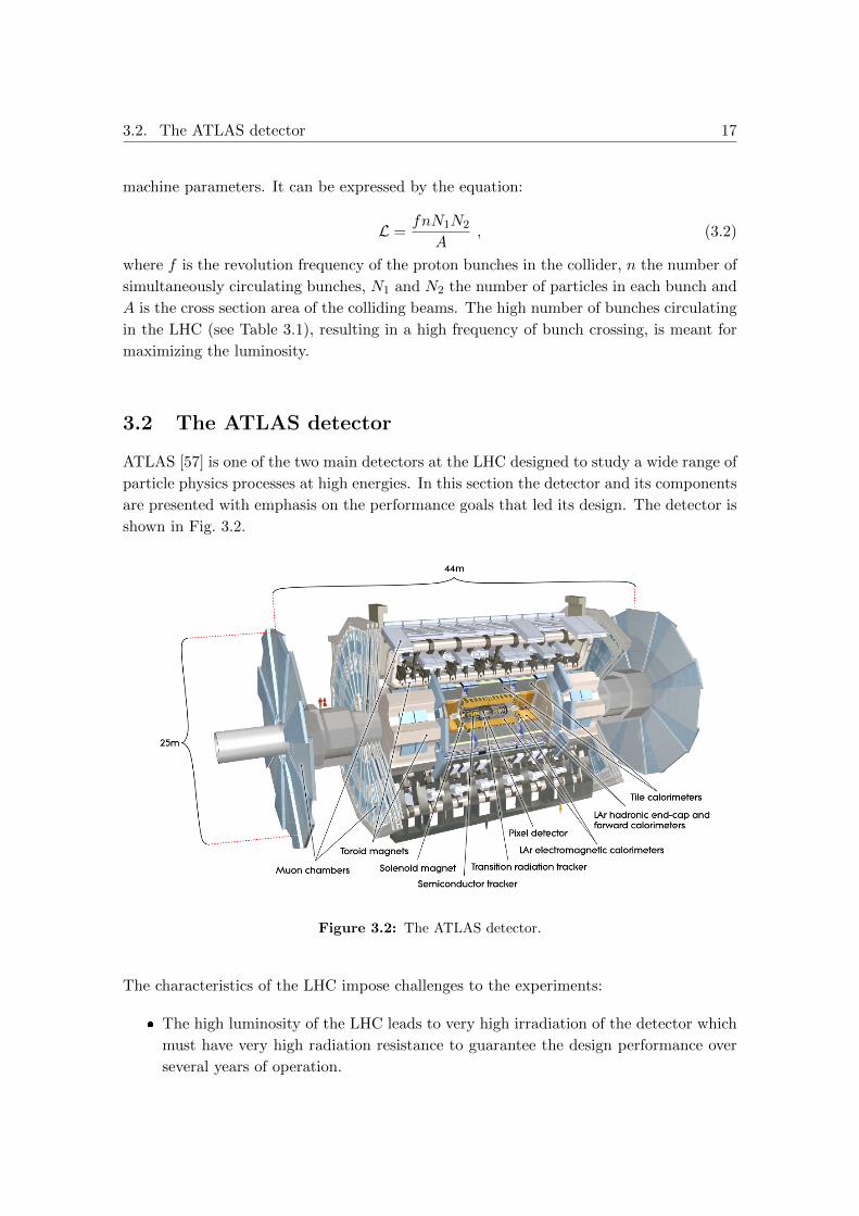
3.2 The ATLAS detector
ATLAS [57] is one of the two main detectors at the LHC designed to study a wide range of
particle physics processes at high energies. In this section the detector and its components
are presented with emphasis on the performance goals that led its design. The detector is
shown in Fig. 3.2.
Figure 3.2: The ATLAS detector.
The characteristics of the LHC impose challenges to the experiments:
The high luminosity of the LHC leads to very high irradiation of the detector which
must have very high radiation resistance to guarantee the design performance over
several years of operation.
18 Chapter 3. The ATLAS experiment at the Large Hadron Collider
The high density of protons per bunch at the LHC leads to an high number of soft
collisions happening in the same bunch crossing together with the hard process,
the so-called “pile-up”. Detectors operating at the LHC must be able to identify
and reconstructs particles and jets produced in hard scatterings which take place
together with several tens of such soft collisions.
The high interaction rate and particle density produced in the collisions require fast
and highly granulated detectors.
The physics goals of the ATLAS experiment lead to additional requirements on the detec-
tor:
Precise reconstruction of the primary vertex of the hard interaction even at the high
pile-up conditions.
A highly selective trigger system ensuring sufficient reduction of the data volume
with still high efficiency for the interesting processes.
Efficient particle reconstruction and identification and a precise measurement of
particle energies and of momenta.
Large solid angle coverage which is especially important for the reconstruction of
processes involving neutrinos and other new weakly interacting particles which can
only be observed by measuring the energy imbalance in the events.
Good energy resolution for electromagnetic showers in the calorimeters.
ATLAS consists of the following main elements:
The Magnet System, providing the magnetic field needed for the momentum mea-
surement of particle tracks is introduced in Section 3.2.2.
The Inner Detector, a tracking system operating in a solenoidal magnetic field, is
explained in Section 3.2.3.
The Calorimeter System used for the energy measurement of electromagnetically
(electrons and photons) and strongly interacting particles is described in Section 3.2.4.
The Muon Spectrometer, operating in a toroidal magnetic field and designed to iden-
tify muons and to measure their momentum is described in detail in Section 3.2.5 as
this thesis is particularly concerned with the performance of the muon reconstruction
in ATLAS.
The ATLAS Trigger System is described in Section 3.2.6.
The Luminosity Monitoring System providing the measurement of the luminosity
registered by ATLAS which is a key input for many physics analyses (see Sec-
tion 3.2.7).

3.2. The ATLAS detector 19
3.2.1 Notation and conventions
The coordinate system of ATLAS is defined in the following way (see [57]):
The origin is at the nominal interaction point.
The xy plane is transverse to the proton beams direction with:
– the y axis pointing upwards and
– the x axis pointing towards the centre of the LHC ring.
The z axis is oriented along the beam direction forming a right-handed coordinate
system.
Other important variables are defined in the following way:
θ is the azimuthal angle measured from the z axis.
Pseudorapidity is defined as η= −ln(tan( θ2)).
φ is the polar angle in the xy plane.
Transverse momentum pT and transverse energy ET are defined in the xy plane,
perpendicular to the beam axis.
Angular distance is measured by ∆R=√
∆η2 + ∆φ2.
Tracks are described by five parameters: cot(θ), φ, 1/pT , d0 and z0. d0 is the transverse
impact parameter, the distance of closest approach from the beam axis in the xy plane.
z0 is the longitudinal impact parameter, i.e. the z coordinate of the track at the point of
closest approach to the interaction point. The detector hemispheres for z > 0 and z < 0
are defined as side A and side C, respectively.
3.2.2 The Magnet System
The ATLAS Magnet System [57] (see Fig. 3.2) consists of four superconducting magnets:
A central solenoid with a length of 5.3 m and a diameter of 2.6 m provides a 2 T
magnetic field for the momentum measurement of charged particles tracks in the
Inner Detector.
A toroidal air-core magnet system provides a bending power of∫Bdl =2-8 Tm for
the muon spectrometer. It consists of a barrel and two endcaps magnets.
The barrel toroid consists of eight loops surrounding the calorimeters, with a length of
26 m and inner and outer diameters of 9.4 m and 20.1 m respectively. It covers the region
0 ≤ |η| ≤ 1.3 and provides a maximum field of 3.9 T. The endcap toroids are inserted into

20 Chapter 3. The ATLAS experiment at the Large Hadron Collider
the central one at the ends with a length of 5 m each, an outer diameter of 10.7 m and an
inner diameter of 1.7 m. They cover the regions 1.6 ≤ |η| ≤ 2.7 and provide a maximum
field of 4.1 T.
The bending power of the toroid system is reduced in the transition region between the
barrel and the endcaps, for 1.3 < |η| < 1.6.
3.2.3 The Inner Detector
The Inner Detector (ID) [57], shown in Fig. 3.3, is a tracking system for charged particles
in a solenoidal magnetic field. It consists of three sub-detectors:
the Pixel Detector,
the Semiconductor Tracker (SCT) and
the Transition Radiation Tracker (TRT).
The ID is 7 m long, has a diameter of 2.3 m, and covers the region 0 ≤ |η| ≤ 2.5. It has
a very high granularity, especially close to the interaction region where precise secondary
vertex reconstruction is needed for the identification of b-hadrons.
Figure 3.3: The Inner Detector.

3.2. The ATLAS detector 21
3.2.3.1 The Pixel Detector
The Pixel detector consists of silicon pixel sensors and provides three precision position
measurements along the track over the acceptance of 0 ≤ |η| ≤ 2.5. The barrel region
of the detector consists of three detector layers at radii of 5 cm, 9 cm, 12 cm from the
beam axis. The endcap regions consists of five disks each. The innermost layer (the B-
layer) is most important for the decay vertex reconstruction and is also most affected by
background radiation. The mechanical design of the detector allows for a substitution of
the B-layer during the 2013-14 LHC shutdown period.
The Pixel Detector provides position measurements with excellent intrinsic resolution of
10 µm in the Rφ and of 115 µm in the Rz plane [61].
3.2.3.2 The Semiconductor Tracker
The Semiconductor Tracker (SCT) consists of four double layers of silicon strip detectors
in the barrel and nine disk layers in the endcaps. In the barrel region the strips are
oriented parallel to the beam direction while in the endcaps they are oriented radially.
The detectors provide position measurements with an intrinsic resolution of 17 µm in the
Rφ plane and of 580 µm in the z direction in the barrel and in the radial direction for the
endcaps [61], covering the region 0 ≤ |η| ≤ 2.5.
3.2.3.3 The Transition Radiation Tracker
The Transition Radiation Tracker (TRT) consists of a large number of straw drift tubes
with a diameter of 4 mm assembled in 36 layers to provide on average 30 measurements
per track in the region |η| ≤ 2.5. The straw tubes operate with a Xe (70%) CO2(20%)
CF4 (10%) gas mixture. The detector measures tracks in the Rφ plane with a single tube
intrinsic resolution of 130 µm [61].
The TRT is also used for electron identification, especially at energies below 25 GeV. The
use of a xenon gas mixture makes it possible to detect transition-radiation photons which
are created in radiation sheets located between the straw tubes. The pion rejection factor
varies between 20 and 100 depending on η [61].
3.2.4 The Calorimeter System
The Calorimeter System [57] provides energy and position measurements for electrons,
photons and hadron jets. Furthermore it is essential for the reconstruction of hadronically
decaying τ leptons and for the measurement of the missing energy via energy imbalance
in the events, needed for the reconstruction of events with neutrinos or other weakly
interacting particles (see Section 4.6).
The Calorimeter System consists of an Electromagnetic (EM) Calorimeter covering the
region |η| ≤ 3.2 and of an Hadronic Calorimeter (HCAL) covering |η| ≤4.9.

22 Chapter 3. The ATLAS experiment at the Large Hadron Collider
Figure 3.4: The ATLAS Calorimeter System.
3.2.4.1 The Electromagnetic Calorimeter
The EM Calorimeter consists of a barrel part in the region |η| ≤ 1.475 and two endcaps
for 1.375 ≤ |η| ≤ 3.2. It is a sampling calorimeter with Liquid Argon (LAr) as active
medium in between accordion-shaped lead absorber plates. The region |η| ≤ 2.5 is used
for precision measurements and is segmented into three longitudinal regions:
A pre-shower layer, with a thickness of about 6 radiation lengths (X0) and readout
strips covering relative η angles between 0.003 and 0.25, depending on η itself, in
order to provide a high granularity in η. The size of the segmentation of this layer
is 0.1 in φ.
A middle section, with a thickness of about 16X0 and a readout segmented into
squares of ∆η × ∆φ = 0.025 × 0.025.
An outer layer, with an η depending thickness of 2-12X0 and a readout granularity
of ∆η × ∆φ = 0.050 × 0.025.
In addition in the region |η| < 1.8 a pre-sampling layer with a ∆η × ∆φ = 0.025 × 0.1
segmentation is used to estimate the energy loss of electrons and photons before the
calorimeters. In the region 2.5 < |η| ≤ 3.2 where electron and photon reconstruction
is not required, only two longitudinal samplings and a coarser granularity are sufficient to

3.2. The ATLAS detector 23
fulfil the required performance for jet energy and for energy imbalance measurements. In
the region 3.1 ≤ |η| ≤ 4.9, the Forward Calorimeter (FCAL), which is also using LAr
as active medium, provides both electromagnetic and hadronic shower measurements.
3.2.4.2 The Hadron Calorimeter
The Hadronic Calorimeter (HCAL) is a sampling calorimeter surrounding the EM Calorime-
ter and covering |η| ≤ 4.9 . It is divided into the following regions:
The barrel HCAL for |η| ≤ 1.7.
Two endcap HCALs for 1.5 ≤ |η| ≤ 3.2.
The Forward Calorimeter (FCAL) covers the region 3.1 ≤ |η| ≤ 4.9.
The barrel HCAL uses iron as absorber and scintillating tiles as active material. The
scintillation light is carried to photomultipliers by wave-length shifter (WLS) fibres. In
the most part of the calorimeter the granularity is ∆η × ∆φ = 0.10 × 0.10.
The two endcap HCALs use LAr as active material and copper plates as absorber. They
are divided into two wheels, the first one with 25 mm thick copper plates and the second
one with 50 mm thick plates. The 8 mm wide gap between consecutive plates is equipped
with three parallel electrodes, where the central one is the readout layer and the others
carry the high voltage.
The FCAL works in a very high radiation environment which represents a challenge for
the detector design. It uses LAr as active medium and copper and tungsten as absorber
materials. The calorimeter consists of a metal matrix with longitudinal channels in which
metal rods are inserted.
An important characteristics of the HCAL is its hermeticity. Its thickness is greater than
10 hadronic interaction lengths λ over the whole acceptance ensuring a good resolution
for the jet energy and for the momentum imbalance measurements and low hadron punch-
through into the muon system.
3.2.5 The Muon Spectrometer
The ATLAS Muon Spectrometer (MS) [57] is designed for the reconstruction of muons
and the measurement of their momentum either as a stand-alone system or in combination
with the Inner Detector. Due to the importance of muons for the analyses in this thesis,
the MS design is discussed in detail below.
The Muon Spectrometer shown in Fig. 3.5 covers the region |η| ≤ 2.7 with a small gap at
|η| = 0 used for cables and services belonging to the Inner Detector and to the Calorimeter
systems. The following regions of the spectrometer can be distinguished:

24 Chapter 3. The ATLAS experiment at the Large Hadron Collider
The barrel region covering |η| ≤ 1.05 with the central region at |η| < 0.1.
The endcap regions covering 1.05 < |η| ≤ 2.7 with the transition regions between
barrel and endcaps at 1.05 < |η| < 1.3 and the forward regions at |η| > 2.0.
The MS operates in the magnetic field of the toroid magnets described in Section 3.2.2.
The field bending plane is the Rη plane.
The MS uses four different types of muon chambers for muon reconstruction:
Monitored Drift Tube (MDT) chambers provide position measurement in the bend-
ing plane over most of the MS acceptance region.
Cathode Strip Chambers (CSC) provide position measurement both in the bending
and in the non-bending plane in the innermost detector layer of the forward regions.
Resistive Plate Chambers (RPC) are used for trigger information and for non-
bending plane position measurement in the barrel region.
Thin Gap Chambers (TGC) are used for trigger information and non-bending plane
position measurement in the endcap regions.
In the following the position in the bending plane will be referred to as the precision co-
ordinate and the position in the non-bending plane as the transverse coordinate.
In the barrel region the precision MDT chambers are arranged in three layers with cylin-
drical symmetry around the beam axis providing the three track position measurements
needed for momentum determination:
The inner (I) layer at R=5 m.
The middle (M) layer at R=7.5 m.
The outer (O) layer at R=10 m.
In the endcaps chamber layers are located at 7 m (I), 14 m (M) and 21-23 m (O) from the
nominal interaction point.
The chambers are arranged in polar octants, each divided into two sectors, one with larger
chambers (large sector) and one with smaller chambers (small sector). The MS layout is
shown in Fig. 3.5. The small and large chambers partially overlap to ensure full spatial
coverage and allow for relative alignment with tracks.
The expected muon momentum resolution is shown in Fig. 3.6 as a function of the muon
transverse momentum pT. In the low and medium pT region, the multiple scattering and

3.2. The ATLAS detector 25
Figure 3.5: Cross section views of the ATLAS Muon Spectrometer in the non-bending plane(top) and in the bending plane (bottom).
energy loss fluctuations dominate, while in the high pT region the chamber spatial resolu-
tion and the alignment of the chambers are the main effects determining the momentum
resolution.
3.2.5.1 Monitored Drift Tube chambers
Monitored Drift Tube (MDT) chambers provide precision position measurement in the
bending plane over most of the solid angle covered by the Muon Spectrometer. 1150

26 Chapter 3. The ATLAS experiment at the Large Hadron Collider
Figure 3.6: Contributions to the muon momentum resolution of the ATLAS Muon Spectrometeras a function of the muon transverse momentum [61].
chambers are operating in the spectrometer.
A MDT chamber is composed of drift tubes, with a length of 1-6 m, organized in two
multilayers separated by a spacer; each multilayer is composed of 3 or 4 layers of tubes
(see Fig. 3.7).
The tubes are operated with Ar/CO2(93/7) gas at a pressure of 3 bar. The walls of the
tubes are grounded. A voltage of 3080 V is applied to the central wire. In Fig. 3.7 an
illustration of the operation mechanism of a drift tube is shown. When a charged particle
is crossing the tube, it produces electron-ion pairs along its path (primary ionization).
The electric field inside the tube causes the electrons to drift to the wire. Close to the
wire the ionization electrons are sufficiently accelerated to produce new electron-ion pairs
in a so-called avalanche process (secondary ionization). The multiplication factor (gain)
of the device, which depends on the voltage applied, on the gas pressure and on the tube
diameter, has been chosen to be 2·104, sufficiently low to prevent streamers and to avoid
ageing of the drift tubes. The drift of the electrons to the wire and of the ions to the tube
walls induces an electric signal on the wire. This signal is used to measure the electron drift
time with respect to the time the muon passes the tube, i.e. the proton bunch crossing
time corrected for the muon time of flight.
The drift time measurement is then converted into the distance of smallest approach of

3.2. The ATLAS detector 27
Figure 3.7: Layout of a Monitored Drift Tube chamber (left) and working principle of a drifttube (right).
the muon trajectory to the wire using the r-t relation, which is specific for the gas mixture
and is determined depending on temperature and magnetic field strength. The muon track
is fitted to the corresponding drift circles. Further details about the muon reconstruction
are given in Section 4.7.
3.2.5.2 Cathode Strip Chambers
Cathode Strip Chambers (CSC) are multi-wire proportional chambers with readout cath-
ode strips parallel and orthogonal to the wires used in the innermost layer of the 2.0 ≤ |η| ≤ 2.7
region of the MS, where the high background radiation rate would degrade too much the
performance of the MDT chambers. The layout of the CSC is shown in Fig. 3.8.
Figure 3.8: Schematic layout of a Cathode Strip Chamber.
CSC chambers operate with a Ar/CO2/CF4(30/50/20) gas. The wires are at a potential
of 2600 V. Charged particle crossing a CSC plane generate ionization charges which are
multiplied by an avalanche process near the wires. The precision coordinate is determined

28 Chapter 3. The ATLAS experiment at the Large Hadron Collider
as the mean of the orthogonal strip cathode coordinates weighted by the charge signals
induced on them, with a resolution of about 60 µm for a single CSC plane. Each chamber
is composed of 4 planes. The transverse coordinate is measured with a resolution of about
5 mm by the cathode strips oriented parallel to the wires, which have larger pitch.
The CSC chambers are designed to operate with a background radiation level up to
1000 Hz/cm2, which is sufficient to cope with the working conditions of the inner part
of the forward spectrometer region.
3.2.5.3 Alignment system for the precision chambers
MDT and CSC chambers are installed with millimetre precision, but their positions must
be known with a relative accuracy of 30 µm in order to reach the muon momentum
resolution. To achieve this, the following strategy is used:
Straight muon tracks are used to measure the relative chamber positions when the
toroidal magnetic field is turned off.
An optical alignment monitoring system connects the chambers in projective towers
with respect to the interaction point and allows for the measurement of their relative
movements with micrometer precision.
Further information can be found in [62] and [63].
3.2.5.4 Resistive Plate Chambers
Resistive Plate Chambers (RPC) are composed of two independent detector layers, each
providing two-dimensional coordinate measurements. The layers consists of two Bakelite
plates of 2 mm thickness separated by a 12 mm wide gap. The readout is provided by
η cathode strips for the bending plane measurement and by φ strips for the non-bending
plane measurement. They operate with C2H2F4/C4H10(97/3).
RPCs have a typical spatial resolution of 1 cm. Their excellent time resolution of 1 ns
allows for their use as muon trigger chambers in the barrel region with identification of
the bunch crossing from which the muon originates. They are arranged in three layers,
two of them below and above the middle MDT layer and the third one at the outer MDT
layer (see Fig. 3.5).
The first and the second RPC layers from the beam pipe are used for low-pT muon triggers
while the larger level arm between the middle and outer layers enables high pT triggers.
3.2.5.5 Thin Gap Chambers
Thin Gap Chambers (TGC) are multi-wire proportional chambers with anode wire pitch
larger than the anode-cathode distance which are operated in a CO2/C5H12 gas mix-
ture. The wires provide the coordinate measurement in the bending direction while the

3.2. The ATLAS detector 29
transverse coordinate measurement is provided by the cathode strips orthogonal to the
wires.
Seven TGC planes are placed in the middle layer and two in the inner layer of the MS
endcap regions. They are used to provide the trigger signals and the non-bending plane
measurement in these regions.
3.2.6 The Trigger System
At design luminosity, the rate of proton-proton interactions is about 1 GHz. Most events
are not interesting for physics analyses. The information stored for an event in ATLAS
requires on averages 1.3 megabytes of disk space. Thus a trigger system with an high
selective power is necessary to select the events that will be recorded at an acceptable
rate. A three level trigger system [57] has been designed for the ATLAS experiment:
The first-level (L1) trigger is completely hardware based and uses partial information
of the event to reduce the data rate to 75 kHz.
The second-level (L2) trigger uses almost complete event information to reduce the
rate to 3.5 kHz.
The event filter (EF) analyses the full event information to finally reduce the rate
to 200 Hz.
The EF performs a reconstruction of the physics objects (which is different from the final,
offline reconstruction) and applies kinematic requirements. Many different EF level trigger
conditions are used in parallel and the ones with softer cuts may have to be prescaled to
ensure that the final output rate does not exceed the sustainable 200 Hz. The final rate
corresponds to 300 megabytes of data per second to be stored on disk.
3.2.6.1 The first-level muon trigger system
The first-level muon trigger uses the Resistive Plate Chambers and Thin Gap Chambers
described in Sections 3.2.5.4 and 3.2.5.5. These chambers have high time resolution suffi-
cient to unambiguously identify the bunch crossing a muon track is belonging to.
As illustrated in Fig. 3.9, the trigger algorithm is based on the concept of trigger roads:
a first-level muon trigger results if there are hits in two, for the low-pT trigger in the
6-9 GeV range, or three, for the high-pT trigger in the 9-35 GeV range trigger chamber
layers within roads of width depending on the pT threshold. The muon trigger system
covers the region |η| ≤ 2.4.

30 Chapter 3. The ATLAS experiment at the Large Hadron Collider
Figure 3.9: Concept and layout of the first-level muon trigger system.
3.2.7 Luminosity measurement in the ATLAS experiment
In order to determine the cross section of a physics process from the measured event rate
according to Eq. 3.1 the corresponding integrated luminosity recorded by the ATLAS de-
tector has to be measured as well. The main luminosity detector used in ATLAS is LUCID
(Luminosity measurement using Cerenkov Integrating Detector) [64]. It consists of sixteen
drift tubes of 15 mm diameter filled with C4F10 gas and arranged around the beam pipe
covering the 5.6 ≤ |η| ≤ 6.1 angle. It is very resistant to radiation, as it has to work
in a highly irradiated environment. Two LUCID detectors are symmetrically placed at
z = ± 17 m from the interaction point.
The LUCID detector provides a measurement of the rate of inelastic collisions per bunch
crossing detecting the Cerenkov photons emitted by charged particles produced in inelastic
proton-proton interactions. The luminosity is calculated using this rate and the beam
parameters calibrated with van der Meer scans as described in [64].

Chapter 4
Reconstruction of physics objects
In this chapter the algorithms used to reconstruct the trajectories and energies of different
types of particles, hadron jets and other observables needed for the data analysis in this
thesis are described.
4.1 Detector simulation
An introduction to Monte Carlo generators and to the simulation of physics processes has
been given in Chapter 2. In order to compare data and simulation also the response of
the ATLAS detector to the particle interactions has to be simulated taking into account
the data taking conditions. The simulation proceeds in the following steps:
A physics process is simulated by a Monte Carlo generator (generator level).
The detector response to the generator level particles is simulated using the GEANT 4
software [65] (detector simulation level).
Digitisation of the detector signals is performed providing output in the same form
of the detector readout electronics. Pile-up and radiation background simulations
are added in this step (digitisation level).
The output of the digitisation is used to reconstruct physics objects by the same
algorithms as used for data (reconstruction level).
The pile-up effect briefly introduced in Section 3.2 is caused by soft proton interactions
recorded by the detector in the same event with a triggered hard scattering process. There
are two main sources of pile-up:
In-time pile-up is caused by multiple proton-proton interactions in a bunch crossing
due to the high proton density in the bunches. Data used in this thesis are collected
with up to 24 proton-proton interactions per bunch crossing [66].
31

32 Chapter 4. Reconstruction of physics objects
Out-of-time pile-up occurs because the readout electronics of many detectors inte-
grates over several bunch-crossing. This effect depends on the time interval between
bunches.
The main pile-up effects occur in the calorimeters where in-time pile-up increases the
measured energies while out-of-time pile-up may decrease the observed energy due to the
negative energy tails in the LAr pulse shaping.
In the digitisation step of the detector response simulation, pile-up events are added to
the simulated physics events depending on the data taking conditions. Since simulated
events are often produced before the data taking, reweightings of the Monte Carlo events
according to the pile-up level measured in data is applied. The parameter used for the
reweighting is the average number of interactions per bunch crossing < µ > in a given
luminosity block, which usually represents a minute of data taking.
4.2 Charged particle and vertex reconstruction in the Inner
Detector
The track reconstruction in the ID is performed in three steps [67]:
In the pre-processing stage hit clusters are formed starting from the Pixel and SCT
detectors. SCT clusters are transformed into space-points combining hits from the
opposite sides of the SCT modules. TRT drift times are transformed into drift circles
with the same technique as used for the MDT chambers (see Section 3.2.5.1).
At the track-finding stage track-seeds are generated starting from the internal track-
ing layers and then extended through SCT and TRT associating clusters and hits to
them. Finally, a full track fit is performed.
In the post-processing stage the reconstruction of the primary vertex of interactions
is performed, followed by secondary vertex reconstruction and photon conversion
identification.
To allow for a quality assessment of reconstructed tracks, information about track holes
(silicon sensors crossed by a track which have no hits) and outliers (TRT hits with large χ2
contribution during the track-finding stage) are stored. The expected transverse momen-
tum resolution for ID tracks is 2-5% for low pT tracks and 4-15% for medium pT tracks
up to 100 GeV, strongly depending on |η| (see Fig. 4.1). The measurement of the track
reconstruction efficiency will be discussed in the next chapter.
Tracks are associated to common vertices, and the primary interaction vertex is identified
as the vertex with highest∑
pT2 of the associated tracks. The tracks are then refitted
using the selected primary vertex. As a figure of merit, the reconstruction efficiency for the
hard scattering interaction vertex is predicted to be above 99% in simulations for Z → ee
and Z → µµ decays even in very high pile-up conditions [68].

4.3. Electrons and Photons 33
Figure 4.1: Expected 1/pT resolution of ID tracks as a function of η of the tracks for simulatedpT=1, 5, 10 GeV muon tracks [61].
4.3 Electrons and Photons
An efficient identification and reconstruction of electrons and photons as well as precise
measurement of their energy is an important feature of the ATLAS detector in order to
fulfil the demanding requirements of the physics program. The goal is challenging because
of the working conditions of the LHC and because of the relatively large amount of mate-
rial of the tracking detectors in front of the electromagnetic calorimeters.
Three algorithms are used for the reconstruction of electrons and photons [69, 70]:
A energy cluster-seeded method is used as the standard reconstruction algorithm.
A track-seeded algorithm is used for low-pT electrons.
A dedicated algorithm is used for electrons in the forward region (2.5 < |η| < 4.9)
which is not covered by the Inner Detector.
For the purpose of this thesis only the first algorithm is described.
4.3.1 Electron reconstruction
The standard electron reconstruction is seeded by an EM calorimeter cluster consisting of
energy deposits of ET >2.5 GeV in an 3x5 group of calorimeter cells in η and φ. The cluster
is then matched to ID tracks within a ∆η = 0.05 window and a ∆φ window of 0.1 on the
side of the track to which it is bending and of 0.05 on the other side [71]. This asymmetry
in the ∆φ window takes into account the effects of bremsstrahlung. EM clusters matched
to ID tracks are electron candidates. The calorimeter cluster is then recomputed using 3x7

34 Chapter 4. Reconstruction of physics objects
cells in the barrel and 5x5 cells in the endcaps. The energy of the electron is corrected for
the estimated energy loss of the particle in the material outside the calorimeter. The energy
of the electron is determined using calorimeter cluster information. For the direction of
the electron, ID track information is used for tracks with silicon detectors hits and clusters
information otherwise.
The reconstructed electrons are classified in three categories, loose, medium and tight,
using several quality criteria (see [71]): among others, the agreement between ID and
calorimeter measurements and the numbers of hits in the different ID subdetectors. The
expected jet rejection rates in the three categories are about 500, 5000 and 50000 respec-
tively. This classification has been improved for 2011 and 2012 data taking with the new
quality categories loose++, medium++, tight++.
The performance of the electron reconstruction from 2011 measurements is shown in
Fig. 4.2. The agreement of the measured reconstruction efficiencies in data and simu-
lations is very good. The electron momentum resolution in the simulations is adjusted
such that the simulated dielectron invariant mass distribution in simulated Z → ee events
matches the data.
Figure 4.2: Measured electron reconstruction efficiency as a function of the number of recon-structed vertices in the events (left) and electron-positron invariant mass distribution in Z → eedecays (right) for 2011 data and Monte Carlo simulation [72].
4.3.2 Photon reconstruction
Reconstructed photons are divided into two categories: converted photons and unconverted
photons.
Reconstructed unconverted photons are seeded by EM clusters like the electron candidates,
but have no matching ID track. For photons converting into electron-positron pairs inside
the ID, the reconstruction relies on the identification of conversion vertices, with two or
even only one associated track, the latter case happening when the two conversion electrons
are too close to be distinguished or when one of the two tracks, usually with very low pT,
is not reconstructed. Tracks from conversion vertices matched to calorimeter clusters like

4.4. Jets 35
for the electron reconstruction are converted-photon candidates.
Many converted photons are also selected as electron candidates. A recovery procedure
for these photons described in [69] is applied.
The photon reconstruction performance expected from simulations is shown in Fig. 4.3.
After the recovery procedure on photons the predicted photon reconstruction efficiency is
very high.
Figure 4.3: Expected photon reconstruction efficiency as a function of η [70].
4.4 Jets
Jets are collimated bunches of hadron tracks and their decay particles which at high-energy
hadron colliders are by far dominating the event final states.
4.4.1 Jet Reconstruction
The baseline method for jet reconstruction in ATLAS [73] is the anti-kT algorithm [74].
The reconstruction starts with a topological clustering algorithm searching for a calorime-
ter seed cell with a signal-to-noise ratio S/N > 4. Neighbouring cells with a S/N > 2 are
consecutively added. Local maximums in cell energies are located and spilt off to form the
seeds for separate clusters.
The iterative anti-kT algorithm starts with the identification of pseudo-jets, either par-
ticle 4-momenta in Monte Carlo simulations or calorimeter clusters in data. It uses the
definitions:
dij = min(1
k2T i
,1
k2Tj
)∆2ij
R2(4.1)

36 Chapter 4. Reconstruction of physics objects
and
di =1
k2T i
, (4.2)
where the indices i,j run over all pseudo-jets, kT is the transverse momentum of a given
pseudo-jet, ∆ij =√
∆y2ij + ∆φ2
ij the angular distance between two pseudo-jets and R a
η-φ distance parameter with values 0.4 or 0.6 used as baseline in ATLAS.
For a given number of pseudo-jets N , the smallest of all dij and di variables is determined
with i, j = 1, ..., N . The pseudo-jet i for minimum variable di is identified as a jet and
removed from the list of pseudo-jets. Otherwise, if dij is the minimum variable, pseudo-
jets i and j are recombined. The reconstruction procedure iterates until there are no
pseudo-jets left. With this algorithm the hardest particles lead the merging procedure
and softer particles around them will be merged with them, until the final jets are formed.
The anti-kT algorithm is infrared safe [74], i.e. the eventual presence of soft particles
between two hard particles does not affect their reconstruction as a single jet. It is also
collinear safe [74], i.e. a jet is reconstructed without differences when a certain part of its
momentum is carried by a single particle or if the same amount is carried in total by two
or more collinear particles.
4.4.2 Jet quality
Jets originating from proton-proton scattering must be distinguished from non-collision
background due to cosmic muons, noise, or interactions of the beam protons with residual
gas molecules in the beam-pipe or with inactive detector and shielding material. For this
purpose, many jet parameters are used to classify the jets in terms of cleanliness as tight,
medium, loose jets [73] as well as jets failing even the loose requirements. A further still
looser category has been introduced as the standard for the 2011 physics analyses [75].
4.4.3 Jet energy measurement
The jet energy calibration relates the energy deposition measured by the calorimeters to
the true energy of a jet. In Monte Carlo simulations the correction factors are determined
by comparison with truth jets, which are reconstructed from the stable particles generated
using the same anti-kT algorithm as for final state jets. For the real data the calibration
is performed using test-beam studies.
The initial energy calibration is be performed with respect to different energy scales [73]:
the EM scale corresponding to the response of the calorimeters to the electromag-
netically interacting components of a jet and
the local cluster weighting (LCW) scale which relies on the identification of energy
clusters in a jet and their classification as hadronic or electromagnetic clusters, for
which different calibration corrections are applied.

4.4. Jets 37
A third calibration scale, the global calorimeter cell weighting (GCW) scale is not relevant
for the purpose of this thesis.
In addition to the calibration, a Jet Energy Scale (JES) correction is applied to obtain
a final result as close as possible to the true energy of a jet, including corrections for
pile-up effects and for the position of the primary interaction vertex of the event and
simulation-based corrections.
The standard jet calibration used in this thesis is the EM+JES scheme. In Fig. 4.4 a
measurement of the jet energy resolution is shown, which is performed by studying the
pT balance of events with a Z boson and one reconstructed jet, in which the jet momentum
is expected to balance the one of the Z boson. The width of the distribution of the ratio
of the transverse momenta of the jet and of the Z boson is used to compare the jet pT
resolution in data and in simulations, finding a good agreement.
Figure 4.4: Measurement of the resolution of the jet pT relative to pTref of the Z boson in Z +
1-jet events as a function of pTref [76].
4.4.4 Heavy flavour jet tagging
Jets originated by the hadronization of heavy flavour quarks (i.e. charm and bottom
quarks) can be identified relying on the properties of b and of c hadrons. The long lifetimes
and heavy masses of these hadrons produces signature that can be used to discriminate
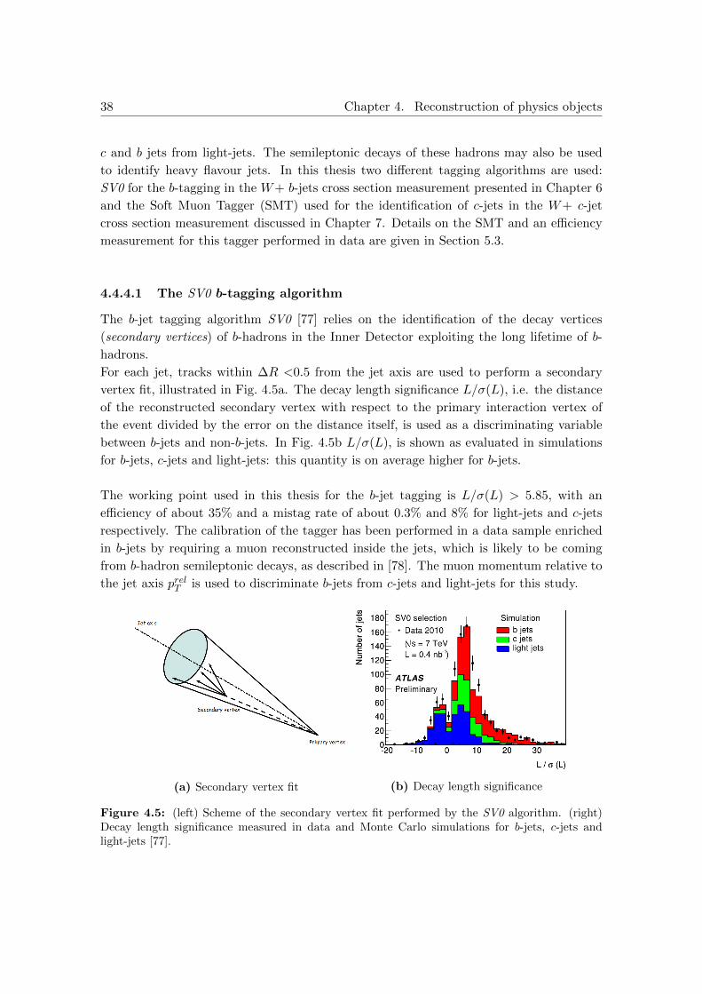
38 Chapter 4. Reconstruction of physics objects
c and b jets from light-jets. The semileptonic decays of these hadrons may also be used
to identify heavy flavour jets. In this thesis two different tagging algorithms are used:
SV0 for the b-tagging in the W+ b-jets cross section measurement presented in Chapter 6
and the Soft Muon Tagger (SMT) used for the identification of c-jets in the W+ c-jet
cross section measurement discussed in Chapter 7. Details on the SMT and an efficiency
measurement for this tagger performed in data are given in Section 5.3.
4.4.4.1 The SV0 b-tagging algorithm
The b-jet tagging algorithm SV0 [77] relies on the identification of the decay vertices
(secondary vertices) of b-hadrons in the Inner Detector exploiting the long lifetime of b-
hadrons.
For each jet, tracks within ∆R <0.5 from the jet axis are used to perform a secondary
vertex fit, illustrated in Fig. 4.5a. The decay length significance L/σ(L), i.e. the distance
of the reconstructed secondary vertex with respect to the primary interaction vertex of
the event divided by the error on the distance itself, is used as a discriminating variable
between b-jets and non-b-jets. In Fig. 4.5b L/σ(L), is shown as evaluated in simulations
for b-jets, c-jets and light-jets: this quantity is on average higher for b-jets.
The working point used in this thesis for the b-jet tagging is L/σ(L) > 5.85, with an
efficiency of about 35% and a mistag rate of about 0.3% and 8% for light-jets and c-jets
respectively. The calibration of the tagger has been performed in a data sample enriched
in b-jets by requiring a muon reconstructed inside the jets, which is likely to be coming
from b-hadron semileptonic decays, as described in [78]. The muon momentum relative to
the jet axis prelT is used to discriminate b-jets from c-jets and light-jets for this study.
(a) Secondary vertex fit (b) Decay length significance
Figure 4.5: (left) Scheme of the secondary vertex fit performed by the SV0 algorithm. (right)Decay length significance measured in data and Monte Carlo simulations for b-jets, c-jets andlight-jets [77].
4.5. τ leptons 39
4.5 τ leptons
τ leptons are unstable particles decaying into hadrons with a branching ratio BR = 65% [25]
and leptons with BR = 35% [25]. Due to their short lifetime, corresponding to a mean
free path of about 100 µm, their leptonic decays cannot be distinguished from prompt
electrons and muons. The reconstruction of hadronic τ decays and their distinction from
QCD jets is challenging. It uses properties of the hadronic τ decays such as the low
track multiplicity and the narrow collimation of the tracks and energy depositions in the
calorimeters. A description of the hadronic τ decay reconstruction is given in [61].
4.6 Transverse missing energy
The signature of long-lived or stable weakly interacting particles like neutrinos in the
detector is missing transverse energy EmissT , i.e. the energy imbalance in the transverse
plane due to not detected particles. The transverse energy imbalance is used because at
a hadron collider the energies of the colliding partons in the hard parton scattering are
not known for each event and many soft collision products leave the detector undetected.
EmissT is determined as the negative sum of the transverse energies of all final state particles
ET . The energy Ex,y in the transverse coordinates x, y is reconstructed in ATLAS [79] by
summing up the following contributions:
Ex,y =Eelectronsx,y + Ephotonsx,y + Eτ leptonsx,y + Emuonsx,y + Ejetsx,y
+ Esoft jetsx,y + Ecalo µx,y + Ecell outx,y .(4.3)
Ejetsx,y and Esoft jetsx,y are determined from calorimeter cells in clusters associated to jets
with calibrated pT > 20 GeV and 7 GeV < pT < 20 GeV respectively. Ecell outx,y is the
sum of calorimeter cells energies in clusters not associated to jets or particles. Emiss,calo µx,y
is the energy loss of muons in the calorimeters. It is evaluated with different methods
for isolated and non-isolated muons and only added in the second case to avoid double
counting (see details in [79]).
Figure 4.6 shows the measured EmissT distribution in Z → µµ events. Data and simulation
are in good agreement with each other.
4.7 Muons
Muons are produced in many important physics processes. The detector signature for
muons is very clean and therefore the misidentification rate is very low. Furthermore the
Muon Spectrometer described in Section 3.2.5 detects muons with very high efficiency and
momentum resolution. A detailed study of the muon spectrometer performance is pre-
sented in next chapter. In this section, the basic strategies used for muon reconstruction

40 Chapter 4. Reconstruction of physics objects
Figure 4.6: Distribution of the EmissT in Z → µµ events in data and simulation [80].
are discussed.
Two groups of algorithms (chains) are used for muon reconstruction in ATLAS, Muid [81]
and Staco [82]. Both chains include several muon reconstruction algorithms using either
the muon spectrometer information only (stand-alone reconstruction, SA), combining ID
and MS tracks (combined reconstruction, CB), or identifying ID tracks as muons using
partial muon spectrometer information (segment tagged reconstruction, ST).
For the stand-alone muon reconstruction, both chains start from single hits in the preci-
sion chambers, combining them into track segments. Muon spectrometer tracks are re-
constructed connecting the segments and extrapolating the track to the beam line, taking
into account multiple scattering and energy loss in the detector elements. The stand-alone
reconstruction covers |η| ≤ 2.7, with acceptance gaps at |η| < 0.1 and |η| ≈ 1.2 for the
passage of services.
The combined muon reconstruction starts from an ID track and a stand-alone muon spec-
trometer track to produce a combined track. The Muid combined algorithm performs a
refit of the total track, while the Staco algorithm combines the parameters of the two
tracks statistically. The coverage of the combined reconstruction is reduced to the region
|η| ≤ 2.5 due to the Inner Detector acceptance, with the same gaps at |η| < 0.1 and
|η| ≈ 1.2 as for the stand-alone reconstruction. A measure of the quality of the track
combination is provided by the parameter
χ2match = (TMS − T ID)T (CMS +CID)−1(TMS − T ID) (4.4)
where T is a vector of the five track parameters defined in Section 3.2.1 and C the corre-

4.7. Muons 41
sponding covariance matrix.
The segment tagged muon reconstruction identifies ID tracks as muons if they can be
associated to segments in the muon spectrometer. This method is useful for low pT muon
tracks, which do not reach the layers of the muon spectrometer due to bending in the
magnetic field, or in the regions |η| < 0.1 and |η| ≈ 1.2 where tracks may pass through
only one or two layers of chambers. This reconstruction strategy has a slightly higher
fake rate but improves the muon efficiency for the reconstruction of final states with many
muons, in particular from Higgs and SUSY decays.
In addition to the three muon categories, calorimeter tagged muons are identified as ID
tracks which are associated to energy deposits in the calorimeters compatible with that
of minimum ionizing particles. This type of muon candidates recovers efficiency in the
|η| < 0.1 region where the MS coverage is reduced.
The muon reconstruction efficiency of the MS starts from zero at pT ≈ 2.5 GeV and
reaches its plateau at pT ≈ 6 GeV [61]. In Fig. 4.7 the dimuon invariant mass resolution
measured in Z → µµ events using combined muon reconstruction in the 2011 data is
shown for different η regions. Additional smearing of the muon momentum resolution in
simulation is applied to correct for the observed disagreement with the data in the mµµ
resolution.
Figure 4.7: Dimuon invariant mass resolution measured in Z → µµ events using combined muonreconstruction in 2011 data and simulations [83].

42 Chapter 4. Reconstruction of physics objects
4.8 Track and calorimeter isolation
For many physics analyses the isolation of physics objects (e.g. muons) is a powerful
discriminating variable to reject QCD background. Two kinds of variables are used to
measure the isolation:
Track isolation uses the sum of the pT of all ID tracks reconstructed in a cone
with a given radius ∆R with respect to an object.
Calorimeter isolation uses the sum of the energy deposits in the calorimeters in
a cone around the object with a radius ∆R.
Standard cone radii for the isolation requirements in ATLAS are ∆R = 0.1, 0.2, 0.3, 0.4.

Chapter 5
Muon reconstruction performance
Essential for all physics analyses is the understanding of the detector performance under
real data taking conditions. A tremendous effort has been put into the measurement and
monitoring of the performance of the ATLAS detector in order to correct the detector
response in the Monte Carlo simulations to fit the data.
Leptonic decays of W and Z bosons are natural candidates for the study of the muon sys-
tem performance, since they provide clean samples of muons with high cross sections. The
dimuon decays of Z bosons in particular offer a very clear signature which allows for effi-
cient background rejection. The resulting sample of muons is used for many performance
studies. In this chapter, measurements of the muon reconstruction and identification
efficiencies using the so-called “Tag-and-Probe” method in Z → µµ events are discussed.
5.1 Measurement of the muon reconstruction efficiency
Monitoring of the muon reconstruction efficiency during data taking is an important ver-
ification of the detector performance. Furthermore, the results are needed to correct the
simulated detector response in Monte Carlo simulations to correctly reproduce the perfor-
mance in data.
The correction is performed by evaluating the efficiency ε in data and in Monte Carlo and
using the correction scale factor
SF =εDATAεMC
(5.1)
to reweight the simulated events. The results of this section are for the 2011 ATLAS data
set used in this thesis. In Appendix B, the results for the 2012 data set are shown.
5.1.1 Dependence on the Muon Spectrometer regions
For the efficiency measurement, the Muon Spectrometer is subdivided into ten regions
according to the coverage provided and to the detector technologies and alignment system
43

44 Chapter 5. Muon reconstruction performance
used. The SFs are determined separately for the ten regions, assuming that they are
constant in each region.
Figure 5.1: Muon Spectrometer regions in the η-φ plane.
The ten regions are defined in the following way (see the illustration in Fig. 5.1):
The barrel is divided into three regions corresponding to large and small chamber
sectors and the overlap between them.
In the feet region of the barrel the geometrical acceptance of the spectrometer is
degraded due to the presence of the steel feet supporting the ATLAS detector.
The transition region between barrel and endcap is around η = 1.1.
The two endcap regions, defined up to |η| = 2.0, are divided into large and small
chamber sectors.
The BEE region of the endcaps uses extra barrel (BEE) chambers mounted on the
endcap toroid cryostat which are not connected to the optical alignment system.
The CSC or forward region (|η| >2.0) is covered by the CSC chambers in the inner-
most endcap layer and is divided into large and small chamber sectors.
Large and small sectors are treated separately because of the different connection to the
alignment system (see [62, 63]).
5.1.2 The Tag-and-Probe method
The so called Tag-and-Probe method uses Z → µµ events to measure the muon recon-
struction efficiency. One of the muons from the Z → µµ decay fulfilling tight requirements,
i.e. a well reconstructed combined muon (see Section 4.7), is used as a tag muon, while

5.1. Measurement of the muon reconstruction efficiency 45
the second one, fulfilling looser requirements, is used as a probe muon. When a tag and
probe muon pair is found with an invariant mass (mZ −10 GeV) < mµµ < (mZ + 10 GeV)
the event is identified as a Z → µµ event. Tighter selection criteria are then applied on
the probe muon and the efficiency of this tighter selection is determined as the fraction of
probe muons passing the tighter cuts. The Tag-and-Probe method is applied
to evaluate the muon reconstruction efficiency in the Muon Spectrometer (MS), by
using an Inner Detector (ID) track or a calorimeter tagged muon as probe and
calculating the fraction of probes matching a fully reconstructed muon and
to evaluate the ID reconstruction efficiency by using a MS track as probe and cal-
culating the fraction of probes matching an ID track.
Other possible applications are described later in this chapter.
The efficiency of stand-alone (SA) muon reconstruction is determined using the first
method, while for combined (CB) and segment tagged (ST) muons which use both Muon
Spectrometer and Inner Detector information the total reconstruction efficiency is given
by
εreco = εMSreco · εcombination · εIDreco . (5.2)
Using ID tracks as probes and matching them to CB or ST muons the εMSrecoεcombination
term can be determined. For calorimeter tagged muons, which do not use spectrometer
information, the same strategy as for ID tracks is applied.
The statistical error on the measured efficiency is determined in the following way. The
number k of events with unmatched probe, i.e. in which the reconstruction of the probe
as muon fails, follows a Poissonian distribution. The mean value of k is N(1 − ε) and
its variance σ(k) =√k =
√(1− ε)N , where N is the total number of probe muons.
Therefore the error on the efficiency is:
σ(ε) = σ(1− ε) =
√1− εN
. (5.3)
The estimate fails for ε = 1 but is applicable in all practical cases with ε < 1.
5.1.3 Data and Monte Carlo samples
For the analysis the full 2011 ATLAS data set, corresponding to 4.7 fb−1 of luminosity,
was used. It is divided into data taking periods with uniform detector performance and
with stable pile-up conditions (see Table 5.1).
The following Monte Carlo signal and background samples have been used:
The Z → µµ signal sample.

46 Chapter 5. Muon reconstruction performance
Table 5.1: 2011 data taking periods used for the Tag-and-Probe measurement. < µ > is theaverage number of collisions per bunch crossing. The uncertainty on the luminosity is 1.8% [84].
Period Luminosity [pb−1] < µ >
B 12.0 6.0
D 166.5 5.5
E 50.4 6.1
F 136.8 6.0
G 518.0 5.8
H 265.0 5.2
I 334.0 6.2
J 233.2 7.3
K 576.3 7.5
L 1415.9 11.2
M 1031.5 12.3
ALL 4739.1 9.5
Table 5.2: Monte Carlo simulation samples used for the 2011 Tag-and-Probe analysis. TheStandard Model (SM) tt production cross section for a top quark mass of 172.5 GeV is obtainedfrom approximate NNLO QCD calculations.
Process Generator Number of events Cross section [nb]
Z → µµ Pythia 9993779 0.969 (NNLO) [33]
W → µν Pythia 6996784 10.46 (NNLO) [33]
Z → ττ Pythia 495347 0.969 (NNLO) [33]
W → τν Pythia 497000 10.46 (NNLO) [33]
cc(at least one c→ µ, pTµ >15 GeV) Pythia 1499697 42.8·103 see note 1
bb(at least one b→ µ, pTµ >15 GeV) Pythia 4454082 16.4·103 see note 1
tt(no fully hadronic decay) MC@NLO 14958835 0.090 (app. NNLO) [85]
W → µν production is the most important background where the tag muon is a real
muon while the probe muon candidate is either an ID track or a real muon from
hadron decays in jets accompanying the W .
Z → ττ production is a small background due to the small branching ratio BR = 0.17 [25]
of the τ → µνν decay and because muons from this decay have low momentum.
W → τν decays are also a very small background for the same reasons.
cc and bb production, where one or both muons come from semi-leptonic decays of
charm or bottom hadrons, is a significant background in the low momentum range
due to the very high cross sections.
tt production has a small cross section but is a source of high pT muons.
1For bb and cc production cross sections predicted by Pythia have been used after scaling by a factorof 0.58 which has been determined with a data driven method [86].

5.1. Measurement of the muon reconstruction efficiency 47
The Monte Carlo samples are listed in Table 5.2.
5.1.4 Event selection
Events have only been used for the analysis if all relevant detector systems were fully
operational during data taking: Inner Detector, Muon Spectrometer and the Calorimeters
for studies using calorimeter information, e.g. the evaluation of the calorimeter tagged
muon reconstruction efficiency.
A primary vertex with at least 3 associated tracks is required to prevent any possible
contamination by cosmic muon events which have vertices with two associated tracks.
The events must pass an event filter trigger (see Section 3.2.6) with pT threshold of 18 GeV.
The simulated events are reweighted according to the average number of proton collisions
per bunch crossing < µ > in each data taking period such that the < µ > distribution
for data and Monte Carlo agrees (see Figure 5.2a). In addition, the events are reweighted
according to the distribution of the primary interaction vertex (see Figure 5.2b) which has
significative influence on the ID reconstruction efficiency at high |η|.
0 2 4 6 8 10 12 14 16 18 20
Nor
mal
ised
to u
nity
0
0.01
0.02
0.03
0.04
0.05
0.06
0.07
datasimulation
>µ<0 2 4 6 8 10 12 14 16 18 20
Rat
io
00.5
11.5
(a)
-200 -150 -100 -50 0 50 100 150 200
Nor
mal
ised
to u
nity
0
0.005
0.01
0.015
0.02
0.025
0.03
datasimulation
(mm)vtxz-200 -150 -100 -50 0 50 100 150 200
Rat
io
0.51
1.5
(b)
Figure 5.2: Distributions of the average number of collisions per bunch crossing (a) and of the zcoordinate of the primary interaction vertex (b) for 2011 data and simulations. The bottom partof the plots shows the ratio of the data and Monte Carlo distributions which is used to reweightthe simulated events.
5.1.4.1 ID track quality cuts
In order to suppress the background of non-prompt muons from π and K mesons decays,
the relatively long lifetime of these particles is used. As they travel up to a few metres
in the detector before decaying, it is possible to reduce the contamination due to these
decays by requiring a minimum number of hits in the silicon detectors and by applying
cuts on the ID track quality (see Table 5.3). The cuts can be used for ID tracks or for

48 Chapter 5. Muon reconstruction performance
muon tracks reconstructed using ID information (CB, ST, calorimeter tagged muons). A
qualitative study on the performance of these cuts is presented in Appendix A.
Table 5.3: ID track quality cuts. Nhits is corrected for Pixel Detector and SCT for the number ofdead sensors crossed by the track. Outlier hits and missing hits (holes) are defined in Section 4.2.
B-layer Nhits > 0, excluding regions with defected modulesPixel Detector Nhits > 1SCT Nhits > 5
Silicon holes (Npixelholes + NSCT
holes) < 2
TRT (|η| <1.9) (Nhits + Noutliers) > 5 and NoutliersNhits+Noutliers
< 0.9
TRT (|η| >1.9) If (Nhits + Noutliers) > 5 → NoutliersNhits+Noutliers
< 0.9
5.1.4.2 Tag muon selection
Tag muons are well reconstructed combined muon tracks within the acceptance of the
muon trigger system (|η| < 2.4) and with high transverse momentum pT > 20 GeV. The
Inner Detector track associated with the muon has to satisfy the quality criteria listed in
Table 5.3. A loose cut on the muon track isolation variable is applied in order to reduce
QCD background. The muon candidate is also required to match a muon reconstructed
by the event filter in a ∆R = 0.15 cone to ensure that the event has been selected by the
event filter due to the tag muon, to avoid any bias in the measurement due to the trigger
efficiency. A loose cut is also applied to the impact parameter of the muon tracks. The
cuts are summarised in Table 5.4.
Table 5.4: Criteria for tag muon selection
Identification Combined muonKinematic cuts pT > 20 GeV, |η| < 2.4Impact parameter cuts |z0| < 10 mm
Track isolation∑∆R=0.4 ptracksT
pTmuon < 0.15
Trigger match Match to EF muon within ∆R = 0.15ID track quality cuts Cuts in Table 5.3
5.1.4.3 Probe muon selection
As discussed in Section 5.1.2, the definition of a probe muon is different for different effi-
ciency measurements. The probe muon can either be an ID track (ID probe), a calorimeter
tagged muon track (calorimeter probe), or a stand-alone (SA) or combined (CB) muon
track (muon probe).
A pT cut is applied to the probes, depending on their definition. Using muon probes
already ensures a pure Z → µµ sample such that the pT threshold can be lower, while
ID probes lead to a less pure sample requiring a harder pT cut. For calorimeter and ID

5.1. Measurement of the muon reconstruction efficiency 49
probes, which use the Inner Detector information, a loose impact parameter cut and the
quality requirements in Table 5.3 are applied. A very loose track isolation cut is applied
to enhance the purity of the sample while ensuring that the measured reconstruction effi-
ciencies are valid also for non-isolated muons. The latter assumption has been tested with
Monte Carlo simulations. The effect of the isolation cut on the selection can be judged
from Fig. 5.3a: all backgrounds are reduced, in particular tt production.
For all probe definitions two additional cuts are applied:
The invariant mass of the tag and probe pair is required to be close to the Z boson
mass, |mµµ −mZ | < 10 GeV, and
the tag and probe are required to be approximatively back-to-back in the transverse
plane as expected for Z → µµ events produced nearly at rest.
The effect of these two cuts for ID Probes is shown in Figures 5.3b and 5.3c. All the
backgrounds are strongly reduced, in particular Z → ττ , without affecting the signal
significantly. The probe selection cuts are summarised in Table 5.5.
Table 5.5: Cuts applied for probe muon selection. The pT cut varies depending on the application.In the table the minimum cut values are shown. For lower pT thresholds, the signal to backgroundratio becomes too low.
Muon probe cuts
Identification Either SA or CB muonKinematic cuts pT > 10 GeV, |η| < 2.7
Isolation∑∆R=0.4 ptracksT
pTmuon < 0.2
ID probe cuts
Kinematic cuts pT > 20 GeV, |η| < 2.5Impact parameter cuts |z0| < 10 mm
Isolation∑∆R=0.4 ptracksT
pTmuon < 0.2
Quality requirements From Table 5.3
Calorimeter probe cuts
Kinematic cuts pT >15 GeV, |η| <2.5Impact parameter cuts |z0| <10 mm
Isolation∑∆R=0.4 ptracksT
pTmuon < 0.2
Quality requirements From Table 5.3
Common cuts
Invariant mass of Tag-and-Probe pair |mµµ −mZ | < 10 GeVAngular distance between Tagand Probe in the transverse plane |∆φT&P | > 2

50 Chapter 5. Muon reconstruction performance
Track Isolation [GeV]
0 0.5 1 1.5 2 2.5 3 3.5 4 4.5 5
Nor
mal
ised
to u
nity
-410
-310
-210
-110
1µµ→Z
ccbb
ντ→Wtt
νµ→Wττ→Z
Simulation(a)
φ ∆
-4 -3 -2 -1 0 1 2 3 4
Nor
mal
ised
to u
nity
0
0.05
0.1
0.15
0.2
0.25
0.3
0.35
0.4 µµ→Zccbb
ντ→Wtt
νµ→Wττ→Z
Simulation
(b)
[GeV]µµm
0 20 40 60 80 100 120 140 160 180
Nor
mal
ised
to u
nity
0
0.05
0.1
0.15
0.2
0.25
0.3
0.35
0.4
0.45
µµ→Zccbb
ντ→Wtt
νµ→Wττ→Z
Simulation
(c)
Figure 5.3: Distributions of the isolation of the ID probe (a), of the angle ∆φ between the tagmuon and the ID probe muon tracks (b) and of the invariant mass of the tag and ID probe muonpair (c) for signal and background Monte Carlo samples. All distributions are normalised to unity.

5.1. Measurement of the muon reconstruction efficiency 51
5.1.4.4 Matching
After selection of a tag and probe pair, the probe is spatially matched with a reconstructed
object for which the reconstruction efficiency is determined as the fraction of successfully
matched probes (see Table 5.6). For all muon objects, ID and calorimeter probes are
alternatively used to evaluate the systematic error of the efficiency measurement. The main
systematic uncertainty is due the background estimates. Comparing ID and calorimeter
probes, where the latter select a Z → µµ sample with much lower background contribution,
this uncertainty can be assessed. A detailed discussion of the systematic uncertainty for
the efficiency measurement is given in Section 5.1.7.
Table 5.6: Definition of probe muons and objects matched to the probes for the efficiency mea-surements
Measurement Probe Object matched
ID efficiency Muon probe ID track, ∆R <0.05
Calo muon efficiencyMuon probe
Calo muon, ∆R <0.01ID track
CB muon efficiencyID track
CB muon, ∆R <0.01Calo muon
ST muon efficiencyID track
ST muon, ∆R <0.01Calo muon
SA muon efficiencyID track
SA muon, ∆R <0.01Calo muon
5.1.5 Inner Detector reconstruction efficiency
The measurement of the ID reconstruction efficiency is performed using a muon probe,
which can be either a CB muon (which is by definition matched with an ID track) or a SA
muon. SA muons which cannot be matched within ∆R = 0.05 with an ID track represent
cases in which the ID is inefficient. Figure 5.5 shows the pT distribution of the muon
probes in data and Monte Carlo. The selection of muon probes ensures a high background
rejection. Table 5.7 gives the background contributions as predicted by the simulations.
The ID track reconstruction efficiency is shown in Fig. 5.6 as a function of η and pT of
the track. The efficiency is very close to 1 for all η covered by the ID and independent
from the pT of the track. Data is very well described by the simulations. The efficiency
drop at |η| values close to 2.5 is due to the acceptance limit of the ID. In Figure 5.7 the
tracking efficiency is shown in data for different data taking periods and as a function of
the average number of proton-proton interactions per event < µ >. In the latter figure the
comparison with the simulation is also shown. The effects of the pile-up on the tracking
efficiency have been found to be negligible and the efficiency is stable during the whole year.

52 Chapter 5. Muon reconstruction performance
Table 5.7: Contributions of sig-nal and backgrounds to the MonteCarlo muon probe sample.
Process Contribution
Z → µµ 99.95%tt 0.03%
Z → ττ 0.01%W → µν -W → τν -
cc -
bb -
[GeV]T
p
20 40 60 80 100 120 140 160 180 200E
vent
s / 2
GeV
-410
-310
-210
-110
1
10
210
310
410
510
610
710
datattccbb
ντ→Wνµ→W
ττ→Zµµ→Z
-1 Ldt =4739 pb∫
2011 data, Staco
Figure 5.5: pT distribution of muon probes selected forID reconstruction efficiency measurement.
-2.5 -2 -1.5 -1 -0.5 0 0.5 1 1.5 2 2.5
Effi
cien
cy
0.975
0.98
0.985
0.99
0.995
1
1.005
1.01
MC data
-1 Ldt =4739 pb∫
2011 data, tracks
η-2.5 -2 -1.5 -1 -0.5 0 0.5 1 1.5 2 2.5
Dat
a/M
C
0.99
1
1.01
(a)
20 30 40 50 60 70 80 90 100
Effi
cien
cy
0.990.9920.9940.9960.998
11.0021.0041.0061.008
MC data
-1 Ldt =4739 pb∫
2011 data, tracks
[GeV]T
p20 30 40 50 60 70 80 90 100
Dat
a/M
C
0.990.995
11.005
1.01
(b)
Figure 5.6: ID track reconstruction efficiency measured as a function of η (a) and pT (b) for2011 data and simulation with the Tag-and-Probe method. The bottom part of the plots show thecorrection factor SF for the Monte Carlo prediction. Only statistical errors are shown.
In Fig. 5.8 the reconstruction efficiency of ID tracks with application of the quality cuts
listed in Table 5.3 is shown as a function of η and pT. The cuts are used to reject tracks
of non-prompt muons. Even with these cuts the overall efficiency is higher than 98%. The
effects of the different quality cuts are shown in Fig. 5.9. Drops in efficiency are caused
by reduced spatial coverage of the ID sub-detectors: TRT at η = 0, where the reduction
is overestimated in simulations by 1%, and η ≈2, where the reduction is underestimated
in Monte Carlo by 1%, and SCT at η ≈1.1. The overall level of agreement between data
and simulation is excellent.

5.1. Measurement of the muon reconstruction efficiency 53
η-2.5 -2 -1.5 -1 -0.5 0 0.5 1 1.5 2 2.5
Effi
cien
cy
0.97
0.975
0.98
0.985
0.99
0.995
1
1.005
<2011>
periodB
periodD
periodE
periodF
periodG 2011 data, tracks
(a)
η-2.5 -2 -1.5 -1 -0.5 0 0.5 1 1.5 2 2.5
Effi
cien
cy
0.97
0.975
0.98
0.985
0.99
0.995
1
1.005
<2011>periodHperiodIperiodJperiodKperiodLperiodM 2011 data, tracks
(b)
0 2 4 6 8 10 12 14 16 18
Effi
cien
cy
0.9860.988
0.990.9920.9940.9960.998
11.0021.004
MC data
-1 Ldt =4739 pb∫
2011 data, tracks
>µ<0 2 4 6 8 10 12 14 16 18
Dat
a/M
C
0.990.995
11.005
(c)
Figure 5.7: ID track reconstruction efficiency measured in early (a) and late (b) 2011 data takingperiods and as a function of the average number of proton-proton interactions per event < µ > (c).In the latter case the data is compared with the simulations; the bottom part of the plot showsthe SF. Only statistical errors are shown.
-2.5 -2 -1.5 -1 -0.5 0 0.5 1 1.5 2 2.5
Effi
cien
cy
0.9
0.92
0.94
0.96
0.98
1
MC data
-1 Ldt =4739 pb∫
2011 data, tracks
η-2.5 -2 -1.5 -1 -0.5 0 0.5 1 1.5 2 2.5
Dat
a/M
C
0.980.99
11.011.02
(a)
20 30 40 50 60 70 80 90 100
Effi
cien
cy
0.975
0.98
0.985
0.99
0.995
MC data
-1 Ldt =4739 pb∫
2011 data, tracks
[GeV]T
p20 30 40 50 60 70 80 90 100
Dat
a/M
C
0.990.995
11.005
(b)
Figure 5.8: ID track reconstruction efficiency measured as a function of η (a) and pT (b) afterthe application of the quality cuts in Table 5.3 for 2011 data and Monte Carlo simulations. Thebottom part of the plots shows the Monte Carlo scale factors. Only statistical errors are shown.

54 Chapter 5. Muon reconstruction performance
-2.5 -2 -1.5 -1 -0.5 0 0.5 1 1.5 2 2.5
Effi
cien
cy
0.9
0.92
0.94
0.96
0.98
1
MC data
-1 Ldt =4739 pb∫
2011 data, tracks
η-2.5 -2 -1.5 -1 -0.5 0 0.5 1 1.5 2 2.5
Dat
a/M
C
0.980.99
11.011.02
(a) Cut on the number ofPixel Detector hits
-2.5 -2 -1.5 -1 -0.5 0 0.5 1 1.5 2 2.5
Effi
cien
cy
0.9
0.92
0.94
0.96
0.98
1
MC data
-1 Ldt =4739 pb∫
2011 data, tracks
η-2.5 -2 -1.5 -1 -0.5 0 0.5 1 1.5 2 2.5
Dat
a/M
C
0.980.99
11.011.02
(b) Cut on the number of SCT hits
-2.5 -2 -1.5 -1 -0.5 0 0.5 1 1.5 2 2.5
Effi
cien
cy
0.9
0.92
0.94
0.96
0.98
1
MC data
-1 Ldt =4739 pb∫
2011 data, tracks
η-2.5 -2 -1.5 -1 -0.5 0 0.5 1 1.5 2 2.5
Dat
a/M
C
0.980.99
11.011.02
(c) Cut on the number of B-layer hits
-2.5 -2 -1.5 -1 -0.5 0 0.5 1 1.5 2 2.5
Effi
cien
cy
0.9
0.92
0.94
0.96
0.98
1
MC data
-1 Ldt =4739 pb∫
2011 data, tracks
η-2.5 -2 -1.5 -1 -0.5 0 0.5 1 1.5 2 2.5
Dat
a/M
C
0.980.99
11.011.02
(d) Cut on the number of missing hits(holes) in the silicon detectors
-2.5 -2 -1.5 -1 -0.5 0 0.5 1 1.5 2 2.5
Effi
cien
cy
0.9
0.92
0.94
0.96
0.98
1
MC data
-1 Ldt =4739 pb∫
2011 data, tracks
η-2.5 -2 -1.5 -1 -0.5 0 0.5 1 1.5 2 2.5
Dat
a/M
C
0.980.99
11.011.02
(e) Cut on the number of TRT hits
Figure 5.9: ID track reconstruction efficiency measured as a function of η for 2011 data andMonte Carlo simulations after the different quality cuts in Table 5.3. The bottom part of the plotsshows the SF. Only statistical errors are shown.

5.1. Measurement of the muon reconstruction efficiency 55
5.1.6 Muon reconstruction efficiency
The measurement of the muon reconstruction efficiency is performed using ID probes and
matching them to reconstructed muon tracks. In Table 5.8 the estimated contributions
of signal and background to this probe sample are shown. Fig. 5.11 shows the probe pT
distribution for data and Monte Carlo. The selected sample is very pure, leading to small
systematic errors.
The measured efficiency for the Muid combined reconstruction (see Section 4.7) in data
and Monte Carlo and the relative SF are shown in Figure 5.12 as a function of the spec-
trometer regions and of η, φ, pT, average number < µ > of collisions per bunch crossing.
Data and simulation agree well and the SF shows little dependence on pT and on the
level of pile-up < µ >. Segment tagged (ST) muons can be used in addition to the CB
muons to enhance the efficiency, especially in regions with reduced geometrical acceptance
of the MS. In Fig. 5.13 the total muon reconstruction efficiency, including ID track recon-
struction efficiency after the quality cuts of Table 5.3, is shown for CB muons and for CB
and ST muons for the two reconstruction chains Staco and Muid. Both reconstruction
algorithms have similar performance, with the only significant difference in the lower CB
muon efficiency of the Staco chain in the transition region. This is caused by the tighter
reconstruction criteria applied by this algorithm, which ensure high momentum resolution
by requiring reconstruction in all three MS layers. No variations in the reconstruction
efficiency have been found during the 2011 data taking (see Figure 5.14).
The correction factors used in the cross section measurements presented in this thesis are
determined separately for the 10 MS regions and for the hemispheres A (η > 0) and C
(η < 0) of the spectrometer.
Table 5.8: Contributions of sig-nal and background to the MonteCarlo ID probe sample.
Process Contribution
Z → µµ 99.68%W → µν 0.19%
tt 0.06%
bb 0.03%Z → ττ 0.02%W → τν 0.02%
cc 0.01%
[GeV]T
p
20 40 60 80 100 120 140 160 180 200
Eve
nts
/ 2 G
eV
-410
-310
-210
-110
1
10
210
310
410
510
610
710
datattccbb
ντ→Wνµ→W
ττ→Zµµ→Z
-1 Ldt =4739 pb∫
2011 data, tracks
Figure 5.11: pT distribution of ID probe muons selected forMS reconstruction efficiency measurement.
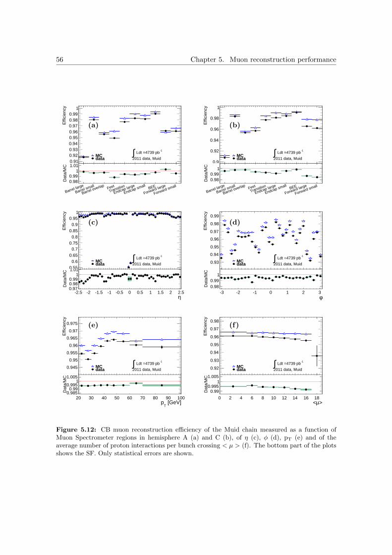
56 Chapter 5. Muon reconstruction performance
1 2 3 4 5 6 7 8 9 10
Effi
cien
cy
0.910.920.930.940.950.960.970.980.99
1
MC data
-1 Ldt =4739 pb∫
2011 data, Muid
Barrel large
Barrel small
Barrel overlapFeetTransition
Endcap large
Endcap smallBEE
Forward large
Forward small
Dat
a/M
C
0.980.99
11.01
(a)
1 2 3 4 5 6 7 8 9 10
Effi
cien
cy
0.9
0.92
0.94
0.96
0.98
1
MC data
-1 Ldt =4739 pb∫
2011 data, Muid
Barrel large
Barrel small
Barrel overlapFeetTransition
Endcap large
Endcap smallBEE
Forward large
Forward small
Dat
a/M
C
0.980.99
1
(b)
-2.5 -2 -1.5 -1 -0.5 0 0.5 1 1.5 2 2.5
Effi
cien
cy
0.550.6
0.650.7
0.750.8
0.850.9
0.951
MC data
-1 Ldt =4739 pb∫
2011 data, Muid
η-2.5 -2 -1.5 -1 -0.5 0 0.5 1 1.5 2 2.5
Dat
a/M
C
0.970.980.99
11.01
(c)
-3 -2 -1 0 1 2 3
Effi
cien
cy
0.93
0.94
0.95
0.96
0.97
0.98
0.99
MC data
-1 Ldt =4739 pb∫
2011 data, Muid
φ-3 -2 -1 0 1 2 3
Dat
a/M
C
0.980.99
1
(d)
20 30 40 50 60 70 80 90 100
Effi
cien
cy
0.945
0.95
0.955
0.96
0.965
0.97
0.975
MC data
-1 Ldt =4739 pb∫
2011 data, Muid
[GeV]T
p20 30 40 50 60 70 80 90 100
Dat
a/M
C
0.9850.99
0.9951
1.005
(e)
0 2 4 6 8 10 12 14 16 18
Effi
cien
cy
0.92
0.93
0.94
0.95
0.96
0.97
0.98
MC data
-1 Ldt =4739 pb∫
2011 data, Muid
>µ<0 2 4 6 8 10 12 14 16 18
Dat
a/M
C
0.990.995
11.005
(f)
Figure 5.12: CB muon reconstruction efficiency of the Muid chain measured as a function ofMuon Spectrometer regions in hemisphere A (a) and C (b), of η (c), φ (d), pT (e) and of theaverage number of proton interactions per bunch crossing < µ > (f). The bottom part of the plotsshows the SF. Only statistical errors are shown.

5.1. Measurement of the muon reconstruction efficiency 57
η-2.5 -2 -1.5 -1 -0.5 0 0.5 1 1.5 2 2.5
Effi
cien
cy
0.5
0.6
0.7
0.8
0.9
1
CBCB+ST
-1 Ldt =4739 pb∫2011 data, Staco
(a)
η-2.5 -2 -1.5 -1 -0.5 0 0.5 1 1.5 2 2.5
Effi
cien
cy
0.5
0.6
0.7
0.8
0.9
1
CBCB+ST
-1 Ldt =4739 pb∫2011 data, Muid
(b)
Figure 5.13: Efficiency of CB muons only (black circles) and of CB and ST muons (red triangles)reconstructed by the Staco (a) and the Muid (b) chains measured as a function of η for 2011 data.Only statistical errors are shown.
η-2.5 -2 -1.5 -1 -0.5 0 0.5 1 1.5 2 2.5
Effi
cien
cy
0.5
0.6
0.7
0.8
0.9
1
<2011>
periodB
periodD
periodE
periodF
periodG 2011 data, Muid
(a)
η-2.5 -2 -1.5 -1 -0.5 0 0.5 1 1.5 2 2.5
Effi
cien
cy
0.5
0.6
0.7
0.8
0.9
1
<2011>periodHperiodIperiodJperiodKperiodLperiodM 2011 data, Muid
(b)
Figure 5.14: CB muon reconstruction efficiency measured during the early (a) and late (b) 2011data taking periods for the Muid chain. The black points represent the average over the wholeyear. Only statistical errors are shown.
5.1.7 Systematic errors of the muon efficiency scale factors
The muon reconstruction efficiency scale factors are defined as a ratio, therefore most
systematic errors cancel. The reweighting of the zvtx and < µ > distributions (see Sec-
tion 5.1.4) ensures agreement in the description of the beam spot and of the pile-up
between data and Monte Carlo simulation. The dependence of the SF on the muon pT is
found to be negligible, as discussed in Section 5.1.6, therefore no correction of the muon
momentum resolution is taken into account for the simulated events. The main source
of systematic error is the background contribution to the measurement, which is entirely
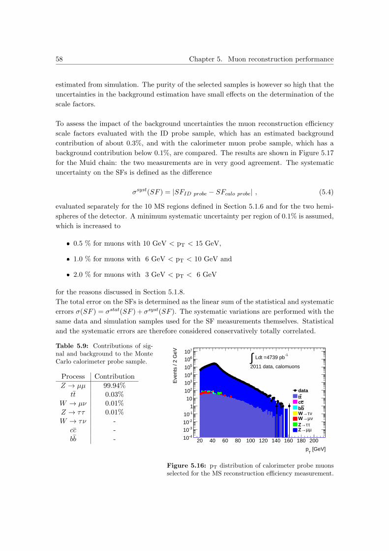
58 Chapter 5. Muon reconstruction performance
estimated from simulation. The purity of the selected samples is however so high that the
uncertainties in the background estimation have small effects on the determination of the
scale factors.
To assess the impact of the background uncertainties the muon reconstruction efficiency
scale factors evaluated with the ID probe sample, which has an estimated background
contribution of about 0.3%, and with the calorimeter muon probe sample, which has a
background contribution below 0.1%, are compared. The results are shown in Figure 5.17
for the Muid chain: the two measurements are in very good agreement. The systematic
uncertainty on the SFs is defined as the difference
σsyst(SF ) = |SFID probe − SFcalo probe| , (5.4)
evaluated separately for the 10 MS regions defined in Section 5.1.6 and for the two hemi-
spheres of the detector. A minimum systematic uncertainty per region of 0.1% is assumed,
which is increased to
0.5 % for muons with 10 GeV < pT < 15 GeV,
1.0 % for muons with 6 GeV < pT < 10 GeV and
2.0 % for muons with 3 GeV < pT < 6 GeV
for the reasons discussed in Section 5.1.8.
The total error on the SFs is determined as the linear sum of the statistical and systematic
errors σ(SF ) = σstat(SF ) + σsyst(SF ). The systematic variations are performed with the
same data and simulation samples used for the SF measurements themselves. Statistical
and the systematic errors are therefore considered conservatively totally correlated.
Table 5.9: Contributions of sig-nal and background to the MonteCarlo calorimeter probe sample.
Process Contribution
Z → µµ 99.94%tt 0.03%
W → µν 0.01%Z → ττ 0.01%W → τν -
cc -
bb -
[GeV]T
p
20 40 60 80 100 120 140 160 180 200
Eve
nts
/ 2 G
eV
-410
-310
-210
-110
1
10
210
310
410
510
610
710
datattccbb
ντ→Wνµ→W
ττ→Zµµ→Z
-1 Ldt =4739 pb∫
2011 data, calomuons
Figure 5.16: pT distribution of calorimeter probe muonsselected for the MS reconstruction efficiency measurement.

5.1. Measurement of the muon reconstruction efficiency 59
1 2 3 4 5 6 7 8 9 10
SF
0.94
0.95
0.96
0.97
0.98
0.99
1
1.01
1.02
ID probeCalo probe
-1 Ldt =4739 pb∫
2011 data, Muid
Barrel large
Barrel small
Barrel overlapFeetTransition
Endcap large
Endcap smallBEE
Forward large
Forward small
Rat
io
0.995
1
1.005
(a)
1 2 3 4 5 6 7 8 9 10
SF
0.94
0.95
0.96
0.97
0.98
0.99
1
1.01
ID probeCalo probe
-1 Ldt =4739 pb∫
2011 data, Muid
Barrel large
Barrel small
Barrel overlapFeetTransition
Endcap large
Endcap smallBEE
Forward large
Forward small
Rat
io
0.995
1
1.005
(b)
1 2 3 4 5 6 7 8 9 10
SF
0.95
0.96
0.97
0.98
0.99
1
1.01
1.02
ID probeCalo probe
-1 Ldt =4739 pb∫
2011 data, Muid
Barrel large
Barrel small
Barrel overlapFeetTransition
Endcap large
Endcap smallBEE
Forward large
Forward small
Rat
io
0.995
1
1.005
(c)
1 2 3 4 5 6 7 8 9 10
SF
0.95
0.96
0.97
0.98
0.99
1
1.01
1.02
ID probeCalo probe
-1 Ldt =4739 pb∫
2011 data, Muid
Barrel large
Barrel small
Barrel overlapFeetTransition
Endcap large
Endcap smallBEE
Forward large
Forward small
Rat
io
0.995
1
1.005
(d)
Figure 5.17: Comparison of the SF evaluated with ID probes (black circles) and with calorimeterprobes (red circles) for CB (a, b) and CB and ST muons (c, d) reconstructed by the Muid chainin side A (a, c) and C (b, d) of the spectrometer in 2011 data and simulation. The errors shownare statistical.
5.1.8 Muon reconstruction efficiency for low-pT muons
The measurement of the reconstruction efficiency and of the SF using the Tag-and-
Probe method in Z → µµ events is possible only above a certain pT threshold. Below
pT ≈ 20 GeV the background contribution is not negligible any more. The SF determi-
nation with ID probes has been extended down to pT = 15 GeV by using the calorimeter
probe method which is less affected by background. Both methods agree for pT > 20 GeV.
Below 15 GeV even the calorimeter probe samples starts to be affected by the background.
In order to evaluate the efficiencies for low-pT muons, a Tag-and-Probe analysis has been
performed on J/Ψ → µµ events [87] which confirmed the SF measurements in Z → µµ
events even for low-pT muons, although with large uncertainty. For this reason, the SFs
measured in Z → µµ events are used for the whole muon pT range but with increased sys-
tematic errors in the low pT region (see Sec .5.1.7) which are determined by a comparison
with the central value of the J/Ψ→ µµ measurement.

60 Chapter 5. Muon reconstruction performance
5.2 Measurement of the muon trigger and isolation effi-
ciency
In this section the efficiency of the muon isolation requirements applied in many analyses
to reduce the QCD multi-jet background contribution and of the muon trigger system
is studied using the Tag-and-Probe method. For the trigger efficiency measurement the
muon probes must be either combined or stand-alone muons. No isolation cut is applied
to the probes to avoid bias in the measurement, since the use of muon probes already
selects a very pure sample of Z → µµ events. The efficiency of a trigger requirement is
given by the fraction of probes matched with muons reconstructed by the event filter (EF)
within ∆R = 0.15. In the 2011 data set, the lowest threshold unprescaled muon triggers
are EF mu18 [88], requiring a single muon with pT > 18 GeV, for the early data taking
periods (B-I) at lower instantaneous luminosity, and EF mu18 medium [88] with the same
pT cut but tighter selection of the seeding first-level muons for the late periods (J-M). The
efficiency measurements shown in Fig. 5.18 have been performed for pT > 20 GeV, in the
plateau region of the trigger efficiency. In the endcap regions the trigger efficiency is about
85%. In the barrel region a stronger η dependency is found and the average efficiency is
about 75%.
The same method is used to measure the efficiency of the muon isolation requirements
The efficiency is defined as the fraction of muon probes which are isolated. The Z → µµ
selected sample consists mainly of isolated muons, but Z+ jets events also contribute. The
resulting efficiencies for a track isolation cut of∑∆R=0.3 ptracksT < 2.5 GeV and calorimeter
isolation cut of∑∆R=0.2EcaloT < 4 GeV are shown in Fig. 5.19. There is an excellent
agreement between data and simulations and no dependence on the muon pT and on the
pile-up conditions.
-2 -1.5 -1 -0.5 0 0.5 1 1.5 2
Effi
cien
cy
0
0.2
0.4
0.6
0.8
1
MC data -1
Ldt =1482 pb∫
2011 data, EF_mu18
η-2 -1.5 -1 -0.5 0 0.5 1 1.5 2
Dat
a/M
C
0.80.9
11.1
(a)
-2 -1.5 -1 -0.5 0 0.5 1 1.5 2
Effi
cien
cy
0
0.2
0.4
0.6
0.8
1
MC data -1
Ldt =3257 pb∫
2011 data, EF_mu18_medium
η-2 -1.5 -1 -0.5 0 0.5 1 1.5 2
Dat
a/M
C
0.80.9
11.1
(b)
Figure 5.18: Muon trigger efficiency measurement for 2011 data and simulation and SF forEF mu18 (a) and EF mu18 medium (b) trigger requirements. Statistical error only is shown.

5.2. Measurement of the muon trigger and isolation efficiency 61
-2.5 -2 -1.5 -1 -0.5 0 0.5 1 1.5 2 2.5
Effi
cien
cy
0.94
0.95
0.96
0.97
0.98
0.99
1
1.01
MC data
-1 Ldt =4739 pb∫
2011 data, Muid
η-2.5 -2 -1.5 -1 -0.5 0 0.5 1 1.5 2 2.5
Dat
a/M
C
0.99
1
1.01
Track isolation
-2.5 -2 -1.5 -1 -0.5 0 0.5 1 1.5 2 2.5
Effi
cien
cy
0.94
0.95
0.96
0.97
0.98
0.99
1
1.01
MC data
-1 Ldt =4739 pb∫
2011 data, Muid
η-2.5 -2 -1.5 -1 -0.5 0 0.5 1 1.5 2 2.5
Dat
a/M
C
0.99
1
1.01
Calorimeter isolation
20 40 60 80 100 120
Effi
cien
cy
0.94
0.95
0.96
0.97
0.98
0.99
1
1.01
MC data
-1 Ldt =4739 pb∫
2011 data, Muid
[GeV]T
p20 40 60 80 100 120
Dat
a/M
C
0.99
1
1.01
Track isolation
20 40 60 80 100 120
Effi
cien
cy
0.94
0.95
0.96
0.97
0.98
0.99
1
1.01
MC data
-1 Ldt =4739 pb∫
2011 data, Muid
[GeV]T
p20 40 60 80 100 120
Dat
a/M
C
0.99
1
1.01
Calorimeter isolation
0 2 4 6 8 10 12 14 16 18
Effi
cien
cy
0.94
0.95
0.96
0.97
0.98
0.99
1
1.01
MC data
-1 Ldt =4739 pb∫
2011 data, Muid
>µ<0 2 4 6 8 10 12 14 16 18
Dat
a/M
C
0.99
1
1.01
Track isolation
0 2 4 6 8 10 12 14 16 18
Effi
cien
cy
0.94
0.95
0.96
0.97
0.98
0.99
1
1.01
MC data
-1 Ldt =4739 pb∫
2011 data, Muid
>µ<0 2 4 6 8 10 12 14 16 18
Dat
a/M
C
0.99
1
1.01
Calorimeter isolation
Figure 5.19: Muon isolation efficiency measurement for 2011 data and simulation for a trackisolation cut of
∑∆R=0.3ptracksT < 2.5 GeV (left plots) and a calorimeter isolation cut of∑∆R=0.2
EcaloT < 4 GeV (right plots). Only statistical errors are shown.

62 Chapter 5. Muon reconstruction performance
5.3 Heavy flavour jet tagging efficiency
The Soft Muon Tagger (SMT) is an algorithm designed to discriminate heavy flavour
jets (c and b jets) from light-quark jets. The semileptonic decays of c and b hadrons are
exploited, in particular the muonic decays which provide a very clean signature. The ef-
ficiency reduction due to the semileptonic branching ratios of the heavy flavour hadrons,
of order 10%, is compensated by a high rejection factor for light-quark jets which rarely
contain muons, mostly non-prompt muons from pion and kaon decays which can be further
rejected with dedicated muon selection.
The SMT selects jets matched to a reconstructed muon within ∆R = 0.5, requiring
combined muons by the Staco chain (see Section 4.7) with pT>4 GeV, |d0| < 3 mm
and |z0 sin θ| < 3 mm,
ID track associated to the muon fulfilling the quality requirements of Table 5.3 and
a combination of the ID and the spectrometer track with χ2match < 3.2 (see Sec-
tion 4.7).
The use of combined muons ensures an strong fake rejection at high muon efficiency.
The track quality cuts of Table 5.3 and the cuts on the impact parameter of the muon
track reduce the contamination from non-prompt muon. The χ2match cut also reduces the
non-prompt muons contributions since pions and kaons have rather long lifetimes and on
average decay after flight distance of the order of a metre in the ID leading to a bias in
the ID track and to a higher χ2match value. The mistag rate of the tagger, i.e. the fraction
of light-quark jets which are wrongly tagged as heavy-flavour jets, has been measured in a
data sample on QCD multi-jet events to be 0.2%-0.5% depending on the η and pT of the jet.
The efficiency of the soft muon tagger measured in Monte Carlo simulation is corrected
with data-driven techniques to match the efficiency in the data. The tagging efficiency de-
pends on the branching ratio of the semimuonic heavy-flavour decays, on their kinematics
and on the final state selection applied. An example of such effects is given in Section 7.9.3
in the context of the W+ c-jets cross section measurement. However, the efficiency of the
muon selection applied by the SMT only depends on the muon kinematics and can thus
be measured using the Tag-and-Probe method as described below.
The measurement of the efficiency of the muon selection criteria applied by the SMT
has been performed with J/Ψ → µµ and Z → µµ events. In this section the latter are
discussed. The tag definition of Section 5.1.4 is used, and CB muons with pT > 10 GeV
are used as muon probes. The efficiency is the fraction of muon probes satisfying the SMT
requirements. The χ2match distribution of the selected muon probes is shown in Fig. 5.20
The results are shown in Fig. 5.21. The SF decrease with increasing pT due to the ideal
MS alignment which is assumed as a standard in the Monte Carlo simulation. In the

5.3. Heavy flavour jet tagging efficiency 63
region η > 2, corresponding to the detector region in which Cathode Strip Chambers are
used in the hemisphere A of the muon spectrometer, a strong drop of the efficiency in the
simulation is visible, which is due to an error in the simulation of the detector response
resulting in a χ2match distribution with much bigger tails than in the corresponding region
η < -2 of the hemisphere C, as shown in Fig. 5.22f. Fig. 5.23 shows the comparison of the
efficiencies and SF for simulations with ideal alignment and with realistic misalignment. In
the latter case, the pT dependence of the SF is significantly reduced. The pT dependence
is not too relevant for the practical applications of the SMT: muon resulting from b and
c hadrons decays have low transverse momentum, usually below 30 GeV, a region where
the pT dependence is less significant.
The possible bias introduced by the efficiency measurement performed in a Z → µµ sam-
ple, with mostly isolated muons, while the SMT selection criteria are applied to muons
inside jets has been studied in a sample of probe muons selected without the usual isolation
cut adopted for the Tag-and-Probe method. It is shown in Fig. 5.24 that the efficiency
measurement does not depend significantly on the isolation of the muons.
The systematic error of the SF in this case cannot be determined by changing the probe def-
inition as it was done for the reconstruction efficiency measurement. To study the impact of
uncertainties in the background contribution to the sample of muon probes the cut on tag-
and-probe invariant mass has been varied from the nominal cut of |mµµ − mZ | < 10 GeV
to 7.5 GeV and 15 GeV. Similarly the probe track isolation cut has been varied from∑∆R=0.4 ptracksTpT
muon < 0.2 to 0.1 and 0.3.
The total systematic error is determined as the quadratic sum of both contributions (see
Fig. 5.25) and found to be small. The total error on the SF is the linear sum of the
statistical and systematic error (see Section 5.1.6).
The SMT SFs used for the W+ c-jet cross section measurement described in Chapter 7
are determined as a function of η and pT in the low-pT region, where the measurement
has been performed in J/Ψ→ µµ events, and as a function of pT and MS region for muon
pT>12 GeV, where the measurement has been performed with Z → µµ events.

64 Chapter 5. Muon reconstruction performance
/NDOFmatch2χ
0 1 2 3 4 5 6 7 8 9 10
Nor
mal
ised
to u
nity
0
0.02
0.04
0.06
0.08
0.1
0.12
0.14
data
MC
-1 Ldt =4739 pb∫
2011 data, Staco
Figure 5.20: χ2match distribution of muon probes from Z → µµ events in 2011 data and simulation
normalised to unity.
-2.5 -2 -1.5 -1 -0.5 0 0.5 1 1.5 2 2.5
Effi
cien
cy
0.550.6
0.650.7
0.750.8
0.850.9
0.951
MC data
-1 Ldt =4739 pb∫
2011 data, Staco
η-2.5 -2 -1.5 -1 -0.5 0 0.5 1 1.5 2 2.5
Dat
a/M
C
0.951
1.05
(a)
20 40 60 80 100 120 140 160 180 200
Effi
cien
cy
0.7
0.75
0.8
0.85
0.9
0.95
1
MC data
-1 Ldt =4739 pb∫
2011 data, Staco
[GeV]T
p20 40 60 80 100 120 140 160 180 200
Dat
a/M
C
0.80.9
1
(b)
Figure 5.21: SMT muon selection efficiency and scale factor as a function of η (a) and pT (b) for2011 data and simulation.

5.3. Heavy flavour jet tagging efficiency 65
/NDOFmatch2χ
0 1 2 3 4 5 6 7 8 9 10
Nor
mal
ised
to u
nity
0
0.02
0.04
0.06
0.08
0.1
0.12
0.14
0.16
Barrel Large A dataBarrel Large A MCBarrel Large C dataBarrel Large C MC
-1 Ldt =4739 pb∫
2011 data, Staco
(a) Large barrel region
/NDOFmatch2χ
0 1 2 3 4 5 6 7 8 9 10
Nor
mal
ised
to u
nity
0
0.02
0.04
0.06
0.08
0.1
0.12
0.14
Barrel Small A dataBarrel Small A MCBarrel Small C dataBarrel Small C MC
-1 Ldt =4739 pb∫
2011 data, Staco
(b) Small barrel region
/NDOFmatch2χ
0 1 2 3 4 5 6 7 8 9 10
Nor
mal
ised
to u
nity
0
0.02
0.04
0.06
0.08
0.1
0.12
0.14
Endcap Large A dataEndcap Large A MCEndcap Large C dataEndcap Large C MC
-1 Ldt =4739 pb∫
2011 data, Staco
(c) Large endcap region
/NDOFmatch2χ
0 1 2 3 4 5 6 7 8 9 10
Nor
mal
ised
to u
nity
0
0.02
0.04
0.06
0.08
0.1
0.12
0.14
Endcap Small A dataEndcap Small A MCEndcap Small C dataEndcap Small C MC
-1 Ldt =4739 pb∫
2011 data, Staco
(d) Small endcap region
/NDOFmatch2χ
0 1 2 3 4 5 6 7 8 9 10
Nor
mal
ised
to u
nity
0
0.02
0.04
0.06
0.08
0.1
0.12
CSC Large A dataCSC Large A MCCSC Large C dataCSC Large C MC
-1 Ldt =4739 pb∫
2011 data, Staco
(e) Large CSC region
/NDOFmatch2χ
0 1 2 3 4 5 6 7 8 9 10
Nor
mal
ised
to u
nity
0
0.02
0.04
0.06
0.08
0.1
0.12
0.14
CSC Small A dataCSC Small A MCCSC Small C dataCSC Small C MC
-1 Ldt =4739 pb∫
2011 data, Staco
(f) Small CSC region
Figure 5.22: χ2match distributions for muon probes with 10 GeV < pT < 30 GeV normalised
to unity area evaluated in 2011 data and simulations for different MS regions. Regions in side A(η > 0) are drawn in black, regions in side C (η < 0) in red (see Section 5.1.1).

66 Chapter 5. Muon reconstruction performance
10 20 30 40 50 60 70 80 90 100
Effic
ien
cy
0.82
0.84
0.86
0.88
0.9
0.92
0.94
0.96
0.98
1
tagandprobeµµ→Z
2011 data, chain 1 MC data
[GeV]T
p
10 20 30 40 50 60 70 80 90 100
SF
0.95
1
∫Ldt = 4739 pb−1
(a)
10 20 30 40 50 60 70 80 90 100
Effic
ien
cy
0.82
0.84
0.86
0.88
0.9
0.92
0.94
0.96
0.98
1
tagandprobeµµ→Z
2011 data, chain 1 MC data
[GeV]T
p
10 20 30 40 50 60 70 80 90 100
SF
0.95
1
∫Ldt = 4739 pb−1
(b)
Figure 5.23: SMT muon selection efficiency in 2011 data and simulation and the SF as a functionof pT for simulation with ideal MS alignment (a) and with realistic misalignment (b).
0 5 10 15 20
Effi
cien
cy
0.8
0.85
0.9
0.95
1
MC data
-1 Ldt =4739 pb∫
2011 data, Staco
Calo Iso [GeV]0 5 10 15 20
Dat
a/M
C
0.920.940.960.98
1
(a)
0 5 10 15 20
Effi
cien
cy
0.8
0.85
0.9
0.95
1
MC data
-1 Ldt =4739 pb∫
2011 data, Staco
Calo Iso [GeV]0 5 10 15 20
Dat
a/M
C
0.920.940.960.98
1
(b)
Figure 5.24: SMT muon selection efficiency in 2011 data and simulation and SF as a function ofthe calorimeter isolation cut on the probe in side A (a) and C (b) of the muon spectrometer.

5.3. Heavy flavour jet tagging efficiency 67
1 2 3 4 5 6 7 8 9 10
SF
0.9
1
1.1
1.2
1.3
1.4
nominal cutinvloose M
-1 Ldt =4739 pb∫
2011 data, Staco
Barrel large
Barrel small
Barrel overlapFeetTransition
Endcap large
Endcap smallBEE
Forward large
Forward small
Rat
io
0.995
1
1.005
(a)
1 2 3 4 5 6 7 8 9 10
SF
0.88
0.9
0.92
0.94
0.96
0.98
1
nominal cutinvloose M
-1 Ldt =4739 pb∫
2011 data, Staco
Barrel large
Barrel small
Barrel overlapFeetTransition
Endcap large
Endcap smallBEE
Forward large
Forward small
Rat
io
0.9951
1.005
(b)
1 2 3 4 5 6 7 8 9 10
SF
0.9
1
1.1
1.2
1.3
1.4
nominal cut
invtight M
-1 Ldt =4739 pb∫
2011 data, Staco
Barrel large
Barrel small
Barrel overlapFeetTransition
Endcap large
Endcap smallBEE
Forward large
Forward small
Rat
io
0.995
1
1.005
(c)
1 2 3 4 5 6 7 8 9 10
SF
0.88
0.9
0.92
0.94
0.96
0.98
1
nominal cut
invtight M
-1 Ldt =4739 pb∫
2011 data, Staco
Barrel large
Barrel small
Barrel overlapFeetTransition
Endcap large
Endcap smallBEE
Forward large
Forward small
Rat
io
0.9951
1.005
(d)
1 2 3 4 5 6 7 8 9 10
SF
0.9
1
1.1
1.2
1.3
1.4
nominalloose isolation cut
-1 Ldt =4739 pb∫
2011 data, Staco
Barrel large
Barrel small
Barrel overlapFeetTransition
Endcap large
Endcap smallBEE
Forward large
Forward small
Rat
io
0.995
1
1.005
(e)
1 2 3 4 5 6 7 8 9 10
SF
0.88
0.9
0.92
0.94
0.96
0.98
1
nominalloose isolation cut
-1 Ldt =4739 pb∫
2011 data, Staco
Barrel large
Barrel small
Barrel overlapFeetTransition
Endcap large
Endcap smallBEE
Forward large
Forward small
Rat
io
0.9951
1.005
(f)
1 2 3 4 5 6 7 8 9 10
SF
0.9
1
1.1
1.2
1.3
1.4
nominaltight isolation cut
-1 Ldt =4739 pb∫
2011 data, Staco
Barrel large
Barrel small
Barrel overlapFeetTransition
Endcap large
Endcap smallBEE
Forward large
Forward small
Rat
io
0.995
1
1.005
(g)
1 2 3 4 5 6 7 8 9 10
SF
0.88
0.9
0.92
0.94
0.96
0.98
1
nominaltight isolation cut
-1 Ldt =4739 pb∫
2011 data, Staco
Barrel large
Barrel small
Barrel overlapFeetTransition
Endcap large
Endcap smallBEE
Forward large
Forward small
Rat
io
0.9951
1.005
(h)
Figure 5.25: Systematic errors of the SMT muon selection efficiency SF determined as a functionof the MS region for side A (left plots) and C (right plots) of the spectrometer by varying thetag and probe invariant mass cut applied in the selection of the sample to looser (a,b) and tighter(c,d) values and varying the isolation cut on the probe to looser (e,f) and tighter (g,h) values.The SF determined with the nominal (black circles) and modified (red triangles) cuts are shown.The bottom part of the plots shows the ratio between the two determinations, the green bandrepresents the statistical error on the ratio.

68 Chapter 5. Muon reconstruction performance
5.4 Conclusion
The performance of the ATLAS Inner Detector and Muon Spectrometer have been studied
in data collected in 2011 and in Monte Carlo simulation using the Tag-and-Probe method
in Z → µµ events.
The Inner Detector reconstruction efficiency for muon tracks is found to be nearly 1 in
the data and simulation. The inefficiency introduced for muon ID tracks by the quality
criteria applied to reject the contribution of non-prompt muons is measured in data to
be about 1.6%, slightly higher than the expectation in simulations of 1.4%. The muon
reconstruction efficiency for the combined reconstruction of ID and MS tracks is found to
be higher than 95% in data, in good agreement with the simulations. Corrections factors
of the order of 1% have been derived for the Monte Carlo events. No dependence is found
on the pT of the muon and on the pile-up conditions for the muon reconstruction. The
systematic uncertainties of the correction factors for the simulations have been assessed
to be at 0.1% level.
The efficiency of the cuts on muon isolation variables applied in physics analyses to reject
mainly the QCD multi-jet background is found to be perfectly described by simulation.
The trigger efficiency is found to be about 80% for the even filter algorithms used for the
2011 data set.
The efficiency of the muon selection criteria applied by the Soft Muon Tagger which iden-
tifies heavy-flavour jets is found to about 90% in data. In this case larger corrections scale
factors are needed for Monte Carlo events since no misalignment is considered by default
in the simulations. These corrections are anyway below 5% in the low pT region of the
semimuonic decays of heavy-flavour hadrons.
In conclusion, excellent performance are found for the ATLAS muon reconstruction and
identification in the data set collected during 2011 in agreement with the expectations,
a result confirmed by the measurements performed for the 2012 data set reported in
Appendix B.

Chapter 6
Measurement of the W+ b-jet
production cross section
The production of W bosons associated with jets (W+ jets) is a process predicted by the
Standard Model (see Section 2.2). In second order perturbation theory, bottom quark-
antiquark pairs are produced in association with a W boson according to the Feynman
diagrams shown in Figure 6.1. Final states with a single b quark are suppressed because
of the small values of the CKM matrix elements Vub and Vcb.
The study of W+ b-jets production is an important test of perturbative QCD predictions.
A measurement of the W+ b-jets production cross section performed by the CDF experi-
ment [89] shows an excess over theoretical predictions, although with large uncertainties.
W+ b-jets events are also an important background for the search for H → bb decays
in the process pp → WH + X → Wbb + X, for single top quark and top quark tt pair
production, and for processes predicted by theories beyond the Standard Model.
In this chapter, a measurement of the W+ b-jets production cross section with the ATLAS
detector [1], which is the result of the efforts of a small analysis team, is described. The
main contributions of this work are the signal event selection including measurement of
the selection efficiency and the cross section determination with the assessment of the
systematic uncertainties.
6.1 Data samples used for the analysis
The study of W+ b-jets production presented here uses an integrated luminosity of
35.5 pb−1 of proton-proton collisions data at√
s=7 TeV, collected by the ATLAS de-
tector during 2010. Only W → eν and W → µν decays are considered in the analysis.
The background processes taken into account for the measurement are listed in Table 6.1.
W+ b-jets production via t → W + b decays is not included in the signal definition and
69

70 Chapter 6. Measurement of the W+ b-jet production cross section
(a) LO diagram (b) NLO diagram
Figure 6.1: Feynman diagrams for W+ b-jets production in proton-proton collisions: (a) leadingorder (LO) and (b) next-to-leading order (NLO).
therefore taken into account as a background. The contributions of Z+ jets events and
of diboson and single-top productions are small and therefore estimated by Monte Carlo
simulation. The largest background contributions are due to tt and W+ jets events which
are determined by data-driven techniques using Monte Carlo simulations for the shapes
of discriminating variables used for event selection. The QCD multi-jet background is
entirely estimated from data.
W+ jets processes are generated using Alpgen [47], interfaced with Herwig [45] for the
parton shower and with Jimmy [53] for the underlying event simulation. The production
processes W+0-5 partons (W+ light-jets), W + c+0-4 partons, W + cc+0-3 partons and
W + bb+0-3 partons are separately generated by Alpgen: the matrix element is therefore
calculated for each process with a fixed number of outgoing partons, and the resulting 19
simulated sample are combined to completely describe W+ jets production. The proce-
dures for the removal of overlap between the samples are described in Section 6.1.1.
Alpgen+Herwig samples are used to simulate the Z+ jets background. The tt back-
ground sample was generated using MC@NLO [49]. The single-top background is simu-
lated with AcerMC [51] for the t-channel and for the Wt-channel, while the s-channel is
simulated with MC@NLO. Herwig has been used for the simulation of the WW , WZ,
ZZ diboson production. The different Monte Carlo generators have been introduced in
Section 2.3.
6.1.1 Overlap removal for the Alpgen W+ jets samples
The Alpgen W+ jets samples are generated with a given fixed number of hard par-
tons. Partons are considered hard if they have pT > 15 GeV. Hard partons must also be
separated by ∆R > 0.7. For the analysis, a maximum of five hard partons is considered.

6.1. Data samples used for the analysis 71
Table 6.1: Monte Carlo event signal and background samples used for the W+ b-jets cross sectionmeasurement. The total cross section of the four W+ jets samples is normalised to the NNLO Winclusive production cross section calculated in [33].
Physics process Generator σ · BR [nb]
W→ lν +bb Alpgen[47]W→ lν +jets Alpgen[47]W→ lν +cc Alpgen[47]W→ lν +c Alpgen[47]
Total W→ lν + jets 10.46 NNLO [33]
tt MC@NLO[49] 89.7 approx. NNLO [85]QCD multi-jet - contribution estimated in datasingle-top (s-channel) MC@NLO[49] 4.3×10⁻⁴ NLO [40]single-top (t-channel) AcerMC[51] 6.34×10⁻³ NLO [40]single-top (Wt) AcerMC[51] 13.1×10⁻³ NLO [40]Z → `` + jets (m`` > 40 GeV) Alpgen[47] 1.07 NNLO [33]WW Herwig [45] 44.9×10⁻³ NLO [40]WZ Herwig [45] 18.5×10⁻³ NLO [40]ZZ Herwig [45] 5.7×10⁻³ NLO [40]
The Alpgen generator describes the hard scattering process (see Section 2.3) while the
evolution of the partons via soft QCD interactions, i.e. the parton shower (PS), is sim-
ulated with a second generator, Herwig in this case. The PS algorithm can generate
jets at small relative angle. Some collinear jets are also produced according to the matrix
elements (ME) of the Alpgen generator. In order to avoid double counting of these jets,
an overlap removal procedure is applied using the MLM matching scheme[90] for the in-
terface of the ME and PS algorithms. After the showering performed by Herwig, jets are
formed from the generated particles using a clustering algorithm. These jets are required
to have pT > 20 GeV. The hard parton with the highest pT is associated to the jet closets
within ∆R <0.7 which is removed from the list of jets. The procedure is repeated for the
remaining partons. Events are kept only if each hard parton is matched with a jet and
if there are no unmatched jets. Events with unmatched jets are kept only in the sample
with the highest multiplicity of hard partons.
Alpgen samples with heavy flavour quark production at ME level are also produced sep-
arately. The Alpgen samples used are W (+ 0-5 partons), W + cc (+ 0-3 partons),
W + bb (+ 0-3 partons), W + c (+ 0-4 partons). A second kind of overlap must be taken
into account when the samples for the different quark flavours are combined. For example,
a final state with W , u quark and a bb pair can arise either from the W + bb + 1-parton
Alpgen sample or from the W+1-parton sample with a bb pair produced by the PS al-
gorithm. The solution applied relies on the assumption that the ME describes bb final
states with a large angle between the two b quarks, while the PS algorithm describe the

72 Chapter 6. Measurement of the W+ b-jet production cross section
final states with more collinear b quarks. Therefore events containing a bb pair are kept in
the W+ light-jets sample, where they only originate from PS, only if the angle between
the two b quarks is ∆R <0.4. Similarly, in the W + bb sample events are kept only if the
b quarks are separated by ∆R >0.4.
For the c quarks, the situation is slightly different. While in the W+ light-jets sample
there are no b quarks in the initial state partons at ME level, massless c quarks are taken
into account1. When combining the samples all events with c quarks at ME level are
therefore removed from the W+ light-jets sample, as this process is completely described
by the dedicated W + c sample. The same overlap removal procedure as for bb pairs is
applied also to cc pairs.
This second overlap removal procedure is referred to as Heavy Flavour Overlap Removal
(HFOR).
6.2 Event selection
The event selection criteria for the cross section measurement are summarized in Table 6.2.
6.2.1 Preselection
Events used for the analysis were collected with the ATLAS detector subsystems fully
operational. The primary vertex of the event is required to be associated to at least 3 ID
tracks in order to reject cosmic muon events which have a vertex with two associated tracks.
In the Monte Carlo simulations, two general corrections similar to the ones described in
Section 5.1.4 are applied. Events are reweighted according to the pile-up conditions and
the longitudinal size of the beam spot observed in the data. The first correction is per-
formed by weighting with the ratio of the numbers of reconstructed vertices with at least
3 associated tracks in data and Monte Carlo events (which is a measure of the pile-up
level). The second correction is performed by reweighting such that the distribution of
the z coordinate of the primary vertex in simulations matches the one in the data.
6.2.2 Trigger requirements
The least stringent unprescaled trigger requirements are used. For the electron channel
this is EF e15 medium trigger which requires an electron with pT > 15 GeV. For the
1This modellization is known as 4-flavours numbering scheme (4FNS). u, d, s, c quarks (and correspond-ing antiparticles) are considered to be present in the proton with their own PDF, while b and t quarks (andcorresponding antiparticles) are produced only via gluon splitting. In the 5-flavours numbering scheme(5FNS) b quarks have their own PDF and are considered also in the initial state.

6.2. Event selection 73
muon channel, three different algorithms have been used in different data taking periods
in 2010:
EF MU10 MSonly, requiring a muon track reconstructed in the MS with pT > 10 GeV,
in the early periods,
EF MU13, requiring a combined muon track with pT > 13 GeV for intermediate
luminosities in the middle period and
EF MU13 tight, requiring a combined muon track with pT > 13 GeV with tighter
cuts on the pT of the seeding muon selected at the first trigger level (see Sec-
tion 3.2.6.1), for the late data taking period with the highest instantaneous lu-
minosities.
The lepton candidates selected by the trigger algorithms are required by the analysis se-
lection to match within ∆R <0.15 the leptons reconstructed offline, to ensure that no bias
is introduced by the trigger.
6.2.3 Lepton selection
The pT cut of 20 GeV applied to the reconstructed electrons and muons ensures that
the trigger algorithms are working in the efficiency plateau region. An η cut is applied,
corresponding to the detector acceptance for the electrons and to the acceptance of the
trigger chambers for the muons. Electrons in the transition region between barrel and
endcap, corresponding to 1.37< |η| <1.52, are removed because of gaps in the calorimeter
coverage in this region. Electrons are selected using the tight identification criteria (see
Section 4.3). Combined (CB) muon tracks are used (see Section 4.7) applying the qual-
ity cuts of Table 5.3 on the ID track associated to the muon. Corrections for the muon
reconstruction and identification efficiencies, for the electron energy resolution and for
the muon momentum resolution are applied to the simulated events to match the perfor-
mance measured in the data (see [71] for the electron and [91, 92] for the muon corrections).
In order to reject the QCD multi-jet background, the leptons are required to be isolated.
In the electron channel, a combination of track and calorimeter isolation requirements
with an expected signal efficiency of 95% is applied (see [69]). An η-dependent correction
is applied to the isolation efficiency in simulations to match the performance measured in
data [71]. Muons are required to have an angular distance with respect to the nearest jet
of ∆R(µ, jet) >0.4. A 4 GeV cut on the track and calorimeter isolation variables, in both
cases for a cone radius ∆R = 0.3, is also applied. More details on the isolation criteria
are given in Section 4.8.
For the electron channel, events with exactly one electron and no muons are selected. For
the muon channel, exactly one muon and no electrons are required. The dilepton veto

74 Chapter 6. Measurement of the W+ b-jet production cross section
Table 6.2: Events selection criteria used for the W+ b-jets cross section measurement
Cut W → eν channel W → µν channel
Preselection
Data taking conditions All sub-detectors and systems in optimal working conditionsPrimary vertex nPVtracks ≥ 3
Trigger algorithm EF e15 mediumEF MU10 MSonly (early data)
EF MU13 (middle period)EF MU13 tight (late data)
Trigger matching offline selected lepton within ∆R < 0.15 to trigger object
W selection
Lepton identification tight (see Section 4.3)CB muon (see Section 4.7),
quality cuts in Table 5.3
Kinematic cutsET >20 GeV pT > 20 GeV|η| <2.47 |η| <2.4
|η| <1.37 or |η| >1.52
Lepton isolation iso95 (see text and [69])∆R(µ, jet) > 0.4∑∆R=0.3 ptracksT < 4 GeV∑∆R=0.3EcaloT < 4 GeV
Selected leptons 1 electron, no muons 1 muon, no electrons
Missing energy EmissT > 25 GeV
W transverse mass mWT > 40 GeV
Jet selection
Kinematic cutspT > 25 GeV|y| < 2.1
Quality cuts Loose criteria (see Section 4.4 and [73])Pile-up cleaning Jet vertex fraction JVF > 0.75 (see text)Jets multiplicity njets=1 or 2
b-jet selection
SV0 b-tagger L/σ(L) > 5.85b-jet multiplicity nSV 0
tagged jets=1
rejects Z+ jets and tt backgrounds.
6.2.4 W boson selection
The events are required to have a transverse momentum imbalance of EmissT > 25 GeV
to account for the presence of a neutrino in the W decay. The EmissT reconstruction is
described in Section 4.6. In the Monte Carlo simulations, all corrections applied to the
momenta of the different reconstructed objects are propagated to the EmissT .
The transverse mass of the W is determined from the momentum of the selected lepton
and EmissT according to:

6.3. Background estimation 75
mWT =
√2pT
leppTν(1− cos(φlep − φν)) . (6.1)
A mWT > 40 GeV cut is applied.
6.2.5 Jet selection and b-jet tagging
Jets are reconstructed using the anti-kT algorithm with a distance parameter R = 0.4.
They are reconstructed from energy clusters in the calorimeters at the EM scale and are
then recalibrated to the hadronic scale (see Section 4.4). The jets are required to have
pT > 25 GeV and |y| < 2.1, in the fiducial region of the b-tagging algorithm used in the
measurement. The loose quality cuts [73] are applied to the jets. In order to reject jets
from pile-up interactions a cut of JVF > 0.75 is applied on the jet vertex fraction. This
variable is defined as the fraction of the sum of transverse momenta of the tracks in the
jet which belongs to tracks associated to the primary vertex. Events are classified in two
categories with exactly one and exactly two selected jets respectively.
In the one-jet category the jet is required to be tagged as a b-jet by the SV0 tagging algo-
rithm [77] described in Section 4.4.4.1. The SV0 tagger is used at a working point which
ensures a selection efficiency for b-jets of about 35%. Simulated events are reweighted to
reproduce the SV0 performance measured in data. In the two-jets category only one of
the jets is required to be tagged as a b-jet, while events with both jets tagged as b-jets
are vetoed: the fraction of W + bb events in which two true b-jets are reconstructed and
tagged is about 2%, due to detector acceptance effects, the kinematic cuts applied and
the b-tagging efficiency and because the two b quarks may not be resolved in separated
jets. Furthermore, the two-jets category with both jets tagged as a b-jets has a very high
background contribution from tt production.
The efficiency of the b-jet tagging and the rate of c and light-jets passing the SV0 selection
are corrected in the simulations to match the efficiency and mistag rate measured in
data [78].
6.3 Background estimation
The contributions of W + cc, W + c and W+ light-jets, tt and QCD multi-jet production
processes are estimated with data-driven techniques explained in this section. All other
backgrounds are estimated from Monte Carlo simulations.
6.3.1 The W+ jets background
The b-jet tagging requirement reduces the background due to the production of a W boson
in association with charm or with light-quark jets, but the cross sections of these processes

76 Chapter 6. Measurement of the W+ b-jet production cross section
are much higher than the signal cross section leading to a non-negligible contribution of
these backgrounds. Final states including c quarks are most problematic, since the mistag
rate of the b-tagger is much higher for c-jets than for light-jets due to the relatively long
lifetime of charm hadrons.
In order to determine the contributions of these processes the higher mass of the b-hadrons
compared to others is exploited. The invariant mass mSV of the tracks emerging from a
secondary vertex reconstructed inside a b-jet serves as discriminating variable.
The fractions of events with b-jets, c-jets and light-jets in the selected data sample are
determined by a fit of a linear superposition of the mSV distributions for all contributing
processes to the mSV distribution measured in data. In this fit, the fractions of W+ b-jets,
W+ c-jets and W+ light-jets events are used as free parameters, while the distributions
for all other background processes are normalised to the predictions obtained as described
below. The mSV template shapes for W+ b-jets, W+ c-jets and W+ light-jets events are
determined from Monte Carlo simulations. The mSV distribution for tt events is taken
from simulation and normalised to the number of tt events passing the selection, which is
estimated from data as described in Section 6.3.2. The mSV distribution for QCD multi-
jet events and its normalisation are determined using a data control region as discussed
in Section 6.3.3.
The results of the fit in each of the two event categories in the two lepton channels are
shown in Fig. 6.2. The results of the fit to the data agree with the simulations, especially
in bins dominated by background. This means that the modelling of the background
processes is correct. The numerical results are given in Table 6.3.
6.3.2 The tt background
tt production contributes to the background because of the t→W + b decays, which have
a BR of almost 100%. The resulting final states have W bosons and b-jets with similar
properties as for the signal one but with a much higher average number of jets.
The tt contribution is first determined from a control data set defined by events with at
least four jets including one or more b-tagged jets. This control data sample is domi-
nated by tt events and has contributions from W+ b-jets and QCD multi-jet events. A
fit of a superposition of the mSV templates for tt, W+ b-jets and multi-jet events is used
to determine the number of tt events in the control sample. The mSV templates for tt
and for W+ b-jets events are determined by Monte Carlo simulations while the shape
for QCD multi-jet events is determined in a control data sample defined in Section 6.3.3.
The normalisation of the W+ b-jets contribution is fixed to the Monte Carlo prediction,
with an assigned uncertainty of 100%. In the electron channel, the QCD multi-jet mSV
template is normalised with the same data-driven technique as described in Section 6.3.3.
The normalisation of the tt template is therefore the only free parameter of the mSV fit

6.3. Background estimation 77
(a) (b)
(c) (d)
Figure 6.2: mSV distributions for the b-tagged jets in data and Monte Carlo simulations in the1-jet (a and c) and 2-jet (b and d) event category for the electron (a and b) and the muon channels(c and d) [1]. The Monte Carlo distributions for W+ b-jet(s), W+ c-jet(s) and W+ light-jetsevents are normalised to their fitted contribution in data. The normalisation of the tt and theQCD multi-jet background are determined with data driven techniques. Other backgrounds arefrom Monte Carlo simulations.
in the control region. In the muon channel, the fit of the mSV distribution is performed
simultaneously with a fit to the track-based muon isolation variable which fixes the nor-
malisation of the QCD multi-jet contribution.
The number of tt background events in the selected W+ b-jets data sample is determined
as the number of tt events measured in the control sample multiplied by the ratio of tt
events in signal and control regions predicted by Monte Carlo simulation. The advantage
of this approach is that the the uncertainty in the b-tagging efficiency and mistag rate,
which are the biggest systematic errors for the measurement, mostly cancels in the ratio.
The main source of uncertainty for the tt background estimation is the error in the jet
energy scale. Other systematic uncertainties are negligible. The error on the tt background
78 Chapter 6. Measurement of the W+ b-jet production cross section
normalisation is 20-25% in the 1-jet and 2-jet categories for both lepton channels. The tt
background prediction is shown in Table 6.3.
6.3.3 The QCD multi-jet background
QCD multi-jet productions contribute to the background mostly due to the limited detec-
tor resolution and to misreconstructed events. In the electron channel, jets and photons
may be misidentified as electrons. Electrons and muons from heavy-flavour hadrons de-
cays may wrongly be classified as isolated. Non-prompt muons from pion and kaon decays
may be wrongly attributed to W boson decays. QCD multi-jet cross sections have large
theoretical uncertainties and these processes are not modelled well enough and with suffi-
cient statistics by Monte Carlo simulations after the very strong rejection by the analysis
cuts. But even with high rejection, QCD multi-jet final states contribute significantly be-
cause of their high cross sections. The QCD multi-jet background is therefore determined
exclusively by using data-driven techniques. The results are presented in Table 6.3.
6.3.3.1 Electron channel
In the electron channel, the data EmissT distribution is fitted in the 0-100 GeV range using
two templates, one for QCD multi-jet events and the other one for the signal and all the
other backgrounds. The normalisation of the multi-jet background is determined by the fit.
The multi-jet EmissT template is obtained from a data control sample dominated by multi-
jet events and obtained applying a modified event selection with no EmissT cut and with an
electron selection which requires passing the loose electron identification (see Section 4.3)
but failing medium and tight requirements. An electron trigger condition based on loose
electron identification has been used to avoid bias. The multi-jet EmissT distribution has
been studied in Monte Carlo simulations and shows no distortion due to the inverted elec-
tron identification compared to the nominal one. The EmissT template for signal and all
other backgrounds is determined from Monte Carlo simulations. The EmissT distribution
in the signal region (without any cut on the EmissT ) is shown in Fig. 6.3 with the multi-jet
component from the fit. The low EmissT region with significant contribution from multi-jet
events is well described.
The multi-jet background normalisation has a 50% uncertainty due to the statistical error
of the EmissT data distribution and of the templates, which is the dominant error. System-
atic studies have been performed by changing the definition of the control region used to
define the multi-jet EmissT template.
6.3.3.2 Muon channel
In the muon channel, the multi-jet background is estimated using the so-called matrix
method described in [93]. Two data samples with loose and tight muon selection are
defined, where the second one is a subset of the first, differing only by the muon selection

6.3. Background estimation 79
Figure 6.3: EmissT distribution in the W+ b-jets signal region for the electron channel without
EmissT cut [1]. The multi-jet contribution is normalised to the data-driven prediction while all other
contributions are from to Monte Carlo simulations.
used. The tight selection is the nominal selection while for the loose selection the muon
isolation requirements are removed, requiring only that the selected muon is separated
from selected jets by ∆R >0.4. Both samples contains contributions of fake non-prompt
muons, produced in QCD multi-jet events, and of real prompt muons:
N loose = N loosereal +N loose
fake ,
N tight = N tightreal +N tight
fake = εrealNloosereal + εfakeN
loosefake
(6.2)
where εreal and εfake are the probabilities for a real loose muon and a fake loose muon,
respectively, to pass the tight requirements.
εreal =N tightreal
N loosereal
, εfake =N tightfake
N loosefake
. (6.3)
N tightfake is therefore the contribution of non-prompt muons generated in QCD multi-jet
events to the selected data sample and can be evaluated as
N tightfake =
εfakeεreal − εfake
(N looseεreal −N tight) . (6.4)
εreal is measured using the Tag-and-Probe method in a Z → µµ data sample (see Chap-
ter 5). εfake is measured in a data control region enriched with QCD multi-jet events
using the same selection as in Section 6.2 but reverting the cut on the transverse mass of
the W to mWT < 20 GeV. The small W+ jets and Z+ jets contributions in this control
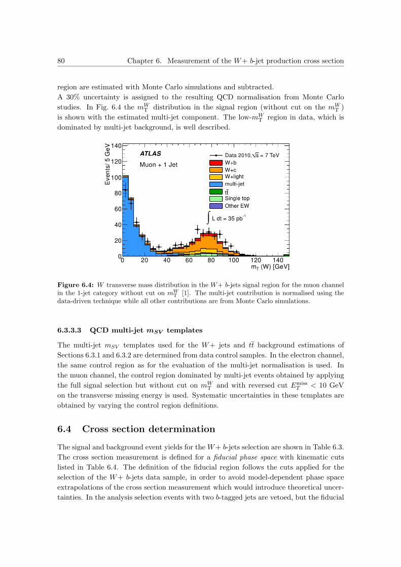
80 Chapter 6. Measurement of the W+ b-jet production cross section
region are estimated with Monte Carlo simulations and subtracted.
A 30% uncertainty is assigned to the resulting QCD normalisation from Monte Carlo
studies. In Fig. 6.4 the mWT distribution in the signal region (without cut on the mW
T )
is shown with the estimated multi-jet component. The low-mWT region in data, which is
dominated by multi-jet background, is well described.
Figure 6.4: W transverse mass distribution in the W+ b-jets signal region for the muon channelin the 1-jet category without cut on mW
T [1]. The multi-jet contribution is normalised using thedata-driven technique while all other contributions are from Monte Carlo simulations.
6.3.3.3 QCD multi-jet mSV templates
The multi-jet mSV templates used for the W+ jets and tt background estimations of
Sections 6.3.1 and 6.3.2 are determined from data control samples. In the electron channel,
the same control region as for the evaluation of the multi-jet normalisation is used. In
the muon channel, the control region dominated by multi-jet events obtained by applying
the full signal selection but without cut on mWT and with reversed cut Emiss
T < 10 GeV
on the transverse missing energy is used. Systematic uncertainties in these templates are
obtained by varying the control region definitions.
6.4 Cross section determination
The signal and background event yields for the W+ b-jets selection are shown in Table 6.3.
The cross section measurement is defined for a fiducial phase space with kinematic cuts
listed in Table 6.4. The definition of the fiducial region follows the cuts applied for the
selection of the W+ b-jets data sample, in order to avoid model-dependent phase space
extrapolations of the cross section measurement which would introduce theoretical uncer-
tainties. In the analysis selection events with two b-tagged jets are vetoed, but the fiducial

6.4. Cross section determination 81
Table 6.3: Event yields in the 1 and 2-jet categories of the electron and muon channels [1]. Forthe W+b, W+c, W+light-quark jets contributions, the Monte Carlo predictions are compared tothe mSV fit results with statistical errors only. The tt and multi-jet contributions are normalisedusing data-driven techniques. All other background contributions are estimated from simulations.
W → µν, 1-jet W → µν, 2-jet W → eν, 1-jet W → eν, 2-jet
Pred. Fit result Pred. Fit result Pred. Fit result Pred. Fit result
W+b-jets 25 28± 13 26 62± 18 18 33± 12 19 38± 14W+c-jets 108 170± 20 45 54± 19 84 105± 18 36 24± 15
W+ light-jets 38 21.2± 9.9 20 21± 10 30 22± 10 17 14.4± 7.7multi-jet 8 - 10 - 10 - 5.8 -
tt 11 - 44 - 8.1 - 33 -single-top 17 - 23 - 14 - 18 -
Other backgrounds 3.9 - 2.5 - 1.9 - 2.1 -
Total Predicted 212 - 170 - 167 - 131 -
Data 261 217 194 136
region for the cross section is defined for events with at least one b-jet. This means that
the fiducial cross section measurement for the 2-jet category is defined for events with a
b-jet and a second jet that can either be a b-jet (which in the data sample is not tagged
due to the inefficiency of the SV0 tagger) or a c or light-jet.
Table 6.4: Fiducial phase space for the W+ b-jets analysis. A jet is identified as a b-jet if it ismatched to a b-hadron quark with pT > 5 GeV within ∆R = 0.3.
Variable Cut
W → eν/W → µν selection
W → τν → e/µννν decays ExcludedLepton momentum pT > 20 GeVLepton pseudo-rapidity |η| <2.5Neutrino pT > 25 GeVW transverse mass mW
T > 40 GeV
Jets
Jet momentum pT > 25 GeVJet rapidity |y| <2.1Jet multiplicity 1 ≤ n ≤ 2b-jet multiplicity n ≥ 1
Jet-lepton isolation ∆R(jet, l) > 0.5
The W+ b-jets cross section is determined separately for the electron and the muon chan-
nels and in the 1 and 2-jet categories according to
σfidW+ b-jet ×BR(W → `ν) =NW+ b-jets
Ufid ·∫Ldt
(6.5)
where NW+ b-jets is the W+ b-jets events yield measured in data (see Table 6.3), Ufid the
signal selection efficiency in the fiducial phase space and∫Ldt the integrated luminosity

82 Chapter 6. Measurement of the W+ b-jet production cross section
of the data set.
The selection efficiency Ufid is determined in Alpgen+HerwigW+ jets simulated events
with the equation
Ufid =nMC,reco
nW+ b-jets,fidMC,true
. (6.6)
where nMC,reco is the number of reconstruction level events (i.e. Monte Carlo events after
full simulation of the detector response) passing the analysis selection and nW+ b-jets,fidMC,true the
number of generated W+ b-jets events which are in the fiducial region of the measurement.
The jets at generator level are built using the anti-kT algorithm with a distance parameter
of R = 0.4 on the 4-momenta of generated stable particles (see Section 4.4). A generator
level jet is identified as a true b-jet if matched to a b-hadron with pT > 5 GeV within
∆R = 0.3. The same b-hadron matching is also applied to the jets at reconstruction level,
to ensure that Ufid is evaluated only for signal events. The possible bias introduced by
this convention has been studied by using b quarks instead of the hadrons for the matching
and found to be negligible.
At generator level the momentum of the electron/muon produced in the W → e/µν decay
is evaluated including the momenta of all final state radiation photons within a ∆R = 0.1
cone (dressed momentum).
The W → τν → e/µννν decays, which are explicitly vetoed in the denominator of Ufid
since they are not included in the fiducial region, give a small contribution at reconstruction
level. They are included in the numerator of Ufid to correct for the small contribution of
these decays in the data sample. The numerator is therefore defined as
nMC,reco = nW→e/µνMC,reco + n
W→τν→e/µνννMC,reco .
The final results on the selection efficiency are presented in Table 6.5.
Table 6.5: Selection efficiency within the fiducial region for the cross section measurement. Onlystatistical uncertainties are shown.
Jet category nW→e/µνMC,reco n
W→τν→e/µνννMC,reco nW+ b-jets,fid
MC,true Ufid [%]
Electrons1 17.64±0.84 0.276±0.078 108.1±2.2 16.57±0.852 18.15±0.69 0.73 ±0.15 91.1±1.6 20.72±0.86
Muons1 24.2 ±1.0 0.61 ±0.16 107.0±2.1 23.2 ±1.12 25.53±0.84 0.374±0.091 91.7±1.6 28.2 ±1.0

6.5. Systematic uncertainties 83
6.5 Systematic uncertainties
In this section the systematic error estimation is described, which has the following con-
tributions.
b-tagging efficiency
The uncertainty in the efficiency of the SV0 b-jet tagging algorithm represents one of the
biggest systematic uncertainties for the measurement. It has been measured to be between
6% and 13% depending on the jet pT [78].
mSV templates
The uncertainty in the mSV templates used for the data-driven background normalisation
described in Section 6.3.1 is another important source of systematic error. The systematic
errors in the mSV templates for b-jets, c-jets and light-quark jets obtained from Monte
Carlo events are determined comparing data and simulation in control regions enriched
with the respective quark flavours.
tt background
There are two sources of uncertainty in the tt background estimation described in Sec-
tion 6.3.2, the uncertainty in the tt yield in the control region and the uncertainty in the
extrapolation of this yield from the control to the signal region. The first one is dominated
by limited data statistics, the second one has a significant contribution from the jet energy
scale uncertainty. Uncertainties due to the Monte Carlo modelling of the tt production
process are also considered, in particular the uncertainties on the PDFs and in the de-
scription of the initial and final state radiation and on the differences in the description
of tt events from different Monte Carlo generators.
Single-top background
The single-top background is estimated from Monte Carlo simulation. A 10% uncertainty
is attributed to the theoretical uncertainties on the cross section, determined by varying
the factorization and renormalisation scales by a factor 2 and considering the PDF un-
certainties. Another source of error in the normalisation of the single-top background is
the description of the initial and final state radiation in the Monte Carlo simulation. Un-
certainties on the estimated single-top contribution due to detector effects are also taken
into account.
Signal modelling
The uncertainties in the description of the signal process in the Monte Carlo simulation
are determined studying the effects of variations of the shapes of the b-jet spectrum and

84 Chapter 6. Measurement of the W+ b-jet production cross section
of the bb pair opening angle distribution on the selection efficiency. Two extreme cases are
considered: distributions fully modelled by the matrix elements and distributions obtained
from the parton shower description.
Multi-jet background estimation
As described in Section 6.3.3, in the electron channel the uncertainty in the measure-
ment of the QCD background normalisation is 50%, mostly due to limited data statistics.
Systematic variations of the normalisation and of the multi-jet mSV template have been
studied modifying the definition of the control region used for the background estima-
tion. In the muon channel the uncertainty in the normalisation is 30%, which has been
determined studying the matrix method used for the background estimation in simulated
samples. Uncertainties in the mSV template have been studied by varying the control
region definition in the muon channel as well.
Jet energy uncertainties
Uncertainties in the jet energy scale and the jet energy resolution assessed in [73] affect
the signal selection efficiency.
Lepton reconstruction uncertainties
The measured uncertainties in the lepton trigger, reconstruction and isolation cut effi-
ciencies as well as the lepton momentum scales and resolutions [71, 92] affect the signal
selection efficiency.
EmissT uncertainty
Variations in the lepton and jet momenta are propagated to the measured missing trans-
verse energy. An additional uncertainty is attributed to the contribution of soft jets, with
pT < 20 GeV to the EmissT [79].
Luminosity error
The 35.5 pb−1 dataset used for the analysis has an uncertainty in the luminosity measure-
ment of 3.4% [94].
Pile-up effects
The uncertainty due to the presence of jets generated by pile-up collisions is estimated from
the variation of the yields when the cut on the jet vertex fraction described in Section 6.2
is removed.

6.6. Results of the fiducial cross section measurement 85
6.6 Results of the fiducial cross section measurement
The cross section measured in the fiducial phase space region defined in Table 6.4 for the
production of a leptonically decaying W in association with one b-jet and a maximum
of one additional jet of any flavour are given in Table 6.6 separately for the W → eν
and W → µν channels for the 1-jet and 2-jet event categories. The cross section are
determined for the combination of the two leptonic channels by averaging the individual
results and for the combination of the two jet categories summing linearly the individual
measurements. Most of the systematic uncertainties are correlated between the channels
and the event categories.
Table 6.6: Fiducial cross section for the production of a leptonically decaying W boson in asso-ciation with at least one b-jet for events with 1 and 2 jets and their combination and breakdownof the contributions to the systematic error [1]. The fiducial region of the measurement is given inTable 6.4.
Fiducial cross section [pb]
Event category 1 jet 2 jet 1+2 jet
Lepton channel µ e µ & e µ e µ & e µ e µ & e
Measured cross section 3.5 5.5 4.5 6.2 5.1 5.7 9.7 10.7 10.2
Statistical uncertainty 1.6 2.1 1.3 1.8 1.9 1.3 2.4 2.8 1.9Systematic uncertainty 1.1 1.7 1.3 1.5 1.5 1.4 2.4 3.0 2.6
Breakdown of systematic uncertainty [%]
b-tagging efficiency 15 14 14 10 10 10 11 12 12Template shapes 16 13 12 10 12 10 11 11 10tt 9 6 7 12 16 13 11 11 11single-top 10 6 8 4 6 5 7 6 6Signal modelling 9 8 9 10 10 10 9 9 9Multi-jet 7 18 11 4 8 4 5 13 7Jet uncertainties 9 6 7 7 10 8 7 7 7Lepton uncertainties 3 5 3 2 5 3 2 5 3EmissT 1 1 1 2 2 1 1 1 1
Luminosity 5 5 5 4 5 5 5 5 5Multiple interactions 5 4 5 3 3 3 3 4 3
The theoretical predictions for the fiducial cross section [95] are shown in Table 6.7 and
compared to the measurements in this thesis in Figure 6.5. The theoretical predictions
have been performed at next-to-leading order (NLO) in the 5 flavours number scheme
(5FNS), i.e. considering production diagrams with b quarks in the initial state. The pop-
ulation of b quarks in the initial state is described by a parton density function (PDF).
The experimental results are in agreement with the theoretical predictions within the un-
certainties. The results in the 2-jet category indicate an excess of the measurement of

86 Chapter 6. Measurement of the W+ b-jet production cross section
5.7±1.9 pb above the prediction 1.9+0.8−0.4 pb. The results of a subsequent ATLAS mea-
surement of the W+ b-jets cross section with the larger 2011 dataset [96] do not confirm
this discrepancy. The 2011 measurement for the 2-jet category of 2.2±0.5 pb, in a fiducial
region slightly different from the one adopted for the 2010 analysis presented in this thesis,
is in good agreement with the NLO prediction of 1.7+0.5−0.3 pb [96] calculated with the Monte
Carlo software MCFM [40] in the 5FNS.
Table 6.7: [95] NLO QCD predictions for the W+ b-jets cross section in the fiducial phaseregion of the measurement (see Table 6.4) [95]. Theoretical errors are due to the uncertainty inthe renormalisation and factorization scale (SC), in the parton density functions estimates (PDF),in the uncertainty in the b mass (mb) and in the non-perturbative corrections (NP).
Category Fiducial cross section (NLO) [pb]
1-jet 2.9+0.4−0.4 (SC) +0.2
−0.0 (PDF) +0.2−0.1 (mb) ± 0.2 (NP)
2-jet 1.9+0.8−0.4 (SC) +0.1
−0.0 (PDF) +0.1−0.1 (mb) ± 0.1 (NP)
1+2-jet 4.8+1.2−0.7 (SC) +0.3
−0.0 (PDF) +0.3−0.2 (mb) ± 0.3 (NP)

6.6. Results of the fiducial cross section measurement 87
Figure 6.5: Measured cross sections with statistical and total errors [1] in comparison with thetheoretical prediction evaluated in the 5 flavour number scheme [95], where the yellow band repre-sents the total uncertainty. The cross sections predicted by the Alpgen+Herwig+Jimmy MonteCarlo generator using ME+PS and ME only (see Sections 2.1 and 6.1.1), and by Pythia are alsoshown.

88 Chapter 6. Measurement of the W+ b-jet production cross section

Chapter 7
Measurement of the W+ c-jet
production cross section
In this chapter a measurement of the production cross section of a W boson in association
with a single c quark jet (W+ c-jet) with the ATLAS detector is presented [2]. This
process is sensitive to the s quark content of the proton. Measurements of the cross sec-
tion can be used to constrain the s quark PDF. Such measurements have already been
performed at the Tevatron [97] and at the LHC [98], but with uncertainties too large for
using them for PDF determination. Recently preliminary cross section measurements of
W + c production have been published by ATLAS [99] and CMS [100].
The measurement presented in this chapter is the result of the efforts of a very small
analysis team. The main contribution of this work is the calibration of the c-jet tagger
and the measurement of the muon reconstruction efficiency, the signal event selection
including measurement of the selection efficiency and the cross section determination with
the assessment of the systematic uncertainties.
7.1 Motivation
An introduction to W+ jets production at the LHC has been given in Chapter 2. The
Feynman diagrams of the dominant processes for the W+ c-jet production at the LHC are
shown in Figure 7.1. Due to the small values of the CKM matrix elements Vub and Vcb,
the process with a s quark in the initial state dominates. Therefore the W+ c-jet cross
section measurement is sensitive to the s quark content of the proton.
It was introduced in Section 2.1 that the quantum numbers of the proton are determined
by its valence quarks, two u and one d quarks, while quark pairs of all flavours (sea quarks)
are produced inside the proton by the gluons exchanged between the valence quarks. The
contributions of the gluons and of the different quark flavours to the proton momentum are
described by parton density functions (PDFs). The densities of s/s and of u and d quarks
89
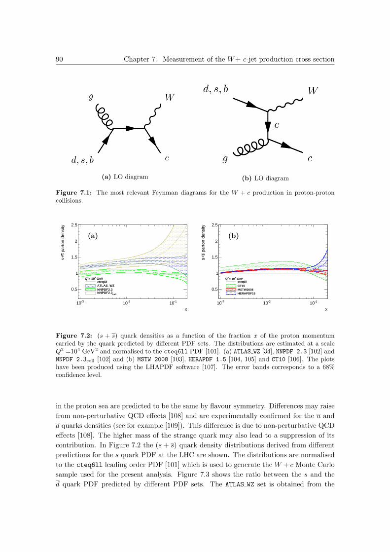
90 Chapter 7. Measurement of the W+ c-jet production cross section
(a) LO diagram (b) LO diagram
Figure 7.1: The most relevant Feynman diagrams for the W + c production in proton-protoncollisions.
x
-310 -210 -110
par
ton
dens
itys
s+
0.5
1
1.5
2
2.5
GeV4= 102Qcteq6llATLAS_WZNNPDF2.3
collNNPDF2.3
(a)
x
-310 -210 -110
par
ton
dens
itys
s+
0.5
1
1.5
2
2.5
GeV4= 102Qcteq6llCT10MSTW2008HERAPDF15
(b)
Figure 7.2: (s + s) quark densities as a function of the fraction x of the proton momentumcarried by the quark predicted by different PDF sets. The distributions are estimated at a scaleQ2 =104 GeV2 and normalised to the cteq6ll PDF [101]. (a) ATLAS WZ [34], NNPDF 2.3 [102] andNNPDF 2.3coll [102] and (b) MSTW 2008 [103], HERAPDF 1.5 [104, 105] and CT10 [106]. The plotshave been produced using the LHAPDF software [107]. The error bands corresponds to a 68%confidence level.
in the proton sea are predicted to be the same by flavour symmetry. Differences may raise
from non-perturbative QCD effects [108] and are experimentally confirmed for the u and
d quarks densities (see for example [109]). This difference is due to non-perturbative QCD
effects [108]. The higher mass of the strange quark may also lead to a suppression of its
contribution. In Figure 7.2 the (s + s) quark density distributions derived from different
predictions for the s quark PDF at the LHC are shown. The distributions are normalised
to the cteq6ll leading order PDF [101] which is used to generate the W + c Monte Carlo
sample used for the present analysis. Figure 7.3 shows the ratio between the s and the
d quark PDF predicted by different PDF sets. The ATLAS WZ set is obtained from the
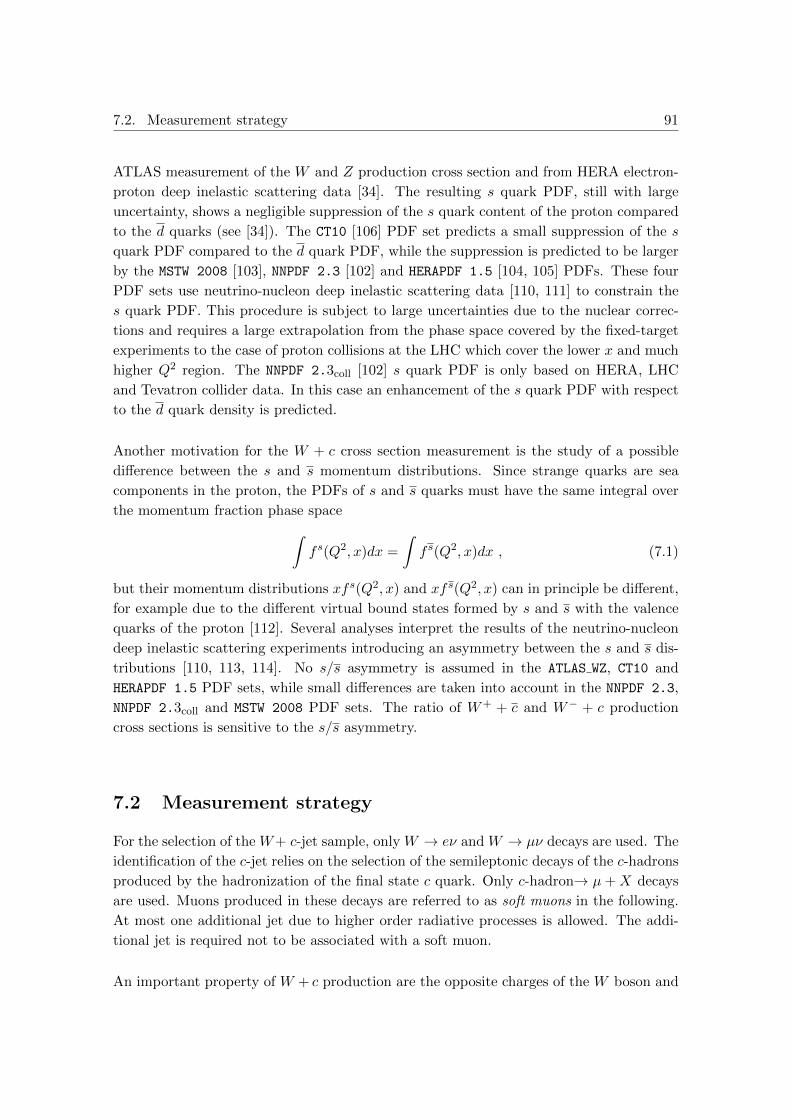
7.2. Measurement strategy 91
ATLAS measurement of the W and Z production cross section and from HERA electron-
proton deep inelastic scattering data [34]. The resulting s quark PDF, still with large
uncertainty, shows a negligible suppression of the s quark content of the proton compared
to the d quarks (see [34]). The CT10 [106] PDF set predicts a small suppression of the s
quark PDF compared to the d quark PDF, while the suppression is predicted to be larger
by the MSTW 2008 [103], NNPDF 2.3 [102] and HERAPDF 1.5 [104, 105] PDFs. These four
PDF sets use neutrino-nucleon deep inelastic scattering data [110, 111] to constrain the
s quark PDF. This procedure is subject to large uncertainties due to the nuclear correc-
tions and requires a large extrapolation from the phase space covered by the fixed-target
experiments to the case of proton collisions at the LHC which cover the lower x and much
higher Q2 region. The NNPDF 2.3coll [102] s quark PDF is only based on HERA, LHC
and Tevatron collider data. In this case an enhancement of the s quark PDF with respect
to the d quark density is predicted.
Another motivation for the W + c cross section measurement is the study of a possible
difference between the s and s momentum distributions. Since strange quarks are sea
components in the proton, the PDFs of s and s quarks must have the same integral over
the momentum fraction phase space∫fs(Q2, x)dx =
∫f s(Q2, x)dx , (7.1)
but their momentum distributions xfs(Q2, x) and xfs(Q2, x) can in principle be different,
for example due to the different virtual bound states formed by s and s with the valence
quarks of the proton [112]. Several analyses interpret the results of the neutrino-nucleon
deep inelastic scattering experiments introducing an asymmetry between the s and s dis-
tributions [110, 113, 114]. No s/s asymmetry is assumed in the ATLAS WZ, CT10 and
HERAPDF 1.5 PDF sets, while small differences are taken into account in the NNPDF 2.3,
NNPDF 2.3coll and MSTW 2008 PDF sets. The ratio of W+ + c and W− + c production
cross sections is sensitive to the s/s asymmetry.
7.2 Measurement strategy
For the selection of the W+ c-jet sample, only W → eν and W → µν decays are used. The
identification of the c-jet relies on the selection of the semileptonic decays of the c-hadrons
produced by the hadronization of the final state c quark. Only c-hadron→ µ+X decays
are used. Muons produced in these decays are referred to as soft muons in the following.
At most one additional jet due to higher order radiative processes is allowed. The addi-
tional jet is required not to be associated with a soft muon.
An important property of W + c production are the opposite charges of the W boson and

92 Chapter 7. Measurement of the W+ c-jet production cross section
x
-310 -210 -110
par
ton
dens
ityd
)/2
s(s
+
0
0.2
0.4
0.6
0.8
1
1.2
1.4
GeV4= 102QATLAS_WZNNPDF2.3
collNNPDF2.3
(a)
x
-310 -210 -110
par
ton
dens
ityd
)/2
s(s
+
0
0.2
0.4
0.6
0.8
1
1.2
1.4
GeV4= 102QCT10MSTW2008HERAPDF15
(b)
Figure 7.3: Average of the s and s parton densities divided by the d quark PDF as a functionof the fraction x of the proton momentum carried by the quark predicted by different PDF sets.The distributions are estimated at a scale Q2 =104 GeV2. (a) ATLAS WZ [34], NNPDF 2.3 [102] andNNPDF 2.3coll [102] and (b) MSTW 2008 [103], HERAPDF 1.5 [104, 105] and CT10 [106]. The plotshave been produced using the LHAPDF software [107]. The uncertainties are not shown.
the c quark. The charge of the c quark is identified by the charge qsoft−µ of the soft muon
while the charge of the W boson is identified by the charge qW−lep of its decay lepton
as illustrated in Figure 7.4. The selected events are classified into the same sign (SS) or
opposite sign (OS) categories if qW−lepqsoft−µ =1 or qW−lepqsoft−µ = −1, respectively.
Signal events contribute only to the OS category by definition while background events are
almost equally divided between the SS and OS categories. For this reason, the numbers
of OS and SS events selected as discussed in Section 7.4 are subtracted from each other
defining the difference
NOS−SS ≡ NOS −NSS = NOSsignal +NOS
background −NSSbackground . (7.2)
in which most background contributions cancel and the signal contribution is enhanced,
since NOSbackground ≈ NSS
background. Simulation predicts about 80% signal contribution to
NOS−SS . The following background processes are considered:
W+ light-jets production, where soft muons inside jets are mostly non-prompt muons
from pion and kaon decays. This process gives a higher contribution to the OS than
to the SS category due to the production diagrams with u/d-gluon fusion which also
result in opposite charges for the hard lepton and the soft muon. Therefore this
background is still sizeable after the NOS −NSS subtraction.
QCD multi-jet background also has a larger OS than SS component, since both the
selected hard lepton and the soft muon in bb and cc events likely originate from the
two heavy flavour particles in the final state which have opposite charges.

7.2. Measurement strategy 93
Figure 7.4: Diagram of W + c production and decay. The lepton from the W decay and thesoft muon from c quark decay, which have opposite charge, are indicated as well as the jet (yellowcone) containing the soft muon.
The Z+ jets production background is very small in the electron channel but it is
significant in the muon channel where the muon pairs from Z → µµ decay may be
misidentified as a lepton from a W and a soft muon. Z+ jets background contribute
mostly to the OS category and the NOS − NSS subtraction does not neglect its
contribution. Fortunately, most muons of this kind are isolated, and therefore not
matched with a jet.
W + bb and W + cc events may produce a signature similar to the signal one, with
a leptonically decaying W and a soft muon produced by an heavy-flavour hadron,
but these events are evenly divided between the OS and SS categories, thus their
contribution is negligible after the NOS −NSS subtraction.
The tt and single-top backgrounds have relatively small cross sections and their
contribution is expected to be small after the NOS −NSS subtraction.
Diboson production (WW,WZ,ZZ) has a larger OS than SS component, but the
low cross sections, the leptonic branching ratios of the bosons and the isolation of
the leptons result in a very small background contribution.

94 Chapter 7. Measurement of the W+ c-jet production cross section
7.3 Samples used for the analysis
The analysis is performed for 4.64 fb−1 of proton-proton collision at√
s = 7 TeV data
collected by the ATLAS detector during 2011.
A Monte Carlo simulated sample of the W + c signal events is used to determine the
selection efficiency for the determination of the fiducial cross section (see Section 7.9).
The small contributions of tt, single-top, diboson and Z+ jets (in the electron channel)
are estimated with Monte Carlo simulation as well. W + bb and W + cc contributions are
predicted by Monte Carlo simulations to be negligible after the NOS −NSS subtraction.
The contribution of Z+ jets events in the muon channel and of W+ light-jets production
do not vanish after the subtraction and are therefore evaluated with data-driven methods.
The QCD multi-jet background is completely estimated from data.
The simulated event samples and the cross section calculations used for their normalisation
are listed in Table 7.1. The Alpgen [47] generator was used for the simulation of the signal
and of the W +cc, W +bb and W+ light-jets background processes. Pythia [43] was used
for the parton shower (PS) simulation in the signal sample because it was found to describe
better the c hadronization than Herwig. For W + cc, W + bb and W+ light-jets events
Herwig [45] was used as PS algorithm, since higher statistics samples were available.
MC@NLO [49] was used for the tt background simulation, Herwig [45] for the WW , WZ
and ZZ production. The single-top background in the t and Wt-channels was simulated
with AcerMC [51] while the s-channel was simulated with MC@NLO. For the Z+ jets
background, Alpgen+Herwig samples were used.
The MLM [90] and HFOR overlap removal procedures described in Section 6.1.1 were used
for the W+ jets sample.
Table 7.1: Monte Carlo event samples used for the W+ c-jet cross section measurement. Thetotal cross section of the four W+ jets samples is normalised to the NNLO inclusive W productioncross section calculated in [33].
Physics process Generators PDF set σ·BR (nb)
W (→ lν) +c Alpgen [47]+Pythia [43] cteq6ll [101]W (→ lν) +jets Alpgen [47]+Herwig [45] cteq6ll [101]
W (→ lν) +bb Alpgen [47]+Herwig [45] cteq6ll [101]W (→ lν) +cc Alpgen [47]+Herwig [45] cteq6ll [101]
Total W→ lν + jets 10.46 NNLO [33]
Z(→ ll) +jets Alpgen [47]+Herwig [45] cteq6ll [101] 1.07 NNLO [33]WW Herwig [45] MRSTMCal [115] 44.9 × 10⁻³ NLO [40]WZ Herwig [45] MRSTMCal [115] 18.5 × 10⁻³ NLO [40]ZZ Herwig [45] MRSTMCal [115] 5.96 × 10⁻³ NLO [40]tt MC@NLO [49]+Herwig [45] CT10 [106] 90.5 × 10⁻³ approx.NNLO [85]single-top (t-channel) AcerMC[51]+Pythia [43] CT10 [106] 64.6 × 10⁻³ NNLO [116]single-top (s-channel) MC@NLO [49]+Herwig [45] MRSTMCal [115] 4.6 × 10⁻³ NNLO [117]single-top (Wt) MC@NLO [49]+Herwig [45] CT10 [106] 15.7 × 10⁻³ NNLO [118]

7.4. Event selection 95
7.4 Event selection
The event selection criteria are summarised in Table 7.2. The selection is analogous to the
one used for the W+ b-jets cross section measurement discussed in Section 6.2, with cuts
updated for the 2011 data taking conditions and optimized for the background rejection.
For the c-jets a different tagging technique is used based on soft muons reconstructed
inside the jets.
7.4.1 Preselection
Only data have been used where all ATLAS detector subsystems were fully operational.
The primary vertex of the event is required to have at least 3 associated ID tracks in order
to avoid contamination by cosmic muon events.
A reweighting procedure is applied to the Monte Carlo events such that the distributions
of the average number of interactions per bunch crossing < µ > and of the z coordinate
of the primary vertex match the data. The procedures are analogous to the ones applied
in Section 5.1.4 for the muon reconstruction efficiency measurement.
7.4.2 Trigger requirements
The least stringent unprescaled trigger requirements were used. They varied from the early
data taking period, with relatively low instantaneous luminosity, to the late period with
higher instantaneous luminosity and pile-up levels. For the electron channel the following
trigger conditions are applied [119]:
EF e20 medium in the early data taking period requiring an electron with pT > 20 GeV
of medium quality (see Section 4.3).
EF e22 medium in the intermediate period requiring an electron of medium quality
with pT > 22 GeV.
EF e22vh medium in the late data taking period requiring an electron with pT > 22 GeV
of medium quality and with a veto on energy deposits higher than 1 GeV in the
hadronic calorimeter in a ∆η ×∆φ = 0.2× 0.2 window around the electron.
For the muon channel, the following trigger requirements are used [88]:
EF mu18 in the early data taking period requiring a muon with pT > 18 GeV seeded
by a level-1 trigger muon candidate with pT > 10 GeV (see Section 3.2.6.1).
EF mu18 medium in the late data taking period requiring a muon with pT > 18 GeV
seeded by a level-1 trigger muon candidate with pT > 11 GeV.

96 Chapter 7. Measurement of the W+ c-jet production cross section
The leptons selected by the trigger algorithms are required to match within ∆R = 0.15
the leptons reconstructed offline to ensure that no bias is introduced by the trigger.
The Monte Carlo simulations are reweighted to correctly describe the varying trigger
conditions in data [88, 119].
7.4.3 Lepton selection
Different pT cuts are applied for electrons (pT > 25 GeV) and muons (pT > 20 GeV)
because of the different trigger conditions. The values are chosen to lie in the plateau re-
gion of the trigger efficiency. All leptons are required to be inside the trigger acceptance:
|η| <2.47 (without 1.37 < |η| < 1.52) for electrons and |η| < 2.4 for muons.
In order to reject the QCD multi-jet background, the leptons are required to be isolated.
A multi-lepton veto is applied in both channels to reject background processes.
7.4.3.1 Electron channel
The tight++ electron identification (see Section 4.3) is used for electron selection. A loose
cut on the transverse impact parameter of the electron is applied to ensure that it is com-
ing from the reconstructed primary vertex. The calorimeter energy in a ∆R = 0.3 cone
around the electron is required to be less than 3 GeV.
A veto is applied against additional electrons fulfilling a looser selection criteria: medium++
identification and pT > 20 GeV within |η| <2.47 (without 1.37 < |η| < 1.52). To re-
ject diboson and tt backgrounds, a veto is applied against combined muons reconstructed
with Staco (see Section 4.7) and with pT > 20 GeV, |η| < 2.5 and z0 < 10 mm,
satisfying the quality requirements in Table 5.3 and passing a track isolation cut of∑∆R=0.2 ptracksT /pT < 0.1.
7.4.3.2 Muon channel
Combined muons reconstructed with Muid (see Section 4.7) passing the kinematic cuts
mentioned above are selected. The quality cuts of Table 5.3 are applied to the Inner
Detector (ID) tracks associated to the muons. Track and calorimeter isolation criteria∑∆R=0.3 ptracksT < 2.5 GeV and∑∆R=0.2EcaloT < 4 GeV, respectively, are applied.
Events with more than one selected muon are rejected. To reject diboson and tt back-
grounds a veto is applied against tight++ electrons with ET > 25 GeV, |η| < 2.47
(without 1.37 < |η| < 1.52) fulfilling η and pT dependent ID and calorimeter isolation
requirements with 90% efficiency.

7.4. Event selection 97
7.4.3.3 Lepton-jet overlap removal
The jet closest to the signal lepton within ∆R = 0.2 is removed as it may be a fake
jet reconstructed due to the calorimeter activity from the signal lepton. Furthermore,
electrons within ∆R = 0.5 of a jet with pT > 25 GeV and muons within ∆R =0.4 of a
jet with pT > 25 GeV and JVF > 0.75 (see section 7.4.5) are rejected.
7.4.3.4 Lepton efficiency corrections
Corrections are applied to the lepton trigger, reconstruction and isolation efficiencies in
the simulations to fit the data. The corrections presented in Chapter 5 are used for the
muon reconstruction efficiency. Corrections for the the muon isolation and trigger efficien-
cies are evaluated with a Tag-and-Probe method analogous to the one used in Section 5.2.
The electron reconstruction and identification efficiency measurements are described in [72].
Corrections for the electron isolation and impact parameter cut efficiencies are evaluated
with a Tag-and-Probe method analogous to the one described for the muons.
The muon momentum and electron energy scales and resolutions are also corrected in the
simulations to match the data (see [72, 83]).
7.4.4 W boson selection
Only events with a reliable evaluation of the missing transverse energy EmissT are kept (so-
called EmissT cleaning). Events with a jet with pT > 20 GeV failing the looser reconstruction
quality criteria (see Section 4.4) and events with jets falling into the calorimeter region
damaged in 2011 or containing noise bursts in the LAr calorimeter are rejected. An
EmissT > 25 GeV cut is applied in the electron channel which is lowered to 20 GeV in
the muon channel. The lepton and the reconstructed EmissT are used to determine the
transverse mass mWT of the W boson using Eq. 6.1. A mW
T > 40 GeV cut is applied in the
electron channel which is raised to 60 GeV in the muon channel. The difference between
the cuts applied in the two channels is justified by the different backgrounds contamination
especially due to QCD multi-jet events. The cuts are optimized for maximum background
rejection.
7.4.5 Jet selection
The anti-kT algorithm (see Section 4.4) with a distance parameter R = 0.4 is used for
jet reconstruction. Jets are reconstructed from calorimeter clusters at the electromagnetic
energy scale and then recalibrated to the hadronic energy scale and corrected for pile-up
effects [73]. A jet pT cut of 25 GeV is applied. The jets are required to be in the fiducial
region of the c-jet tagger of |η| < 2.5. A JV F > 0.75 cut (see Section 6.2.5) is applied on
the jet vertex fraction to remove jets produced by pile-up interactions. Events are required
to contain one or two jets and are classified in the 1 and 2-jet categories, respectively.

98 Chapter 7. Measurement of the W+ c-jet production cross section
Table 7.2: Event selection criteria for the W+ c-jet cross section measurement
Cut W → eν channel W → µν channel
Preselection
Data taking conditions All sub-detectors working
Primary vertex nPVtracks ≥ 3
Trigger conditionsEF e20 medium[119] (early) EF mu18[88] (early)
EF e22 medium[119] (medium) EF mu18 medium[88] (late)EF e22vh medium[119] (late)
Trigger matching Offline reconstructed lepton within ∆R = 0.15 to trigger lepton
W selection
Lepton identification Tight++CB muon,
quality cuts in Table 5.3
Kinematic cutsET > 25 GeV pT > 20 GeV|η| < 2.47 |η| < 2.4
|η| < 1.37 or |η| > 1.52
Impact parameter cuts d0/σd0 < 10
Lepton isolation
∑∆R=0.3EcaloT < 3 GeV∑∆R=0.2EcaloT < 4 GeV∑∆R=0.3 ptracksT < 2.5 GeV
Lepton-jet overlap removal See text
Lepton-jet isolation See text
Electron veto
Veto events with add. medium++ e Veto events with tight++ e
with ET >20 GeV, |η| <2.47, with ET > 25 GeV, |η| < 2.47,
1.37< |η| <1.52 excluded 1.37< |η| <1.52 excluded,∑∆R=0.3Ecalo
T cut @90% eff.∑∆R=0.3ptracksT cut @90% eff.
Muon veto
Veto events with CB µ, Exactly one µ
with pT > 20 GeV, |η| < 2.5, z0 < 10 mm,
quality cuts in Table 5.3,∑∆R=0.2ptracksT /pT < 0.1
EmissT cleaning Looser jet cleaning, no jets in LAr hole (see text), LAr noise cleaning
Missing energy EmissT > 25 GeV Emiss
T > 20 GeV
W transverse mass mWT > 40 GeV mW
T > 60 GeV
Jets selection
Kinematic cuts pT > 25 GeV, |η| <2.5Quality cuts Loose criteria (see Section 4.4 and [73])Pile-up cleaning Jet vertex fraction JVF > 0.75 (see text)Jet multiplicity njets=1 or 2
c-jet selection
SMT taggerExactly one jet within ∆R = 0.5,
exactly one muon satisfying SMT cuts (see Section 5.3)
c-jet cuts #tracks > 3 or EMF >0.8 (see text)
Lepton cuts8 GeV < m(µ, soft µ) < 11 GeV rejected
80 GeV < m(µ, soft µ) < 100 GeV rejected
7.4.6 c-jet selection
The Soft Muon Tagger (SMT) is used to select c-jets. It relies on the muonic decays of
the c-hadrons. Combined muons with pT > 4 GeV and ∆R = 0.5 from the axis of the
jet are selected. They are referred to as soft muons. Further details on the cuts applied
by the SMT and a detailed study of its performance in the data are given in Section 5.3.
The corrections evaluated there are applied to the simulations to match the data. The
tagged jet is required to be associated to only one soft muon, and events with more than
one tagged jet are rejected.

7.5. Background estimation 99
In the muon channel, Z+ jets production is a non-negligible background. A significant
fraction of this background is due to Z dimuon decays in which one of the muons emits a
final state radiation photon which is wrongly reconstructed as a jet and then selected by
the SMT. An additional cut for the jets tagged by the SMT is, therefore, applied in the
muon channel. They are required to either contain at least 3 ID tracks or that the fraction
of their total energy which is measured in the electromagnetic calorimeter (EMF) is less
than 80%. Furthermore, the invariant mass of the hard and the soft muons is required to
differ from the Υ and Z masses by rejecting events with 8 GeV < m(µ, soft-µ) < 11 GeV
or 80 GeV < m(µ, soft-µ) < 100 GeV.
In the Monte Carlo W + c sample additional corrections are applied concerning properties
of the c-hadron. The events are reweighted to take into account most recent measure-
ments of the fractions of different c-hadron species (fragmentation fraction), the fraction
of c-jet momentum carried by the first c-hadron in the jet (fragmentation function) and
the semimuonic branching ratios of the different c-hadron species. More details are given
in Section 7.9.3.
7.5 Background estimation
In the electron channel, QCD multi-jet and W+ light-jets productions are the most impor-
tant backgrounds, since these processes give higher contributions to the number NOS of
selected events in the opposite sign category than to the same sign NSS one. Their residual
contribution after the NOS −NSS subtraction is therefore significant and it is estimated
with data-driven techniques. In the muon channel, in addition to these two processes,
Z+ jets production is also an important background and its contribution is determined
from data. All other backgrounds are estimated from Monte Carlo simulations.
7.5.1 QCD multi-jet background
QCD multi-jet events pass the event selection for the following reasons:
The selected isolated high-pT electron or muon can come from a hadron decay.
Jets and photons may be misreconstructred as electrons.
Soft muons from hadron decays inside a jet may be selected by the Soft Muon Tagger
in QCD multi-jet events.
The cuts on the lepton pT and isolation variables and the EmissT and mW
T cuts ensure
high rejection of multi-jet events, but their production cross section is several orders of
magnitude higher than for the signal one. The influence of QCD multi-jet background on
the cross section measurement is reduced by the NOS−NSS subtraction but not negligible.

100 Chapter 7. Measurement of the W+ c-jet production cross section
Because of the high production cross section and the strong rejection it is impossible to
simulate enough events for a reliable prediction of the impact of QCD multi-jet production
on the measurement. Therefore this contribution has to be entirely determined with data-
driven techniques.
7.5.1.1 Electron channel
The contribution of QCD multi-jet events in the electron channel is estimated with a
technique analogous to the one described for the W+ b-jets cross section measurement in
Section 6.3.3. The EmissT distribution is measured in data applying the selection cuts of
Section 7.4 apart from the cut on EmissT . Two Emiss
T distributions, one for QCD multi-jet
events and one for all other processes, are used in a template fit to the data EmissT distri-
bution to get the size of the multi-jet contribution.
The multi-jet EmissT template is obtained from a data control sample enriched with QCD
multi-jet events by applying the selection cuts without the cut on EmissT and inverting
part of the electron quality requirements and the nominal isolation variable cut, which is
therefore required to be higher than 3 GeV. The medium++ quality cuts (see Section 4.3)
are still applied for the electron identification as well as tight++ cuts which are used for
the electron trigger and, therefore, have to be applied also to the reconstructed electrons
to avoid bias in the selection of the control sample. The tight++ requirements which are
not used by the trigger algorithms, namely a cut on the number of hits of the electron
track in the TRT detector and a cut discriminating electrons from photon conversions, are
inverted in the control sample selection.
Small contributions from other processes than QCD multi-jet in the control region are
estimated with Monte Carlo simulations and subtracted.
The EmissT distributions obtained separately for OS and SS multi-jet events are found to be
in agreement within the uncertainties. A common multi-jet template for both categories
is therefore used in order to reduce the statistical error.
The non-multi-jet EmissT template includes contributions from the W + c signal and from
all other backgrounds and is determined from Monte Carlo simulations.
The fit to the data EmissT distribution is performed in the 10 < Emiss
T < 90 GeV range
separately for OS and SS events to determine the QCD multi-jet contribution separately
for the two event categories. The charge-asymmetry
αQCD =NQCDOS −NQCD
SS
NQCDOS +NQCD
SS
(7.3)
of the QCD multi-jet background is evaluated using the fit results. αQCD has a smaller
uncertainty than the individual event numbers because part of the uncertainties cancels.
The fit result for NQCDSS is also used as input to the fitting procedure described in Sec-
tion 7.5.3 which gives the final estimate of the QCD multi-jet background in the electron

7.5. Background estimation 101
channel.
The variation of αQCD under the following variations is taken as the uncertainty on this
parameter:
The EmissT range in the fit, changing the lower bound between 5-20 GeV and the
higher one between 70-120 GeV.
The multi-jet template is varied by changing the inverted isolation cut between 1-
7 GeV and varying the quality criteria for the electron selection.
The non-multi-jet template is varied by changing the fraction of each contributing
process by 20%.
The effect of the statistical uncertainties in the templates is evaluated using toy Monte
Carlo simulations. The final results for the charge-asymmetry of QCD multi-jet events
with one or two selected jets are
αQCD1−jet,e = 0.025± 0.06 (7.4)
and
αQCD2−jet,e = 0.04± 0.09 . (7.5)
7.5.1.2 Muon channel
In the muon channel, the QCD multi-jet contribution is estimated as
NQCDOS−SS = NQCD
pre−tag ·RQCDSMT · α
QCD (7.6)
where NQCDpre−tag is the number of events passing the selection cuts without the Soft Muon
Tagger cuts and RQCDSMT the tagging rate of the SMT measured for QCD multi-jet events.
NQCDpre−tag is measured with a method analogous to the one presented for the W+ b-jets
cross section measurement in Section 6.3.3. A loose selection is performed by dropping
the muon isolation requirements, the tight selection uses the nominal isolation cuts. The
tight and loose samples both contains contributions of fake non-prompt muons, produced
in QCD multi-jet events, and of real prompt muons. Measuring the selection efficiency
of the tight isolation cut for these two components, NQCDpre−tag can be determined applying
Eq. 6.4. The efficiency εreal of the isolation cuts for prompt muons is determined in a data
sample enriched with Z → µµ events by measuring the fraction of muons passing these
cuts, in analogy with the measurement described in Section 5.2. The efficiency εfake of
the isolation cuts for non-prompt muons is measured in a data control sample enriched
with QCD multi-jet events selected using inverted EmissT and mW
T cuts. To quantify the

102 Chapter 7. Measurement of the W+ c-jet production cross section
uncertainty of εfake an alternative estimation of εfake is performed evaluating the isolation
efficiency as a function of the impact parameter significance d0/σd0 of the muons, since
at high d0/σd0 values muons from c and b decays are dominating. The two methods give
different results for εfake as the second method is more sensitive to heavy flavour produc-
tion in QCD multi-jet events which results in muons with higher d0/σd0 values. εfake is,
therefore, taken as the average of the two results and their difference is used as systematic
uncertainty.
RQCDSMT and αQCD are measured in two different data control samples enriched with QCD
multi-jet events (see Figure 7.5). The first sample is selected by inverting the muon isola-
tion cuts, i.e. by requiring∑∆R=0.2EcaloT > 5 GeV and
∑∆R=0.3 ptracksT > 3.5 GeV. For
the second sample mWT < 30 GeV is required. The contributions of W+ jets and Z+ jets
events in the control regions are estimated from Monte Carlo simulations and subtracted.
A 25% uncertainty including cross section and detector related errors is assigned to this
estimation. All other processes give very small contributions and are thus neglected.
In the two control data samples, RQCDSMT and αQCD are evaluated from the numbers of
events Npre−tag and NSMT before and after the Soft Muon Tagger cuts as
RQCDSMT =NSMTdata −NSMT
W/Z+jets,MC
Npre−tagdata −Npre−tag
W/Z+jets,MC
(7.7)
and
αQCD =(NSMT
data −NSMTW/Z+jets,MC)OS − (NSMT
data −NSMTW/Z+jets,MC)SS
(NSMTdata −NSMT
W/Z+jets,MC)OS + (NSMTdata −NSMT
W/Z+jets,MC)SS. (7.8)
The RQCDSMT and αQCD results obtained in the two control data samples are averaged. The
uncertainty in RQCDSMT is defined as the difference between the two estimates divided by√
2,
which is larger than the uncertainty on the individual measurements. The largest one of
the errors of the two measurements is used as the uncertainty on the average αQCD since
it is larger than the difference between the two measurements.
To refine the estimate of RQCDSMT , a second method has been developed:. In the control
region with inverted isolation cuts, RQCDSMT is found to increase linearly with decreasing
muon isolation cuts, i.e. for less isolated muons. A linear extrapolation of the RQCDSMT val-
ues from the control to the signal region provide results in agreement with the previously
determined values but with smaller uncertainties.
The results of the multi-jet background estimation in the muon channel are summarized
in Table 7.3.

7.5. Background estimation 103
Calorimeter isolation [GeV]
-1 0 1 2 3 4 5 6 7 8
Eve
nts
/ 0.3
GeV
110
210
310
410
510
610
710
810
910
1010
1110
1210
1310
1410 1 jet bin pre-tagνµ →W
W+c
cW+c
bW+bW+light-jets
Z+jets
ttsingle-top
WW,WZ,ZZ
data
Signal region Control region
(a)
Calorimeter isolation [GeV]
-1 0 1 2 3 4 5 6 7 8
Eve
nts
/ 0.3
GeV
110
210
310
410
510
610
710
810
910
1010
1110
1210 1 jet bin OS+SSνµ →W
W+c
cW+c
bW+bW+light-jets
Z+jets
ttsingle-top
WW,WZ,ZZ
dataSignal region Control region
(b)
ID isolation [GeV]
0 1 2 3 4 5 6 7 8 9 10
Eve
nts
/ 0.2
GeV
110
210
310
410
510
610
710
810
910
1010
1110
1210 1 jet bin pre-tagνµ →W
W+c
cW+c
bW+b
W+light-jets
Z+jets
tt
single-top
WW,WZ,ZZ
data
Signal region Control region
(c)
ID isolation [GeV]
0 1 2 3 4 5 6 7 8 9 10
Eve
nts
/ 0.2
GeV
1
10
210
310
410
510
610
710
810 1 jet bin OS+SSνµ →W
W+c
cW+c
bW+b
W+light-jets
Z+jets
tt
single-top
WW,WZ,ZZ
data
Signal region Control region
(d)
[GeV]WTm
0 20 40 60 80 100 120 140
Eve
nts
/ 5 G
eV
210
310
410
510
610
710
810
910
Signal regionControl region
1 jet bin pre-tagνµ →W
W+c
cW+c
bW+b
W+light-jets
Z+jets
tt
single-top
WW,WZ,ZZ
data
(e)
[GeV]WTm
0 20 40 60 80 100 120 140
Eve
nts
/ 5 G
eV
10
210
310
410
510
610
710
Signal regionControl region
1 jet bin OS+SSνµ →W
W+c
cW+c
bW+b
W+light-jets
Z+jets
tt
single-top
WW,WZ,ZZ
data
(f)
Figure 7.5: Selection of two QCD multi-jet enriched control samples for the muon channel usinginverted isolation cuts (a, b, c, d) and an inverted mW
T cut (e, f. The left plots are before SMTcuts, the right plots are after the full selection for the combination of the OS and SS samples.Simulated distributions for the W + c signal and all backgrounds, except QCD multi-jet, areshown in the plots and normalised to the Monte Carlo predictions. Data exceeding the MonteCarlo estimated contributions is assumed to correspond to QCD multi-jet events which are thedominating component in the control regions.

104 Chapter 7. Measurement of the W+ c-jet production cross section
Table 7.3: Variables used for the QCD multi-jet background prediction in the muon channel
1-jet events 2-jet events
NQCDpre−tag,µ 21955 ± 3011 6254 ± 1519
RQCDSMT,µ 0.0144± 0.0048 0.035± 0.010
αQCDµ 0.226 ± 0.038 0.237± 0.044
7.5.2 W+ light-jets background
W+ light-jets events contribute to the background due to mistagged light-jets. Soft muons
inside light-jets likely are from semileptonic decays of π or K mesons which make up almost
all of the tracks inside a jet. Despite the strong rejection of the SMT against light-jets,
W+ light-jets background is important due to the high production cross section. This
process gives a higher contribution to the OS sample than to the SS one and is therefore
not negligible in the NOS −NSS subtraction. Its contribution is determined with a data-
driven method.
7.5.2.1 Electron channel
In the selected data sample without application of the Soft Muon Tagger cuts (pre-tag
data sample) the number of combinations of the electron with tracks in the selected jets
with OS and SS charges are determined in order to measure the OS/SS charge-asymmetry
αW+ light-jetstracks (defined as for Eq. 7.3) for the W+ jets background, which is the dominat-
ing contribution to the pre-tag sample. The QCD multi-jet contribution to this sample
is estimated with the same technique as discussed in Section 7.5.1, all other background
contributions are determined by simulations. The background contributions are then sub-
tracted from the data. The W + c background for the αW+ light-jetstracks measurement is also
estimated in simulations.
The ratio of the charge-asymmetry for tracks and for the nominal selection in Monte
Carlo events αW+ light-jetsMC /αW+ light-jets
MC,tracks is then used to rescale the value of αW+ light-jetstracks
measured in data to determine αW+ light-jets. The results for events with one and two
selected jets are
αW+ light-jets1−jet,e = 0.09± 0.03 (7.9)
and
αW+ light-jets2−jet,e = 0.07± 0.03 , (7.10)
respectively. The asymmetry parameters are used together with the results of the fitting
technique described in Sec. 7.5.3 to determine the W+ light-jets contribution after the
NOS −NSS subtraction in the electron channel.

7.5. Background estimation 105
7.5.2.2 Muon channel
In the muon channel, the W+ light-jets contribution is estimated with a strategy similar
to the one used for the QCD multi-jet background. The W+ light-jets contributions after
the NOS −NSS subtraction is
NW+ light-jetsOS−SS = NW+ jets
pre−tag · fW+ light-jets ·RW+ light-jetsSMT · αW+ light-jets (7.11)
where NW+ jetspre−tag is the number of W+ jets events before the Soft Muon Tagger cuts,
fW+ light-jets the fraction ofW+ light-jets events in the pre-tagW+ jets sample, RW+ light-jetsSMT
the SMT tagging rate in W+ light-jets events and αW+ light-jets the OS/SS charge-
asymmetry of W+ light-jets events (defined as for Eq. 7.3).
The number of pre-tag W+ jets events is determined from data assuming that after sub-
traction of the backgrounds only W+ jets events remain. Diboson, tt and single-top
backgrounds are estimated with Monte Carlo simulations and the QCD multi-jet and
Z+ jets contributions with the methods described in Section 7.5.1 and 7.5.4, respectively.
fW+ light-jets is evaluated using a heavy-flavour jet tagger based on the long lifetime of
c-hadrons and b-hadrons, MV1 [120]. The number of pre-tag W+ jets events which are
tagged by MV1 can be expressed as the sum of the W+ light-jets, W + bb, W + cc and
W + c pre-tag contributions, each one multiplied by the corresponding tagging rate R:
NW+ jets,±MV 1,pre−tag = NW+ jets,±
pre−tag (fW+bbRW+bbMV 1 + fW+ccRW+cc
MV 1
+ fW+cRW+cMV 1 + fW+ light-jetsRW+ light-jets
MV 1 ) ,(7.12)
fW+bb + fW+cc + fW+c + fW+ light-jets = 1 . (7.13)
The tagging rates of MV1 for W+ light-jets, W + bb, W + cc and W + c events are deter-
mined using simulated event samples, with the jet-pT dependent data-driven corrections
to the tagging efficiency evaluated in [120] applied. The fraction of W + bb/W + cc events
is also evaluated in simulations. Considering separately W+ and W− events the equations
can be finally solved to find fW+ light-jets.
The SMT tagging rate RW+ light-jetsSMT is estimated from Monte Carlo simulations with
data-driven correction factors applied (see Section 5.3). The asymmetry αW+ light-jets is
determined as for the electron channel. The final results on the W+ light-jets background
estimation in the muon channel are given in Table 7.4

106 Chapter 7. Measurement of the W+ c-jet production cross section
Table 7.4: Parameters used for the W+ light-jets background estimation in the muon channel
1-jet events 2-jet events
NW+ jetspre−tag,µ 1746273± 5438 365518 ± 2538
fW+ light-jetsµ 0.848 ± 0.068 0.762 ± 0.061
RW+ light-jetsSMT,µ 0.00211 ± 0.00030 0.00578± 0.00082
αW+ light-jetsµ 0.069 ± 0.022 0.023 ± 0.025
7.5.3 Refinement of the QCD multi-jet and W+ light-jets background
determination in the electron channel
In the electron channel the estimations of the QCD multi-jet and W+ light-jets contribu-
tions, discussed in Sections 7.5.1.1 and 7.5.2.1, are the dominating sources of background
uncertainties. The estimate of the size of their contributions is refined using a fitting tech-
nique in the SS sample, after subtraction of all other processes which are estimated from
Monte Carlo, assuming that the difference between prediction and data for SS events can
be totally attributed to QCD multi-jet and W+ light-jets events. The following quantity
is minimized:
χ2 =(Nfit,SS
QCD −NQCD)2
σ2QCD,SS
+(Nfit,SS
W+ light-jets −NSSW+ light-jets)
2
σ2W+ light-jets,SS
, (7.14)
with NSSQCD and NSS
W+ light-jets being the data driven estimates of the QCD multi-jet and
W+ light-jets SS contributions and Nfit,SSQCD and Nfit,SS
W+ light-jets being the refined estimate
of their SS contributions which are constrained by
Nfit,SSW+ light-jets = NSS
data −Nfit,SSQCD −NMC,SS
other processes . (7.15)
The uncertainties σQCD,SS and σW+ light-jets,SS on the estimates of the SS contributions
are determined in simulations as 50% and 30%, respectively.
The Nfit,SSQCD and Nfit,SS
W+ light-jets resulting from the minimization are used together with the
charge-asymmetries αQCD,W+ light-jets estimated in Sections 7.5.1 and 7.5.2 to compute
the contributions of QCD multi-jet and W+ light-jets backgrounds after the NOS −NSS
subtraction by using the equation
NOS−SSQCD,W+ light-jets =
2 · αQCD,W+ light-jets ·NSSQCD,W+ light-jets
1− αQCD,W+ light-jets. (7.16)
The lower impact of the uncertainties in the QCD multi-jet background estimation and
the higher relevance of the Z+ jets background in the muon channel would greatly reduce
the benefits of this method, which is therefore used in the electron channel only.

7.5. Background estimation 107
7.5.4 Z+ jets background
Z+ jets production is a small background in the electron channel, where it is estimated
from simulations, but is important in the muon channel. The analysis selection defines
a dimuon data sample with an isolated hard muon and a soft muon inside a jet. Most
Z+ jets events with a Z → µµ decay are rejected by the dilepton veto applied, which
discards events with two isolated muons. Z+ jets events in which one of the two Z-muons
is not reconstructed by the detector and with a soft muon produced inside one of the jets
contribute equally to the OS and SS sample and their contribution is therefore negligible
after the NOS −NSS subtraction.
On the other hand, events in which one of the Z muons is not isolated, mostly because it
radiates a photon which is misreconstructed as a jet, represent an important background
because they only contribute to the OS sample like the signal events. An additional cut is
applied in the muon channel to the jet tagged by the SMT in order to reduce the contri-
bution of these events. The jet is required either to be associated with at least 3 ID tracks
or to have an electromagnetic fraction (EMF ), i.e. the fraction of its total energy which
is reconstructed in the electromagnetic calorimeter, below 80%. As shown in Figure 7.6
Z+ jets events are characterised on average by a lower track multiplicity nTracks and
and a higher electromagnetic fraction EMF with respect to signal events.
SMT-jet EMF
0 0.1 0.2 0.3 0.4 0.5 0.6 0.7 0.8 0.9 1
Nor
mal
ised
to u
nity
0
0.02
0.04
0.06
0.08
0.1
0.12
0.14
+1 jet OS-SSνµ →W
Z+jets
W+c
Simulation (a)
SMT-jet nTracks
0 5 10 15 20
Nor
mal
ised
to u
nity
0
0.05
0.1
0.15
0.2
0.25
+1 jet OS-SSνµ →W
Z+jets
W+c
+1 jet OS-SSνµ →W
Z+jets
W+c
Simulation(b)
Figure 7.6: Electromagnetic energy fraction EMF (a) and track multiplicity nTracks (b) distri-butions normalised to unity for SMT tagged jet in Monte Carlo Z+ jets (green) and W + c (red)muon channel events No dilepton invariant mass cut is applied to the events in the plots. is notapplied. Only statistical errors are shown.
To further reduce the Z+ jets contribution the difference between the invariant mass of
the hard and soft muons m(µ, soft-µ) and the Z mass is required to be at least 10 GeV
in the muon channel. The 80 GeV < m(µ, soft-µ) <100 GeV region defines a control
sample dominated by Z+ jets production (see Figure 7.7a) which is used to determine the

108 Chapter 7. Measurement of the W+ c-jet production cross section
Z+ jets background with a data driven technique.
[GeV]invm
0 20 40 60 80 100 120
Eve
nts
/ 1.2
GeV
0
20
40
60
80
100
120
140
160
180
200
+1 jet OS-SSνµ →W
Z+jets
W+c
Simulation (a)
[GeV]invm
70 75 80 85 90 95 100 105
Eve
nts
/ 1.2
GeV
0
20
40
60
80
100
120
140
160
180 +1 jet OS-SSνµ →WW+cW+light-jetsZ+jets
ttsingle-topWW,WZ,ZZdata
(b)
Figure 7.7: (a) Distributions of the invariant mass m(µ, soft-µ) of hard and soft muons in MonteCarlo Z+ jets and W + c events after the selection. (b) data m(µ, soft-µ) distribution near theZ peak with the estimated background contributions. The W + c normalisation from simulationsis increased by 27% as determined by the procedure described in the text, the Z+ jets simulateddistributions is corrected for the results of the data-driven estimation discussed in this section.The QCD multi-jet contribution is expected to be negligible and is therefore not considered in theplot, the tt, single-top and diboson contributions are predicted to be small.
The number of Z+ jets events is evaluated in the data control region after subtraction
of W + c, W+ light-jets and diboson Monte Carlo events, while all other contributions
are negligible. Uncertainties of 25% and 50% for W+ light-jets and diboson production,
respectively, cover cross section uncertainties and detector effects. A 25% uncertainty is
assigned also to the W + c Monte Carlo prediction, but this prediction is constrained by
data using the following strategy: the W + c Monte Carlo contribution in the control
region is used to obtain a first estimate of the Z+ jets component in the control sample
and a correction factor is determined for the Z+ jets simulation to match the data. This
correction factor is applied to Z+ jets simulation in the signal region to determine a
preliminary W + c event yield, which is found to be 27% higher than the Monte Carlo
predictions. TheW+cMonte Carlo contribution in the control region is therefore increased
by 27% providing a final estimate of the correction to the normalisation of the simulated
Z+ jets events
SFZ+ jets =NZ+ jetsCR,data
NZ+ jetsCR,MonteCarlo
= 1.066± 0.067 . (7.17)
The estimated contribution of Z+ jets events in the signal region is therefore multiplied
by this scale factor. The m(µ, soft-µ) distribution in the control data sample is found to
be well described simulated data after the data-driven background normalisation as shown
in Figure 7.7b.

7.6. Signal and background yields 109
7.6 Signal and background yields
In Tables 7.5, 7.6 the contributions of the background processes in the electron channel
are shown respectively for the 1-jet and 2-jet event categories. Tables 7.7, 7.8 are relative
to the muon channel. The yields in the OS and SS samples are reported for illustrative
purpose, while the results after the NOS −NSS subtraction are used for the cross section
determination as discussed in Section 7.9. W + bb and W + cc contributions are compat-
ible with zero after the subtraction and are therefore neglected. tt production is a very
small background for events with one selected jet, while its contribution to events with
two selected jets is larger. QCD multi-jet, W+ light-jets and Z+ jets (the latter in the
muon channel only) are important backgrounds even after the NOS − NSS subtraction
and are estimated in data as discussed in last section. The Monte Carlo predictions for
W+ light-jets and Z+ jets are also shown in the tables.
Table 7.5: Background contributions in the electron channel for 1-jet events
e channel - 1-jet NOS NSS NOS−SS
W + bb 183± 12(stat) 181± 12(stat) 2± 18(stat)W + cc 217± 14(stat) 237± 14(stat) -20± 20(stat)
tt 94± 2(stat) 81± 2(stat) 12± 3(stat)Single-top 178± 3(stat) 115± 2(stat) 63± 3(stat)Diboson 51± 1(stat) 15± 0(stat) 36± 1(stat)Z+ jets 62± 5(stat) 54± 5(stat) 7± 7(stat)
W+ light-jets (Monte Carlo) 1498± 61(stat) 1189± 54(stat) 309± 82(stat)W+ light-jets (measured) 1448± 360(syst) 1199± 289(syst) 248± 106(syst)
QCD multi-jet (measured) 1067± 330(syst) 1014± 289(syst) 52± 128(syst)
Table 7.6: Background contributions in the electron channel for 2-jet events
e channel - 2-jet NOS NSS NOS−SS
W + bb 226± 13(stat) 241± 13(stat) -15± 19(stat)W + cc 238± 12(stat) 245± 13(stat) -7± 18(stat)
tt 562± 5(stat) 484± 5(stat) 77± 7(stat)Single-top 314± 4(stat) 234± 3(stat) 80± 5(stat)Diboson 59± 1(stat) 23± 0(stat) 35± 1(stat)Z+ jets 71± 5(stat) 56± 4(stat) 14± 6(stat)
W+ light-jets (Monte Carlo) 788± 40(stat) 663± 36(stat) 125± 54(stat)W+ light-jets (measured) 765± 188(syst) 662± 157(syst) 102± 56(syst)
QCD multi-jet (measured) 558± 198(syst) 515± 157(syst) 42± 101(syst)
The data yields and the sum of the estimated background contributions are summarised
in Table 7.9, as well as the W +c yield measurement determined as the excess of data over
backgrounds, which is compared with the Monte Carlo predictions. The yields are also
measured in the combination of the 1 and 2-jet event samples (see Table 7.10). The back-
grounds are redetermined in the combined sample to exploit the higher statistics available,
therefore the combined 1+2-jet yield is not the direct sum of the two individual yields.

110 Chapter 7. Measurement of the W+ c-jet production cross section
Table 7.7: Background contributions in the muon channel for 1-jet events
µ channel - 1-jet NOS NSS NOS−SS
W + bb 233± 15(stat) 268± 15(stat) -35± 21(stat)W + cc 220± 14(stat) 243± 15(stat) -23± 21(stat)
tt 91± 22 69± 17 23± 4Single-top 175± 28 117± 20 57± 10Diboson 51± 15 14± 5 36± 10
Z+ jets (Monte Carlo) 293± 12(stat) 93± 6(stat) 200± 14(stat)Z+ jets (measured) 312± 24 99± 9 214± 20
W+ light-jets (Monte Carlo) 1559± 60(stat) 1289± 59(stat) 270± 84(stat)W+ light-jets (measured) 1667± 271 1451± 237 216± 78
QCD multi-jet (measured) 194± 70 122± 44 71± 28
Table 7.8: Background contributions in the muon channel for 2-jet events
µ channel - 2-jet NOS NSS NOS−SS
W + bb 268± 15(stat) 238± 13(stat) 30± 20(stat)W + cc 245± 13(stat) 256± 13(stat) -11± 18(stat)
tt 549± 109 430± 89 119± 24Single-top 299± 38 217± 31 82± 14Diboson 58± 19 19± 6 39± 13
W+ light-jets (Monte Carlo) 773± 32(stat) 727± 35(stat) 46± 47(stat)W+ light-jets (measured) 824± 135 786± 129 38± 40
Z+ jets (Monte Carlo) 243± 11(stat) 72± 6(stat) 172± 12(stat)Z+ jets (measured) 215± 16 61± 5 154± 13
QCD multi-jet (measured) 135± 51 83± 32 52± 22
In Figure 7.8 the distributions of the electron, soft muon and tagged jet transverse mo-
mentum, of the tagged jet η, of EmissT and mW
T are shown. The data distributions in the
plots are the difference between the distributions measured in OS and SS events, the signal
and background distributions are normalised to their respective estimated contributions
after the NOS − NSS subtraction. The QCD multi-jet distributions are determined in
QCD enriched control data samples defined in Section 7.5.1. The distributions relative to
all other processes are evaluated from simulations. The corresponding plots for the muon
channel are shown in Figure 7.9. The transverse momentum of the electron and of the
tagged jet and the EmissT in 2-jet events are shown for both channels in Figure 7.10.
Data and Monte Carlo are in good agreement in all the plots. In Figures 7.8d and 7.9d
the drop at η ≈ 0 is caused by the reduced acceptance of the muon spectrometer which
leads to a lower tagging rate for the SMT in that region.

7.6. Signal and background yields 111
Table 7.9: Summary of the yields measured in data, of the background estimations, and of themeasured and predicted W + c yields for 1-jet and 2-jet events for the electron and muon channels.The errors are the sum of the statistical and the systematic uncertainties where not differentlystated.
1-jet events 2-jet eventse channel µ channel e channel µ channel
Data 4321± 102(stat) 4961± 103(stat) 1574± 82(stat) 1897± 83(stat)Estimated background 420± 162 617± 87 354± 114 484± 56W + c measured 3900± 191 4344± 134 1219± 140 1413± 100W + c predicted 3351± 43(stat) 3393± 44(stat) 1190± 27(stat) 1154± 27(stat)
Table 7.10: Summary of the yields measured in data, of the background estimations, and of themeasured and predicted W + c yields for 1+2-jet events for the electron and muon channels. Theerrors are the sum of the statistical and the systematic uncertainties where not differently stated.
1+2-jet eventse channel µ channel
Data 5895± 131(stat) 6858± 132(stat)Estimated background 810± 206 1097± 107W + c measured 5084± 244 5761± 170W + c predicted 4541± 52(stat) 4547± 52(stat)

112 Chapter 7. Measurement of the W+ c-jet production cross section
[GeV]eT
p
30 40 50 60 70 80 90 100 110 120
Eve
nts
/ 5 G
eV
0
100
200
300
400
500
600
700
+1 jet OS-SSν e→WDataW+cW+light-jetsZ+jetsQCD multi-jettt
single-topWW,WZ,ZZ
(a)
[GeV]µsoft-
Tp
0 5 10 15 20 25 30 35 40
Eve
nts
/ 2 G
eV
0
200
400
600
800
1000
1200
1400
1600
1800
2000
+1 jet OS-SSν e→WDataW+cW+light-jetsZ+jetsQCD multi-jettt
single-topWW,WZ,ZZ
(b)
[GeV]c-jet
Tp
30 40 50 60 70 80 90 100 110 120
Eve
nts
/ 5 G
eV
0
200
400
600
800
1000
1200
+1 jet OS-SSν e→WDataW+cW+light-jetsZ+jetsQCD multi-jettt
single-topWW,WZ,ZZ
(c)
[GeV]c-jetη
-2.5 -2 -1.5 -1 -0.5 0 0.5 1 1.5 2 2.5
Eve
nts
/ 0.2
0
100
200
300
400
500
600 +1 jet OS-SSν e→WDataW+cW+light-jetsZ+jetsQCD multi-jettt
single-topWW,WZ,ZZ
(d)
[GeV]missTE
30 40 50 60 70 80 90 100 110 120
Eve
nts
/ 5 G
eV
0
100
200
300
400
500
600
700
800
900
1000
+1 jet OS-SSν e→WDataW+cW+light-jetsZ+jetsQCD multi-jettt
single-topWW,WZ,ZZ
(e)
[GeV]WTm
40 50 60 70 80 90 100 110 120
Eve
nts
/ 2.5
GeV
0
100
200
300
400
500
600 +1 jet OS-SSν e→WDataW+cW+light-jetsZ+jetsQCD multi-jet
ttsingle-topWW,WZ,ZZ
(f)
Figure 7.8: Distributions of the electron (a), soft muon (b) and tagged jet (c) pT, of the tagged jetη (d) and of Emiss
T (e) and mWT (f) for 1-jet events in the electron channel. The data distributions are
obtained in OS events and subtracted of the SS distribution. Signal and background distributionsare normalised to the estimated contribution after the NOS −NSS subtraction. The Monte Carlostatistical errors are shown as a dashed area. Statistical errors are shown for data.

7.6. Signal and background yields 113
[GeV]µT
p
20 30 40 50 60 70 80 90 100 110 120
Eve
nts
/ 5 G
eV
0
100
200
300
400
500
600
700
800
900
1000 +1 jet OS-SSνµ →W
DataW+cW+light-jetsZ+jetsQCD multi-jettt
single-topWW,WZ,ZZ
(a)
[GeV]µsoft-
Tp
0 5 10 15 20 25 30 35 40
Eve
nts
/ 3 G
eV
0
500
1000
1500
2000
2500 +1 jet OS-SSνµ →W
DataW+cW+light-jetsZ+jetsQCD multi-jettt
single-topWW,WZ,ZZ
(b)
[GeV]c-jet
Tp
30 40 50 60 70 80 90 100 110 120
Eve
nts
/ 5 G
eV
0
200
400
600
800
1000
1200
1400 +1 jet OS-SSνµ →WDataW+cW+light-jetsZ+jetsQCD multi-jettt
single-topWW,WZ,ZZ
(c)
[GeV]c-jetη
-2.5 -2 -1.5 -1 -0.5 0 0.5 1 1.5 2 2.5
Eve
nts
/ 0.2
5
0
100
200
300
400
500
600
700
800
900 +1 jet OS-SSνµ →W
DataW+cW+light-jetsZ+jetsQCD multi-jettt
single-topWW,WZ,ZZ
(d)
[GeV]missTE
20 30 40 50 60 70 80 90 100 110 120
Eve
nts
/ 5 G
eV
0
100
200
300
400
500
600
700
800
900
1000 +1 jet OS-SSνµ →W
DataW+cW+light-jetsZ+jetsQCD multi-jettt
single-topWW,WZ,ZZ
(e)
[GeV]WTm
60 70 80 90 100 110 120
Eve
nts
/ 5 G
eV
0
200
400
600
800
1000
1200 +1 jet OS-SSνµ →W
DataW+cW+light-jetsZ+jetsQCD multi-jettt
single-topWW,WZ,ZZ
(f)
Figure 7.9: Distributions of the muon (a), soft muon (b) and tagged jet (c) pT, of the tagged jetη (d) and of Emiss
T (e) and mWT (f) for 1-jet events in the muon channel. The data distributions are
obtained in OS events and subtracted of the SS distribution. Signal and background distributionsare normalised to the estimated contribution after the NOS −NSS subtraction. The Monte Carlostatistical errors are shown as a dashed area. Statistical errors are shown for data.

114 Chapter 7. Measurement of the W+ c-jet production cross section
[GeV]eT
p
30 40 50 60 70 80 90 100 110 120
Eve
nts
/ 5 G
eV
0
50
100
150
200
250
300
+2 jets OS-SSν e→WDataW+cW+light-jetsZ+jetsQCD multi-jettt
single-topWW,WZ,ZZ
(a)
[GeV]µT
p
20 30 40 50 60 70 80 90 100 110 120
Eve
nts
/ 5 G
eV
0
50
100
150
200
250
300
350 +2 jets OS-SSνµ →W
DataW+cW+light-jetsZ+jetsQCD multi-jettt
single-topWW,WZ,ZZ
(b)
[GeV]c-jet
Tp
30 40 50 60 70 80 90 100 110 120
Eve
nts
/ 5 G
eV
0
50
100
150
200
250
300
350
400
+2 jets OS-SSν e→WDataW+cW+light-jetsZ+jetsQCD multi-jettt
single-topWW,WZ,ZZ
(c)
[GeV]c-jet
Tp
30 40 50 60 70 80 90 100 110 120
Eve
nts
/ 5 G
eV
0
50
100
150
200
250
300
350 +2 jets OS-SSνµ →W
DataW+cW+light-jetsZ+jetsQCD multi-jettt
single-topWW,WZ,ZZ
(d)
[GeV]missTE
30 40 50 60 70 80 90 100 110 120
Eve
nts
/ 5 G
eV
0
50
100
150
200
250
300
350
+2 jets OS-SSν e→WDataW+cW+light-jetsZ+jetsQCD multi-jettt
single-topWW,WZ,ZZ
(e)
[GeV]missTE
20 30 40 50 60 70 80 90 100 110 120
Eve
nts
/ 5 G
eV
0
50
100
150
200
250
300
350 +2 jets OS-SSνµ →W
DataW+cW+light-jetsZ+jetsQCD multi-jettt
single-topWW,WZ,ZZ
(f)
Figure 7.10: Distributions of the pT of the lepton from the W decay (a and b), and of thetagged jet (c and d) and of Emiss
T (e and f) for 2-jet events in the electron (left plots) and muon(right plots) channels. The data distributions are obtained in OS events and subtracted of the SSdistribution. Signal and background distributions are normalised to the estimated contributionafter the NOS −NSS subtraction. The Monte Carlo statistical errors are shown as a dashed area.Statistical errors are shown for data.

7.7. W++ c-jet and W−+ c-jet production 115
7.7 W++ c-jet and W−+ c-jet production
The yields of W++ c-jet and W−+ c-jet events are measured separately. The ratio of the
yields after background subtraction is given by
R+/−yields =
NOS−SSdata+ −NOS−SS
bkg+
NOS−SSdata−
−NOS−SSbkg−
. (7.18)
For each background contribution j, the ratio R+/−bkg,j is evaluated separately.
R+/−bkg,j is determined from simulations of the tt, diboson, single-top and Z+ jets back-
grounds. In the muon channel, where the Z+ jets contribution is important, the value of
R+/−bkg,Z+ jets obtained in simulations is found in agreement with a data-driven estimation
performed with the method described in Section 7.5.4.
For the QCD multi-jet events, R+/−bkg,QCD is evaluated in the electron channel using the
same template fit on the EmissT distribution described in Section 7.5.1.1. In the muon
channel R+/−bkg,QCD is evaluated separately in the two data control samples dominated by
QCD multi-jet events defined for the asymmetry measurement in Section 7.5.1. In both
control regions W+ jets and Z+ jets contributions are estimated from Monte Carlo sim-
ulations and subtracted, assigning an uncertainty by varying this contamination by 25%.
The values of R+/−bkg,QCD measured in the two control samples are averaged.
For the W+ light-jets background, R+/−bkg,W+ light-jets is evaluated in both channels at pre-
tag level as the ratio of positive and negative events selected without applying the SMT
cuts (pre-tag selection). This data sample is dominated by W+ jets events; the estimated
contributions of other processes are subtracted. A correction factor for the extrapolation
of the ratio from pre-tag to tagged events is evaluated on Monte Carlo simulations and
found to be compatible with 1.
Using the values of the ratio of the yields for the different background processes determined
as described above, the yields for the W+ + c and W−+ c productions and their ratio can
be evaluated with the following equations:
NOS−SSW++ c-jet
= NOS−SSdata+ −
∑j
R+/−bkg,j
1 +R+/−bkg,j
×NOS−SSbkg,j ,
NOS−SSW−+ c-jet
= NOS−SSdata− −
∑j
1
1 +R+/−bkg,j
×NOS−SSbkg,j ,
Ryields+/− =NOS−SSW++c
NOS−SSW−+c
,
(7.19)
where the index j is running over all background processes. The results are shown in
Tab. 7.11 for the electron channel, in Tab. 7.12 for the muon channel.

116 Chapter 7. Measurement of the W+ c-jet production cross section
Table 7.11: W++ c-jet and W−+ c-jet event yields and their ratio in the electron channel
W+ + c W− + c Ryields+/−
1-jetMonte Carlo 1632± 30(stat) 1718± 31(stat) 0.949± 0.024(stat)
Measured 1815± 75(stat) ± 88(syst) 2084± 69(stat) ± 75(syst) 0.87± 0.046(stat) ± 0.013(syst)
2-jetMonte Carlo 529± 18(stat) 660± 20(stat) 0.801± 0.037(stat)
Measured 593± 60(stat) ± 62(syst) 626± 55(stat) ± 52(syst) 0.946± 0.128(stat) ± 0.025(syst)
1+2-jetMonte Carlo 2162± 36(stat) 2379± 37(stat) 0.908± 0.02(stat)
Measured 2390± 96(stat) ± 112(syst) 2694± 89(stat) ± 94(syst) 0.887± 0.046(stat) ± 0.013(syst)
Table 7.12: W++ c-jet and W−+ c-jet event yields and their ratio in the muon channel
W+ + c W− + c Ryields+/−
1-jetMonte Carlo 1593± 30(stat) 1800± 32(stat) 0.885± 0.023(stat)
Measured 2143± 76(stat) ± 54(syst) 2201± 69(stat) ± 40(syst) 0.973± 0.046(stat) ± 0.018(syst)
2-jetMonte Carlo 539± 19(stat) 615± 20(stat) 0.876± 0.042(stat)
Measured 626± 62(stat) ± 33(syst) 787± 55(stat) ± 24.11(syst) 0.80± 0.096(stat) ± 0.021(syst)
1+2-jetMonte Carlo 2132± 35(stat) 2415± 38(stat) 0.883± 0.020(stat)
Measured 2768± 97(stat) ± 66(syst) 2993± 89(stat) ± 48(syst) 0.925± 0.043(stat) ± 0.015(syst)
7.8 Yields as a function of the |η`| of the lepton from the
W decay
The W+ c-jet production cross section is also measured as a function of |η`| of the lep-
ton from the W decay in the 11 |η`| bins of variable size listed in Tab. 7.13. The region
1.37 < |η| < 1.52 is excluded from the geometrical acceptance for the electrons: in the
corresponding bin the measurement is performed in the muon channel only. The yields
are evaluated separately for W++ c-jet and W−+ c-jet events.
Table 7.13: |η`| intervals used for the differential measurement
Number 1 2 3 4 5 6 7 8 9 10 11Interval 0.00-0.21 0.21-0.42 0.42-0.63 0.63-0.84 0.84-1.05 1.05-1.37 1.37-1.52 1.52-1.74 1.74-1.95 1.95-2.18 2.18-2.50
The background |η`| distributions are obtained from simulations and normalised to the
estimated contributions after the NOS−NSS subtraction (see Section 7.7). A data-driven
estimation of the |η`| shape is used for the QCD multi-jet contribution only. In the electron
channel, the EmissT template fit described in Section 7.5.1 is applied separately in each |η`|
bin to determine the QCD shape. OS and SS samples are combined in this case to reduce
the statistical error of this measurement. A 50% uncorrelated uncertainty is considered
in each bin covering the fit uncertainties. In the muon channel the |η`| shape is evaluated
in the two control regions defined in Section 7.5.1 for the asymmetry measurement and
averaged, after the subtraction of the estimated W+ jets and Z+ jets contributions. The
difference between the two shapes is used as systematic uncertainty.
Uncertainties on the background |η`| shapes due to detector effects are found to be negli-
gible, while the shapes are significantly varied by different PDF descriptions. The biggest
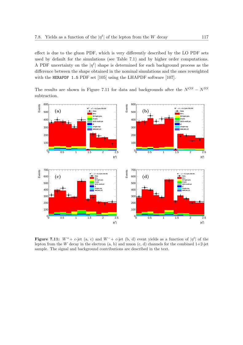
7.8. Yields as a function of the |η`| of the lepton from the W decay 117
effect is due to the gluon PDF, which is very differently described by the LO PDF sets
used by default for the simulations (see Table 7.1) and by higher order computations.
A PDF uncertainty on the |η`| shape is determined for each background process as the
difference between the shape obtained in the nominal simulations and the ones reweighted
with the HERAPDF 1.5 PDF set [105] using the LHAPDF software [107].
The results are shown in Figure 7.11 for data and backgrounds after the NOS − NSS
subtraction.
|eη|
0 0.5 1 1.5 2 2.5
Eve
nts
0
100
200
300
400
500
600 +1-2 jets OS-SSν+ e→+W
Data
W+c
W+light-jets
Z+jets
QCD multi-jet
ttsingle-top
WW,WZ,ZZ
(a)
|eη|
0 0.5 1 1.5 2 2.5
Eve
nts
0
100
200
300
400
500
600 +1-2 jets OS-SSν- e→-W
Data
W+c
W+light-jets
Z+jets
QCD multi-jet
ttsingle-top
WW,WZ,ZZ
(b)
|µη|
0 0.5 1 1.5 2 2.5
Eve
nts
0
100
200
300
400
500
600
700 +1-2 jets OS-SSν+µ →+W
DataW+cW+light-jetsZ+jetsQCD multi-jet
ttsingle-topWW,WZ,ZZ
(c)
|µη|
0 0.5 1 1.5 2 2.5
Eve
nts
0
100
200
300
400
500
600
700 +1-2 jets OS-SSν-µ →-W
DataW+cW+light-jetsZ+jetsQCD multi-jet
ttsingle-topWW,WZ,ZZ
(d)
Figure 7.11: W++ c-jet (a, c) and W−+ c-jet (b, d) event yields as a function of |η`| of thelepton from the W decay in the electron (a, b) and muon (c, d) channels for the combined 1+2-jetsample. The signal and background contributions are described in the text.

118 Chapter 7. Measurement of the W+ c-jet production cross section
7.9 Cross section determination
The cross section is measured in a fiducial phase space region (see Table 7.14) with cuts
following the ones applied for the selection of the W+ c-jet data sample in order to avoid
a model-dependent phase space extrapolation of the experimental result. A small phase
space extrapolation from the kinematic regions defined by the different electron and muon
selection cuts to a common phase space is performed to facilitate the comparison of the
results in the two leptonic channels and to combine them to a fiducial cross section mea-
surement for events with a W → `ν decay. This phase space extrapolation does not
introduce a significant systematic error in the cross section measurement since the rele-
vant kinematic variables are found to be well described in simulation.
Table 7.14: Fiducial phase space region for the W+ c-jet cross section measurement. The fiducialcuts on the soft muon are applied only for the W+ c-jet cross section measured for events with ac→ µ+X decay.
W → eν/W → µν selection
W → τν → e/µννν decays ExcludedLepton momentum pT > 20 GeVLepton pseudo-rapidity |η| <2.5Neutrino pT > 25 GeVW transverse mass mW
T > 40 GeV
Jet selection
Jet momentum pT > 25 GeVJet pseudo-rapidity |η| < 2.5Jet multiplicity 1 ≤ njet ≤ 2
c-jet selection
c-hadron momentum pT > 5 GeVc-hadron-jet matching ∆R(hadron, jet) < 0.3c-jet multiplicity nc-jet = 1
Soft muon (from c-hadron-decay)
Soft muon momentum pT > 4 GeVSoft muon pseudo-rapidity |η| <2.5Soft muon-jet matching ∆R(soft µ, jet) < 0.5
The fiducial cross section for the production of a leptonically decaying W boson in associ-
ation with a charm hadron jet, with the c-hadron decaying semileptonically into a muon,
is determined using the equation
σfidW+ c-jet(c→µ) ×BR(W → `ν) =NOS−SSdata −NOS−SS
bkg
Ufid ·∫Ldt
, (7.20)
where NOS−SSdata and NOS−SS
bkg are the signal and background yields after the NOS −NSS
subtraction, respectively, Ufid is the signal selection efficiency in the fiducial phase space

7.9. Cross section determination 119
region and∫Ldt the integrated luminosity. The selection efficiency is separately evaluated
for events with exactly one and exactly two jets and for the two leptonic channels. The
fiducial cross section for W+ c-jet events, without requiring a semimuonic decay of the
c-hadron, is evaluated as
σfidW+ c-jet ×BR(W → `ν) =σfidW+ c-jet(c→µ) ×BR(W → `ν)
Bfid(7.21)
where Bfid corrects for the average branching ratio of the semileptonic decays of c-hadrons
and for the efficiency on signal of the fiducial cuts applied to the soft muon (see Table 7.14).
The cross section is also measured separately for W++ c-jet and W−+ c-jet productions
and as a function of |η`| of the lepton from the W decay.
7.9.1 Determination of the selection efficiency
The signal selection efficiency is defined as
Ufid =NW+ c-jet(c→µ),OS−SSMC,reco
NW+ c-jet(c→µ),OS−SSMC,truth
, (7.22)
and determined in W + c simulated events.
The numerator of Eq. 7.22 is evaluated at reconstruction level, i.e. after full simulation of
the detector response, using the analysis selection (see Section 7.4). Several corrections are
applied to the simulated events to ensure a realistic simulation of the data taking condi-
tions and of the performance of the detector: the pile-up conditions, the distribution of the
z coordinate of the primary interaction vertex, the energy scale and resolution of leptons,
jets and EmissT , the lepton trigger and reconstruction efficiencies and the tagging efficiency
and the mistag rate of the Soft Muon Tagger are corrected in Monte Carlo to match the
data measurements. A further correction is applied to the description of the charm quark
fragmentation and to the modelling of the decays of the charm hadrons (see Section 7.9.3).
In the denominator of Eq. 7.22 Monte Carlo W+c events in the fiducial phase space region
of Table 7.14 at generator level are selected. The truth jets are reconstructed using the
anti-kT algorithm with a distance parameter of R = 0.4 for stable particles. A truth jet is
identified as a c-jet if a c-hadron with pT > 5 GeV is found within ∆R = 0.3 of the jet axis.
c-hadrons originating from b-hadron decays are excluded. The potential bias introduced
by this procedure has been studied using quarks instead of hadrons and changing the pT
and ∆R cuts. These variations lead only to per-mill level differences.
The momenta of the W -leptons are evaluated before the emission of final state radiation
photons. Three corrections are applied at generator level: the pile-up conditions and the
distribution of the z coordinate of the primary interaction vertex are reweighted to repro-
duce the data, and the charm quark fragmentation modelling and the description of the

120 Chapter 7. Measurement of the W+ c-jet production cross section
semimuonic decays of c-hadrons are corrected as described in Section 7.9.3.
The NOS − NSS subtraction is applied at generator level as well in order to correct for
the small fraction of events, about 1%, which are either produced by double parton inter-
actions or in which the soft muon inside the c-hadron jet is not produced by the c-hadron.
W → τν → e/µννν decays are an irreducible background on the order of 2% for the
measurement which is corrected for by the selection efficiency by keeping these events in
the numerator, at reconstruction level, but removing them from the denominator.
The results for the selection efficiency are shown in Table 7.15.
7.9.2 Determination of the extrapolation factor
Bfid is the extrapolation factor from the σfidW+ c-jet(c→µ) to the σfidW+ c-jet cross section and
it is evaluated from Monte Carlo signal events at generator level as
Bfid =NW+ c-jet(c→µ),OS−SSMC,truth
NW+ c-jet,OS−SSMC,truth
. (7.23)
The numerator is identical with the denominator of Ufid, while for the denominator the
requirement of a soft muon associated with the c-jet is dropped. The corrections used at
generator level for the determination of Ufid (see Section 7.9.1) are applied also in this
case. Bfid is expected to be identical for the two lepton channels. Using Equations 7.22
and 7.23,
Ufid · Bfid =NW+ c-jet(c→µ),OS−SSMC,reco
NW+ c-jet,OS−SSMC,truth
(7.24)
and the W+ c-jet cross section can be directly determined from the event yields with the
equation
σfidW+ c-jet ×BR(W → `ν) =NOS−SSdata −NOS−SS
bkg
Ufid · Bfid ·∫Ldt
. (7.25)
The results for Bfid and Ufid · Bfid are shown in Table 7.15.
7.9.3 c-hadron fragmentation and decay
The description of the c quark fragmentation and of the semileptonic decays of c-hadrons
in Monte Carlo simulations is essential to the correct description of the properties of the
c-jets and of the soft muons. For this reason the following parameters of the simulation
have been tuned to the most recent measurements:
the c quark fragmentation fractions for D0, D±, D±s and Λ±c hadrons,

7.9. Cross section determination 121
Table 7.15: Correction factors Ufid and Bfid and their product for the electron and muonchannels. The uncertainties are statistical only.
Channel Jet multiplicity Ufid Bfid Ufid · Bfid
Electron1-jet 0.3605± 0.0037 0.0486± 0.0004 0.0175± 0.00022-jet 0.4315± 0.0070 0.0514± 0.0007 0.0222± 0.00051+2-jet 0.3767± 0.0033 0.0492± 0.0003 0.0185± 0.0002
Muon1-jet 0.3687± 0.0037 0.0481± 0.0004 0.0177± 0.00022-jet 0.4102± 0.0070 0.0519± 0.0007 0.0213± 0.00051+2-jet 0.3784± 0.0033 0.0489± 0.0003 0.0185± 0.0002
the c quark fragmentation function,
the semimuonic decay branching ratios of the different c-hadron species and
the soft muon momentum (p∗) spectrum in the rest frame of the c-hadron.
The reweighting is applied both at reconstruction and at generator level.
The c quark fragmentation fractions are the fractions of different c-hadron species pro-
duced in the hadronization of the c quark. They are reweighted in the W +c signal sample
according to the most recent average of results obtained at e+e− and ep colliders [121]
(see Table 7.16). The uncertainty in these measurements is included in the systematic
uncertainty of the W+ c-jet cross section.
Table 7.16: Fragmentation fractions of the c quark from HERA [121]
D0 D± D±s Λ±cFraction 0.5643±0.0151 0.2256±0.0077 0.0797±0.0045 0.1080±0.0091
The c quark fragmentation function describes the fraction of transverse momentum of the
c-jet carried by the first c-hadron in the jet. No correction is applied to the fragmentation
function used by Pythia [43]. A systematic uncertainty arises from the comparison of the
Pythia and Herwig [45] charm fragmentation description. The different fragmentation
function used by the two programs, which are both used for the parton shower simulation
together with the Alpgen generator [47], leads to different predictions for thepc−hadronT
pc-jetT
distribution shown in Figure 7.12 for D± and Λ±c .
The branching ratios of the semimuonic decays of the different c-hadrons species into
muons are corrected for according to the measurements in [25] (see Table 7.17). For
D0, D± and Λ±c the more precise measurements of the decays into electrons are used
assuming lepton universality. For D±s , the semimuonic decay branching ratio includes
τ → µνν decays. To evaluate the branching ratios of Ω0c , Ξ0
c , Ξ±c decays into muons the
Λ±c → µ+X semimuonic branching ratio is scaled with the lifetime ratio:

122 Chapter 7. Measurement of the W+ c-jet production cross section
T
truth~jet/p
Thadronp
0 0.1 0.2 0.3 0.4 0.5 0.6 0.7 0.8 0.9 1
Arb
itrar
y un
its
0
0.01
0.02
0.03
0.04
0.05
0.06
0.07PythiaHerwig
±D
Simulation
(a)
T
truth~jet/p
Thadronp
0 0.1 0.2 0.3 0.4 0.5 0.6 0.7 0.8 0.9 1
Arb
itrar
y un
its
0
0.01
0.02
0.03
0.04
0.05
0.06
0.07
PythiaHerwig
c±Λ
Simulation
(b)
Figure 7.12: Normalised distributions ofpc−hadronT
pc-jetT
as predicted by Pythia (black) and Herwig
(red) for D± mesons (a) and Λ±c barions (b).
BRΩ0c ,Ξ
0c ,Ξ±c
=τΩ0
c ,Ξ0c ,Ξ±c
τΛ±c
· BRΛ±c. (7.26)
Table 7.17: Branching ratios of the c-hadron decays into muons [25]
D0 D± D±s Λ±c Ω0c Ξ0
c Ξ±cBR[%] 6.49±0.11 16.07±0.30 7.4±0.4 4.5±1.7 2.5±1.0 9.9±3.8 1.6±0.6
The distribution of the momentum p∗ of the soft muons from the c-hadron decay in the
rest frame of the c-hadron has direct impact on the efficiency of the Soft Muon Tagger.
Different Monte Carlo generators make different predictions, as shown in Figure 7.13 for
D± and Λ±c decays. The Alpgen+Pythia Monte Carlo sample is reweighted to fit the
predictions by EvtGen [52] which is expected to give the best description of the data.
The difference between EvtGen and Pythia is used as systematic uncertainty.
[MeV]*
p
0 100 200 300 400 500 600 700 800 900 1000
Arb
itrar
y un
its
0
0.02
0.04
0.06
0.08
0.1
0.12
0.14 PythiaHerwigEvtGen
±DSimulation
(a)
[MeV]*
p
0 100 200 300 400 500 600 700 800 900 1000
Arb
itrar
y un
its
0
0.02
0.04
0.06
0.08
0.1
0.12
0.14 PythiaHerwigEvtGen
c±Λ
Simulation
(b)
Figure 7.13: Normalised distributions of the momentum p∗ of the soft muons from decays ofc-hadrons D± (a) and Λ±
c (b) at rest, as predicted by Pythia (black), Herwig (red) and EvtGen(blue).
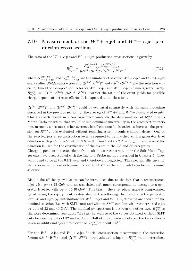
7.10. Measurement of the W++ c-jet and W−+ c-jet production cross sections 123
7.10 Measurement of the W++ c-jet and W−+ c-jet pro-
duction cross sections
The ratio of the W++ c-jet and W−+ c-jet production cross sections is given by
Rfid+/− =NOS−SSW++ c-jet
/NOS−SSW−+ c-jet
(Ufid · Bfid)+/(Ufid · Bfid)−, (7.27)
where NOS−SSW++ c-jet
and NOS−SSW−+ c-jet
are the numbers of selected W++ c-jet and W−+ c-jet
events after OS-SS subtraction and (Ufid · Bfid)+ and (Ufid · Bfid)− are the selection effi-
ciency times the extrapolation factor for W++ c-jet and W−+ c-jet channels, respectively.
Rcorr+/− = (Ufid · Bfid)+/(Ufid · Bfid)− correct the ratio of the event yields for possible
charge-dependent detector effects. It is expected to be close to 1.
(Ufid · Bfid)+ and (Ufid · Bfid)− could be evaluated separately with the same procedure
described in the previous section for the average of W+ + c and W−+ c simulated events.
This approach results in a too large uncertainty on the determination of Rcorr+/− due to
Monte Carlo statistics, that would be the dominant uncertainty in the cross section ratio
measurement since most other systematic effects cancel. In order to increase the preci-
sion on Rcorr+/−, it is evaluated without requiring a semimuonic c-hadron decay. One of
the selected jets at reconstruction level is required to be matched with a generator level
c-hadron with pT > 5 GeV within ∆R = 0.3 (so-called truth labelling). The charge of the
c-hadron is used for the classification of the events in the OS and SS categories.
Charge-dependent detector effects from soft muon reconstruction or the Soft Muon Tag-
ger cuts have been studied with the Tag-and-Probe method described in Chapter 5. They
were found to be at the 0.1% level and therefore are neglected. The selection efficiency for
the ratio measurement determined before the SMT is therefore valid also for the nominal
selection.
Bias in the efficiency evaluation can be introduced due to the fact that a reconstructed
c-jet with pT ≈ 25 GeV and an associated soft muon corresponds on average to a gen-
erator level jet with pT ≈ 35-40 GeV. This bias in the c-jet phase space is compensated
by adjusting the c-jet pT cut as described in the following. In Figure 7.14 the generator
level W and c-jet pT distributions for W++ c-jet and W−+ c-jet events are shown for the
nominal selection (i.e. with SMT cuts) and without SMT cuts but with reconstructed c-jet
pT cuts of 32 and 40 GeV. The nominal pT spectrum is between the other two. Rcorr+/− is
therefore determined (see Table 7.18) as the average of the values obtained without SMT
cuts for c-jet pT cuts of 32 and 40 GeV. Half of the difference between the two values is
taken as additional systematic error on Rcorr+/− of about 0.5%.
For the W++ c-jet and W−+ c-jet fiducial cross section measurements the correction
factors (Ufid · Bfid)+ and (Ufid · Bfid)− are evaluated using the Rcorr+/− value determined

124 Chapter 7. Measurement of the W+ c-jet production cross section
with the procedure described above using the equation
(Ufid · Bfid)+ =NW++ c-jet(c→µ),OS−SSMC,reco
NW++ c-jet,OS−SSMC,truth
=NW++ c-jet(c→µ),OS−SSMC,reco
NW++ c-jet,OS−SSMC,truth
·NW++ c-jet(c→µ),OS−SSMC,reco +N
W−+ c-jet(c→µ),OS−SSMC,reco
NW++ c-jet(c→µ),OS−SSMC,reco +N
W−+ c-jet(c→µ),OS−SSMC,reco
=NW++ c-jet(c→µ),OS−SSMC,reco +N
W−+ c-jet(c→µ),OS−SSMC,reco
NW++ c-jet,OS−SSMC,truth +N
W−+ c-jet(c→µ),OS−SSMC,reco · NW++ c-jet,OS−SS
MC,truth /NW++ c-jet(c→µ),OS−SSMC,reco
=NW++ c-jet(c→µ),OS−SSMC,reco +N
W−+ c-jet(c→µ),OS−SSMC,reco
NW++ c-jet,OS−SSMC,truth +NW−+ c-jet,OS−SS
MC,truth /Rcorr+/−
and similarly
(Ufid · Bfid)− =(N
W++ c-jet(c→µ),OS−SSMC,reco +N
W−+ c-jet(c→µ),OS−SSMC,reco )
Rcorr+/−NW++ c-jet,OS−SSMC,truth +NW−+ c-jet,OS−SS
MC,truth
.
Table 7.18: Correction factors (Ufid ·Bfid)+/(Ufid ·Bfid)− for the electron and the muon channel.The uncertainties are statistical only.
Channel 1-jet 2-jet 1+2-jet
Electron 0.999± 0.006 0.997± 0.009 0.998± 0.005
Muon 1.011± 0.005 0.986± 0.008 1.004± 0.004
7.11 Systematic uncertainties
Systematic uncertainties due to background estimation, detector effects and signal simu-
lation are taken into account.
7.11.1 Background estimation
The assessment of the uncertainties in the background contributions to W+ c-jet events
is discussed in Section 7.5 while the additional background uncertainties for W+ + c and
W−+ c event yields are evaluated as described in Section 7.7. The resulting uncertainties
in the measured yields are shown for the combination of the 1 and 2-jet samples separately
for W+ + c and W− + c events in Tables 7.19 and 7.20 for the electron and muon chan-
nel, respectively. The uncertainties in the OS/SS asymmetry and in the normalisation
of the background contributions are treated separately in the the electron channel due
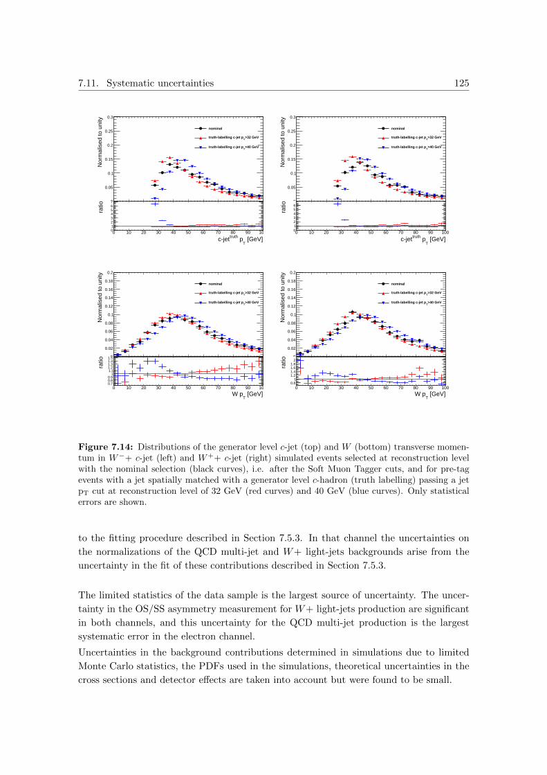
7.11. Systematic uncertainties 125
[GeV]T
ptruthc-jet
0 10 20 30 40 50 60 70 80 90 100
Nor
mal
ised
to u
nity
0
0.05
0.1
0.15
0.2
0.25
0.3
nominal
>32 GeVT
truth-labelling c-jet p
>40 GeVT
truth-labelling c-jet p
[GeV]T
ptruthc-jet0 10 20 30 40 50 60 70 80 90 100
ratio
01234567
[GeV]T
ptruthc-jet
0 10 20 30 40 50 60 70 80 90 100
Nor
mal
ised
to u
nity
0
0.05
0.1
0.15
0.2
0.25
0.3
nominal
>32 GeVT
truth-labelling c-jet p
>40 GeVT
truth-labelling c-jet p
[GeV]T
ptruthc-jet0 10 20 30 40 50 60 70 80 90 100
ratio
0123456
[GeV]T
W p
0 10 20 30 40 50 60 70 80 90 100
Nor
mal
ised
to u
nity
0
0.02
0.04
0.06
0.08
0.1
0.12
0.14
0.16
0.18
0.2
nominal
>32 GeVT
truth-labelling c-jet p
>40 GeVT
truth-labelling c-jet p
[GeV]T
W p0 10 20 30 40 50 60 70 80 90 100
ratio
0.70.80.9
11.11.21.31.41.5
[GeV]T
W p
0 10 20 30 40 50 60 70 80 90 100
Nor
mal
ised
to u
nity
0
0.02
0.04
0.06
0.08
0.1
0.12
0.14
0.16
0.18
0.2
nominal
>32 GeVT
truth-labelling c-jet p
>40 GeVT
truth-labelling c-jet p
[GeV]T
W p0 10 20 30 40 50 60 70 80 90 100
ratio
0.81
1.21.41.61.8
2
Figure 7.14: Distributions of the generator level c-jet (top) and W (bottom) transverse momen-tum in W−+ c-jet (left) and W++ c-jet (right) simulated events selected at reconstruction levelwith the nominal selection (black curves), i.e. after the Soft Muon Tagger cuts, and for pre-tagevents with a jet spatially matched with a generator level c-hadron (truth labelling) passing a jetpT cut at reconstruction level of 32 GeV (red curves) and 40 GeV (blue curves). Only statisticalerrors are shown.
to the fitting procedure described in Section 7.5.3. In that channel the uncertainties on
the normalizations of the QCD multi-jet and W+ light-jets backgrounds arise from the
uncertainty in the fit of these contributions described in Section 7.5.3.
The limited statistics of the data sample is the largest source of uncertainty. The uncer-
tainty in the OS/SS asymmetry measurement for W+ light-jets production are significant
in both channels, and this uncertainty for the QCD multi-jet production is the largest
systematic error in the electron channel.
Uncertainties in the background contributions determined in simulations due to limited
Monte Carlo statistics, the PDFs used in the simulations, theoretical uncertainties in the
cross sections and detector effects are taken into account but were found to be small.

126 Chapter 7. Measurement of the W+ c-jet production cross section
For the differential cross section measurement as a function of |η`| of the lepton from the
W decay additional uncertainties in the |η`| dependence of the backgrounds have to be
taken into account (see Section 7.8).
Table 7.19: Uncertainties in the W++ c-jet and W−+ c-jet yields N+ and N− and their ratioRW++ c-jet/W−+ c-jet in the electron channel for events with one or two selected jets. Otherbackgrounds are tt, single-top, diboson and Z+ jets events.
Uncertainty [%] N+ N− RW++ c-jet/W−+ c-jet
Data statistics 4 3.3 5.2
QCD (or W+ light-jets) background normalisation 1.2 0.6 0.6QCD background asymmetry 3.5 2.9 0.5W+ light-jets background asymmetry 2.7 1.6 1QCD background ratio 0.1 0.1 0.2W+ light-jets background ratio 0.2 0.1 0.4Other backgrounds normalisations 0.3 0.2 0.1Other backgrounds asymmetries 0.5 0.4 0.1Other backgrounds ratios 0 0 0.1
Total 6.2 4.8 5.4
Table 7.20: Uncertainties in the W++ c-jet and W−+ c-jet yields N+ and N− and their ra-tio RW++ c-jet/W−+ c-jet in the muon channel for events with one or two selected jets. Otherbackgrounds are tt, single-top, and diboson events.
Uncertainty [%] N+ N− RW++ c-jet/W−+ c-jet
Data statistics 3.5 3.0 4.6
QCD background normalisation 0.7 0.6 0.1W+ light-jets background normalisation 2.0 1.2 0.8Z+ jets background normalisation 0.6 0.5 0.1QCD background ratio 0.1 0.1 0.1W+ light-jets background ratio 0.7 0.6 1.3Z+ jets background ratio 0.2 0.1 0.3Other backgrounds normalisations 0.6 0.5 0.2Other backgrounds ratio 0 0 0.1
Total 4.2 3.4 4.9
7.11.2 Detector effects
The impact of the uncertainties in reconstruction efficiencies and in energy/momentum
scales and resolutions is evaluated by varying these parameters within their measurement
errors. Uncertainties in the lepton trigger, reconstruction and isolation efficiencies, the
lepton energy/momentum scales and resolutions, the SMT efficiency and mistag rate, the
jet energy scale (see [73]), the jet energy resolution (see [122]) and the EmissT determina-
tion are taken into account. The uncertainty in the jet energy resolution is determined as

7.11. Systematic uncertainties 127
the average of the uncertainties in the two leptonic channels to reduce the impact of the
limited Monte Carlo statistics on its estimation. All corrections applied to particle and
jet momenta are propagated to EmissT measurement, therefore most Emiss
T uncertainties are
already included in the previously discussed uncertainties. Uncertainties in the energy
scale and resolution due to the soft EmissT contributions (see Section 4.6) evaluated in [80]
are additionally taken into account.
The results are presented in Table 7.21 and Table 7.22 for the electron and muon channels,
respectively. Uncertainties from the determination of the lepton reconstruction efficiency
and of the jet energy scale are the by far largest contributions.
Table 7.21: Systematic uncertainties due to detector effects in the electron channel
Uncertainty [%] 1-jet 2-jet 1+2-jet
Electron Charge Flip 0.3 < 0.1 0.2Electron efficiency 1.9 1.9 1.9Electron energy scale 0.9 0.3 0.8Electron energy resolution 0.2 < 0.1 0.1Muon efficiency 1.2 1.1 1.1Muon energy scale < 0.1 < 0.1 < 0.1Muon energy resolution < 0.1 < 0.1 < 0.1SMT efficiency 0.5 0.5 0.5SMT fake rate 0.2 0.4 0.3Jet energy Resolution 0.5 < 0.1 0.3Jet Energy Scale 1.5 7.5 3.1Soft Emiss
T resolution 0.2 0.6 < 0.1Soft Emiss
T scale 0.6 0.6 0.6
Total 3.0 7.9 4.0
Table 7.22: Systematic uncertainties due to detector effects in the muon channel
Uncertainty [%] 1-jet 2-jet 1+2-jet
Muon efficiency 2.8 2.7 2.8Muon energy scale 0.8 0.7 0.8Muon energy resolution < 0.1 0.4 0.1SMT efficiency 0.5 0.5 0.5SMT fake rate 0.1 < 0.1 0.1Jet energy resolution 0.5 < 0.1 0.3Jet energy scale 1.5 6.4 2.7Soft Emiss
T resolution < 0.1 0.3 < 0.1Soft Emiss
T scale 0.2 0.6 0.1
Total 3.4 7.0 4.0

128 Chapter 7. Measurement of the W+ c-jet production cross section
7.11.3 Uncertainties in W + c signal modelling
The Monte Carlo description of the fragmentation and semileptonic decays of the c-hadrons
is a significant source of systematic error for the W+ c-jet cross section measurement which
is assessed as discussed in Section 7.9.3.
The uncertainty due to non-perturbative effects in the simulation of parton showers is
estimated by comparing the selection efficiency determined using Alpgen Monte Carlo
simulations of W + c production showered alternatively with Pythia and Herwig pro-
grams. Effects estimated in the two leptonic channels are averaged to reduce the impact
of the limited Monte Carlo statistics.
Another source of uncertainty is the modelling of the kinematics of the W → lν decay.
The lepton pT, EmissT and mW
T distributions agree very well between data and simulations,
therefore no additional systematic uncertainties are assigned to them.
Uncertainties in the selection efficiency due to the PDFs used in the simulations have
been evaluated by reweighting the simulated W +c events for different PDF sets using the
LHAPDF software [107]. The impact of this effect is slightly higher in the electron than in
the muon channel because of the different selection kinematic cuts. The biggest difference
in the selection efficiency is between the nominal cteq6ll PDF set and the HERAPDF 1.5
set which is therefore used as the uncertainty due to the PDF description in the simulation.
The results are shown in Table 7.23 for the electron channel and in Table 7.24 for the
muon channel.
Table 7.23: Systematic uncertainties due to Monte Carlo modelling in the electron channel
1-jet 2-jet 1+2-jet
Uncertainty [%] U U ×B U U ×B U U ×BD0 fraction < 0.1 0.7 < 0.1 0.6 < 0.1 0.7D+ fraction < 0.1 1.3 < 0.1 1.2 < 0.1 1.3Ds fraction < 0.1 < 0.1 < 0.1 0.1 < 0.1 < 0.1Baryon fraction < 0.1 1.4 0.3 1.1 0.1 1.3Fragmentation function 1.6 0.3 1.1 0.6 1.5 0.4Non-perturbative 0.8 1.7 6.5 4.6 1.0 0.3D0 decay BR < 0.1 0.7 < 0.1 0.7 < 0.1 0.7D+ decay BR < 0.1 0.8 < 0.1 0.8 < 0.1 0.8Ds decay BR < 0.1 0.4 < 0.1 0.4 < 0.1 0.4Baryon decay BR < 0.1 2.1 0.3 2.3 0.1 2.2p∗ 1.4 1.6 1.3 1.3 1.4 1.5PDF 0.9 1.7 0.3 1.2 0.8 1.7
Total 2.4 4.3 6.7 5.9 2.4 3.9

7.12. W+ c-jet fiducial cross section results 129
Table 7.24: Systematic uncertainties due to Monte Carlo modelling in the muon channel
1-jet 2-jet 1+2-jet
Uncertainty [%] U U ×B U U ×B U U ×BD0 fraction < 0.1 0.3 < 0.1 0.3 < 0.1 0.3D+ fraction < 0.1 1.0 < 0.1 1.0 < 0.1 1.0Ds fraction < 0.1 < 0.1 0.1 0.2 < 0.1 0.1Baryon fraction < 0.1 1.3 0.3 0.9 < 0.1 1.2Fragmentation function 1.7 0.7 1.4 0.7 1.7 0.7Non-perturbative 0.8 1.7 6.5 4.6 1.0 0.3D0 decay BR < 0.1 0.7 < 0.1 0.8 < 0.1 0.7D+ decay BR < 0.1 0.8 < 0.1 0.8 < 0.1 0.8Ds decay BR < 0.1 0.4 < 0.1 0.3 < 0.1 0.4Baryon decay BR < 0.1 2.0 0.3 2.5 0.1 2.1p∗ 1.3 1.5 1.4 0.6 1.4 1.3PDF 0.3 0.5 0.3 0.4 0.3 0.5
Total 2.3 3.7 6.8 5.6 2.4 3.3
7.12 W+ c-jet fiducial cross section results
The fiducial cross section results for a leptonically decaying W boson produced in associa-
tion with one c-jet are shown in Table 7.25 separately for the electron and muon channels
and for the W++ c-jet, W−+ c-jet productions. Results are given separately for events
with exactly one jet and exactly two jets. The result for the combination of the jet cat-
egories (1+2-jet) is not the direct sum of the two individual cross sections, since for its
determination the background estimation and the systematic uncertainty assessment are
performed directly in the combined sample.
The cross section measured in the muon channel is higher than the one in the electron
channel with a significance of less than 2σ (see Table 7.26) when taking into account the
correlation between the systematic uncertainties in the two leptonic channels. The results
obtained in the electron and muon channels are therefore in agreement and can be com-
bined as discussed in Section 7.13.
The results for the ratio of the W++ c-jet and W−+ c-jet production cross sections in the
fiducial phase space of the measurement are given in Table 7.27.
A breakdown of the uncertainties for the σfidW+ c-jet×BR(W → `ν) measurement is shown
in Table 7.28 for the two leptonic channels. The results for the fiducial cross section
measurement as a function of |η`| of the lepton from the W decay are given in Section 7.13.

130 Chapter 7. Measurement of the W+ c-jet production cross section
Table 7.25: Fiducial cross sections measured in the electron and muon channels in the 1-jet and2-jet data sets and in their combination
Jet category Electron channel Muon channel
σfidW+ c-jet ×BR(W → `ν) [pb]
1-jet 47.97 ± 1.26(stat.) ± 3.39(syst.) 52.76 ± 1.25(stat.) ± 3.08(syst.)2-jet 11.85 ± 0.80(stat.) ± 1.65(syst.) 14.28 ± 0.84(stat.) ± 1.47(syst.)
1+2-jet 59.09 ± 1.53(stat.) ± 4.27(syst.) 66.98 ± 1.53(stat.) ± 3.96(syst.)
σfidW++ c-jet
×BR(W → `ν) [pb]
1-jet 22.33±0.93(stat)±1.66(syst) [pb] 25.86±0.92(stat)±1.58(syst) [pb]2-jet 5.77±0.59(stat)±0.86(syst) [pb] 6.38±0.63(stat)±0.67(syst) [pb]1+2-jet 27.81±1.13(stat)±2.14(syst) [pb] 32.14±1.13(stat)±2.01(syst) [pb]
σfidW−+ c-jet
×BR(W → `ν) [pb]
1-jet 25.62±0.86(stat)±1.77(syst) [pb] 26.87±0.84(stat)±1.60(syst) [pb]2-jet 6.08±0.54(stat)±0.80(syst) [pb] 7.90±0.55(stat)±0.84(syst) [pb]1+2-jet 31.28±1.04(stat)±2.17(syst) [pb] 34.87±1.04(stat)±2.05(syst) [pb]
Table 7.26: Difference between the measured fiducial cross section σfidW+ c-jet × BR(W → `ν) in
the electron and muon channels. The statistical and the total significance and the correlation ofthe systematic uncertainties between the two leptonic channels are given.
σfidW+ c-jet ×BR(W → `ν)
Jet channel Difference [pb] Stat. sign.[σ] Tot. sign.[σ] Correlation
1-jet -4.78 ± 1.78(stat.) ± 2.94(syst.) 2.7 1.4 0.512-jet -2.42 ± 1.16(stat.) ± 1.39(syst.) 2.1 1.3 0.47
1+2-jet -7.88 ± 2.16(stat.) ± 3.51(syst.) 3.6 1.9 0.56
Table 7.27: Rfid+/− measured in the electron and muon channels in the 1-jet and 2-jet data sets
and in their combination
Rfid+/−Jet category Electron channel Muon channel
1-jet 0.87 ± 0.05(stat.) ± 0.02(syst.) 0.96 ± 0.05(stat.) ± 0.03(syst.)2-jet 0.95 ± 0.13(stat.) ± 0.04(syst.) 0.81 ± 0.10(stat.) ± 0.03(syst.)
1+2-jet 0.89 ± 0.05(stat.) ± 0.02(syst.) 0.92 ± 0.04(stat.) ± 0.02(syst.)

7.13. Combination of the electron and muon channels 131
Table 7.28: Systematic uncertainties in the σfidW+ c-jet×BR(W → `ν) measurement in the electron
and muon channels. The semi-leptonic decay uncertainty includes uncertainties on the p∗ and onthe c-hadron semimuonic branching ratio.
Systematic uncertainty [%] Electron channel Muon channel1-jet 2-jet 1+2-jet 1-jet 2-jet 1+2-jet
Background yields 4.2 9.4 4.1 2.0 4.0 1.9Monte Carlo statistics 1.3 2.3 1.1 1.3 2.3 1.1Object reconstruction 3.0 7.9 4.0 3.4 7.0 4.0Semi-leptonic decay 2.9 2.9 2.9 2.8 2.8 2.7c-fragmentation 2.0 1.9 2.0 1.8 1.5 1.7Non-perturbative 1.7 4.6 0.3 1.7 4.6 0.3PDF 1.7 1.2 1.7 0.5 0.4 0.5Luminosity 1.8 1.8 1.8 1.8 1.8 1.8
Total 7.1 13.9 7.2 5.8 10.3 5.9
7.13 Combination of the electron and muon channels
The results in the electron and muon channels are combined, assuming lepton universality,
using an averaging technique developed by the HERA experiments [123, 124, 125].
Since the measurements in the electron and muon channels are statistically independent,
the average fiducial cross section σ can be obtained from the individual fiducial cross
sections σe and σµ by minimising
χ2(σ) =∑k=e,µ
(σk − σ)2
(∆statk )2
, (7.28)
where ∆statk are the statistical uncertainties for in the two channels and systematic errors
are disregarded. Taking into account the dependence of the measured cross sections on
the systematic uncertainties, which are estimated independently for the two channels, the
minimisation procedure can also be used to improve the estimates of these uncertainties.
Let j label a given systematic uncertainty which has a correlated influence on σe and
σµ and γe,µj be the estimated impact of this uncertainty on σe,µ assessed as described in
Section 7.11. Assuming that a refined estimation γ′e,µj of the uncertainty can be determined
and defining the relative correction to the estimation bj ≡ (γ′e,µj − γe,µj )/γe,µj , a modified
χ2 [124] can be written as
χ2(σ, b1...bN ) =∑k=e,µ
[σ −∑N
j=1 γkj σbj − σk]2
(∆statk )2 + (∆uncorr
k )2+
N∑j=1
b2j , (7.29)
with ∆uncorrk being the sum of the systematic uncertainties which have no correlated effects
on σe and σµ. The χ2 minimisation can be used to simultaneously determine the average
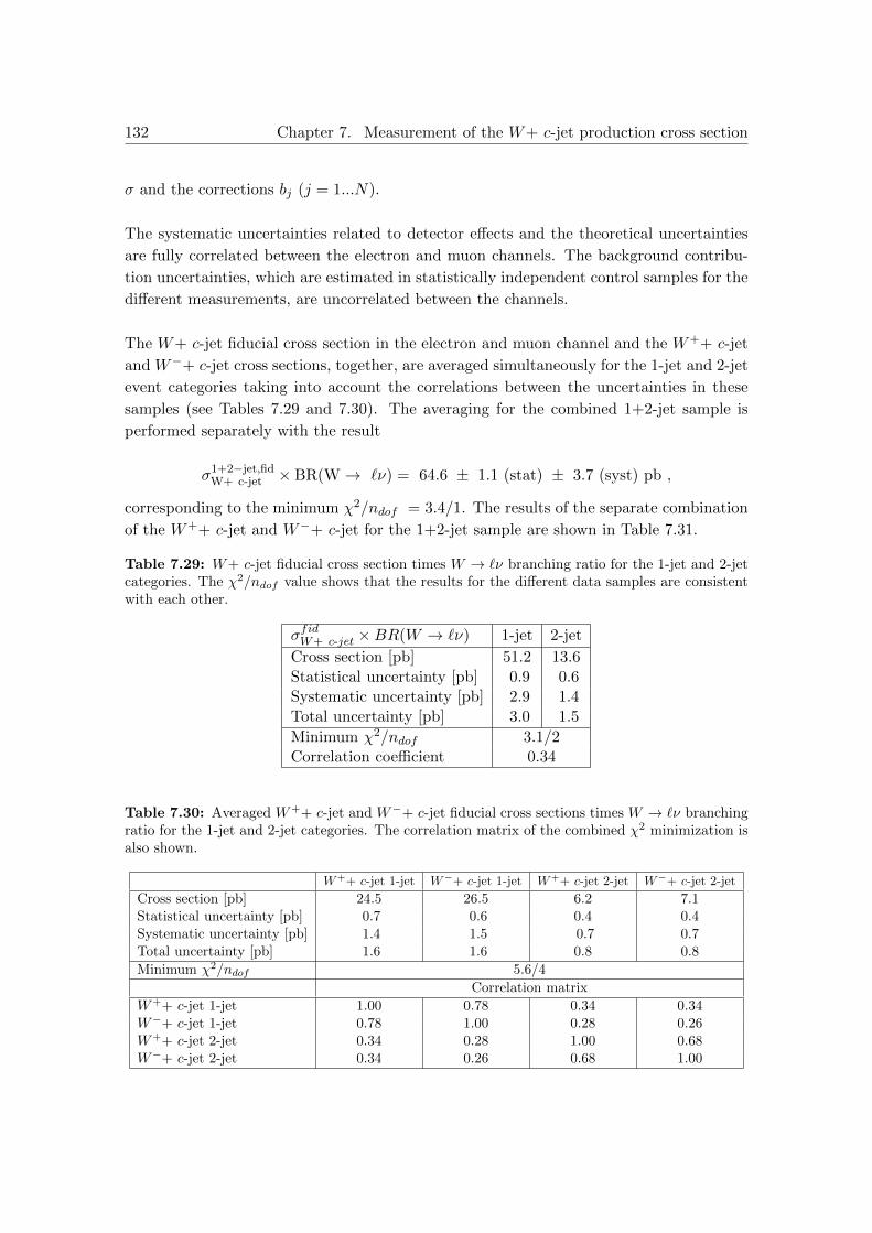
132 Chapter 7. Measurement of the W+ c-jet production cross section
σ and the corrections bj (j = 1...N).
The systematic uncertainties related to detector effects and the theoretical uncertainties
are fully correlated between the electron and muon channels. The background contribu-
tion uncertainties, which are estimated in statistically independent control samples for the
different measurements, are uncorrelated between the channels.
The W+ c-jet fiducial cross section in the electron and muon channel and the W++ c-jet
and W−+ c-jet cross sections, together, are averaged simultaneously for the 1-jet and 2-jet
event categories taking into account the correlations between the uncertainties in these
samples (see Tables 7.29 and 7.30). The averaging for the combined 1+2-jet sample is
performed separately with the result
σ1+2−jet,fidW+ c-jet × BR(W→ `ν) = 64.6 ± 1.1 (stat) ± 3.7 (syst) pb ,
corresponding to the minimum χ2/ndof = 3.4/1. The results of the separate combination
of the W++ c-jet and W−+ c-jet for the 1+2-jet sample are shown in Table 7.31.
Table 7.29: W+ c-jet fiducial cross section times W → `ν branching ratio for the 1-jet and 2-jetcategories. The χ2/ndof value shows that the results for the different data samples are consistentwith each other.
σfidW+ c-jet ×BR(W → `ν) 1-jet 2-jet
Cross section [pb] 51.2 13.6Statistical uncertainty [pb] 0.9 0.6Systematic uncertainty [pb] 2.9 1.4Total uncertainty [pb] 3.0 1.5
Minimum χ2/ndof 3.1/2Correlation coefficient 0.34
Table 7.30: Averaged W++ c-jet and W−+ c-jet fiducial cross sections times W → `ν branchingratio for the 1-jet and 2-jet categories. The correlation matrix of the combined χ2 minimization isalso shown.
W++ c-jet 1-jet W−+ c-jet 1-jet W++ c-jet 2-jet W−+ c-jet 2-jet
Cross section [pb] 24.5 26.5 6.2 7.1Statistical uncertainty [pb] 0.7 0.6 0.4 0.4Systematic uncertainty [pb] 1.4 1.5 0.7 0.7Total uncertainty [pb] 1.6 1.6 0.8 0.8
Minimum χ2/ndof 5.6/4
Correlation matrix
W++ c-jet 1-jet 1.00 0.78 0.34 0.34W−+ c-jet 1-jet 0.78 1.00 0.28 0.26W++ c-jet 2-jet 0.34 0.28 1.00 0.68W−+ c-jet 2-jet 0.34 0.26 0.68 1.00

7.14. Comparison with theoretical predictions 133
Table 7.31: Averaged W++ c-jet and W−+ c-jet fiducial cross sections times W → `ν branchingratio in the 1+2-jet category
W++ c-jet W−+ c-jet
Cross section [pb] 30.8 33.8Statistical uncertainty [pb] 0.8 0.7Systematic uncertainty [pb] 1.9 1.9Total uncertainty [pb] 2.0 2.1
Minimum χ2/ndof 3.5/2Correlation coefficient 0.81
The averaged ratio Rfid+/− of the fiducial W++ c-jet and W−+ c-jet cross sections for
the 1-jet and 2-jet categories are in Table 7.32 and the result for the combined 1+2-jet
category is
Rfid,1+2−jet+/− = 0.91 ± 0.03 (stat) ± 0.01 (syst) ,
with a minimum χ2/ndof = 0.2/1.
Table 7.32: Rfid+/− measurement in 1-jet and 2-jet categories
Rfid+/− 1-jet 2-jet
Ratio 0.92 0.87Statistical uncertainty 0.03 0.08Systematic uncertainty 0.02 0.03Total uncertainty 0.04 0.08
Fit χ2/ndof 2.3/2Correlation coefficient -0.02
Finally, the same combination is performed for the differential cross section measurements
in 11 |η`| bins. In order to increase the statistical precision, the 1 and 2 jets categories are
combined. TheW++ c-jet andW−+ c-jet measurements are simultaneously averaged with
a minimum χ2/ndof = 18.4/22. The latter fit has 20 degrees of freedom, 10 for W++ c-jet
and 10 for W−+ c-jet events, as in the bin corresponding to 1.37 < |η`| < 1.52 there is
only a cross section measurement in the muon channel. The results of the combination
are shown in Tables 7.33 and 7.34 and in Figure 7.15 in comparison with the individual
measurements for the two channels.
7.14 Comparison with theoretical predictions
The results presented in the last section are compared with leading order (LO) and next-
to-leading (NLO) order predictions obtained with the Alpgen [47] and aMC@NLO [50]
Monte Carlo generators, respectively. The Alpgen generator has been proved to pro-

134 Chapter 7. Measurement of the W+ c-jet production cross section
Table 7.33: W++ c-jet cross section times W → `ν branching ratio as function of the |η`| of thelepton from the W decay in the 1+2-jet sample. The |η`| bins are defined in Table 7.13.
|η`| bin 1 2 3 4 5 6 7 8 9 10 11
Cross section [pb] 3.80 3.56 3.54 3.40 3.13 4.31 1.93 2.33 1.86 1.67 2.04
Stat. error [pb] 0.26 0.24 0.23 0.25 0.25 0.28 0.26 0.23 0.22 0.22 0.29Syst. error [pb] 0.41 0.22 0.28 0.20 0.27 0.29 0.40 0.30 0.15 0.19 0.25Total. error [pb] 0.48 0.33 0.36 0.32 0.37 0.40 0.48 0.38 0.27 0.28 0.38
Table 7.34: W−+ c-jet cross section times W → `ν branching ratio as function of the |η`| of thelepton from the W decay in the 1+2-jet sample. The |η`| bins are defined in Table 7.13.
|η`| bin 1 2 3 4 5 6 7 8 9 10 11
Cross section [pb] 3.75 3.82 3.84 3.77 3.82 4.70 1.81 2.45 2.26 1.65 2.38
Stat. error [pb] 0.25 0.22 0.22 0.23 0.24 0.26 0.22 0.21 0.19 0.19 0.23Syst. error [pb] 0.25 0.28 0.23 0.21 0.21 0.30 0.40 0.19 0.20 0.17 0.28Total error [pb] 0.35 0.35 0.31 0.31 0.32 0.39 0.46 0.29 0.27 0.26 0.37
|lη|
0 0.5 1 1.5 2 2.5
| [pb
]η
/d|
fiduc
ial
+c-
jet
+Wσd
0
5
10
15
20
25
30
-1 Ldt = 4.6 fb∫=7 TeV, s (stat unc.)ν+ e→+W
Syst⊕Stat
(stat unc.)ν+µ →+W
Syst⊕Stat
(total unc.)ν+ l→+W
|lη|
0 0.5 1 1.5 2 2.5
| [pb
]η
/d|
fiduc
ial
+c-
jet
-Wσd
0
5
10
15
20
25
30
-1 Ldt = 4.6 fb∫=7 TeV, s (stat unc.)ν- e→-W
Syst⊕Stat
(stat unc.)ν-µ →-W
Syst⊕Stat
(total unc.)ν- l→-W
Figure 7.15: Differential cross sections for W++ c-jet (left) and W−+ c-jet (right) productionwith zero and one additional jet as a function of |η`| of the lepton ` = e, µ from the W decay forthe electron and muon channels and their combination.
vide a reliable description of the kinematics and jet multiplicities of W+ jets events [35].
aMC@NLO is a new NLO Monte Carlo generator which is used for the first time in
ATLAS in the context of W+ jets analyses for the W + c measurements in this thesis and
in [99].
The Alpgen predictions in this section are multiplied by a 1.195 scale factor to correct
the Alpgen W inclusive production cross section to the next-to-next-to-leading order

7.14. Comparison with theoretical predictions 135
(NNLO) calculation [33].
The comparison is performed for the different PDF sets introduced in Section 7.1. The
results are shown in Tables 7.35 and 7.36 for the aMC@NLO and Alpgen predictions,
respectively. The uncertainties on the predictions include Monte Carlo statistical errors
and the PDF uncertainties. Uncertainties due to renormalisation and factorization scales,
expected to be at 5% level (see [100]) are not taken into account. Figure 7.16 shows
the comparison of the measured W+ c-jet fiducial cross section with the aMC@NLO
and Alpgen predictions for events with zero or one additional jet. The measurement
agrees best with PDF predictions with small or no suppression of the s quark compared
to the d sea quark content as CT10 [106] and ATLAS WZ [34]. The predictions of the two
Monte Carlo generators are significantly different. The jet multiplicity of W+ c-jet events
in the fiducial phase space of the measurements is better described by Alpgen. The
ratios of the cross sections of W+ c-jet events with one additional jet and with no fur-
ther jet σfid,2−jetW+ c-jet/σfid,1−jetW+ c-jet predicted by Alpgen and aMC@NLO are 0.28 ± 0.04 and
0.41 ± 0.07, respectively, with the first in better agreement with the result obtained in
data 0.27 ± 0.03.
In order to be able to compare the results with the ones recently published by ATLAS
for the associated production of a W and a D meson [99] the experimental results are
compared with the aMC@NLO predictions from now on.
The Rfid+/− ratio between the W++ c-jet and W−+ c-jet fiducial cross sections is sensitive
to a possible asymmetry between the PDF of s and s quarks. It is expected to be smaller
than 1 even in absence of such asymmetry due to the contribution of Feynman diagrams
with a d or d quark in the initial state to the W+ c-jet production (see Figure 7.1). d
quarks are in the valence component of the proton, resulting in a higher contribution with
respect to d quarks. The measured value of Rfid+/− is compared with the aMC@NLO
predictions in Table 7.37 and in Figure 7.17. All the PDF sets used for the comparison
take into account small or no s/s asymmetry (see Section 7.1) and their predictions are
in agreement with the result in data within uncertainties.
In Figure 7.18 the fiducial cross section measured as a function of |η`| of the lepton from
the W decay for W++ c-jet and W−+ c-jet productions is compared with the predictions
for the 1+2-jet category. The cross section shape appears well described by all PDF set
apart from NNPDF 2.3coll which predicts a distribution flatter than measured in experi-
mental data.
The results shown in this thesis are therefore in favour of small or no s quark suppression
in the proton sea with respect to the contributions of lighter quarks, with uncertainties too
high to rule out PDF models taking into account higher strange suppression. This is in
agreement with the results obtained by ATLAS for the inclusive W and Z productions [34]

136 Chapter 7. Measurement of the W+ c-jet production cross section
and with the preliminary ATLAS results for the associated production of a W boson and
a D meson [99], both best consistent with no strange suppression. The preliminary results
published by CMS [100] for the W+ c-jet cross section are best in agreement with the CT10
set description, i.e. with small suppression. These results cannot be directly compared
with the ones presented in this thesis due to the different fiducial phase space of the ATLAS
and CMS measurements. The W++ c-jet/W−+ c-jet ratio measurements presented in this
thesis and in [99, 100] are limited by high statistical uncertainties and are therefore not
sensitive enough to prove or disprove a small asymmetry between the s and s quark PDFs.
The new results of this thesis and of [99, 100] provide new and more precise experimental
constraints for the s quark PDF determination.
Table 7.35: Comparison of the measured σfidW+ c-jet × BR(W → `ν) fiducial cross section with
the aMC@NLO predictions for different PDF sets
1-jet [pb] 2-jet [pb] 1+2-jet [pb]
Measured 51.2±3.0 13.6±1.5 64.6±3.9
CT10 [106] 40.4±4.8 16.4±1.9 56.8±6.6MSTW 2008 [103] 38.4±0.7 15.6±0.3 54.0±1.0NNPDF 2.3 [102] 36.9±1.3 15.1±0.5 51.9±1.8HERAPDF 1.5 [104, 105] 39.4±4.5 15.9±1.7 55.2±6.2ATLAS WZ [34] 44.7±3.8 18.0±1.4 62.7±5.2NNPDF 2.3coll [102] 49.4±5.3 19.7±2.0 69.1±7.3
Table 7.36: Comparison of the measured σfidW+ c-jet × BR(W → `ν) fiducial cross section with
the Alpgen predictions for different PDF sets
1-jet [pb] 2-jet [pb] 1+2-jet [pb]
Measured 51.2±3.0 13.6±1.5 64.6±3.9
CT10 [106] 48.4±5.6 13.7±1.4 62.1±7.0MSTW 2008 [103] 46.0±0.8 13.4±0.2 59.3±1.0NNPDF 2.3 [102] 43.9±1.6 12.8±0.5 56.7±2.1HERAPDF 1.5 [104, 105] 46.7±5.3 13.6±1.5 60.3±6.7ATLAS WZ [34] 53.4±4.5 15.0±1.2 68.4±5.6NNPDF 2.3coll [102] 59.5±7.1 17.7±2.4 77.2±9.4

7.14. Comparison with theoretical predictions 137
Table 7.37: Comparison of the measured ratio of the W++ c-jet and W−+ c-jet fiducial crosssections with the aMC@NLO predictions for different PDF sets
1-jet 2-jet 1+2-jet
Measured 0.92±0.04 0.87±0.08 0.91±0.03
CT10 [106] 0.92±0.01 0.90±0.02 0.92±0.01MSTW 2008 [103] 0.89±0.03 0.87±0.03 0.89±0.03NNPDF 2.3 [102] 0.90±0.02 0.88±0.02 0.89±0.02HERAPDF 1.5 [104, 105] 0.92±0.01 0.90±0.02 0.91±0.01ATLAS WZ [34] 0.93±0.01 0.91±0.02 0.92±0.01NNPDF 2.3coll [102] 0.93±0.03 0.91±0.03 0.92±0.02

138 Chapter 7. Measurement of the W+ c-jet production cross section
[pb]fiducialW+c-jetσ
0 10 20 30 40 50 60 70 80 90
-1 Ldt = 4.6 fb∫=7 TeV, s
, 1+2 jetsν l→W
Total uncertaintyStat. uncertainty
aMC@NLO+CT10aMC@NLO+MSTW08aMC@NLO+NNPDF23aMC@NLO+HERA15aMC@NLO+ATLASWZ
collaMC@NLO+NNPDF23
[pb]fiducialW+c-jetσ
0 10 20 30 40 50 60 70 80 90
-1 Ldt = 4.6 fb∫=7 TeV, s
, 1+2 jetsν l→W
Total uncertaintyStat. uncertainty
Alpgen+CT10Alpgen+MSTW08Alpgen+NNPDF23Alpgen+HERA15Alpgen+ATLASWZ
collAlpgen+NNPDF23
Figure 7.16: Fiducial cross section measurement for W+ c-jet production for events with zero andone additional jet compared with aMC@NLO (top) and Alpgen (bottom) predictions obtainedfor different PDF sets. The Alpgen leading order predictions shown in the plots are corrected bya scale factor 1.195 evaluated comparing the Alpgen W inclusive production cross section withNNLO calculations [33]. The uncertainties on the predictions include the statistical error and theuncertainties in the PDF description.

7.14. Comparison with theoretical predictions 139
+c-jet-Wfiducialσ/+c-jet+W
fiducialσ0 0.2 0.4 0.6 0.8 1
-1 Ldt = 4.6 fb∫=7 TeV, s
, 1+2 jetsν l→W
Total uncertaintyStat uncertainty
aMC@NLO+CT10aMC@NLO+MSTW08aMC@NLO+NNPDF23aMC@NLO+HERA15aMC@NLO+ATLASWZ
collaMC@NLO+NNPDF23
Figure 7.17: Ratio of the fiducial cross section measurements for W++ c-jet and W−+ c-jetproductions for events with zero and one additional jet compared with aMC@NLO predictionsobtained for different PDF sets. The uncertainties on the predictions include the statistical errorand the uncertainties in the PDF description.

140 Chapter 7. Measurement of the W+ c-jet production cross section
Figure 7.18: W++ c-jet (left) and W−+ c-jet (right) fiducial production cross sections for eventswith zero and one additional jet as a function of |η`| of the lepton form the W decay comparedto aMC@NLO predictions obtained for different PDF sets. The uncertainties on the predictionsinclude the statistical error and the uncertainties in the PDF description.

Conclusions
After three years of operation, the Large Hadron Collider (LHC) was shut down at the
beginning of 2013 for an upgrade in order to pursue a new ambitious physics program at
increased centre-of-mass energy of√
s = 13 TeV starting in 2015. During the last three
years the ATLAS detector at the LHC recorded more than 25 fb−1 of proton-proton col-
lision data at√
s = 7 and 8 TeV. With these data, the Standard Model predictions for
the new energy regime have been confirmed and a new particle with the properties of the
Standard Model Higgs boson has been discovered.
In this thesis, the cross sections for W boson production in association with charm and
bottom quark jets have been measured in proton-proton collisions at√
s = 7 TeV with
the ATLAS detector. The muon reconstruction efficiency of the ATLAS detector has been
determined from data, not only for the above cross section measurements but also for use
in all ATLAS analyses involving muons.
The measurement of W boson production in association with b quark jets is an important
test of perturbative QCD predictions. The process pp → W + bb + X is an important
background for many physics studies at the LHC such as the search for the Higgs boson
in decays H → W+W− and H → bb. The analysis presented in this thesis has been
performed by a small analysis team with a data set corresponding to an integrated lumi-
nosity of 35 pb−1 of proton-proton collisions at√
s = 7 TeV collected by ATLAS in 2010.
For the identification of the W bosons, their leptonic decays have been used. b-jets have
been identified by requiring a reconstructed b-hadron decay vertex belonging to the jet.
Data-driven methods have been used to evaluate the dominant background contributions
from tt, QCD multi-jet, W+ c-jets and W+ light-quark jets production. The main focus
of this work was on the development of the signal selection criteria, the determination of
the selection efficiency from data and the evaluation of the cross sections for W production
with a b-jet and zero or one additional jet together with their systematic uncertainties.
The measurement has been published in [1].
The results in a predefined kinematic fiducial region (see Table 6.4),
σfid(pp→W + b-jet) × BR(W → `ν) = 4.5 ± 1.3 ± 1.3 pb
141

and
σfid(pp→W + b-jet+ jet) × BR(W → `ν) = 5.7 ± 1.3 ± 1.4 pb ,
where BR(W → `ν) is the average leptonic branching ratio of the W boson, are consis-
tent with the next-to-leading order QCD predictions [95] for the fiducial cross sections,
2.9 ± 0.5 pb and 1.9+0.8−0.4 pb, respectively, in the two jet categories. The latter measurement
is 1.8 σ above the expectation. The subsequent measurement with 2011 ATLAS data [96]
agrees even better with the predictions.
The W+ c-jet cross section measurement presented in this thesis is of particular inter-
est because of the sensitivity of this process to the strange quark content of the proton,
which has large uncertainties, especially in the kinematic region of parton interactions at
the LHC. For exact flavour symmetry, up, down and strange quarks are expected to give
the same contributions to the proton sea quarks. But due to their higher mass and non-
perturbative QCD effects, the strange quark content of the proton is suppressed compared
to up and down by amounts depending on the analysis of the available data. The W+ c-jet
measurement has been performed by a very small analysis team with 4.6 fb−1 of proton-
proton collision data at√
s=7 TeV collected by ATLAS in 2011. W bosons have been
selected via their leptonic decays into electrons and muons. The associated c-jets have
been identified by the semileptonic decays of c-hadrons into muons. The uncertainties of
the contributions of QCD multi-jet, W+ light-quark jets and Z+ jets background events
to the W+ c-jet sample are minimised by using data driven background determination
techniques. A detailed study of the muon reconstruction and c-jet identification efficiencies
needed for measurements in this thesis has been performed. In addition, the focus of this
work has been on the optimization of the event selection criteria in the two leptonic decay
channels, on the determination of signal selection efficiency from data, on the evaluation
of the systematic uncertainties and on the evaluation of the cross sections for W boson
production in association with a c-jet and zero or one additional jet and their combination.
The combined result
σfid(pp→W + c-jet+ 0− 1 jet) × BR(W → `ν) = 64.6 ± 1.1 ± 3.7 pb ,
in a predefined kinematic fiducial region (see Table 7.14), is compared to the predictions
of the Alpgen [47] and aMC@NLO [50] Monte Carlo generators with different sets of
parton density functions (PDF). For Alpgen the best agreement is found using the CT10
PDF set [106], which involves a small suppression of the s quark density, with a predicted
cross section of 62.1 ± 7.0 pb. aMC@NLO gives the best prediction of 62.7 ± 5.2 pb for
the ATLAS WZ PDF set [34], which contains no s quark suppression. The results favour
models of the strange quark content of the proton with small or no suppression compared
to up and down sea quarks, but still does not exclude strange quark suppression.
142

The ratio of the fiducial cross sections for W++ c-jet and W−+ c-jet events with a maxi-
mum of one additional jet has been measured to be
Rfid+/− = 0.91 ± 0.03 ± 0.01
in agreement with the aMC@NLO prediction of 0.92 ± 0.01 for CT10 PDF set and similar
for the other PDF sets.
These results, together with other recent measurements by the CMS [98] and ATLAS [99]
experiments, are an important input for a more precise determination of the strange quark
density function in the proton.
143

144 Chapter 7. Measurement of the W+ c-jet production cross section
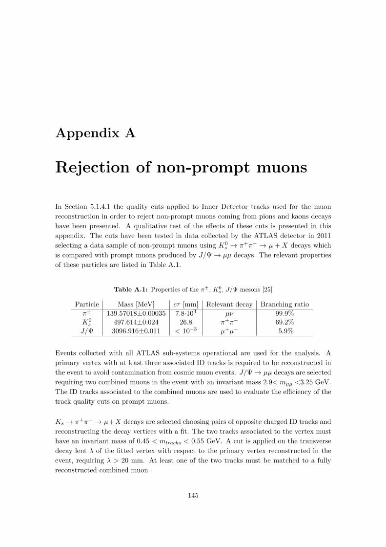
Appendix A
Rejection of non-prompt muons
In Section 5.1.4.1 the quality cuts applied to Inner Detector tracks used for the muon
reconstruction in order to reject non-prompt muons coming from pions and kaons decays
have been presented. A qualitative test of the effects of these cuts is presented in this
appendix. The cuts have been tested in data collected by the ATLAS detector in 2011
selecting a data sample of non-prompt muons using K0s → π+π− → µ + X decays which
is compared with prompt muons produced by J/Ψ→ µµ decays. The relevant properties
of these particles are listed in Table A.1.
Table A.1: Properties of the π±, K0s , J/Ψ mesons [25]
Particle Mass [MeV] cτ [mm] Relevant decay Branching ratio
π± 139.57018±0.00035 7.8·103 µν 99.9%K0s 497.614±0.024 26.8 π+π− 69.2%
J/Ψ 3096.916±0.011 < 10−3 µ+µ− 5.9%
Events collected with all ATLAS sub-systems operational are used for the analysis. A
primary vertex with at least three associated ID tracks is required to be reconstructed in
the event to avoid contamination from cosmic muon events. J/Ψ→ µµ decays are selected
requiring two combined muons in the event with an invariant mass 2.9< mµµ <3.25 GeV.
The ID tracks associated to the combined muons are used to evaluate the efficiency of the
track quality cuts on prompt muons.
Ks → π+π− → µ+X decays are selected choosing pairs of opposite charged ID tracks and
reconstructing the decay vertices with a fit. The two tracks associated to the vertex must
have an invariant mass of 0.45 < mtracks < 0.55 GeV. A cut is applied on the transverse
decay lent λ of the fitted vertex with respect to the primary vertex reconstructed in the
event, requiring λ > 20 mm. At least one of the two tracks must be matched to a fully
reconstructed combined muon.
145

146 Appendix A. Rejection of non-prompt muons
The efficiency of the track quality cuts of Table 5.3 has been measured to be about 60% and
98% for prompt and non-prompt muons respectively The latter measurement is compatible
with the one performed at higher energies on Z → µµ events presented in Section 5.1.5.

Appendix B
Muon reconstruction performance
in 2012 data
In 2012 more than 20 fb−1 of proton-proton collisions at√
s = 8 TeV have been recorded
by the ATLAS detector. In this section a brief overview of the performance of the ATLAS
Inner Detector (ID) and Muon Spectrometer (MS) in 2012 is given. The reconstruction
efficiency is measured in 16.9 fb−1 of 2012 data with the Tag-and-Probe method presented
in Chap. 5, with small changes in the selection due to the different data taking conditions.
A signal Powheg+Pythia Z → µµ Monte Carlo sample only has been used for this mea-
surement: for this reason the muon reconstruction has been determined using calorimeter
tagged probes which ensure a background contamination in data below 0.1%.
In Figure B.1 the ID reconstruction efficiency is shown. The efficiency of the quality cuts
of Table 5.3 is included in the measurement. The efficiency in data is measured to be about
98.5%, about 0.5% lower than the Monte Carlo prediction. The effects of the single cuts
are shown in Fig. B.2: the main source of this small discrepancy is the cut on the number
of hits in the B-layer (NB−layerhits > 0. This has been found to be due to dead modules which
are not taken into account in the simulation.
In Fig. B.3 a comparison of the muon reconstruction efficiency of the Staco and the Muid
chain for 2011 and 2012 data is shown for the combined (CB) muons and combined and
segment tagged (ST) muons. The only significant difference found is an increase of the
reconstruction efficiency for CB muons at η ≈ −1.1 as a consequence of the installation
of new tracking chambers in that region that improved the geometrical acceptance of the
detector. This gain is particularly relevant for the Staco CB reconstruction due to the
tight cuts applied by this algorithm. Small increases can be observed also in the forward
regions (|η| > 2).
A third algorithm chain, (Muons), has been introduced for the 2012 data set, combining
characteristics and algorithms of the two other chains. In Figure B.4 an overview of the
147

148 Appendix B. Muon reconstruction performance in 2012 data
-2.5 -2 -1.5 -1 -0.5 0 0.5 1 1.5 2 2.5
Effi
cien
cy
0.9
0.92
0.94
0.96
0.98
1
MC data
-1 Ldt =16.9 fb∫
2012 data, tracks
η-2.5 -2 -1.5 -1 -0.5 0 0.5 1 1.5 2 2.5
Dat
a/M
C
0.980.99
11.011.02
(a)
-3 -2 -1 0 1 2 3
Effi
cien
cy
0.9
0.92
0.94
0.96
0.98
1
MC data
-1 Ldt =16.9 fb∫
2012 data, tracks
φ-3 -2 -1 0 1 2 3
Dat
a/M
C
0.980.99
11.011.02
(b)
20 30 40 50 60 70 80 90 100
Effi
cien
cy
0.975
0.98
0.985
0.99
0.995
1
MC data
-1 Ldt =16.9 fb∫
2012 data, tracks
[GeV]T
p20 30 40 50 60 70 80 90 100
Dat
a/M
C
0.99
1
(c)
0 5 10 15 20 25 30 35 40 45 50
Effi
cien
cy
0.965
0.97
0.975
0.98
0.985
0.99
0.9951
1.005
MC data
-1 Ldt =16.9 fb∫
2012 data, tracks
>µ<0 5 10 15 20 25 30 35 40 45 50
Dat
a/M
C
0.990.995
11.005
(d)
Figure B.1: ID track reconstruction efficiency including the track quality criteria in Table 5.3measured as a function of η (a), φ (b), pT (c) and of the average number of collisions per bunchcrossing < µ > (d) for 2012 data and simulations. The bottom part of the plots shows the SF.Only statistical errors are shown.
performance this new chain is given, with a combined reconstruction efficiency in data of
about 98% well in agreement with the simulations.

149
-2.5 -2 -1.5 -1 -0.5 0 0.5 1 1.5 2 2.5
Effi
cien
cy
0.9
0.92
0.94
0.96
0.98
1
MC data
-1 Ldt =16.9 fb∫
2012 data, tracks
η-2.5 -2 -1.5 -1 -0.5 0 0.5 1 1.5 2 2.5
Dat
a/M
C
0.980.99
11.011.02
(a) Cut on the number ofPixel Detector hits
-2.5 -2 -1.5 -1 -0.5 0 0.5 1 1.5 2 2.5
Effi
cien
cy
0.9
0.92
0.94
0.96
0.98
1
MC data
-1 Ldt =16.9 fb∫
2012 data, tracks
η-2.5 -2 -1.5 -1 -0.5 0 0.5 1 1.5 2 2.5
Dat
a/M
C
0.980.99
11.011.02
(b) Cut on the number of SCT hits
-2.5 -2 -1.5 -1 -0.5 0 0.5 1 1.5 2 2.5
Effi
cien
cy
0.9
0.92
0.94
0.96
0.98
1
MC data
-1 Ldt =16.9 fb∫
2012 data, tracks
η-2.5 -2 -1.5 -1 -0.5 0 0.5 1 1.5 2 2.5
Dat
a/M
C
0.980.99
11.011.02
(c) Cut on the number of B-layer hits
-2.5 -2 -1.5 -1 -0.5 0 0.5 1 1.5 2 2.5
Effi
cien
cy
0.9
0.92
0.94
0.96
0.98
1
MC data
-1 Ldt =16.9 fb∫
2012 data, tracks
η-2.5 -2 -1.5 -1 -0.5 0 0.5 1 1.5 2 2.5
Dat
a/M
C
0.980.99
11.011.02
(d) Cut on the number of missing hits(holes) in the silicon detectors
-2.5 -2 -1.5 -1 -0.5 0 0.5 1 1.5 2 2.5
Effi
cien
cy
0.9
0.92
0.94
0.96
0.98
1
MC data
-1 Ldt =16.9 fb∫
2012 data, tracks
η-2.5 -2 -1.5 -1 -0.5 0 0.5 1 1.5 2 2.5
Dat
a/M
C
0.980.99
11.011.02
(e) Cut on the number of TRT hits
Figure B.2: ID track reconstruction efficiency measured as a function of η for 2012 data andMonte Carlo simulations after the different quality cuts in Table 5.3. The bottom part of the plotsshows the SF. Only statistical errors are shown.

150 Appendix B. Muon reconstruction performance in 2012 data
η
-2.5 -2 -1.5 -1 -0.5 0 0.5 1 1.5 2 2.5
Dat
a E
ffici
ency
0.5
0.6
0.7
0.8
0.9
1
20112012 2011-2012 data, Staco
(a)
η
-2.5 -2 -1.5 -1 -0.5 0 0.5 1 1.5 2 2.5
Dat
a E
ffici
ency
0.5
0.6
0.7
0.8
0.9
1
20112012 2011-2012 data, Muid
(b)
η
-2.5 -2 -1.5 -1 -0.5 0 0.5 1 1.5 2 2.5
Dat
a E
ffici
ency
0.65
0.7
0.75
0.8
0.85
0.9
0.95
1
20112012 2011-2012 data, Staco
(c)
η
-2.5 -2 -1.5 -1 -0.5 0 0.5 1 1.5 2 2.5
Dat
a E
ffici
ency
0.6
0.65
0.7
0.75
0.8
0.85
0.9
0.95
1
20112012 2011-2012 data, Muid
(d)
Figure B.3: Comparison of the muon reconstruction efficiency measured in 2011 (black circles)and 2012 (red triangles) data for the Staco (left plots) and Muid (right plots) combined (a, b) andcombined and segment tagged (c, d) muons.
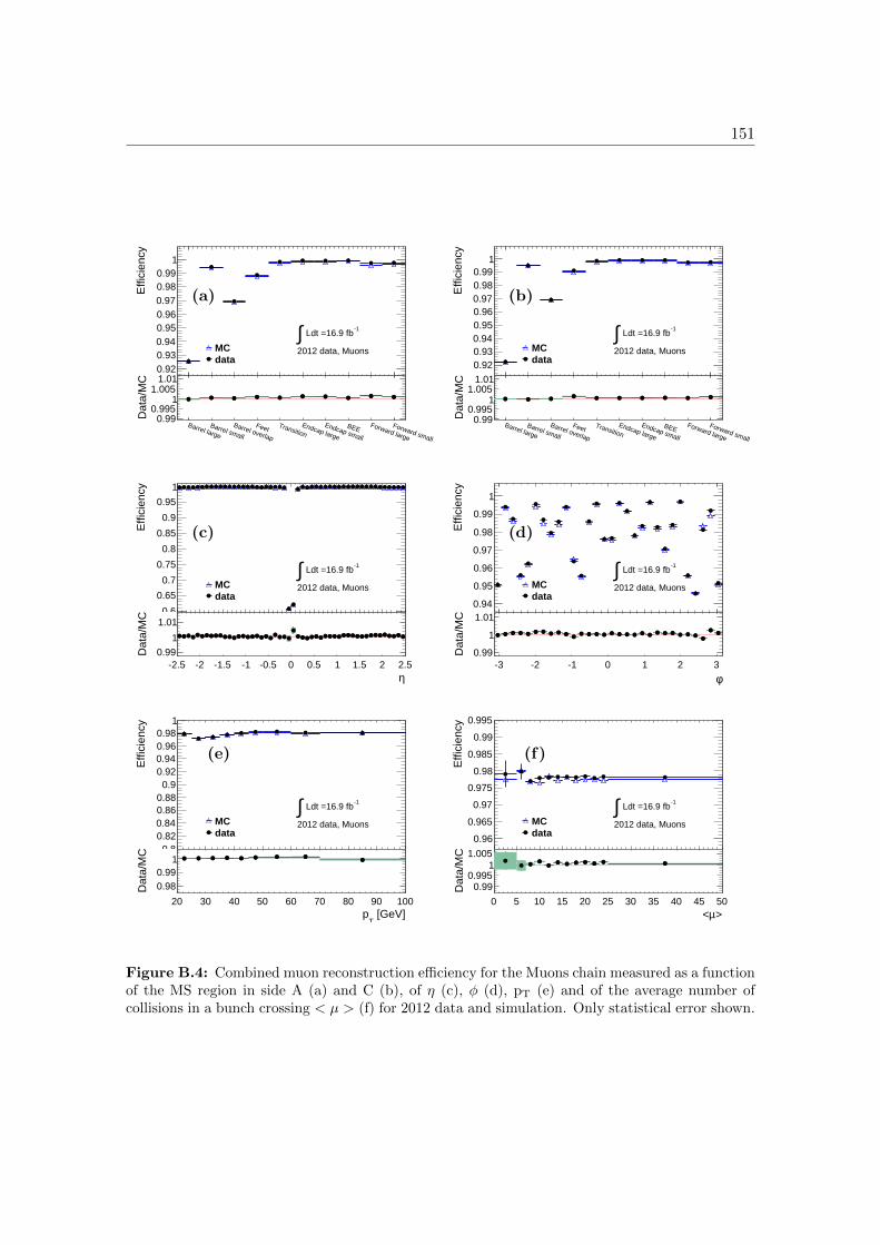
151
1 2 3 4 5 6 7 8 9 10
Effi
cien
cy
0.920.930.940.950.960.970.980.99
1
MC data
-1 Ldt =16.9 fb∫
2012 data, Muons
Barrel large
Barrel small
Barrel overlap
FeetTransition
Endcap large
Endcap small
BEEForward large
Forward small
Dat
a/M
C
0.990.995
11.005
1.01
(a)
1 2 3 4 5 6 7 8 9 10
Effi
cien
cy
0.920.930.940.950.960.970.980.99
1
MC data
-1 Ldt =16.9 fb∫
2012 data, Muons
Barrel large
Barrel small
Barrel overlap
FeetTransition
Endcap large
Endcap small
BEEForward large
Forward small
Dat
a/M
C
0.990.995
11.005
1.01
(b)
-2.5 -2 -1.5 -1 -0.5 0 0.5 1 1.5 2 2.5
Effi
cien
cy
0.6
0.65
0.7
0.75
0.8
0.85
0.9
0.95
1
MC data
-1 Ldt =16.9 fb∫
2012 data, Muons
η-2.5 -2 -1.5 -1 -0.5 0 0.5 1 1.5 2 2.5
Dat
a/M
C
0.99
1
1.01
(c)
-3 -2 -1 0 1 2 3
Effi
cien
cy
0.94
0.95
0.96
0.97
0.98
0.99
1
MC data
-1 Ldt =16.9 fb∫
2012 data, Muons
φ-3 -2 -1 0 1 2 3
Dat
a/M
C
0.99
1
1.01
(d)
20 30 40 50 60 70 80 90 100
Effi
cien
cy
0.80.820.840.860.880.9
0.920.940.960.98
1
MC data
-1 Ldt =16.9 fb∫
2012 data, Muons
[GeV]T
p20 30 40 50 60 70 80 90 100
Dat
a/M
C
0.980.99
1
(e)
0 5 10 15 20 25 30 35 40 45 50
Effi
cien
cy
0.96
0.965
0.97
0.975
0.98
0.985
0.99
0.995
MC data
-1 Ldt =16.9 fb∫
2012 data, Muons
>µ<0 5 10 15 20 25 30 35 40 45 50
Dat
a/M
C
0.990.995
11.005
(f)
Figure B.4: Combined muon reconstruction efficiency for the Muons chain measured as a functionof the MS region in side A (a) and C (b), of η (c), φ (d), pT (e) and of the average number ofcollisions in a bunch crossing < µ > (f) for 2012 data and simulation. Only statistical error shown.

152 Appendix B. Muon reconstruction performance in 2012 data

Bibliography
[1] ATLAS Collaboration, G. Aad et al., Measurement of the cross section for the
production of a W boson in association with b-jets in pp collisions at√s = 7 TeV
with the ATLAS detector, Phys. Lett. B 707 (2012) 418.
[2] ATLAS Collaboration, G. Aad et al., Measurement of the cross section for the
production of a W boson in association with a single c-jet in pp collisions at√s =
7 TeV with the ATLAS detector, internal reference, to be submitted to JHEP.
[3] The International System of Units (SI), NIST Special Publication 330 (USGPO,
Washington DC), 1991.
[4] Guide for the Use of the International System of Units (SI), NIST Special
Publication 811 (USGPO, Washington DC), 1995.
[5] S. Glashow, Partial Symmetries of Weak Interactions, Nucl. Phys. 22 (1961) 579.
[6] S. Weinberg, A Model of Leptons, Phys. Rev. Lett. 19 (1967) 1264.
[7] A. Salam, Weak and Electromagnetic Interactions, originally printed in
”Svartholm: Elementary Particle Theory, Proceedings of the Nobel Symposium
held 1968 at Lerum, Sweden” Stockholm (1968) 367.
[8] G. ’t Hooft and M. Veltman, Regularization and Renormalization of Gauge Fields,
Nucl. Phys. B44 (1972) 189.
[9] G. Luders, On the Equivalence of Invariance under Time Reversal and under
Particle-Antiparticle Conjugation for Relativistic Field Theories, Kong. Dan. Vid.
Sel. Mat. Fys. Med. 28N5 (1954) 5.
[10] W. Pauli, Exclusion Principle, Lorentz Group and Reflection of Space-Time and
Charge. In Niels Bohr and the Development of Physics, ed. by W. Pauli, Pergamon
Press, New York, 1955, p. 30.
[11] J. S. Bell, Time reversal in field theory, Proceedings of the Royal Society of
London A vol. 231 no. 1187, 1955, p. 479.
[12] R. Jost, Eine Bemerkung zum CPT-Theorem, Helv. Phys. Acta 30 (1957) 409.
153

154 Bibliography
[13] A. Djouadi, The anatomy of electro-weak symmetry breaking, I: The Higgs boson in
the standard model, Phys. Rep. 457 (2008) 1.
[14] A. Pich, The Standard model of electroweak interactions, arXiv:hep-ph/0705.4264,
2007.
[15] W. Burcham and M. Jobes, Nuclear and Particle Physics, Prentice-Hall, 1995.
[16] S. Weinberg, Mixing Angle in Renormalizable Theories of Weak and
Electromagnetic Interactions, Phys. Rev. D 5 (1972) 1962.
[17] F. Englert and R. Brout, Broken Symmetry and the Mass of Gauge Vector Mesons,
Phys. Rev. Lett. 13 (1964) 321.
[18] P. W. Higgs, Broken symmetries, massless particles and gauge fields, Phys. Lett.
12 (1964) 132.
[19] P. W. Higgs, Broken Symmetries and the Masses of Gauge Bosons, Phys. Rev.
Lett. 13 (1964) 508.
[20] G. S. Guralnik, C. R. Hagen, and T. W. B. Kibble, Global Conservation Laws and
Massless Particles, Phys. Rev. Lett. 13 (1964) 585.
[21] P. W. Higgs, Spontaneous Symmetry Breakdown without Massless Bosons, Phys.
Rev. 145 (1966) 1156.
[22] T. Kibble, Symmetry breaking in nonAbelian gauge theories, Phys. Rev. 155 (1967)
1554.
[23] J. Goldstone, Field Theories with Superconductor Solutions, Nuovo Cim. 19 (1961)
154.
[24] J. Goldstone, A. Salam, and S. Weinberg, Broken Symmetries, Phys. Rev. 127
(1962) 965.
[25] Particle Data Group Collaboration, J. Beringer et al., Review of Particle Physics
(RPP), Phys. Rev. D86 (2012) 010001.
[26] R. Hofstadter and R. McAllister, Electron scattering from the proton, Phys. Rev.
98 (1955) 217.
[27] A. Martin, W. Stirling, R. Thorne, and G. Watt, Parton distributions for the LHC,
Eur. Phys. J. C63 (2009) 189.
[28] UA1 Collaboration, G. Arnison et al., Experimental Observation of Lepton Pairs of
Invariant Mass Around 95 GeV/c2 at the CERN SPS Collider, Phys. Lett. B126
(1983) 398.

Bibliography 155
[29] UA1 Collaboration, G. Arnison et al., Experimental Observation of Isolated Large
Transverse Energy Electrons with Associated Missing Energy at√s = 540 GeV,
Phys. Lett. B122 (1983) 103.
[30] UA2 Collaboration, M. Banner et al., Observation of Single Isolated Electrons of
High Transverse Momentum in Events with Missing Transverse Energy at the
CERN pp Collider, Phys. Lett. B122 (1983) 476.
[31] UA2 Collaboration, P. Bagnaia et al., Evidence for Z0 → e+e− at the CERN pp
Collider, Phys. Lett. B129 (1983) 130.
[32] G. Altarelli, R. K. Ellis, and G. Martinelli, Large Perturbative Corrections to the
Drell-Yan Process in QCD, Nucl. Phys. B157 (1979) 461.
[33] K. Melnikov and F. Petriello, Electroweak gauge boson production at hadron
colliders through O(α2(s)), Phys. Rev. D74 (2006) 114017.
[34] ATLAS Collaboration, G. Aad et al., Determination of the strange quark density of
the proton from ATLAS measurements of the W → lν and Z → ll cross sections,
Phys. Rev. Lett. 109 (2012) 012001.
[35] ATLAS Collaboration, G. Aad et al., Study of jets produced in association with a
W boson in pp collisions at√s = 7 TeV with the ATLAS detector, Phys. Rev.
D85 (2012) 092002.
[36] CMS Collaboration, S. Chatrchyan et al., Jet Production Rates in Association with
W and Z Bosons in pp Collisions at√s = 7 TeV, JHEP 1201 (2012) 010.
[37] CMS Collaboration, S. Chatrchyan et al., Measurement of Rapidity Distributions
for a Z Boson or a Photon in Association with a Single Jet in pp Collisions at√s= 7 TeV, CMS-PAS-SMP-12-004, 2012.
[38] CMS Collaboration, S. Chatrchyan et al., Event shapes and azimuthal correlations
in Z + jets events in pp collisions at√s = 7 TeV, Phys. Lett. B722 (2013) 238.
[39] ATLAS Collaboration, G. Aad et al., Measurement of the production cross section
for Z/gamma* in association with jets in pp collisions at√s = 7 TeV with the
ATLAS detector, Phys. Rev. D85 (2012) 032009.
[40] J. M. Campbell and R. Ellis, MCFM for the Tevatron and the LHC, Nucl. Phys.
Proc. Suppl. 205-206 (2010) 10.
[41] C. Berger, Z. Bern, L. Dixon, F. Febres Cordero, D. Forde, et al., An Automated
Implementation of On-Shell Methods for One-Loop Amplitudes, Phys. Rev. D78
(2008) 036003.

156 Bibliography
[42] T. Gleisberg, S. Hoeche, F. Krauss, M. Schonherr, S. Schumann, et al., Event
generation with SHERPA 1.1, JHEP 0902 (2009) 007.
[43] T. Sjostrand, S. Mrenna, and P. Z. Skands, PYTHIA 6.4 Physics and Manual,
JHEP 0605 (2006) 026.
[44] T. Sjostrand, S. Mrenna, and P. Z. Skands, A Brief Introduction to PYTHIA 8.1,
Comp. Phys. Comm. 178 (2008) 852.
[45] G. Corcella, I. Knowles, G. Marchesini, S. Moretti, K. Odagiri, et al., HERWIG 6:
An Event generator for hadron emission reactions with interfering gluons
(including supersymmetric processes), JHEP 0101 (2001) 010.
[46] M. Bahr, S. Gieseke, M. Gigg, D. Grellscheid, K. Hamilton, et al., Herwig++
Physics and Manual, Eur. Phys. J. C58 (2008) 639.
[47] M. L. Mangano, M. Moretti, F. Piccinini, R. Pittau, and A. D. Polosa, ALPGEN,
a generator for hard multiparton processes in hadronic collisions, JHEP 0307
(2003) 001.
[48] P. Nason, A New method for combining NLO QCD with shower Monte Carlo
algorithms, JHEP 0411 (2004) 040.
[49] S. Frixione and B. R. Webber, Matching NLO QCD computations and parton
shower simulations, JHEP 0206 (2002) 029.
[50] R. Frederix, S. Frixione, V. Hirschi, F. Maltoni, R. Pittau, et al., Scalar and
pseudoscalar Higgs production in association with a top-antitop pair, Phys. Lett.
B701 (2011) 427.
[51] B. P. Kersevan and E. Richter-Was, The Monte Carlo event generator AcerMC
version 2.0 with interfaces to PYTHIA 6.2 and HERWIG 6.5,
arXiv:hep-ph/0405247v2, 2004.
[52] A. Ryd, D. Lange, N. Kuznetsova, S. Versille, M. Rotondo, et al., EvtGen: A
Monte Carlo Generator for B-Physics, EVTGEN-V00-11-07, 2005.
[53] J. Butterworth, J. R. Forshaw, and M. Seymour, Multiparton interactions in
photoproduction at HERA, Z.Phys. C72 (1996) 637.
[54] e. Evans, Lyndon and e. Bryant, Philip, LHC Machine, JINST 3 (2008) S08001.
[55] S. Myers, The LEP collider, from design to approval and commissioning,
CERN-91-08, 1991.
[56] LHC Collaboration, LHC Performance and Statistics,
https://lhc-statistics.web.cern.ch/LHC-Statistics/index.php, 2013.
Bibliography 157
[57] ATLAS Collaboration, G. Aad et al., The ATLAS Experiment at the CERN Large
Hadron Collider, JINST 3 (2008) S08003.
[58] CMS Collaboration, S. Chatrchyan et al., The CMS experiment at the CERN
LHC, JINST 3 (2008) S08004.
[59] LHCb Collaboration, J. Alves, A. Augusto et al., The LHCb Detector at the LHC,
JINST 3 (2008) S08005.
[60] ALICE Collaboration, K. Aamodt et al., The ALICE experiment at the CERN
LHC, JINST 3 (2008) S08002.
[61] ATLAS Collaboration, G. Aad et al., Expected Performance of the ATLAS
Experiment - Detector, Trigger and Physics, arXiv:hep-ex/0901.0512, 2009.
[62] J. Barriere, F. Bauer, M. Fontaine, A. Formica, V. Gautard, et al., The alignment
system of the ATLAS barrel muon spectrometer, ATL-MUON-PUB-2008-007, 2008.
[63] S. Aefsky, C. Amelung, J. Bensinger, C. Blocker, A. Dushkin, et al., The optical
alignment system of the ATLAS muon spectrometer endcaps, JINST 3 (2008)
P11005.
[64] ATLAS Collaboration, G. Aad et al., Improved luminosity determination in pp
collisions at√s = 7 TeV using the ATLAS detector at the LHC,
arXiv:hep-ex/1302.4393, 2013.
[65] GEANT4 Collaboration, S. Agostinelli et al., GEANT4: A Simulation toolkit,
Nucl. Instrum. Meth. A506 (2003) 250.
[66] ATLAS Collaboration, G. Aad et al., ATLAS Luminosity public plots, https:
//twiki.cern.ch/twiki/bin/view/AtlasPublic/LuminosityPublicResults,
2013.
[67] ATLAS Collaboration, T. Cornelissen et al., Concepts, design and implementation
of the ATLAS new tracking, ATL-SOFT-PUB-2007-007, 2007.
[68] ATLAS Collaboration, G. Aad et al., ATLAS Inner Detector Tracking Combined
Performance group public plots, https://twiki.cern.ch/twiki/bin/view/
AtlasPublic/InDetTrackingPerformanceApprovedPlots, 2013.
[69] ATLAS Collaboration, G. Aad et al., Expected electron performance in the ATLAS
experiment, ATLAS-PHYS-PUB-2011-006, 2011.
[70] ATLAS Collaboration, G. Aad et al., Expected photon performance in the ATLAS
experiment, ATLAS-PHYS-PUB-2011-007, 2011.

158 Bibliography
[71] ATLAS Collaboration, G. Aad et al., Electron performance measurements with the
ATLAS detector using the 2010 LHC proton-proton collision data, Eur. Phys. J.
C72 (2012) 1909.
[72] ATLAS Collaboration, G. Aad et al., ATLAS Egamma group public plots,
https://twiki.cern.ch/twiki/bin/view/AtlasPublic/
ElectronGammaPublicCollisionResults, 2013.
[73] ATLAS Collaboration, G. Aad et al., Jet energy measurement with the ATLAS
detector in proton-proton collisions at√s = 7 TeV, arXiv:hep-ex/1112.6426v1,
2011.
[74] M. Cacciari, G. P. Salam, and G. Soyez, The Anti-kt jet clustering algorithm,
JHEP 0804 (2008) 063.
[75] ATLAS Collaboration, G. Aad et al., Selection of jets produced in proton-proton
collisions with the ATLAS detector using 2011 data, ATLAS-CONF-2012-020,
2012.
[76] ATLAS Collaboration, G. Aad et al., Probing the measurement of jet energies with
the ATLAS detector using Z+jet events from proton-proton collisions at√s = 7
TeV, ATLAS-CONF-2012-053, 2012.
[77] ATLAS Collaboration, G. Aad et al., Performance of the ATLAS Secondary Vertex
b-tagging Algorithm in 7 TeV Collision Data, ATLAS-CONF-2010-042, 2010.
[78] ATLAS Collaboration, G. Aad et al., Calibrating the b-Tag Efficiency and Mistag
Rate in 35 pb−1 of Data with the ATLAS Detector, ATLAS-CONF-2011-089, 2011.
[79] ATLAS Collaboration, G. Aad et al., Performance of Missing Transverse
Momentum Reconstruction in Proton-Proton Collisions at 7 TeV with ATLAS,
Eur. Phys. J. C72 (2012) 1844.
[80] ATLAS Collaboration, G. Aad et al., Performance of Missing Transverse
Momentum Reconstruction in ATLAS with 2011 Proton-Proton Collisions at√s =
7 TeV, ATLAS-CONF-2012-101, 2012.
[81] T. Lagouri et al., A Muon Identification and Combined Reconstruction Procedure
for the ATLAS Detector at the LHC at CERN, IEEE Trans. Nucl. Sci. (2004) 3030.
[82] S. Hassani et al., A muon identification and combined reconstruction procedure for
the ATLAS detector at the LHC using the (MUONBOY, STACO, MuTag)
reconstruction packages, Physics Research A572 (2007) 77.
[83] ATLAS Collaboration, G. Aad et al., ATLAS Muon Combine Performance group
public plots, https://twiki.cern.ch/twiki/bin/view/AtlasPublic/
MuonPerformancePublicPlots, 2013.

Bibliography 159
[84] ATLAS Collaboration, G. Aad et al., Improved Luminosity Determination in pp
Collisions at√s = 7 TeV using the ATLAS Detector at the LHC,
ATLAS-CONF-2012-080, 2012.
[85] M. Aliev, H. Lacker, U. Langenfeld, S. Moch, P. Uwer, et al., HATHOR: HAdronic
Top and Heavy quarks crOss section calculatoR, Comp. Phys. Comm. 182 (2011)
1034.
[86] ATLAS Collaboration, G. Aad et al., Measurement of the W→ `ν production
cross-section and observation of Z→ `` production in proton-proton collisions at√s=7 TeV with the ATLAS detector, ATLAS-CONF-2010-051, 2010.
[87] G. Aad et al., A measurement of the muon reconstruction efficiency in 2010
ATLAS data using J/Ψ decays, ATLAS-CONF-2012-125, 2012.
[88] ATLAS Collaboration, G. Aad et al., Performance of the ATLAS muon trigger in
2011, ATLAS-CONF-2012-099, 2012.
[89] CDF Collaboration, T. Aaltonen et al., First Measurement of the b-jet Cross
Section in Events with a W Boson in pp Collisions at√s = 1.96 TeV, Phys. Rev.
Lett. 104 (2010) 131801.
[90] M. L. Mangano, M. Moretti, and R. Pittau, Multijet matrix elements and shower
evolution in hadronic collisions: Wbb + n jets as a case study, Nucl. Phys. B632
(2002) 343.
[91] ATLAS Collaboration, G. Aad et al., Muon reconstruction efficiency in reprocessed
2010 LHC proton-proton collision data recorded with the ATLAS detector,
ATLAS-CONF-2011-063, 2011.
[92] ATLAS Collaboration, G. Aad et al., Muon Momentum Resolution in First Pass
Reconstruction of pp Collision Data Recorded by ATLAS in 2010,
ATLAS-CONF-2011-046, 2011.
[93] ATLAS Collaboration, G. Aad et al., Measurement of the top quark-pair
production cross section with ATLAS in pp collisions at√s = 7 TeV, Eur. Phys. J.
C71 (2011) 1577.
[94] ATLAS Collaboration, G. Aad et al., Updated Luminosity Determination in pp
Collisions at√s=7 TeV using the ATLAS Detector, ATLAS-CONF-2011-011,
2011.
[95] J. Campbell et al., NLO QCD predictions for W + 1 jet and W + 2 jet production
with at least one b jet at the 7 TeV LHC, Phys. Rev. D86 (2012) 034021.

160 Bibliography
[96] ATLAS Collaboration, G. Aad et al., Measurement of the cross-section for W
boson production in association with b-jets in pp collisions at√s = 7 TeV with the
ATLAS detector, arXiv:hep-ex/1302.2929, 2013.
[97] CDF Collaboration, T. Aaltonen et al., First measurement of the production of a
W boson in association with a single charm quark in pp collisions at√s = 1.96
TeV, Phys. Rev. Lett. 100 (2008) 091803.
[98] CMS Collaboration, S. Chatrchyan et al., Study of associated charm production in
W final states at√s = 7 TeV, CMS-PAS-EWK-11-013, 2011.
[99] ATLAS Collaboration, G. Aad et al., Measurement of the production of a W
bosons in association with a charm hadron in pp collisions at√s = 7 TeV,
ATLAS-CONF-2013-045, 2013.
[100] CMS Collaboration, S. Chatrchyan et al., Measurement of associated charm
production in W final states at√s = 7 TeV, CMS-PAS-SMP-12-002, 2013.
[101] J. Pumplin, D. Stump, J. Huston, H. Lai, P. M. Nadolsky, et al., New generation of
parton distributions with uncertainties from global QCD analysis, JHEP 0207
(2002) 012.
[102] R. D. Ball, V. Bertone, S. Carrazza, C. S. Deans, L. Del Debbio, et al., Parton
distributions with LHC data, Nucl. Phys. B867 (2013) 244.
[103] A. Martin, W. Stirling, R. Thorne, and G. Watt, Parton distributions for the LHC,
Eur. Phys. J. C63 (2009) 189.
[104] H1 and ZEUS Collaboration Collaboration, F. Aaron et al., Combined
Measurement and QCD Analysis of the Inclusive e±p Scattering Cross Sections at
HERA, JHEP 1001 (2010) 109.
[105] V. Radescu et al., Combined Measurement and QCD Analysis of the inclusive e±p
Scattering Cross Sections at HERA, H1prelim-10-142 and ZEUS-prel-10-018,
https://www.desy.de/h1zeus/combined_results/index.php, 2010.
[106] H.-L. Lai, M. Guzzi, J. Huston, Z. Li, P. M. Nadolsky, et al., New parton
distributions for collider physics, Phys. Rev. D82 (2010) 074024.
[107] M. Whalley, D. Bourilkov, and R. Group, The Les Houches accord PDFs
(LHAPDF) and LHAGLUE, arXiv:hep-ph/0508110, 2005.
[108] G. T. Garvey and J.-C. Peng, Flavor asymmetry of light quarks in the nucleon sea,
Prog. Part. Nucl. Phys. 47 (2001) 203.
[109] New Muon Collaboration Collaboration, P. Amaudruz et al., The Gottfried sum
from the ratio F2(n) / F2(p), Phys. Rev. Lett. 66 (1991) 2712.
Bibliography 161
[110] NuTeV Collaboration, D. Mason et al., Measurement of the Nucleon
Strange-Antistrange Asymmetry at Next-to-Leading Order in QCD from NuTeV
Dimuon Data, Phys. Rev. Lett. 99 (2007) 192001.
[111] NuTeV Collaboration Collaboration, M. Goncharov et al., Precise measurement of
dimuon production cross-sections in muon neutrino Fe and muon anti-neutrino Fe
deep inelastic scattering at the Tevatron, Phys. Rev. D64 (2001) 112006.
[112] M. Burkardt and B. Warr, Chiral symmetry and the charge asymmetry of the s
anti-s distribution in the proton, Phys. Rev. D45 (1992) 958.
[113] F. Olness et al., Neutrino dimuon production and the strangeness asymmetry of the
nucleon, Eur. Phys. J. C40 (2005) 145.
[114] S. Alekhin, S. A. Kulagin, and R. Petti, Determination of Strange Sea Distributions
from Neutrino-Nucleon Deep Inelastic Scattering, Phys. Lett. B675 (2009) 433.
[115] A. Sherstnev and R. Thorne, Different PDF approximations useful for LO Monte
Carlo generators, arXiv:hep-ph/0807.2132, 2008.
[116] N. Kidonakis, Next-to-next-to-leading-order collinear and soft gluon corrections for
t-channel single top quark production, Phys. Rev. D 83 (2010) 091503.
[117] N. Kidonakis, Next-to-next-to-leading-logarithm resummation for s-channel single
top quark production, Phys. Rev. D 81 (2010) 054028.
[118] N. Kidonakis, Two-loop soft anomalous dimensions for single top quark associated
production with a W- or H-, Phys. Rev. D82 (2010) 054018.
[119] ATLAS Collaboration, G. Aad et al., Performance of the ATLAS Electron and
Photon Trigger in p-p Collisions at√s = 7 TeV in 2011, ATLAS-CONF-2012-048,
2012.
[120] ATLAS Collaboration, G. Aad et al., Measurement of the b-tag Efficiency in a
Sample of Jets containing Muons with 5 fb−1 of Data from the ATLAS Detector,
ATLAS-CONF-2012-043, 2012.
[121] E. Lohrmann, A Summary of Charm Hadron Production Fractions,
arXiv:hep-ex/1112.3757, 2011.
[122] ATLAS Collaboration, G. Aad et al., Jet energy resolution and selection efficiency
relative to track jets from in-situ techniques with the ATLAS Detector Using
Proton-Proton Collisions at a Center of Mass Energy√s = 7 TeV,
ATLAS-CONF-2010-054, 2010.
[123] A. Glazov, Averaging of DIS cross section data, AIP Conf. Proc. 792 (2005) 237.

162 Bibliography
[124] H1 Collaboration, F. Aaron et al., Measurement of the Inclusive ep Scattering
Cross Section at Low Q2 and x at HERA, Eur. Phys. J. C63 (2009) 625.
[125] H1 and ZEUS Collaboration, F. Aaron et al., Combined Measurement and QCD
Analysis of the Inclusive e+- p Scattering Cross Sections at HERA, JHEP 1001
(2010) 109.

Acknowledgements
The last three years have been an important experience both from a professional and from
a personal point of view. I would like to thank my supervisor Hubert Kroha for giving
me the opportunity to work at the Max-Planck-Institut fur Physik, in a team composed
of very nice people which also happen to be excellent physicists and in one of the nicest
cities I know. I would like to thank Oliver Kortner for his invaluable help during these
three years and for all the table tennis matches we had after lunch. I’m also thankful to
all other members of the group, we shared a lot of physics and beers and I really enjoyed
my time with you.
I would like to thank my former supervisor Paolo Bagnaia for introducing me to the
ATLAS experiment during my master thesis. I’m also indebted to Georges Aad, for the
thousands of mails he replied to, and to Giacomo Snidero, for the time we spent working
together.
And now for something completely different.
Le persone che ho conosciuto qui saranno per sempre importanti per me. Voglio dire
grazie a Daniele, perche anche se mai na gioia, ci siamo divertiti. Un grazie ad Elena, per
esserci sempre stata. Grazie a Francesca, Laura, Verena, Davide B., Davide R., Giorgio,
per tutte le avventure che abbiamo condiviso.
Poi ci sono persone che sono importanti anche a 1000 km di distanza, perche ci sono co-
munque. Marco, Marco, Damiano e Giordano, non e stato facile stare lontano da voi e
da tutti quegli amici che ad ogni ritorno a Roma mi accoglievano come se non fossi mai
partito. Ed e stato difficilissimo stare cosı lontano da Alessandra.
Dire che ringrazio la mia famiglia e estremamente riduttivo. Vi voglio bene, davvero.
163