measurement of the orbital angular momentum density of...

Measurement of the orbital angular momentum densityof Bessel beams by projection into

a Laguerre–Gaussian basis

Christian Schulze,1,* Angela Dudley,2 Robert Brüning,1

Michael Duparré,1 and Andrew Forbes2

1Institute of Applied Optics, Friedrich Schiller University, Fröbelstieg 1, 07743 Jena, Germany2Council for Scientific and Industrial Research, National Laser Centre, P.O. Box 395, 0001 Pretoria, South Africa

*Corresponding author: christian.schulze@uni‑jena.de

Received 27 June 2014; accepted 30 July 2014;posted 5 August 2014 (Doc. ID 214921); published 4 September 2014

We present the measurement of the orbital angular momentum (OAM) density of Bessel beams andsuperpositions thereof by projection into a Laguerre–Gaussian basis. This projection is performed byan all-optical inner product measurement performed by correlation filters, from which the optical fieldcan be retrieved in amplitude and phase. The derived OAM densities are compared to those obtainedfrom previously stated azimuthal decomposition yielding consistent results. © 2014 Optical Societyof AmericaOCIS codes: (030.4070) Modes; (080.4865) Optical vortices; (260.6042) Singular optics; (070.6120)

Spatial light modulators.http://dx.doi.org/10.1364/AO.53.005924

1. Introduction

Laser beams carrying orbital angular momentum(OAM) have attracted a lot of interest in recent yearsowing to their unique properties [1–4], exhibiting ahelical phase structure. By transferring their mo-mentum they are able to spin microscopic particlesand have hence received attention in the field ofoptical trapping and particle manipulation [5–9].In addition, their singular properties have openednew opportunities in nonlinear optics and quantumoptics, enabling the entanglement of single photonsin a multistate OAM basis [10], and are of great in-terest for future mode-multiplexed communicationstrategies using OAM states in free space [11,12],or optical fibers [13], which are reaching the terabitscale currently.

Whereas all of the OAM carrying beams have ahelical phase in common, the amplitude distributioncan vary. Traditionally, the OAM properties ofLaguerre–Gaussian modes were studied intensively[14], but also others, e.g., fiber beams [15] and Besselbeams, were considered [16]. The latter exhibitinteresting possibilities, such as their approximatenondiffractive nature and the ability to reconstructafter obstacles [17], which was demonstrated re-cently at the single photon level [18], makingthem particularly useful in micromanipulation ofparticles [19].

The fast development of science focusing on beamscarrying OAM was sped up by the ease of generatingthem using spiral phase plates [20], or fork gratings(holograms), transforming a simple Gaussian beaminto a beam with a helical phase structure of tunableOAM [4], which was currently demonstrated at thekHz level [21], and at exotic wavelengths by highharmonic generation or with electron beams [22,23].

1559-128X/14/265924-10$15.00/0© 2014 Optical Society of America

5924 APPLIED OPTICS / Vol. 53, No. 26 / 10 September 2014

http://dx.doi.org/10.1364/AO.53.005924

Alternative generation techniques are the trans-formation from Hermite–Gaussian modes withcylindrical lenses [24], or by inducing microbendsin an optical fiber [15]. In addition to those passivemethods, the active generation of OAM beams wasdemonstrated in laser resonators [25,26] and fiberamplifiers [27].

Besides the beam generation, methods for reliabledetection and characterization of OAM states areequally required. Different techniques are known;e.g., the fork hologram can be used to reverse the cre-ation process by projecting the OAM beam into aGaussian mode [28] by using computer-generatedholograms [29], which was advanced recently bycoupling the OAM beam to a plasmonic wave [30].A simple qualitative OAM identification is givenby the diffraction at a triangular aperture [31]. Othermethods include the rotational frequency shift[32,33], dove prism interferometers [34,35], a circu-lar array of coherent receivers [36], application ofa nonlinear interferometer [37], and sorters trans-forming the OAM to transverse momentumwith spe-cific refractive elements [38–41] that provide robustand efficient sorting of OAM states in multimodefields even at the single photon level [42]. For micro-manipulation of particles, however, not only thedetection of single OAM states is of interest, but alsothe distribution of the OAM, the OAM density. Tomeasure this quantity two methods have been sug-gested so far, which we refer to as azimuthal [16,43]and modal decomposition [44].

In this work we use the modal decompositiontechnique to infer the OAM density distribution ofBessel beams and superpositions by projection intoa Laguerre–Gaussian basis. By this procedure, theOAM density can be reconstructed with high fidelitywith a small number of modes. Since Laguerre–Gaussian modes depict a well-known basis, thisprocedure depicts an easy to implement method todiscover OAM properties of arbitrary beam composi-tions and is hence considered to benefit micromani-pulation studies.

2. Modal Decomposition

A coherent optical field can be described as aweighted superposition of mode fields, provided theyform a complete set and are orthogonal to each other:

hψn;ψmi �ZZ

∞ψ�nψmdrdϕ � δnm: (1)

In free space such mode fields are in a paraxialapproximation given by the well-known Laguerre–Gaussian (LG) or Hermite–Gaussian modes, butother solutions, such as Mathieu or Ince–Gaussianbeams, are also feasible [45,46]. The complexity ofthe investigated optical field, but also the kind andscale of the chosen basis, will define how many modefields are necessary to form the entire field. Consider,e.g., a Bessel beam, which we define as a beamwith aBessel-like amplitude function Jn of order n and

azimuthal phase dependence exp�inϕ�, includinglinear combinations thereof,

U�r;ϕ� �Xn

βnJn�qr� exp�inϕ�; (2)

where β is a weighting factor and q � 2.405∕wb de-fines the size of the Bessel beam by the intrinsicradius, wb, which represents the first zero of J0�qr�.

Despite the fact that Bessel functions fulfill a spe-cific orthogonality relation that is used in Fourier–Bessel series; for example [47], the above beams,Jn�r� exp�inϕ� are not orthogonal in the sense ofEq. (1). However, Bessel beams can be described interms of modes by using, e.g., the LG basis set,

U�r;ϕ� �Xp;l

cp;lup;l�r;ϕ;w�; (3)

where up;l is the LG mode of intrinsic scale, w, andwith index, p (radial order), and l (azimuthal order),and cp;l � ϱp;l exp�iφp;l� is the corresponding coeffi-cient including the amplitude, ϱp;l, and relativephase, φp;l, of a mode, which is the phase differenceto an arbitrarily chosen reference field. The LGmodes satisfy the orthogonality given in Eq. (1), andare, thus, suitable for an optical correlation analysis,particularly because they obey the same phasedependence as the considered Bessel beams.

3. Choice of Basis Set and Scale

For proper reconstruction of the field and, conse-quently, of the OAM density (see below), a reasonablenumber of modes for decomposition is necessary.Since LG modes depict an infinite mode set, theproper choice of a limited number of modes might de-pict a challenging task. If no prior knowledge about,e.g., the azimuthal dependence of the beam is avail-able, an iterative decomposition in an increasingnumber of modes constitutes a reasonable approach.As a measure for achieved precision, and as a termi-nation criterion, the similarity between the recon-structed beam intensity and a directly measuredintensity, e.g., in terms of a 2D cross correlation co-efficient, C, can be used [48]. As soon as there is astrong correlation between both intensity patterns(e.g., C > 95%), the chosen number of modes issufficient to describe the beam and the iterative de-composition can be stopped.

From Eq. (2) it is clear that the so-defined Besselbeams obey the same azimuthal dependence as LGmodes. Accordingly, when decomposing a Besselbeam with azimuthal index, l, only LG modeswith the same index, l, will be necessary forreconstruction, while the radial index, p, will covera range of values to reconstruct the ring structure.This reduces the number of modes that need to beconsidered significantly. The correct l values con-tained in the Bessel beam can be estimated by corre-lating the beamwith helical phase patterns, exp�ilϕ�,and scanning through different azimuthal indices, l,

10 September 2014 / Vol. 53, No. 26 / APPLIED OPTICS 5925

of the LG modes. Generally, a spectrum of p modeswill then be necessary to describe the Bessel beamfor each value of l, which can be found iterativelyas described above. The width of the p spectrum de-pends on the scale parameter, w, of the LG modesand on the extent of the Bessel beam that is consid-ered for the OAM measurement. Whereas, math-ematically, both Bessel and Gaussian beams areinfinitely extended, the Bessel beam converges muchslower toward zero (∝ 1∕r). Although, experimentallygenerated Bessel beams always exhibit a Gaussianenvelope (Bessel–Gaussian beams), this envelope istypically much larger than the extent of the LGmodes that are used for decomposition. Accordingly,the LG modes appear finite compared to the Besselbeam, such that an increasing Bessel field requires agrowing number of higher-order radial LG modes forreconstruction.

When a suitable basis for modal decomposition isfound (e.g., the LG basis), the most crucial parameterleft is the spatial scale of the mode set, which is thewaist radius of the embedded fundamental Gaussianbeam [49,50], i.e., the intrinsic LG radius, w [cf.Eq. (3)]. Mathematically, the decomposition intomodes of any intrinsic scale depicts a valid descrip-tion of a laser beam; however, it was shown that thescale parameter strongly influences the signal-to-noise ratio and measurement time and hence thesusceptibility to temporal instabilities and noise[49]. As a solution the scale parameter can beobtained from measuring the beam propagation ra-tio, M2, and the beam diameter as outlined in [49],ensuring an optimal modal decomposition with aminimum number of radial modes.

As an example, we consider the decomposition of asingle Bessel beam, J1�qr� exp�iϕ� into LG modes ofvarying scale. Figure 1 depicts the number of modes,N, necessary to reconstruct the beam as a function ofthe intrinsic radius, w, (scale) of the LG mode set. Nwas defined by the number of the N strongest modesnecessary to sum 95% of the total power (sorted bymodal power). As can be seen from Fig. 1, there isa clear minimum of the mode number at around

0.4 mm. A similar value is found based on the beampropagation ratio, M2 [49], although its precise mea-surement is difficult for a Bessel beam due to itslarge spatial extension. Regarding Fig. 1, an intrinsicscale of the LG modes from 0.3 to 0.6 mm depicts areasonable choice to enable a quick and accurate mo-dal decomposition and reconstruction of the OAMdensity requiring less than ten LG modes.

4. Correlation Analysis

The optical correlation analysis intends to measurethe complex-valued coefficients, cp;l � ϱp;l exp�iφp;l�,for known (calculated prior to an experiment) modefields, up;l [cf. Eq. (3)], and can be performed all-optically using specific diffractive optical elementsknown as correlation or matched filters [51,52]. Thetransmission functions T of such elements must be aspecific pattern to enable the determination of theamplitude ϱp;l and relative phase φp;l of each mode,whereas the latter is measured with respect to a cer-tain reference field, e.g., another mode. To extractthe amplitude weighting of a mode up;l, the complexconjugate of it, u�

p;l, is implemented in the correlationfilter. Then the on-axis intensity in the far field isIp;l � ϱ2p;l [53].

The correlation filter principle is depicted sche-matically in Fig. 2. An incident distorted wave passesthe correlation filter and is focused by a lens (2f ar-rangement) onto a camera. If the filter’s transmissionfunction ismatched to the incidentwave, i.e.,T � u�

p;l,the filter will convert the incident wave into a planewave, which is then focused to a bright on-axis spot atthe camera position by cancellation of the phase dis-tortion. If the filter is not matched to the incidentwave, no phase cancellation will be achieved andthe on-axis intensity will be reduced or even vanish.

This idea of a matched filter can equally be used tomeasure the mutual phase differences of the modesfrom writing a transmission function, which is asuperposition of the mode field and a reference field[53], by complete analogy to the amplitude measure-ment described above.

5. Measurement of OAM

Once the coefficients of the modes cp;l have beenmea-sured in amplitude and phase, the optical field can be

Fig. 1. Simulated number of LG modes up;l necessary to recon-struct a Bessel beam J1 exp�iϕ�, with indices p ranging from 0to 30 and l � 1, as a function of their intrinsic scale w. Thereconstruction area is 1.6 mm× 1.6 mm.

Fig. 2. Illustration of the correlation (matched) filter principle.u�p;l, incident (distorted) wave; CF�u�

p;l�, correlation filter matchedto the incident wave; L, lens of focal length f ; and D, detector(camera).


reconstructed according to Eq. (3). As a result, theOAM density and the total OAM can be determinedfrom the optical field U. Using the Poynting vectordistribution P�r;ϕ�,

P�r;ϕ� � ϵ0ω

4�i�U∇U�

−U�∇U� � 2kjUj2ez�; (4)

the OAM density j is inferred by

j � r ×Pc2

; (5)

where r � �r;ϕ; z�, ϵ0 is the permittivity of vacuum,ω � 2πc∕λ with wavelength λ and c the speed of light,k � 2π∕λ is the wave number, and ez is the unit vectorin the z direction. The total OAM then results fromthe integration in the transverse plane

J �ZZ

j�r;ϕ�drdϕ: (6)

Mostly, the z component of the OAM density,jz � rPϕ∕c2, is of interest. Referring to the decompo-sition into LGmodes, up;l � jup;lj exp�ilϕ� [cf. Eq. (3)],the OAM density jz can also be inferred from the co-efficients cp;l directly by exploiting the dependence onthe helical phase,

jz �ϵ0ω

2c2X

p;p0;l;l0ϱp;lϱp0;l0 jup;lup0;l0 jl

· cos��l − l0�ϕ� φp;l − φp0;l0 �; (7)

where p0; l0 span the same range as p; l. This way, thegeneral approach of reconstructing the Poynting vec-tor distribution [Eq. (4)] can be avoided by directcalculation of the OAM density from the measuredmodal powers ϱ2p;l and phases φp;l, enabling a fasterreconstruction. In the case where the beam consistsof modes of the same azimuthal index l (but poten-tially different radial indices p), the OAM densitysimplifies to

jz �ϵ0ω

2c2lXp;p0

ϱp;lϱp0;ljup;lup0;lj cos�φp;l − φp0;l�

� ϵ0ω

2c2l

��Xp

cp;lup;l

��2; (8)

which means that the OAM density is directly pro-portional to the intensity of the beam, whereas theoverall sign is determined by the value of l. In thecase of a single mode finally, the OAM densitybecomes jz ∝ lρ2p;ljup;lj2.

6. Experimental Setup

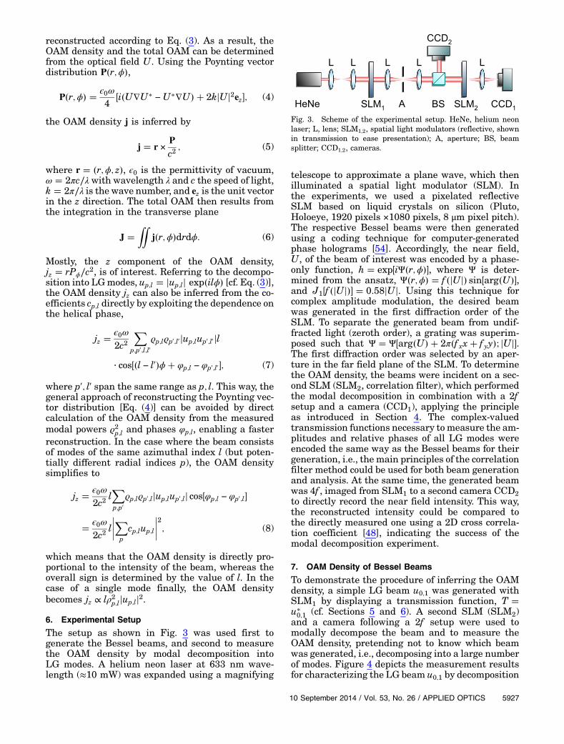
The setup as shown in Fig. 3 was used first togenerate the Bessel beams, and second to measurethe OAM density by modal decomposition intoLG modes. A helium neon laser at 633 nm wave-length (≈10 mW) was expanded using a magnifying

telescope to approximate a plane wave, which thenilluminated a spatial light modulator (SLM). Inthe experiments, we used a pixelated reflectiveSLM based on liquid crystals on silicon (Pluto,Holoeye, 1920 pixels ×1080 pixels, 8 μm pixel pitch).The respective Bessel beams were then generatedusing a coding technique for computer-generatedphase holograms [54]. Accordingly, the near field,U, of the beam of interest was encoded by a phase-only function, h � exp�iΨ�r;ϕ��, where Ψ is deter-mined from the ansatz, Ψ�r;ϕ� � f �jUj� sin�arg�U��,and J1�f �jUj�� 0.58jUj. Using this technique forcomplex amplitude modulation, the desired beamwas generated in the first diffraction order of theSLM. To separate the generated beam from undif-fracted light (zeroth order), a grating was superim-posed such that Ψ � Ψ�arg�U� � 2π�f xx� f yy�; jUj�.The first diffraction order was selected by an aper-ture in the far field plane of the SLM. To determinethe OAM density, the beams were incident on a sec-ond SLM (SLM2, correlation filter), which performedthe modal decomposition in combination with a 2fsetup and a camera (CCD1), applying the principleas introduced in Section 4. The complex-valuedtransmission functions necessary tomeasure the am-plitudes and relative phases of all LG modes wereencoded the same way as the Bessel beams for theirgeneration, i.e., the main principles of the correlationfilter method could be used for both beam generationand analysis. At the same time, the generated beamwas 4f , imaged from SLM1 to a second camera CCD2to directly record the near field intensity. This way,the reconstructed intensity could be compared tothe directly measured one using a 2D cross correla-tion coefficient [48], indicating the success of themodal decomposition experiment.

7. OAM Density of Bessel Beams

To demonstrate the procedure of inferring the OAMdensity, a simple LG beam u0;1 was generated withSLM1 by displaying a transmission function, T �u�0;1 (cf. Sections 5 and 6). A second SLM (SLM2)

and a camera following a 2f setup were used tomodally decompose the beam and to measure theOAM density, pretending not to know which beamwas generated, i.e., decomposing into a large numberof modes. Figure 4 depicts the measurement resultsfor characterizing the LG beam u0;1 by decomposition

Fig. 3. Scheme of the experimental setup. HeNe, helium neonlaser; L, lens; SLM1;2, spatial light modulators (reflective, shownin transmission to ease presentation); A, aperture; BS, beamsplitter; CCD1;2, cameras.


into LG modes of the same intrinsic scale,w � 0.3 mm, and of indices l � −3…3 andp � 0…10. In Fig. 4(a) the modal spectrum revealsthe content of one single mode, which is the u0;1mode, as expected. In addition to the power spectrumthe relative phases of all modes were measured andthe beam intensity was reconstructed using Eq. (3).Figure 4(b) shows the typical ring-shaped intensity,which is in good agreement with the directly mea-sured beam intensity (CCD2, inset). The measuredOAM density in units of Nsm−2 is depicted inFig. 4(c) in addition to the theoretical OAM density,revealing good agreement. The fact that the OAMdensity and beam intensity look identical can beunderstood from Eq. (8), which elucidates that theOAM density is directly proportional to the intensityfor beams of a single l value. For the same reason, theOAM density is all positive and does not change signwithin the whole measurement area, caused by thepositive sign of l [Eq. (8)]. By choosing the same in-trinsic scale of the generated beam and decomposi-tion modes, the mode set is perfectly adapted,yielding a single response in the mode spectrum.This is completely different when a Bessel beam ofthe same azimuthal index, l � 1 (intrinsic radiuswb � 0.2 mm), is decomposed into LG modes(w � 0.3 mm), which is shown in Fig. 5. As outlinedin Section 3, when decomposing a Bessel beam intoLG modes, only those modes of equal azimuthal in-dex appear, which is confirmed by the modal powerspectrum in Fig. 5(a). In contrast to the previous

example in Fig. 4, however, those modes are dis-persed over a range of radial indices, p. The numberof relevant modes found in the experiment is in goodagreement with the prediction of Fig. 1. Note that thechosen range of p values (p � 0…10) is slightly largerthan the actual required number of modes given inFig. 1, at w � 0.3 mm. This was done to prove thatthe chosen range of mode indices is sufficient forreconstruction, i.e., some of the modes can be ne-glected. Again, from modal amplitudes and phases,the beam intensity [Fig. 5(b)] and OAM density[Fig. 5(c)] were reconstructed, matching the directlymeasured intensity and the theoretical OAM density.As in the previous case, the intensity distribution re-sembles the OAM density, and the OAM density isentirely positive, although the beam consists of asum of modes. This is because only one azimuthalindex, l, is involved in the superposition, wherethe OAM density is directly proportional to the beamintensity and l, according to Eq. (8).

To demonstrate that the decomposition of Besselbeams in LG modes is a versatile approach, we gen-erated two different superpositions of Bessel beamsyielding more complicated OAM density distribu-tions. First, we considered an equally weightedsuperposition of two Bessel beams of opposite handi-ness in phase J3�q1r� exp�3iϕ� � J

−3�q2r� exp�−3iϕ�(wb � 0.2 mm), and decomposed it into LG modes,with w � 0.5 mm as depicted in Fig. 6. In the modespectrum now two traces of radial modes can beseen at l � 3 and l � −3. The corresponding intensity

Fig. 4. Modal decomposition of an LG beam, u0;1. (a) Modespectrum. Reconstruction of (b) beam intensity and (c) OAMdensity. The insets depict the measured beam intensity and theo-retical OAM density, respectively. The depicted section is2.4 mm× 2.4 mm.

Fig. 5. Modal decomposition of a Bessel beam, J1 exp�iϕ�.(a) Mode spectrum. Reconstruction of (b) beam intensity and (c)OAM density. The insets depict the measured beam intensityand theoretical OAM density, respectively. The depicted sectionis 2.4 mm× 2.4 mm.


pattern consists of six petals that are formed by thecoherent Bessel superposition [cf. Fig. 6(b)]. If thescale of both Bessel beams were chosen to be exactlythe same, the OAM density would vanish at everypoint of the field. For this reason, we detuned thescale of both beams slightly to yield an OAM densitythat oscillates between positive and negative parts,as shown in Fig. 6(c). As a result, the OAM densityand beam intensity differ from each other, since morethan one azimuthal index l is involved in the super-position. Although the correlation of the measuredand theoretical OAM density is very good, it is notice-able that the OAM reconstruction becomes fainttoward the rim. This is a direct result of both thelimited extension of the LG modes compared to theBessel beam and the restriction to a finite numberof modes. Reconstruction within a larger regionwould, consequently, require the use of more modesfor decomposition.

A superposition of four Bessel beams,J2�q1r�exp�2iϕ��J1�q2r�exp�iϕ��J

−1�q3r�exp�−iϕ��J−2�q4r�exp�−2iϕ� is shown in Fig. 7. Again, each

single Bessel beam was slightly detuned in scale,aroundwb � 0.2 mm, and characterized by decompo-sition into LG modes of intrinsic scale, w � 0.5 mm.This time, four traces of radial modes appear in thespectrum [Fig. 7(a)]. As a result of the superpositionthe intensity becomes asymmetric [Fig. 7(b)],whereas the OAM density distribution is split into

two halves with oscillations with opposed signs[Fig. 7(c)]. Again, beam intensity and OAM densityare dissimilar due to the inclusion of several azimu-thal modes of different l. Both beam intensity andOAM density are in very good agreement with thedirectly measured intensity and the theoreticalOAM density distribution, revealing the high accu-racy achieved with the modal decomposition.

8. Comparison to Azimuthal Decomposition

Besides the correlation-based modal decomposi-tion, the only other technique for OAM densityreconstruction is the azimuthal decomposition [16].It is hence worthwhile to compare the achievedresults to the example of Bessel beams.

The azimuthal decomposition technique is basedon the same principle as the modal decompositiontechnique by means of an all-optical inner productmeasurement performed by correlation or matchedfilters (cf. Section 4). The only difference betweenthe two types of decomposition lies in the definitionof the matched filter. Unlike the modal decomposi-tion, which requires the matched filter to be assignedas a 2D orthonormal basis (e.g., LG basis functions),the matched filter for the azimuthal decomposition isdescribed in terms of 1D azimuthal phase variations,exp�ilϕ�. In analogy to Eq. (3), the optical field,U, canhence be described as [43]

Fig. 6. Modal decomposition of a symmetric superposition ofBessel beams, J3�q1r� exp�3iϕ� � J

−3�q2r� exp�−3iϕ�. (a) Modespectrum. Reconstruction of (b) beam intensity and (c) OAMdensity. The insets depict the measured beam intensity andtheoretical OAM density, respectively. The depicted section is2.4 mm× 2.4 mm.

Fig. 7. Modal decomposition of a nonsymmetric super-position of Bessel beams, J2�q1r� exp�2iϕ� � J1�q2r� exp�iϕ��J−1�q3r� exp�−iϕ� � J

−2�q4r� exp�−2iϕ�. (a) Mode spectrum.Reconstruction of (b) beam intensity and (c) OAM density. Theinsets depict the measured beam intensity and theoretical OAMdensity, respectively. The depicted section is 2.4 mm× 2.4 mm.


U�r;ϕ� �Xl

cl�r� exp�ilϕ�; (9)

where cl�r� � ϱl�r� exp�iφl�r��. Note that a radialindex is not necessary here. Instead, the radialdependence is moved into the expansion coefficientcl�r�, which is in contrast to Eq. (3), where cp;l is aconstant for given indices, p and l. The outstandingbenefit of this azimuthal decomposition is the inde-pendence of the basis functions exp�ilϕ� from the spa-tial scale, which was discussed in Section 3 as thecrucial parameter when using a correlation filter,since it influences the signal-to-noise ratio and thenumber of modes and hence the required measure-ment time [49]. The advantage of this scale invari-ance is accompanied by the need for restoring theradial dependence of the beam by other means.Accordingly, the azimuthal matched filter functionexp�ilϕ� must be bounded by a ring-slit,

Tl�r;ϕ� ��exp�ilϕ� R −

ΔR2 < r < R� ΔR

20 otherwise

; (10)

whose width ΔR represents the spatial resolutionwith which the OAM density can finally be recon-structed [43]. With these azimuthal matched filters,the amplitude functions ρl�r� associated with eachazimuthal mode exp�ilϕ� at a set radial coordinater can be extracted [55]. Similarly, their relative phasefunctions φl�r� are inferred from the interference ofthe azimuthal mode exp�ilϕ� with a reference wave,which may be implemented as an external sourceor, for convenience, the first mode in the series,l � 0, at a specific value of r [43]. The quantitativeOAM density of a field is then determined in com-plete analogy to the derivations in Section 5 by eitherreconstructing the field or by calculating it directlyfrom the azimuthal decomposition [16], similar toEq. (7).

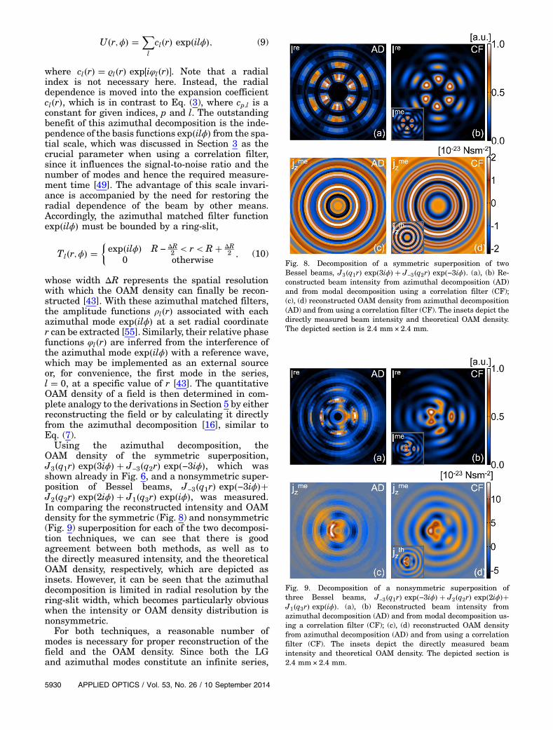
Using the azimuthal decomposition, theOAM density of the symmetric superposition,J3�q1r� exp�3iϕ� � J

−3�q2r� exp�−3iϕ�, which wasshown already in Fig. 6, and a nonsymmetric super-position of Bessel beams, J

−3�q1r� exp�−3iϕ��J2�q2r� exp�2iϕ� � J1�q3r� exp�iϕ�, was measured.In comparing the reconstructed intensity and OAMdensity for the symmetric (Fig. 8) and nonsymmetric(Fig. 9) superposition for each of the two decomposi-tion techniques, we can see that there is goodagreement between both methods, as well as tothe directly measured intensity, and the theoreticalOAM density, respectively, which are depicted asinsets. However, it can be seen that the azimuthaldecomposition is limited in radial resolution by thering-slit width, which becomes particularly obviouswhen the intensity or OAM density distribution isnonsymmetric.

For both techniques, a reasonable number ofmodes is necessary for proper reconstruction of thefield and the OAM density. Since both the LGand azimuthal modes constitute an infinite series,

Fig. 8. Decomposition of a symmetric superposition of twoBessel beams, J3�q1r� exp�3iϕ� � J

−3�q2r� exp�−3iϕ�. (a), (b) Re-constructed beam intensity from azimuthal decomposition (AD)and from modal decomposition using a correlation filter (CF);(c), (d) reconstructed OAM density from azimuthal decomposition(AD) and from using a correlation filter (CF). The insets depict thedirectly measured beam intensity and theoretical OAM density.The depicted section is 2.4 mm× 2.4 mm.

Fig. 9. Decomposition of a nonsymmetric superposition ofthree Bessel beams, J

−3�q1r� exp�−3iϕ� � J2�q2r� exp�2iϕ��J1�q3r� exp�iϕ�. (a), (b) Reconstructed beam intensity fromazimuthal decomposition (AD) and from modal decomposition us-ing a correlation filter (CF); (c), (d) reconstructed OAM densityfrom azimuthal decomposition (AD) and from using a correlationfilter (CF). The insets depict the directly measured beamintensity and theoretical OAM density. The depicted section is2.4 mm× 2.4 mm.


selecting these modes when executing either decom-position might pose a challenge if one has no priorknowledge of the field. In this case, both techniquescan be approached in an iterative (although time-consuming) manner as outlined in Section 3. An es-timation of the azimuthal modes present in the fieldcan again be obtained by displaying the respectivephase patterns, exp�ilϕ�, (without amplitude modu-lation) and scanning through different values of l.As implied by Eq. (9), for the azimuthal decomposi-tion technique, a range of radial coordinates, r, willneed to be sampled when reconstructing a field (be iteither Bessel or LG), but the choice of the ring-slitwidth and the number of ring-slits sampled will dic-tate the resolution and quality of the reconstructedfield. In comparison, the modal decomposition (whenimplementing the LG basis as the matched filter)will require the same range of azimuthal indices, l,but also require a range of radial indices, p, e.g., inorder to reconstruct the concentric ring structurepresent in Bessel beams. So, depending on the num-ber of radial indices required for modal decomposi-tion, either one of the techniques can be faster. Inthe presented examples, however, the beams weresampled with about 30 ring-slits regarding the azi-muthal decomposition, whereas 10 radial LG modeswere used with the correlation filter. For each radialmode, and for each ring-slit, respectively, the phasedelay was measured in addition to the amplitude.Accordingly, the number of correlation measure-ments for the investigated beams was reduced bya factor of three when using the correlation filter-based modal decomposition, yielding a measurementduration of about 1 min. For both techniques, themeasurement process could be sped up by angularmultiplexing the single transmission functions, asdetailed in [53]. However, for simplicity, all phasepatterns were displayed, subsequently, on the corre-sponding SLM (SLM2, cf. Section 6 and Fig. 3).

In terms of spatial resolution, the resolution ofthe SLM of 8 μm is finally limiting for both tech-niques (cf. Section 6). In the case of the correlationfilter, the OAM density was hence reconstructed with300 pixels × 300 pixels, whereas, for the azimuthaldecomposition, the number of sampled ring-slits isthe critical parameter. In the experiments the radialresolution was set to about 80 μm. In principle, theradial resolution could be improved by correlatingthe incident field with thinner ring-slits. However,this will simultaneously yield a significant drop intransmitted power and hence complicate detection.In comparison, the transmitting area is much largerwhen displaying an LGmode, such that the signal-to-noise ratio is, generally, larger using the correlationfilter.

Even though the modal decomposition is advanta-geous in terms of spatial resolution and signal-to-noise ratio, this technique is scale-dependent: ifthe scale parameter,w, of the LGmodes is incorrectlyselected, this will translate into an unnecessary largenumber of modes and hence into a worse signal-

to-noise ratio and longer measurement durations,rendering its benefits void. To circumvent this limi-tation, in addition to choosing a suitable mode basis,its spatial scale should be determined by measuringthe beam propagation ratio and beam diameter,which can be done digitally using the same setupas shown in Fig. 3 [49] (cf. Section 3). The azimuthaldecomposition on the other side overcomes this issueof scale dependence, but at the cost of spatial resolu-tion, signal-to-noise ratio, and computation time;more ring-slits (i.e., matched filters) are required forsensible reconstruction.

9. Conclusion

To summarize, we demonstrated the quantitativeOAM density measurement on pure and superim-posed Bessel beams by projection into Laguerre–Gaussian (LG) modes. The projection was realizedby modal decomposition with correlation filters. Incontrast to previous studies, it was shown that suchdecomposition is not limited to superpositions of LGbeams but can equally be used to characterize arbi-trary beam shapes, such as superpositions of Besselbeams. By choosing the spatial scale of the LG basiscorrectly, the number of radial modes necessary to re-construct the OAM density can be small; e.g., aboutten radial modes were required in the presented ex-periments. In comparison to the previously publishedazimuthal decomposition, the decomposition into LGmodes stands out by its high spatial resolution,reduced measurement time, and improved signal-to-noise ratio. In contrast, the main benefit of theazimuthal decomposition is its independence of thespatial scale, which must be determined separatelyby an additional measurement concerning the modaldecomposition technique. Given the spatial scale, thecorrelation filter-based modal decomposition enablesa fast and robust measurement of the OAM densityeven in the case of highly multimode fields, whereasreconstruction fidelities of up to 95% were reached.

References1. L. Allen, M. W. Beijersbergen, R. J. C. Spreeuw, and J. P.

Woerdman, “Orbital angular momentum of light and thetransformation of Laguerre-Gaussian laser modes,” Phys.Rev. A 45, 8185–8189 (1992).

2. M. Padgett, J. Courtial, and L. Allen, “Light’s orbital angularmomentum,” Phys. Today 57(5), 35–40 (2004).

3. S. Franke-Arnold, L. Allen, and M. Padgett, “Advances in op-tical angular momentum,” Laser Photon. Rev. 2, 299–313(2008).

4. A. M. Yao and M. J. Padgett, “Orbital angular momentum: ori-gins, behavior and applications,” Adv. Opt. Photon. 3, 161–204(2011).

5. M. E. J. Friese, J. Enger, H. Rubinsztein-Dunlop, and N. R.Heckenberg, “Optical angular-momentum transfer to trappedabsorbing particles,” Phys. Rev. A 54, 1593–1596 (1996).

6. V. Garcés-Chávez, D. McGloin, M. J. Padgett, W. Dultz, H.Schmitzer, and K. Dholakia, “Observation of the transfer ofthe local angular momentum density of a multiringed lightbeam to an optically trapped particle,” Phys. Rev. Lett. 91,093602 (2003).

7. Y. Zhao, D. Shapiro, D. Mcgloin, D. T. Chiu, and S. Marchesini,“Direct observation of the transfer of orbital angular momen-tum to metal particles from a focused circularly polarizedGaussian beam,” Opt. Express 17, 23316–23322 (2009).


8. K. Dholakia and T. Cizmar, “Shaping the future of manipula-tion,” Nat. Photonics 5, 335–342 (2011).

9. M. Padgett and R. Bowman, “Tweezers with a twist,” Nat.Photonics 5, 343–348 (2011).

10. R. Fickler, R. Lapkiewicz, W. N. Plick, M. Krenn, C. Schaeff, S.Ramelow, and A. Zeilinger, “Quantum entanglement of highangular momenta,” Science 338, 640–643 (2012).

11. G. Gibson, J. Courtial, M. Padgett, M. Vasnetsov, V. Pas’ko, S.Barnett, and S. Franke-Arnold, “Free-space informationtransfer using light beams carrying orbital angular momen-tum,” Opt. Express 12, 5448–5456 (2004).

12. J. Wang, J.-Y. Yang, I. M. Fazal, N. Ahmed, Y. Yan, H. Huang,Y. Ren, Y. Yue, S. Dolinar, M. Tur, and A. E. Willner,“Terabit free-space data transmission employing orbital angu-lar momentum multiplexing,” Nat. Photonics 6, 488–496(2012).

13. N. Bozinovic, Y. Yue, Y. Ren, M. Tur, P. Kristensen, H. Huang,A. E. Willner, and S. Ramachandran, “Terabit-scale orbitalangular momentum mode division multiplexing in fibers,”Science 340, 1545–1548 (2013).

14. L. Allen and M. J. Padgett, “The Poynting vector in Laguerre-Gaussian beams and the interpretation of their angularmomentum density,” Opt. Commun. 184, 67–71 (2000).

15. N. Bozinovic, S. Golowich, P. Kristensen, and S.Ramachandran, “Control of orbital angular momentumof light with optical fibers,” Opt. Lett. 37, 2451–2453(2012).

16. A. Dudley, I. A. Litvin, and A. Forbes, “Quantitative measure-ment of the orbital angular momentum density of light,” Appl.Opt. 51, 823–833 (2012).

17. I. A. Litvin, M. G. McLaren, and A. Forbes, “A conical waveapproach to calculating Bessel-Gauss beam reconstructionafter complex obstacles,” Opt. Commun. 282, 1078–1082(2009).

18. M. McLaren, T. Mhlanga, M. J. Padgett, F. S. Roux, and A.Forbes, “Self-healing of quantum entanglement after an ob-struction,” Nat. Commun. 5, 1–8 (2014).

19. K. Volke-Sepulveda, V. Garcés-Chávez, S. Chávez-Cerda, J.Arlt, and K. Dholakia, “Orbital angular momentum of ahigh-order Bessel light beam,” J. Opt. B 4, S82–S89 (2002).

20. W.M. Lee, X.-C. Yuan, andW. C. Cheong, “Optical vortex beamshaping by use of highly efficient irregular spiral phase platesfor optical micromanipulation,” Opt. Lett. 29, 1796–1798(2004).

21. M. Mirhosseini, O. S. Magaña-Loaiza, C. Chen, B. Rodenburg,M. Malik, and R. W. Boyd, “Rapid generation of light beamscarrying orbital angular momentum,” Opt. Express 21,30196–30203 (2013).

22. M. Zurch, C. Kern, P. Hansinger, A. Dreischuh, and C.Spielmann, “Strong-field physics with singular light beams,”Nat. Phys. 8, 743–746 (2012).

23. B. J. McMorran, A. Agrawal, I. M. Anderson, A. A. Herzing,H. J. Lezec, J. J. McClelland, and J. Unguris, “Electron vortexbeams with high quanta of orbital angular momentum,”Science 331, 192–195 (2011).

24. J. Courtial, K. Dholakia, L. Allen, and M. Padgett, “Gaussianbeams with very high orbital angular momentum,” Opt.Commun. 144, 210–213 (1997).

25. S.-C. Chu, T. Ohtomo, and K. Otsuka, “Generation of dough-nutlike vortex beam with tunable orbital angular momentumfrom lasers with controlled Hermite-Gaussian modes,” Appl.Opt. 47, 2583–2591 (2008).

26. T. Yusufu, Y. Tokizane, M. Yamada, K. Miyamoto, and T.Omatsu, “Tunable 2-μm optical vortex parametric oscillator,”Opt. Express 20, 23666–23675 (2012).

27. M. Koyama, T. Hirose, M. Okida, K.Miyamoto, and T. Omatsu,“Power scaling of a picosecond vortex laser based on a stressedYb-doped fiber amplifier,” Opt. Express 19, 994–999(2011).

28. A. Mair, A. Vaziri, G. Weihs, and A. Zeilinger, “Entanglementof the orbital angular momentum states of photons,” Nature412, 313–316 (2001).

29. C. Smith and R. McDuff, “Charge and position detection ofphase singularities using holograms,” Opt. Commun. 114,37–44 (1995).

30. P. Genevet, J. Lin, M. A. Kats, and F. Capasso, “Holographicdetection of the orbital angular momentum of lightwith plasmonic photodiodes,” Nat. Commun. 3, 1278(2012).

31. J. M. Hickmann, E. J. S. Fonseca, W. C. Soares, and S.Chávez-Cerda, “Unveiling a truncated optical lattice associ-ated with a triangular aperture using light’s orbital angularmomentum,” Phys. Rev. Lett. 105, 053904 (2010).

32. J. Courtial, K. Dholakia, D. A. Robertson, L. Allen, and M. J.Padgett, “Measurement of the rotational frequency shiftimparted to a rotating light beam possessing orbital angularmomentum,” Phys. Rev. Lett. 80, 3217–3219 (1998).

33. M. V. Vasnetsov, J. P. Torres, D. V. Petrov, and L. Torner,“Observation of the orbital angular momentum spectrum ofa light beam,” Opt. Lett. 28, 2285–2287 (2003).

34. J. Leach, M. J. Padgett, S. M. Barnett, S. Franke-Arnold, andJ. Courtial, “Measuring the orbital angular momentum of asingle photon,” Phys. Rev. Lett. 88, 257901 (2002).

35. M. P. J. Lavery, A. Dudley, A. Forbes, J. Courtial, and M. J.Padgett, “Robust interferometer for the routing of light beamscarrying orbital angular momentum,” New J. Phys. 13,093014 (2011).

36. A. Belmonte and J. P. Torres, “Digital coherent receiver fororbital angular momentum demultiplexing,” Opt. Lett. 38,241–243 (2013).

37. V. P. Aksenov, I. V. Izmailov, F. Y. Kanev, and B. N. Poizner,“Optical vortex detector as a basis for a data transfer system:operational principle, model, and simulation of the influenceof turbulence and noise,” Opt. Commun. 285, 905–928(2012).

38. G. C. G. Berkhout, M. P. J. Lavery, J. Courtial, M. W.Beijersbergen, and M. J. Padgett, “Efficient sorting of orbitalangular momentum states of light,” Phys. Rev. Lett. 105,153601 (2010).

39. M. P. J. Lavery, G. C. G. Berkhout, J. Courtial, and M. J.Padgett, “Measurement of the light orbital angular momen-tum spectrum using an optical geometric transformation,”J. Opt. 13, 064006 (2011).

40. M. P. J. Lavery, D. J. Robertson, A. Sponselli, J. Courtial, N. K.Steinhoff, G. A. Tyler, A. Wilner, and M. J. Padgett, “Efficientmeasurement of an optical orbital-angular-momentum spec-trum comprising more than 50 states,” New J. Phys. 15,013024 (2013).

41. A. Dudley, T. Mhlanga, M. Lavery, A. McDonald, F. S. Roux, M.Padgett, and A. Forbes, “Efficient sorting of Bessel beams,”Opt. Express 21, 165–171 (2013).

42. M. P. J. Lavery, D. J. Robertson, G. C. G. Berkhout, G. D. Love,M. J. Padgett, and J. Courtial, “Refractive elements for themeasurement of the orbital angular momentum of a singlephoton,” Opt. Express 20, 2110–2115 (2012).

43. I. A. Litvin, A. Dudley, F. S. Roux, and A. Forbes, “Azimuthaldecomposition with digital holograms,” Opt. Express 20,10996–11004 (2012).

44. C. Schulze, A. Dudley, D. Flamm, M. Duparré, and A. Forbes,“Measurement of the orbital angular momentum density oflight by modal decomposition,” New J. Phys. 15, 073025(2013).

45. J. C. Gutiérrez-Vega, M. D. Iturbe-Castillo, and S. Chávez-Cerda, “Alternative formulation for invariant optical fields:Mathieu beams,” Opt. Lett. 25, 1493–1495 (2000).

46. M. A. Bandres and J. Gutiérrez-Vega, “Ince-Gaussian beams,”Opt. Lett. 29, 144–146 (2004).

47. J. W. Goodman, Introduction to Fourier Optics, 3rd ed.(Roberts & Company, 2005).

48. J. L. Rodgers and W. A. Nicewander, “Thirteen ways to look atthe correlation coefficient,” Am. Stat. 42, 59–66 (1988).

49. C. Schulze, S. Ngcobo, M. Duparré, and A. Forbes, “Modal de-composition without a priori scale information,” Opt. Express20, 27866–27873 (2012).

50. A. E. Siegman, “New developments in laser resonators,” Proc.SPIE 1224, 2–14 (1990).

51. M. A. Golub, A. M. Prokhorov, I. N. Sisakian, and V. A. Soifer,“Synthesis of spatial filters for investigation of the transversemode composition of coherent radiation,” Sov. J. QuantumElectron. 9, 1866–1868 (1982).


52. H. Bartelt, A. Lohmann, W. Freude, and G. Grau, “Modeanalysis of optical fibres using computer-generated matchedfilters,” Electron. Lett. 19, 247–249 (1983).

53. T. Kaiser, D. Flamm, S. Schröter, and M. Duparré, “Completemodal decomposition for optical fibers using CGH-based cor-relation filters,” Opt. Express 17, 9347–9356 (2009).

54. V. Arrizón, U. Ruiz, R. Carrada, and L. A. González, “Pixelatedphase computer holograms for the accurate encoding of scalarcomplex fields,” J. Opt. Soc. Am. A 24, 3500–3507 (2007).

55. I. A. Litvin, A. Dudley, and A. Forbes, “Poynting vector andorbital angular momentum density of superpositions of Besselbeams,” Opt. Express 19, 16760–16771 (2011).


measurement of the orbital angular momentum density of...

Documents