measurement of phased array point spread functions for … · 1 american institute of aeronautics...

1

American Institute of Aeronautics and Astronautics

Measurement of Phased Array Point Spread Functions

for use with Beamforming

Chris Bahr,* Nikolas S. Zawodny,

† Brandon Bertolucci,

† Kyle Woolwine,

‡

Fei Liu,§ Jian Li,

** Mark Sheplak,

†† and Louis Cattafesta

††

Florida Center for Advanced Aero-Propulsion

Interdisciplinary Microsystems Group

University of Florida, Gainesville, FL 32611

Microphone arrays can be used to localize and estimate the strengths of acoustic sources

present in a region of interest. However, the array measurement of a region, or beam map,

is not an accurate representation of the acoustic field in that region. The true acoustic field

is convolved with the array’s sampling response, or point spread function (PSF). Many

techniques exist to remove the PSF’s effect on the beam map via deconvolution. Currently

these methods use a theoretical estimate of the array point spread function and perhaps

account for installation offsets via determination of the microphone locations. This

methodology fails to account for any reflections or scattering in the measurement setup and

still requires both microphone magnitude and phase calibration, as well as a separate shear

layer correction in an open-jet facility. The research presented seeks to investigate direct

measurement of the array’s PSF using a non-intrusive acoustic point source generated by a

pulsed laser system. Experimental PSFs of the array are computed for different conditions

to evaluate features such as shift-invariance, shear layers and model presence. Results show

that experimental measurements trend with theory with regard to source offset. The source

shows expected behavior due to shear layer refraction when observed in a flow, and

application of a measured PSF to NACA 0012 aeroacoustic trailing-edge noise data shows a

promising alternative to a classic shear layer correction method.

I. Introduction

N aeroacoustic wind tunnel testing, phased microphone arrays have become common instrumentation. Phased

array techniques apply a source model to data measured from a sensor array and generate a map of estimates of

source locations and strengths [1]. Unfortunately, the conventional beamformer output using the delay-and-sum

technique, or any variant thereof, is convolved with the array’s point spread function [2]. This point spread function

(PSF) arises due to the array’s finite aperture and finite sample locations, and is a representation of the array’s

output response to an ideal point source at a given location in space. The PSF is a function of frequency and, except

for the special case of a plane wave field, is not shift-invariant to the source location.

* Research Aerospace Engineer, Aeroacoustics Branch, NASA Langley Research Center, Hampton, VA

23681, Member AIAA (Formerly Post-Doctoral Research Associate at University of Florida, where

research was conducted) † Graduate Research Assistant, MAE Department, P.O. Box 116250, Student Member AIAA

‡ Undergraduate Research Assistant, MAE Department, P.O. Box 116250, Student Member AIAA

§ Research Scientist, MAE Department, P.O. Box 116250, Member AIAA

** Professor, ECE Department, P.O. Box 116200

†† Professor, MAE Department, P.O. Box 116250, Associate Fellow AIAA, [email protected]

I

https://ntrs.nasa.gov/search.jsp?R=20110012475 2018-05-28T06:52:46+00:00Z

2


Multiple methods exist to attempt to remove the effects of the PSF from a beamformer output, or beam map. A

non-exhaustive list of the current methods in use includes DAMAS [3], DAMAS2 [4], FFT-NNLS [5], CLEAN-SC

[6], CMF [7], LORE [8] and MACS [9]. DAMAS, CMF, LORE and MACS formulate the deconvolution problem

as the solution to a large system of equations. These methods allow for a variable PSF through varying steering

vector terms but may be computationally intensive depending on the problem of interest. DAMAS2 and FFT-NNLS

treat the deconvolution problem as an image processing technique and attempt to iteratively divide out the effects of

the PSF in a Fourier transform of the original beam map and PSF, similar to the Weiner Filter [4]. The original

formulation of these requires a shift-invariant PSF, but the algorithms can be modified to allow variation [5, 10].

Shift-invariance assumes that the PSF’s shape does not change with source location, and that the overall beam

pattern is simply shifted in space [4]. CLEAN-SC is the only method from those listed above which does not use an

explicit deconvolution approach, instead modifying the beam map to remove coherent sidelobe contributions.

For all of the mentioned methods that use the PSF, an ideal theoretical PSF based on the array design is generally

used. Array calibration, both individual and group, is handled before deconvolution occurs. Individual channel

calibration, compensating for magnitude and phase offsets in each element of the array, is often done ahead of time

and applied in the construction of the cross-spectral matrix, prior to beamforming. Group calibration can

alternatively correct for microphone magnitude and phase offsets and compensate for small positional errors in

microphone placement when shift-invariance is assumed. This technique can correct the steering vectors used in

conventional beamforming [2]. Corrections for shear layers, when conducting experiments in open-jet wind tunnels,

[11] are also applied using the conventional steering vectors. None of these methods directly account for real

installation effects such as reflections and scattering, which alter the appropriate Helmholtz equation solution (as all

of these analysis techniques apply to the frequency domain free-field boundary conditions).

The PSF is generally treated as the array’s response function to a point source input, often observed in the

frequency domain [4]. It can also be considered as the array’s observation of the response function of a test setup

[13] for a particular source location, similar to a single observation of the installation’s Green’s function. In this

sense, the theoretical PSF with standard corrections applied may fall short of truly characterizing the observed array

response for a point source. Due to the computational complexity of determining the point source response of a real

experimental setup for all frequencies of interest, experiments provide the most promising route for evaluating the

true PSF.

Some previous research has been conducted regarding experimental analysis of PSFs. PSF analysis and

deconvolution have a long history in the fields of optics and radio astronomy [4]. Dougherty’s work on group

calibration can be considered an approximation of a measurement of a free-space Green’s function [2]. Dougherty

also discussed the effects of reverberant walls in a reverberant facility on phased array output. Oerlemans and

Sijtsma experimentally studied the effect of reverberant sidewalls in an open jet wind tunnel on phased array output

[12]. Fenech and Takeda measured the appropriate Green’s function for a reverberant facility to compare with an

image source correction to the free-space Green’s function [13]. In both cases, computing an in-situ experimental

correction improved beamforming performance. Both of these experiments, however, used intrusive acoustic

sources which precluded measurements from occurring when test section flow was present. The present study, in

contrast, uses a non-intrusive analysis method which can be used both with and without flow, allowing shear layer

corrections to be experimentally incorporated into approximate point spread functions [14].

This paper first presents the development of the theoretical PSF for a spherical wave beamformer. It then

describes how an experimental PSF measurement can be used with image-processing based deconvolution and in the

formulation of experimental steering vectors. The experimental setup is then described for measuring an acoustic

point source generated by a pulsed laser system under different conditions. Results are presented for varying

3


experimental conditions, including different physical facility and model configurations, as well as mean flow effects,

before being used to correct an aeroacoustic measurement. Conclusions and future work follow.

II. Theoretical Development and Implementation

In phased array analysis, a microphone array, like the one shown in Figure 1 and Figure 2, is used to sample an

acoustic field in space and time. The data from the array measurement are acquired and, for conventional

beamforming and all its derivatives, averaged to obtain auto- and cross-power estimates in the form of a cross-

spectral matrix (CSM). Consider an M-element array, with subscript m denoting a given microphone within the

array, and subscript 0 denotes the array center at Cartesian origin (0,0,0). For a given frequency, the conventional

beamforming equation for power P from scan point l using a CSM is given by [15]

2

1, 1,H

l l lP a Ga l LM

= =�

� �

… . (1)

Here,

,1 ,

,1 ,

,0

1l l M

Tjkr jkr

l l l M

l

a r e r er

= �

⋯ (2)

is the steering vector corresponding to the thl scanning point within the region of interest. The term ,l mr is the

distance from the thl scanning point to the thm microphone (or array center in the case of m = 0), k is the acoustic

wavenumber, and the M M× matrix G�

is the CSM. Note that ( ). T and ( ). H

denote the transpose and conjugate

transpose operations, respectively. This steering vector is selected such that the beamformer output, when steered to

a correct source location in a single-source spherical-wave acoustic field, corresponds to the acoustic power

measured at the center of the array due to the source [3]. The PSF of an array can be considered the normalized

output of Equation (1) when a point source is present at scan point il , and no other sources are present. This can be

expressed where, in a 2-D scan plane a distance zs from the array face, il is located at (0,0,zs).

For image-processing based deconvolution methods, an image map of the PSF along with the experimental

delay-and-sum beam maps are the necessary inputs. The PSF map is often theoretically constructed based on the

theoretical free-field response of an array, but nothing prevents it from being an experimental measurement.

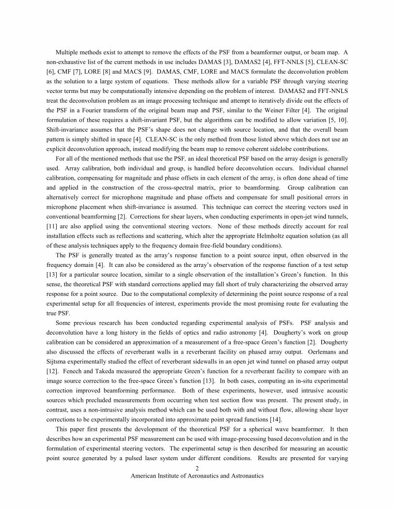
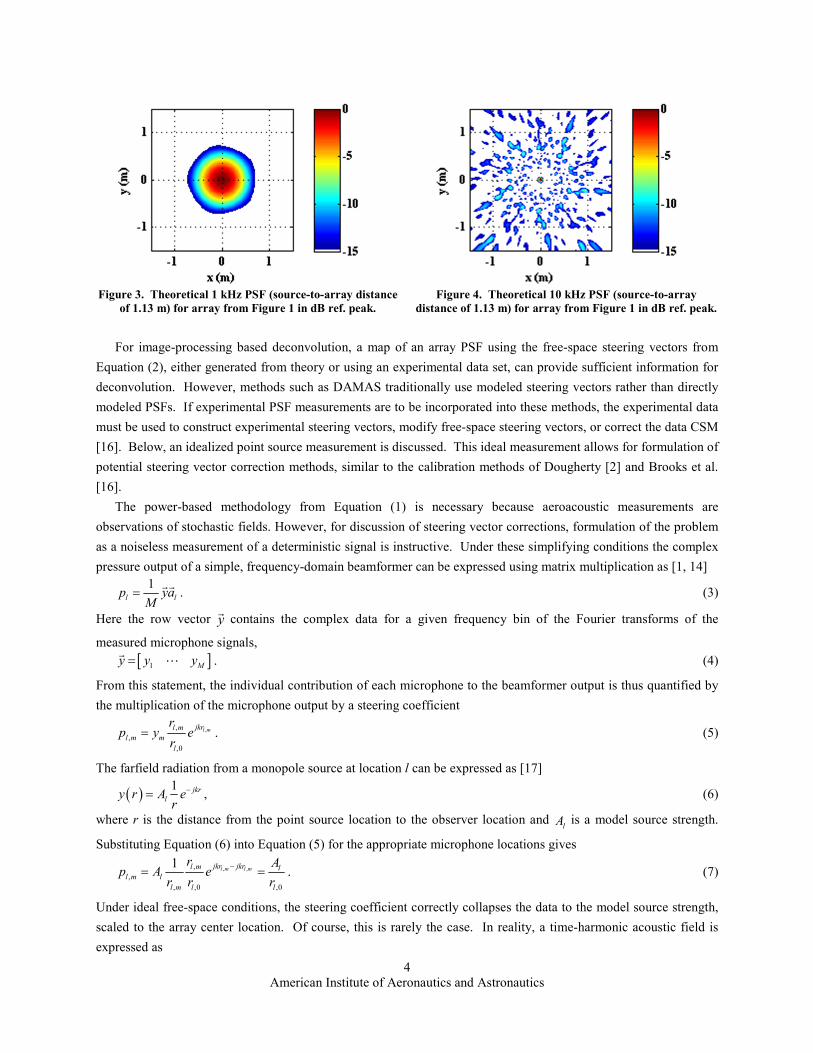
Example theoretical PSFs for the array shown in Figure 1 and Figure 2 are shown in Figure 3 and Figure 4. Note

that the spiral in Figure 2 is discontinuous on the inner ring due to a design modification, and the array is designed

for minimal sidelobes 10 dB down, but plotted on a 15 dB scale to accentuate response behavior.

Figure 1. Example free-field microphone array, prior to

application of acoustic treatment.

Figure 2. Microphone coordinates for array from Figure 1.

4


Figure 3. Theoretical 1 kHz PSF (source-to-array distance

of 1.13 m) for array from Figure 1 in dB ref. peak.

Figure 4. Theoretical 10 kHz PSF (source-to-array

distance of 1.13 m) for array from Figure 1 in dB ref. peak.

For image-processing based deconvolution, a map of an array PSF using the free-space steering vectors from

Equation (2), either generated from theory or using an experimental data set, can provide sufficient information for

deconvolution. However, methods such as DAMAS traditionally use modeled steering vectors rather than directly

modeled PSFs. If experimental PSF measurements are to be incorporated into these methods, the experimental data

must be used to construct experimental steering vectors, modify free-space steering vectors, or correct the data CSM

[16]. Below, an idealized point source measurement is discussed. This ideal measurement allows for formulation of

potential steering vector correction methods, similar to the calibration methods of Dougherty [2] and Brooks et al.

[16].

The power-based methodology from Equation (1) is necessary because aeroacoustic measurements are

observations of stochastic fields. However, for discussion of steering vector corrections, formulation of the problem

as a noiseless measurement of a deterministic signal is instructive. Under these simplifying conditions the complex

pressure output of a simple, frequency-domain beamformer can be expressed using matrix multiplication as [1, 14]

1l lp ya

M=

��

. (3)

Here the row vector y�

contains the complex data for a given frequency bin of the Fourier transforms of the

measured microphone signals,

[ ]1 My y y=�

⋯ . (4)

From this statement, the individual contribution of each microphone to the beamformer output is thus quantified by

the multiplication of the microphone output by a steering coefficient

,,

,

,0

l mjkrl m

l m m

l

rp y e

r= . (5)

The farfield radiation from a monopole source at location l can be expressed as [17]

( ) 1 jkr

ly r A er

−= , (6)

where r is the distance from the point source location to the observer location and lA is a model source strength.

Substituting Equation (6) into Equation (5) for the appropriate microphone locations gives

, ,,

,

, ,0 ,0

1l m l mjkr jkrl m l

l m l

l m l l

r Ap A e

r r r

−= = . (7)

Under ideal free-space conditions, the steering coefficient correctly collapses the data to the model source strength,

scaled to the array center location. Of course, this is rarely the case. In reality, a time-harmonic acoustic field is

expressed as

5


( ) ( ) ( )j r

ly r B r eθ=�

� �

, (8)

where source spherical symmetry is no longer enforced, and acoustic scattering and reflection can occur. Here,

( )rθ�

represents the general phase angle of the acoustic field at every point in space. Similarly,

,mj

m l my B eθ= (9)

is a general expression of the output of the mth

microphone, which can now include deviations in the microphone

position from its ideal location, as well as magnitude and phase shifts in the signal due to the microphone’s real

frequency response. Applying the ideal free-space steering coefficient to Equation (9) provides no guarantee of

properly scaling the data.

For a known source, the steering vector could be correctly computed in an experiment by measuring the

magnitude and phase shift from the source to each microphone. Unfortunately, the precise magnitude and phase of

most compact acoustic sources is immeasurable without an intrusive experimental setup. However, an alternate

approach can be employed by placing a microphone at the array center as a reference measurement. Conceptually,

the steering coefficient determines the phase angle of the acoustic field measured at a given microphone relative to

the phase angle of the field at the source location. Equation (5) can thus be re-stated as

( ),

,

,0

l mjl m

l m m

l

rp y e

r

θ θ−= . (10)

If the phase angle is subsequently shifted from the source to the array center, Equation (10) becomes

( ) ( ) ( )0 0, ,

,

,0 ,0

l m l mj j jl m l m

l m m m

l l

r rp y e e y e

r r

θ θ θ θ θ θ− − −= = . (11)

In the case of a free-space measurement where the acoustic field takes the form of Equation (6), the measurement at

an array microphone is

,

,

l mjkrl

m

l m

Ay e

r

−= (12)

while the measurement at the reference microphone is

,0

0

,0

ljkrl

l

Ay e

r

−= . (13)

Dividing Equation (13) by Equation (12) yields the frequency response between the reference microphone and the

array microphone,

( ) ( ),0 , 0, ,0

0,

,0 ,0

l l m mjk r r jl m l ml l

m

m l l l

r ry AH e e

y A r r

θ θ− − −= = = . (14)

Thus, the steering term of Equation (11) is simply the in-situ frequency response between the two microphones, and

, 0,

l

l m m mp H y= (15)

Note that in this model a constant phase angle offset, 0θ , is present in the frequency response, Equation (14). When

such steering vectors are constructed for Equation (1), this offset cancels through the multiplication of the conjugate

transpose. This frequency response function, 0,

l

mH , is a function of microphone location and performance, array

center location, source location, and installation effects for a given experimental setup. This methodology is

straightforward to implement experimentally by including a reference microphone at the array center and is

consistent with existing calibration techniques [2]. Assuming the reference microphone is calibrated to a known

standard, this steering coefficient should correct for non-idealities in the array microphone’s response, as well as

positional uncertainties, shifts due to shear layer interactions, scattering and reflections. This can be illustrated by

again using the free-space monopole model from Equation (12). Here,

6


,0

,

,

0,

,0

l

l m

jkr

l ml

m jkr

l

r eH

r e

−

−= (16)

and

,0

, ,0

,

,

, 0,

, ,0 ,0

l

l m l

l m

jkrjkr jkrl ml l l

l m m m jkr

l m l l

rA Aep y H e e

r r re

−− −

−

= = =

, (17)

recovering the expected behavior from Equation (7) with the additional expected phase offset.

Unfortunately, as mentioned above, this response function is dependent on source location, so strictly speaking

an experiment would need to be conducted with a point source sequentially traversed through every scan point in L,

and the corrected steering vector would be

, 0,1 0,

Tl l

l corr Ma H H = ⋯ . (18)

If such a measurement were conducted then this library of steering vectors could be used directly for beamforming

and potentially deconvolution. However, since large scan grids of interest make this type of measurement

intractable, this response function must instead be developed as an approximate correction to the standard free-space

steering vector. A similar correction method currently exists in the literature [2]. If shift-invariance is assumed,

which is the case when array-to-scan-plane distances are much greater than the array aperture and the scan plane

dimensions [4], the correction factor is independent of the source location (also assuming ideal, omnidirectional,

non-intrusive microphone measurements). For instance, if the response function for a centered source is defined as 2

0,

L

mH , i.e. the geometric center of the scan plane corresponds to the middle scan point index, then the corrected

steering vector could be constructed as

,1 ,

2,1 /2 ,

2 2

/ 2,0 0,1 0,

, ,1 ,

,0 2,2,1

l l M

L L M

TL L

jkr jkrL M

l corr l l Mjkr jkr

l L ML

r H Ha r e r e

r r er e

=

⋯ . (19)

When 2l L= , Equation (19) reduces to Equation (18). If this method is applied to a data set with no flow in an

anechoic enclosure, the correction factor conceptually reduces to the array calibration technique discussed by

Dougherty [2]. The method can also be used to calibrate through a shear layer on a frequency-by-frequency basis,

effectively the same way as presented by Brooks et al. [16]. As mentioned by those authors, additional corrections

are required for temperature differences between calibration measurements and aeroacoustic experiments. This

correction method assumes a non-intrusive, ideal measurement from the center reference microphone. So, for

instance, directive scattering of a center free-field microphone at high frequencies would require additional field

modeling and correction. Scattering interactions between the center microphone and array microphones would

compound the problem.

To account for varying steering vectors in space, the source can be placed at several locations within the test

section. The results of these individual measurements could, for this most simple methodology, be used to

interpolate and extrapolate a response function surface across the scan plane. Such analysis is beyond the scope of

this paper, although some research has been conducted by Suzuki which may be applied in this venue [10]. In

summary, by maintaining a reference microphone at an observation point of interest (the array center), a point

source can be used to determine what the relationship is between an array microphone and the reference

microphone, and compare that relationship to the modeled free-space relationship. This can be used ideally in place

of the modeled steering vectors, or as a lower-order model [16] as a correction to the existing steering vectors or

data.

7


III. Experimental Setup

A non-intrusive, laser-based acoustic point source is used to directly measure the point spread function of an

array in the University of Florida Aeroacoustic Flow Facility (UFAFF). This type of source has been used

previously in UFAFF [14]. Since this previous work, improvements have been made to the source.

A. Acoustic Source

An acoustic point source is generated using a pulsed laser system. The selected laser is a New Wave Solo

120XT dual Nd:YAG system, capable of outputting a maximum instantaneous energy of 120 mJ/pulse at a

wavelength of 532 nm, with a nominal pulse width of 3-5 ns. The laser beam is expanded and re-focused through a

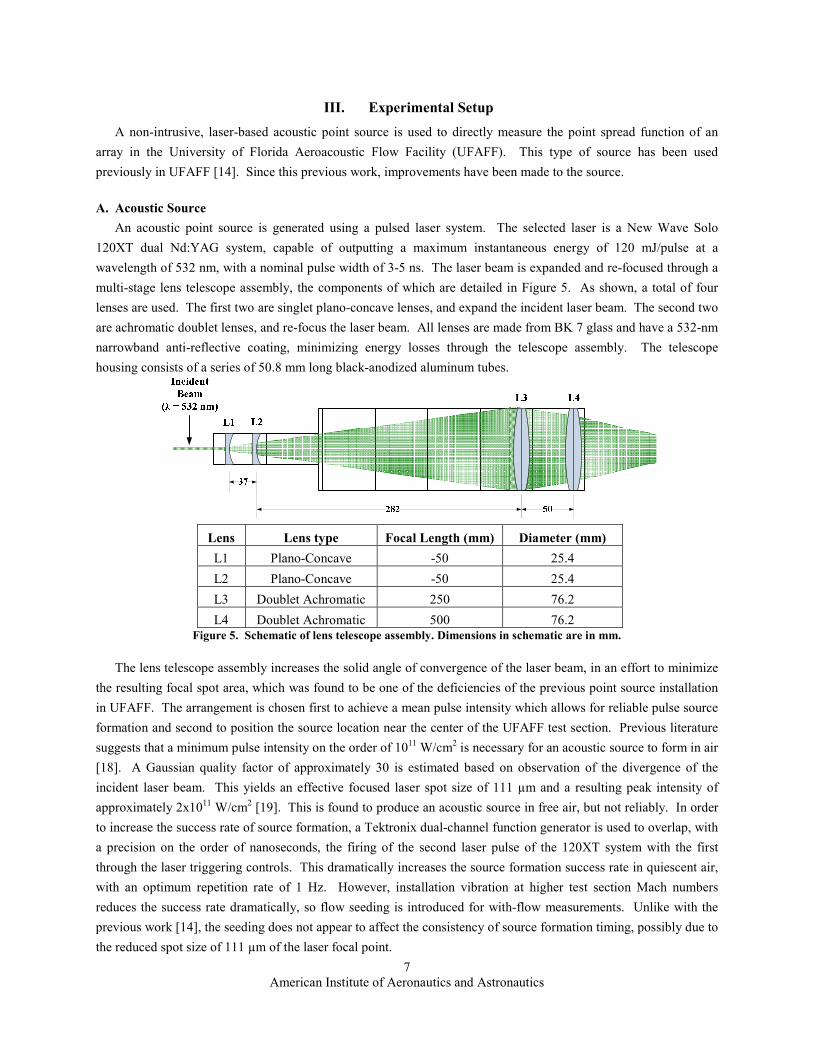
multi-stage lens telescope assembly, the components of which are detailed in Figure 5. As shown, a total of four

lenses are used. The first two are singlet plano-concave lenses, and expand the incident laser beam. The second two

are achromatic doublet lenses, and re-focus the laser beam. All lenses are made from BK 7 glass and have a 532-nm

narrowband anti-reflective coating, minimizing energy losses through the telescope assembly. The telescope

housing consists of a series of 50.8 mm long black-anodized aluminum tubes.

Lens Lens type Focal Length (mm) Diameter (mm)

L1 Plano-Concave -50 25.4

L2 Plano-Concave -50 25.4

L3 Doublet Achromatic 250 76.2

L4 Doublet Achromatic 500 76.2

Figure 5. Schematic of lens telescope assembly. Dimensions in schematic are in mm.

The lens telescope assembly increases the solid angle of convergence of the laser beam, in an effort to minimize

the resulting focal spot area, which was found to be one of the deficiencies of the previous point source installation

in UFAFF. The arrangement is chosen first to achieve a mean pulse intensity which allows for reliable pulse source

formation and second to position the source location near the center of the UFAFF test section. Previous literature

suggests that a minimum pulse intensity on the order of 1011

W/cm2 is necessary for an acoustic source to form in air

[18]. A Gaussian quality factor of approximately 30 is estimated based on observation of the divergence of the

incident laser beam. This yields an effective focused laser spot size of 111 µm and a resulting peak intensity of

approximately 2x1011

W/cm2 [19]. This is found to produce an acoustic source in free air, but not reliably. In order

to increase the success rate of source formation, a Tektronix dual-channel function generator is used to overlap, with

a precision on the order of nanoseconds, the firing of the second laser pulse of the 120XT system with the first

through the laser triggering controls. This dramatically increases the source formation success rate in quiescent air,

with an optimum repetition rate of 1 Hz. However, installation vibration at higher test section Mach numbers

reduces the success rate dramatically, so flow seeding is introduced for with-flow measurements. Unlike with the

previous work [14], the seeding does not appear to affect the consistency of source formation timing, possibly due to

the reduced spot size of 111 µm of the laser focal point.

8


B. Acoustic Instrumentation

A new acoustic array has been designed and fabricated for use with UFAFF [20]. This array frame, shown in

Figure 1, consists of a small-aperture (7.62 cm) array nested in a large-aperture (73.7 cm) array, with a total of 61

microphones present on the array frame. Each array was initially designed as a zero-redundancy multi-arm

logarithmic spiral array [21]. The center reference microphone of the array is a B&K 4954 1/4” free-field

microphone, which has a nominal ±3 dB frequency range of 4 Hz – 100 kHz. The inner two rings of the array are

also each populated with five B&K 4954 microphones. The next three rings of the array are each populated with

five G.R.A.S. 40BE 1/4” microphones, which also have a ±3 dB frequency range of 4 Hz – 100 kHz. These first

five rings define the inner small-aperture array. The remaining seven rings each consist of five B&K 4958 1/4”

microphones with a ±3 dB frequency range of 10 Hz – 20 kHz. These outermost seven rings, along with the

outermost of the three G.R.A.S. rings, define the outer large-aperture array. For all array experiments, all of the

microphones are installed with their protective grids.

While the sampling rate and microphone bandwidth allow for higher-frequency analysis, data are only

considered up to 10 kHz due to scattering effects. As mentioned in Section II, the methods discussed assume a non-

intrusive, or at least correctible, reference microphone measurement. The reference microphone in this case is

within approximately one microphone diameter to the inner array microphones on the array frame, and a significant

scattering effect is noticeable at higher frequencies as shown in subsequent sections. This is verified by subsequent

single free-space microphone measurements. Acoustically absorbent foam is applied to the face of the array to

mitigate this scattering effect, but to simplify analysis and discussion, results are only considered in a band where

scattering is not a problem and acoustic treatment is unnecessary. The array pattern of the outer array is shown in

Figure 2, with example theoretical PSFs at 1 kHz and 10 kHz shown in Figure 3 and Figure 4, respectively.

As a subset of this research, individual free-space measurements are also conducted to evaluate source behavior,

as well as inter-microphone scattering from the inner array microphones to the reference microphone. For these

experiments the array is removed from the facility, and a single microphone located in free space where the array

center reference microphone is normally located, relative to the source. A B&K 4939 1/4” free-field microphone,

with a ±2 dB frequency range of 4 Hz – 100 kHz, is first installed with its protective grid. The grid is then removed

to evaluate grid effects on the observed signal. A B&K 4138 1/8” pressure-field microphone with a ±2 dB

frequency range of 6.5 Hz – 140 kHz is then installed, with grid, in place of the B&K 4939 microphone to evaluate

additional power in the signal beyond 100 kHz. Setup permitting, certain configurations have one or two B&K 4939

reference microphones located equidistant from the acoustic point source, on the opposite side of the test section.

C. Data Acquisition

Data are acquired using an 18-slot National Instruments PXI-1045 chassis. For most experiments, the chassis is

populated with 17 NI PXI-4462 data acquisition (DAQ) cards. Each channel has 24-bit resolution with 118 dB

dynamic range. The first 60 channels are connected to the array microphones. The 61st channel is connected to the

center reference microphone. Depending on configuration, the next one or two channels are occupied by additional

reference microphones. For laser source cases, a Thorlabs DET10A photodetector is connected as the last

acquistion channel to determine the source initiation time and thus acoustic transit times. All acoustic measurements

are ac coupled with a -3 dB cut-on at 3.4 Hz, and appropriate anti-aliasing filters are automatically applied. The

photodetector channel is dc coupled. The sampling rate when using these cards is set to 204,800 samples per

second. All channels are acquired simultaneously.

When acquiring laser pulse data, acquisition is triggered from the output of the laser Q-switch. For each

channel, 6400 samples are acquired, for a resultant block length of 1/32nd

of a second, and 1000 such blocks of data

9


are acquired. Because the Q-switch fires whether or not an acoustic source forms, a block rejection scheme is

necessary in post-processing as described in [14]. Aeroacoustic data are acquired with the same sampling

parameters, but continuously for 30 seconds.

As previously mentioned, source behavior is evaluated using microphones installed in free space for comparison

with the array center reference microphone. As a subset of this work, a high-speed DAQ card is used to investigate

the effects of finite sampling rates on the observed signal. A single, 2-channel 14-bit NI PXI-5122 DAQ card is

installed in the chassis, and connected to either the array center reference microphone or a free-space microphone,

depending on experimental configuration. The photodetector is connected to the second channel. Data are

simultaneously acquired at a sampling rate of 100 megasamples per second. Acoustic channels are ac coupled with

a -3 dB cut-on at 12 Hz. Acquisition is again triggered from the laser Q-switch. System throughput limits the block

length to 1/64th

of a second. As with other laser pulse cases, 1000 blocks are acquired, and a rejection scheme is

necessary to detect blocks where no acoustic source is present.

D. Data Processing

As described in [14], laser pulse data blocks are ensemble averaged in the time domain to reduce the influence of

random electronic and aerodynamic noise. While the block-to-block levels of the acoustic source are observed to

vary, the shape of the wave forms are consistent for a given experiment set, allowing for an average-level signal to

be constructed.

For cases with no flow, a simple level check is applied to each block of data. Background fluctuations are

observed to be on the order of tens of mPa, while peak levels in the laser pulse source range between 20 Pa and 100

Pa with no flow and no seeding. However, for cases with significant flow noise a level check becomes inconsistent.

While visual inspection of blocks shows obvious difference between data without a pulse and data with one, such an

inspection process is intractable for the amount of data acquired. Instead, all of the blocks in the data set are

ensemble averaged. Assuming a 10% success rate for source occurrence (far below that actually realized with

seeding), averaging 1000 blocks of data will yield a reduction in noise levels by 1000, but in signal levels by only

100, yielding an effective boost in signal-to-noise ratio (SNR) of 10. This SNR-boosted waveform is then cross-

correlated with each block of data, and a peak-detection scheme applied to the cross-correlation at time bins near

zero delay. Any block with a peak is retained as having a successful source occurrence, while any without is

rejected.

In our previous research [14], a block rotation scheme was implemented due to small source movement within

the facility. This step is unnecessary for these experiments. While some fluctuation in peak location within a given

data set is observed for significant flow speeds, this fluctuation is found to be independent of whether or not flow

seeding is present, and reduced in scale from the previous work. Photodetector output shows no such fluctuation, so

source initiation time is consistent. It is not known whether the fluctuation is due to actual movement of the source

due to facility vibration, or other flow-based phenomena such as low-frequency unsteadiness in the open jet shear

layer.

A discrete Fourier transform is applied to the sampled data. The nature of the laser pulse source and ensemble-

averaging process assures that the latter portion of each record is zero, so all records can be arbitrarily zero-padded

to achieve a desired narrowband binwidth. In this case the data are padded such that the resultant binwidth is 16 Hz,

for comparison with acquired aeroacoustic data. For the single-microphone signal comparisons, a rectangular

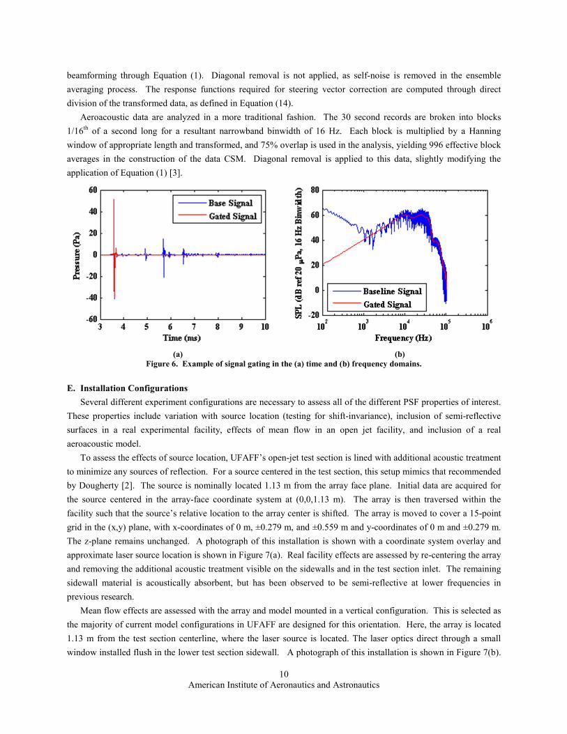
window is applied to gate the initial waveform and isolate it from any reflections. An example of this is shown in

Figure 6. For all other analysis, no window function is applied. All microphone bins for each frequency are stacked

in a vector. The vector is multiplied by its conjugate transpose to build a CSM for that frequency, usable in

10


beamforming through Equation (1). Diagonal removal is not applied, as self-noise is removed in the ensemble

averaging process. The response functions required for steering vector correction are computed through direct

division of the transformed data, as defined in Equation (14).

Aeroacoustic data are analyzed in a more traditional fashion. The 30 second records are broken into blocks

1/16th

of a second long for a resultant narrowband binwidth of 16 Hz. Each block is multiplied by a Hanning

window of appropriate length and transformed, and 75% overlap is used in the analysis, yielding 996 effective block

averages in the construction of the data CSM. Diagonal removal is applied to this data, slightly modifying the

application of Equation (1) [3].

(a)

(b)

Figure 6. Example of signal gating in the (a) time and (b) frequency domains.

E. Installation Configurations

Several different experiment configurations are necessary to assess all of the different PSF properties of interest.

These properties include variation with source location (testing for shift-invariance), inclusion of semi-reflective

surfaces in a real experimental facility, effects of mean flow in an open jet facility, and inclusion of a real

aeroacoustic model.

To assess the effects of source location, UFAFF’s open-jet test section is lined with additional acoustic treatment

to minimize any sources of reflection. For a source centered in the test section, this setup mimics that recommended

by Dougherty [2]. The source is nominally located 1.13 m from the array face plane. Initial data are acquired for

the source centered in the array-face coordinate system at (0,0,1.13 m). The array is then traversed within the

facility such that the source’s relative location to the array center is shifted. The array is moved to cover a 15-point

grid in the (x,y) plane, with x-coordinates of 0 m, ±0.279 m, and ±0.559 m and y-coordinates of 0 m and ±0.279 m.

The z-plane remains unchanged. A photograph of this installation is shown with a coordinate system overlay and

approximate laser source location is shown in Figure 7(a). Real facility effects are assessed by re-centering the array

and removing the additional acoustic treatment visible on the sidewalls and in the test section inlet. The remaining

sidewall material is acoustically absorbent, but has been observed to be semi-reflective at lower frequencies in

previous research.

Mean flow effects are assessed with the array and model mounted in a vertical configuration. This is selected as

the majority of current model configurations in UFAFF are designed for this orientation. Here, the array is located

1.13 m from the test section centerline, where the laser source is located. The laser optics direct through a small

window installed flush in the lower test section sidewall. A photograph of this installation is shown in Figure 7(b).

11


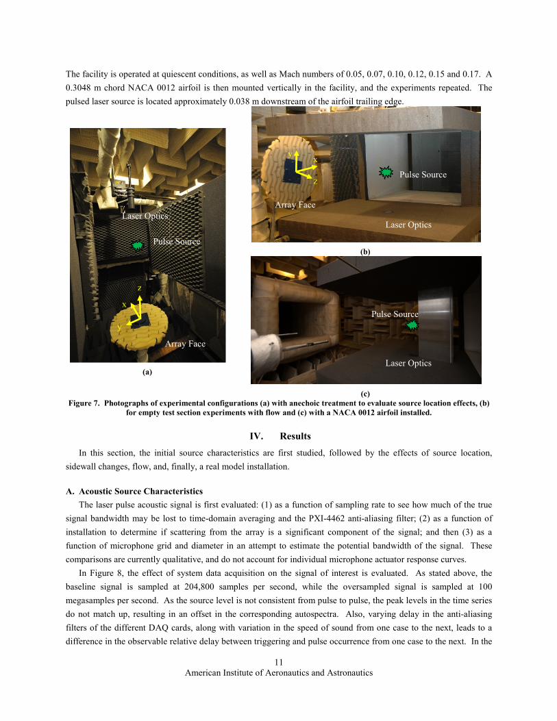
The facility is operated at quiescent conditions, as well as Mach numbers of 0.05, 0.07, 0.10, 0.12, 0.15 and 0.17. A

0.3048 m chord NACA 0012 airfoil is then mounted vertically in the facility, and the experiments repeated. The

pulsed laser source is located approximately 0.038 m downstream of the airfoil trailing edge.

(a)

(b)

(c)

Figure 7. Photographs of experimental configurations (a) with anechoic treatment to evaluate source location effects, (b)

for empty test section experiments with flow and (c) with a NACA 0012 airfoil installed.

IV. Results

In this section, the initial source characteristics are first studied, followed by the effects of source location,

sidewall changes, flow, and, finally, a real model installation.

A. Acoustic Source Characteristics

The laser pulse acoustic signal is first evaluated: (1) as a function of sampling rate to see how much of the true

signal bandwidth may be lost to time-domain averaging and the PXI-4462 anti-aliasing filter; (2) as a function of

installation to determine if scattering from the array is a significant component of the signal; and then (3) as a

function of microphone grid and diameter in an attempt to estimate the potential bandwidth of the signal. These

comparisons are currently qualitative, and do not account for individual microphone actuator response curves.

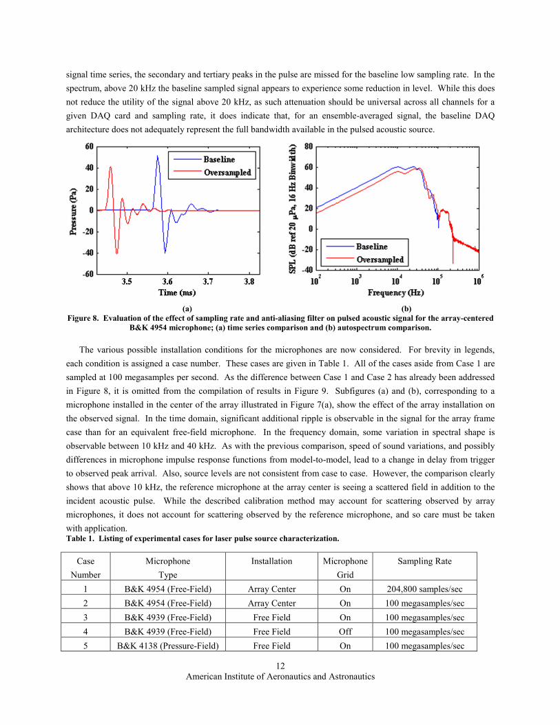
In Figure 8, the effect of system data acquisition on the signal of interest is evaluated. As stated above, the

baseline signal is sampled at 204,800 samples per second, while the oversampled signal is sampled at 100

megasamples per second. As the source level is not consistent from pulse to pulse, the peak levels in the time series

do not match up, resulting in an offset in the corresponding autospectra. Also, varying delay in the anti-aliasing

filters of the different DAQ cards, along with variation in the speed of sound from one case to the next, leads to a

difference in the observable relative delay between triggering and pulse occurrence from one case to the next. In the

x

y

z

Array Face

Pulse Source

Laser Optics Laser Optics

Pulse Source

x y

z

Pulse Source

Laser Optics

Array Face

12


signal time series, the secondary and tertiary peaks in the pulse are missed for the baseline low sampling rate. In the

spectrum, above 20 kHz the baseline sampled signal appears to experience some reduction in level. While this does

not reduce the utility of the signal above 20 kHz, as such attenuation should be universal across all channels for a

given DAQ card and sampling rate, it does indicate that, for an ensemble-averaged signal, the baseline DAQ

architecture does not adequately represent the full bandwidth available in the pulsed acoustic source.

(a)

(b)

Figure 8. Evaluation of the effect of sampling rate and anti-aliasing filter on pulsed acoustic signal for the array-centered

B&K 4954 microphone; (a) time series comparison and (b) autospectrum comparison.

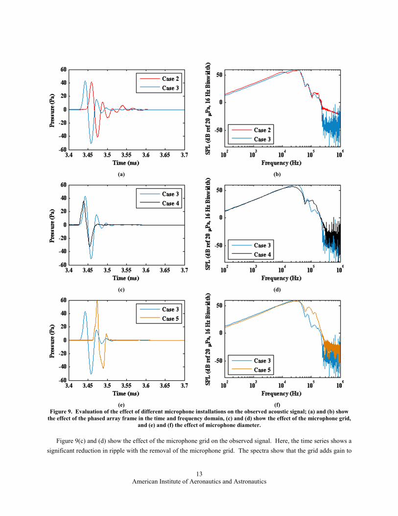
The various possible installation conditions for the microphones are now considered. For brevity in legends,

each condition is assigned a case number. These cases are given in Table 1. All of the cases aside from Case 1 are

sampled at 100 megasamples per second. As the difference between Case 1 and Case 2 has already been addressed

in Figure 8, it is omitted from the compilation of results in Figure 9. Subfigures (a) and (b), corresponding to a

microphone installed in the center of the array illustrated in Figure 7(a), show the effect of the array installation on

the observed signal. In the time domain, significant additional ripple is observable in the signal for the array frame

case than for an equivalent free-field microphone. In the frequency domain, some variation in spectral shape is

observable between 10 kHz and 40 kHz. As with the previous comparison, speed of sound variations, and possibly

differences in microphone impulse response functions from model-to-model, lead to a change in delay from trigger

to observed peak arrival. Also, source levels are not consistent from case to case. However, the comparison clearly

shows that above 10 kHz, the reference microphone at the array center is seeing a scattered field in addition to the

incident acoustic pulse. While the described calibration method may account for scattering observed by array

microphones, it does not account for scattering observed by the reference microphone, and so care must be taken

with application. Table 1. Listing of experimental cases for laser pulse source characterization.

Case

Number

Microphone

Type

Installation Microphone

Grid

Sampling Rate

1 B&K 4954 (Free-Field) Array Center On 204,800 samples/sec

2 B&K 4954 (Free-Field) Array Center On 100 megasamples/sec

3 B&K 4939 (Free-Field) Free Field On 100 megasamples/sec

4 B&K 4939 (Free-Field) Free Field Off 100 megasamples/sec

5 B&K 4138 (Pressure-Field) Free Field On 100 megasamples/sec

13


(a)

(b)

(c)

(d)

(e)

(f)

Figure 9. Evaluation of the effect of different microphone installations on the observed acoustic signal; (a) and (b) show

the effect of the phased array frame in the time and frequency domain, (c) and (d) show the effect of the microphone grid,

and (e) and (f) the effect of microphone diameter.

Figure 9(c) and (d) show the effect of the microphone grid on the observed signal. Here, the time series shows a

significant reduction in ripple with the removal of the microphone grid. The spectra show that the grid adds gain to

14


the acoustic signal in a band from below 20 kHz up to 80 kHz, as expected from the grid correction data available

from B&K. However, the grid appears to significantly attenuate the signal upwards of 80 kHz.

Figure 9 (e) and (f) qualitatively show the effect of microphone size (and bandwidth) on the observed signal.

This comparison is qualitative since free-field microphones include additional damping in the diaphragm response to

compensate for free-field scattering, while pressure-field microphones do not [22]. This means that the expected

observed output from a B&K 4138 microphone should already show additional gain at high frequencies compared to

a B&K 4939 microphone, signal bandwidth aside. Nevertheless, the gain shown in the frequency domain of

multiple orders of magnitude by using the smaller microphone is beyond any expected correction factor.

Additionally, the sharpening of the initial peak in the time domain is indicative that the true signal bandwidth is well

beyond that observable by a B&K 4939 or B&K 4138 microphone. The net result of this analysis shows that, while

levels from experiment to experiment may not be completely repeatable, the pulsed laser source provides a high

bandwidth signal with a consistent waveform shape (for a given physical installation), suitable for high frequency

applications where precise phase information is desired.

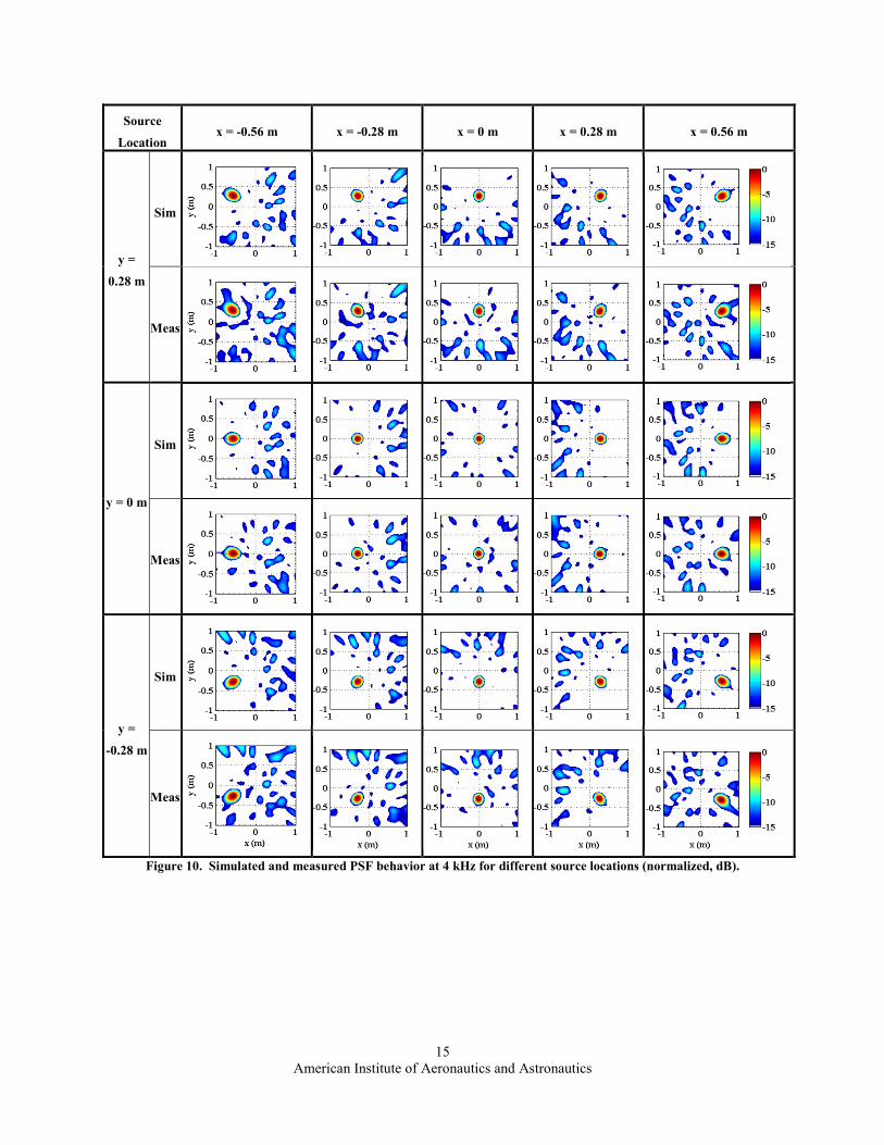
B. PSF as a Function of Source Location

The array response in a clean acoustic installation, as shown in Figure 7(a), is now considered. The experimental

PSFs are compared to theoretical PSFs for equivalent source locations. For this and all subsequent analyses, the

discussion is limited to a case of 4 kHz. This frequency is selected as it is within a band unaffected by reference

microphone scattering while having a small beamwidth given the installation dimensions of interest, while, for the

NACA 0012 case, providing a data set where the airfoil trailing edge noise is dominant. All PSF plots are shown in

a scale of dB normalized to peak levels.

The predicted and experimental PSF behaviors are shown in Figure 10. In all figures, the plotted coordinates

correspond to those shown in the appropriate installation coordinate systems of Figure 7. Predicted PSFs are

generated by simulating a monopole source at the desired location in space with a free-field propagation model,

from Equation (12), for the array’s design microphone coordinates. Both the simulated and experimental data are

processed through Equation (1). For both cases, the PSFs are clearly not shift-invariant for these source-array

combinations, as expected since source displacements within the scan plane are on the order of the array-to-scan-

plane distance. The overall behaviors of both are also similar, with regard to the displacement and distortion of the

main lobe. However, specific details of the experimental data differ from the predictions. The shape of the

experimental main lobes shows some additional asymmetry as compared to the theoretical responses. Sidelobe

distributions also differ for each case.

C. Minor Reflective Source

The next case considered involves the removal of the additional acoustic treatment, as shown in Figure 7(a),

lining the facility. The resultant test section configuration matches a more realistic installation, where only acoustic

foam sidewalls are present similar to that shown in Figure 7(b), although still in a flyover configuration. Resultant

beam maps for the theoretical free-space PSF and the measured PSF are shown in Figure 11. The sidewalls are

illustrated in the figure, along with the contraction entrance into the facility. While the results do not show a perfect

image source, the upper sidelobe is accentuated to a level beyond that visible for an equivalent experimental source-

array configuration from Figure 10. This may be due to a mild reflection, indicating that, at 4 kHz, the facility does

have some reflective behavior, which is also asymmetric.

15


Source

Location x = -0.56 m x = -0.28 m x = 0 m x = 0.28 m x = 0.56 m

y =

0.28 m

Sim

Meas

y = 0 m

Sim

Meas

y =

-0.28 m

Sim

Meas

Figure 10. Simulated and measured PSF behavior at 4 kHz for different source locations (normalized, dB).

16


(a)

(b)

Figure 11. Comparison of (a) ideal free-space and (b) measured PSF at 4 kHz for standard UFAFF configuration.

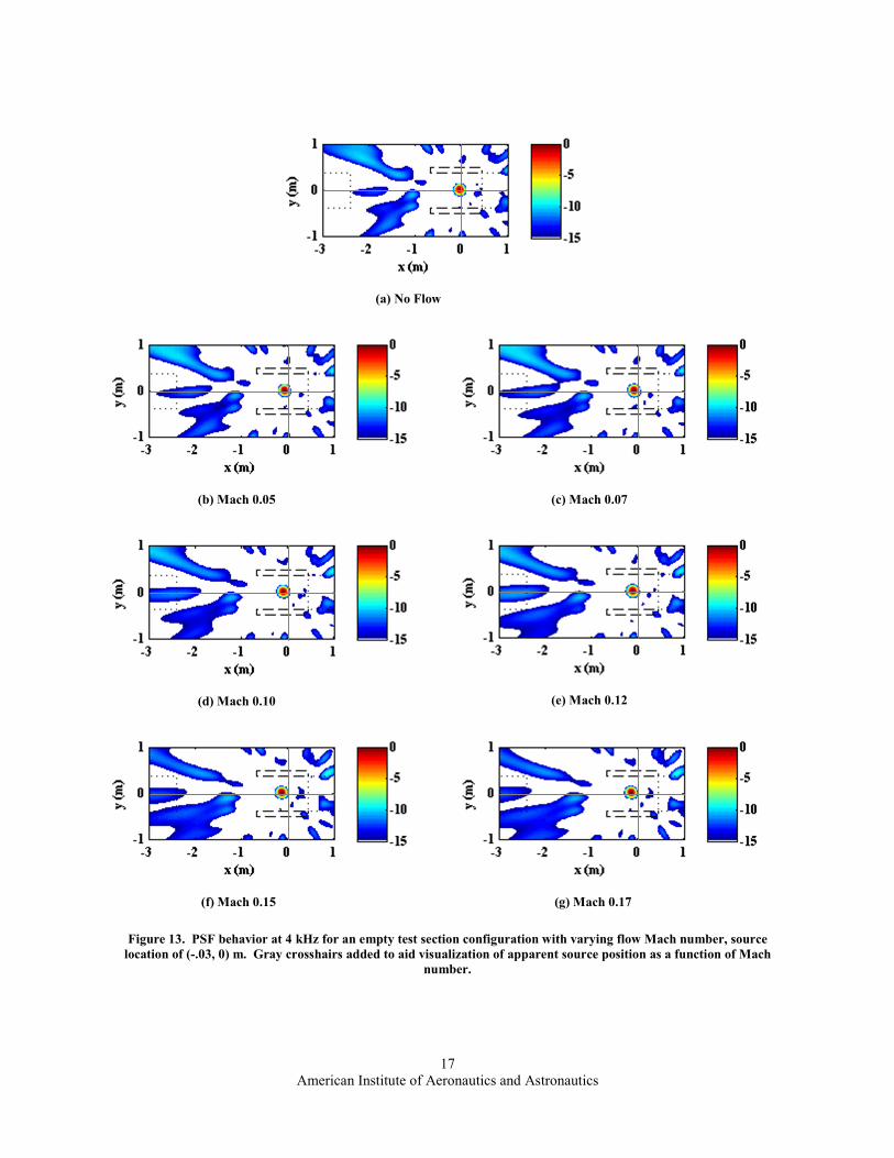
D. Sideline Configurations – Effects of Flow and Model Installation

The facility is reconfigured to a sideline installation as discussed previously. A legend of the symbols present on

the beam maps is shown in Figure 12, to identify the overlays of sidewalls, the facility inlet, the test section jet

collector and the NACA 0012 model. Previous research [14] has shown that Amiet’s shear layer correction properly

shifts data in UFAFF under regular, simple conditions such as these. As such, theoretical PSFs are not shown.

Instead, PSF behavior in an empty test section is shown, followed by behavior with the NACA 0012 model.

Figure 12. Legend of symbols used in sideline beam maps.

Acoustic Foam

Sidewall

Inlet

Inlet

Acoustic Foam

Sidewall

NACA 0012

Airfoil Test Section

Jet Collector

Flow Direction

17


(a) No Flow

(b) Mach 0.05

(c) Mach 0.07

(d) Mach 0.10

(e) Mach 0.12

(f) Mach 0.15

(g) Mach 0.17

Figure 13. PSF behavior at 4 kHz for an empty test section configuration with varying flow Mach number, source

location of (-.03, 0) m. Gray crosshairs added to aid visualization of apparent source position as a function of Mach

number.

18


(a) No Flow

(b) Mach 0.05

(c) Mach 0.07

(d) Mach 0.10

(e) Mach 0.12

(f) Mach 0.15

(g) Mach 0.17

Figure 14. PSF behavior at 4 kHz for a NACA 0012 test section configuration (0° AoA) with varying flow Mach number,

source location of (-.03, 0) m. Gray crosshairs added to aid visualization of apparent source position as a function of

Mach number.

19


Figure 13 shows the PSF as a function of Mach number for the empty test section configuration shown in Figure

7(b). Figure 14 shows the PSF as a function of Mach number for the airfoil configuration shown in Figure 7(c).

Both of these cases show extremely similar behavior. The array PSF, while slightly skewed, appears to have a Mach

number invariant shape. Also, no reflections are visible from the sidewalls, inlet or jet collector assemblies. Of

note, the apparent source location is ~0.04 m higher along the y-axis than the true source location. This is indicative

of array misalignment in the experiment.

Misalignment aside, these results raise the question as to why such measurements may be necessary for these

experiments, as opposed to using a free-space steering vector and simply applying Amiet’s correction. The answer

to this comes from the response functions computed in Section II. For a true, free-space source, the phase of the

response function between the reference microphone and any array microphone should be linear as a function of

frequency, representing an ideal delay. As Amiet’s method simply modifies the delay, the modified response

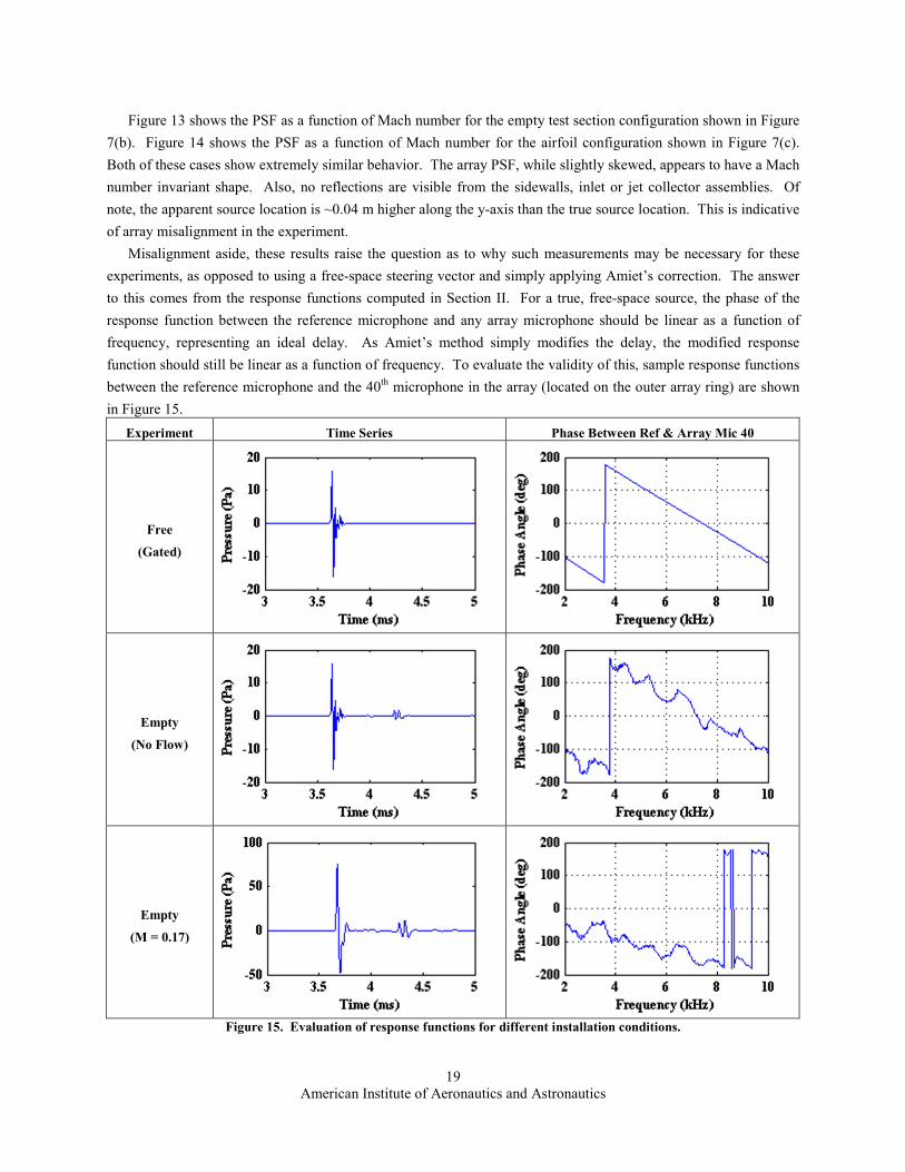
function should still be linear as a function of frequency. To evaluate the validity of this, sample response functions

between the reference microphone and the 40th

microphone in the array (located on the outer array ring) are shown

in Figure 15.

Experiment Time Series Phase Between Ref & Array Mic 40

Free

(Gated)

Empty

(No Flow)

Empty

(M = 0.17)

Figure 15. Evaluation of response functions for different installation conditions.

20


From these plots, it is clear that while the clean signal does show a linear phase response, the experimental

conditions for the real facility without and with flow do not. The secondary structure in the second and third time

series corresponds to the appropriate delay time for a reflection from the acoustic foam sidewalls. While the

reflections seen in the time series do not manifest as noticeable sources in previously-evaluated beam maps, they do

appear to have a significant effect on the phase behavior between microphones. The deviation in these phase plots

could lead to serious errors in levels computed from beamformer outputs, and would not be accounted for using a

simple shear layer correction method with a free-space steering vector.

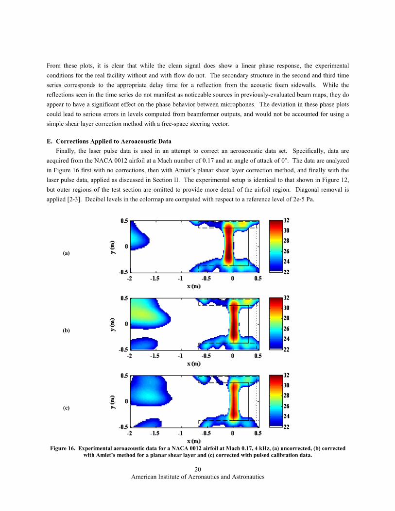
E. Corrections Applied to Aeroacoustic Data

Finally, the laser pulse data is used in an attempt to correct an aeroacoustic data set. Specifically, data are

acquired from the NACA 0012 airfoil at a Mach number of 0.17 and an angle of attack of 0°. The data are analyzed

in Figure 16 first with no corrections, then with Amiet’s planar shear layer correction method, and finally with the

laser pulse data, applied as discussed in Section II. The experimental setup is identical to that shown in Figure 12,

but outer regions of the test section are omitted to provide more detail of the airfoil region. Diagonal removal is

applied [2-3]. Decibel levels in the colormap are computed with respect to a reference level of 2e-5 Pa.

(a)

(b)

(c)

Figure 16. Experimental aeroacoustic data for a NACA 0012 airfoil at Mach 0.17, 4 kHz, (a) uncorrected, (b) corrected

with Amiet’s method for a planar shear layer and (c) corrected with pulsed calibration data.

21


The baseline, uncorrected case in subfigure (a) shows the expected behavior for this flow condition, given a

misaligned array which leads to a vertical offset in the beam map. The trailing edge noise source is dominant, but is

shifted downstream in the beam map. Amiet’s correction method, (b), restores it to the vicinity of the trailing edge.

However, Amiet’s method does nothing with regard to the noise sources along the sidewalls, whether they be

scrubbing noise, sidelobes, or out-of-plane noise sources. It also does not account for the array misalignment.

Furthermore, it enhances the downstream sidelobe. The experimentally-corrected steering vectors, like Amiet’s

correction method, properly restore the trailing edge noise source to the model trailing edge, and corrects for the

apparent alignment issue. However, the method shown in (c) does so with less enhancement of the downstream

sidelobe, and actually shows mitigation of the extraneous sources along the test section sidewall. Additionally, the

experimental correction method appears to sharpen the trailing edge noise source in the beam map as compared to

the Amiet-corrected and uncorrected data. Overall level ranges within the subfigures are all of similar scale.

V. Conclusions and Future Work

A non-intrusive point source is used to measure the PSF of a broadband, aeroacoustic phased microphone array

under varying experimental conditions. To generate the source, a Nd:YAG laser is focused to a point in space and

pulsed at 1 Hz. The repetitive acoustic source is high bandwidth and consistent in waveform shape, although overall

pulsed levels vary from block to block. Signals are ensemble-averaged to focus on the deterministic, periodic laser

pulsing and reject background and model flow noise. Facility conditions are varied from an anechoic-like treatment

to a true experimental configuration with an airfoil model and low Mach number flow.

The results shown indicate that the pulsed laser source is a valid way to measure an array’s PSF. The source has

sufficient bandwidth to cover the entire acoustic measurement range of interest and allows for characterization of

installation realities, such as microphone-array-frame scattering, which may not otherwise be accounted for in an

experiment. Under clean conditions, the beamwidth of the experimental data matches the design beamwidth of the

array for a given frequency. Sidelobe distributions differ, but not by a significant amount in most cases considered

to date, and may be due to errors in microphone locations. The measurement method is capable of detecting partial

reflections in a given configuration. Also, it provides an alternative to applying a shear layer correction technique,

at least for near shift-invariant measurement conditions, when a mean shear layer is present in an open jet

measurement configuration.

Subsequent work will involve additional investigation of coherent reflection characteristics with various

boundary conditions more closely approaching a hard-walled boundary condition. Also, additional aeroacoustic

measurements should be considered where the region of interest is no longer shift-invariant, such that a shift-based

correction can be compared with an Amiet-based correction. The effect of the correction method on integrated level

uncertainties must be considered, as well as direct incorporation into deconvolution beamforming.

Acknowledgements

The authors acknowledge the financial support provided by the Florida Center for Advanced Aero-Propulsion.

22


References

[1] D.H. Johnson and D.E. Dudgeon, Array Signal Processing: Concepts and Techniques, Prentice Hall, 1993.

[2] R.P. Dougherty, “Beamforming in Acoustic Testing,” in Aeroacoustic Measurements, T.J. Mueller, Ed.,

Springer-Verlag, Berlin, Heidelberg & New York, 2002.

[3] T.F. Brooks and W.M. Humphreys, “A Deconvolution Approach for the Mapping of Acoustic Sources

(DAMAS) Determined from Phased Microphone Arrays,” Journal of Sound and Vibration, Vol. 294, pp. 856-879,

2006.

[4] R.P. Dougherty, “Extensions of DAMAS and Benefits and Limitations of Deconvolution in Beamforming,”

AIAA Paper 2005-2961, 11th

AIAA/CEAS Aeroacoustics Conference, Monterey, CA, May 2005.

[5] K. Ehrenfried and L. Koop, “Comparison of Iterative Deconvolution Algorithms for the Mapping of

Acoustic Sources,” AIAA Journal, Vol. 45, No. 7, pp. 1584-1595, 2007.

[6] P. Sijtsma, “CLEAN Based on Spatial Source Coherence,” International Journal of Aeroacoustics, Vol. 6,

No. 4, pp. 357-374, 2007.

[7] T. Yardibi, J. Li, P. Stoica, L. Cattafesta III, “Sparsity Constrained Deconvolution Approaches for Acoustic

Source Mapping,” Journal of the Acoustical Society of America, Vol. 123, No. 5, pp. 2631-2642, 2008.

[8] P.A. Ravetta, R.A. Burdisso and W.F. Ng, “Noise Source Localization and Optimization of Phased-Array

Results”, AIAA Journal, Vol. 47, No. 11, pp. 2520-2533, 2009.

[9] T. Yardibi, J. Li, P. Stoica, N. Zawodny and L. Cattafesta III, “A Covariance-Fitting Approach for

Correlated Acoustic Source Mapping,” Journal of the Acoustical Society of America, Vol. 127, No. 5, pp. 2920-

2931, 2010.

[10] T. Suzuki, “DAMAS2 Using a Point-Spread Function Weakly Varying in Space,” AIAA Journal, Vol. 48,

No. 9, pp. 2165-2169, 2010.

[11] W.M. Humphreys, T.F. Brooks, W.W. Hunter Jr. and K.R. Meadows, “Design and Use of Microphone

Directional Arrays for Aeroacoustic Measurements,” AIAA Paper 98-0471, 36th AIAA Aerospace Sciences

Meeting & Exhibit, Reno, NV, January 1998.

[12] S. Oerlemans and P. Sijtsma, “Effects of Wind Tunnel Side-Plates on Airframe Noise Measurements with

Phased Arrays,” NLR-TP-2000-169, 2000.

[13] B.A. Fenech and K. Takeda, “Toward More Accurate Beamforming Levels in Closed-Section Wind

Tunnels via De-Reverberation,” AIAA Paper 2007-3431, 13th

AIAA/CEAS Aeroacoustics Conference, Rome, May

2007.

[14] C. Bahr, N. Zawodny, T. Yardibi, F. Liu, D. Wetzel, B. Bertolucci and L. Cattafesta III, “Shear Layer

Time-Delay Correction using a Non-Intrusive Acoustic Point Source,” International Journal of Aeroacoustics, to

appear, 2010.

[15] T. Yardibi, C. Bahr, N. Zawodny, F. Liu, L. Cattafesta III and J. Li, “Uncertainty Analysis of the Standard

Delay-and-Sum Beamformer and Array Calibration,” Journal of Sound and Vibration, Vol. 329, pp. 2654-2682,

2010.

[16] T.F. Brooks, W.M. Humphreys and G.E. Plassman, “DAMAS Processing for a Phased Array Study in the

NASA Langley Jet Noise Laboratory,” AIAA Paper 2010-3780, 16th AIAA/CEAS Aeroacoustics Conference,

Stockholm, Sweden, June 2010.

[17] D.T. Blackstock, “Spherical Waves,” Fundamentals of Physical Acoustics, John Wiley and Sons, Inc., New

York, 2000.

[18] Q. Qin and K. Attenborough, “Characteristics and Application of Laser-Generated Acoustic Shock Waves

in Air,” Applied Acoustics, Vol. 65, pp. 325-240, 2004.

23


[19] CVI Melles Griot, “Gaussian Beam Optics,”

https://cvimellesgriot.com/Products/Documents/TechnicalGuide/Gaussian-Beam-Optics.pdf, (last accessed April

2011), 2009.

[20] D. Wetzel, “An Experimental Investigation of Circulation Control Acoustics,” Ph.D. Dissertation,

Mechanical and Aerospace Engineering, University of Florida, 2011.

[21] J.R. Underbrink, “Practical Considerations in Focused Array Design for Passive Broad-Band Source

Mapping Applications,” M.S. Thesis, Acoustics Dept., The Pennsylvania State University, State College, PA, 1995.

[22] Bruel & Kjær, “Chapter 2: Microphone Theory,” Microphone Handbook Vol. 1: Theory, BE 1447-11,

Nærum, Denmark, July 1996.