measure and integration · originally, measure theory was the theory of the lebesgue measure, and...

Chapter 5

Measure and integration

In calculus you have learned how to calculate the size of different kinds ofsets: the length of a curve, the area of a region or a surface, the volume ormass of a solid. In probability theory and statistics you have learned how tocompute the size of other kinds of sets: the probability that certain eventshappen or do not happen.

In this chapter we shall develop a general theory for the size of sets,a theory that covers all the examples above and many more. Just as theconcept of a metric space gave us a general setting for discussing the notionof distance, the concept of a measure space will provide us with a generalsetting for discussing the notion of size.

In calculus we use integration to calculate the size of sets. In this chap-ter we turn the situation around: We first develop a theory of size andthen use it to define integrals of a new and more general kind. As we shallsometimes wish to compare the two theories, we shall refer to integrationas taught in calculus as Riemann-integration in honor of the German math-ematician Bernhard Riemann (1826-1866) and the new theory developedhere as Lebesgue integration in honor of the French mathematician HenriLebesgue (1875-1941).

Let us begin by taking a look at what we might wish for in a theory ofsize. Assume what we want to measure the size of subsets of a set X (ifyou need something concrete to concentrate on, you may let X = R2 andthink of the area of subsets of R2, or let X = R3 and think of the volume ofsubsets of R3). What properties do we want such a measure to have?

Well, if µ(A) denotes the size of a subset A of X, we would expect

(i) µ(∅) = 0

as nothing can be smaller than the empty set. In addition, it seems reason-able to expect:

1

2 CHAPTER 5. MEASURE AND INTEGRATION

(ii) If A1, A2, A3 . . . is a disjoint sequence of sets, then

µ(⋃n∈N

An) =∞∑

n=1

µ(An)

These two conditions are, in fact, all we need to develop a reasonabletheory of size, except for one complication: It turns out that we can not ingeneral expect to measure the size of all subsets of X – some subsets arejust so irregular that we can not assign a size to them in a meaningful way.This means that before we impose conditions (i) and (ii) above, we need todecide which properties the measurable sets (those we are able to assign asize to) should have. If we call the collection of all measurable sets A, thestatement A ∈ A is just a shorthand for “A is measurable”.

The first condition is simple; since we have already agreed that µ(∅) = 0,we must surely want to impose

(iii) ∅ ∈ A

For the next condition, assume that A ∈ A. Intuitively, this means thatwe should be able to assign a size µ(A) to A. If the size µ(X) of the entirespace is finite, we ought to have µ(Ac) = µ(X)−µ(A), and hence Ac shouldbe measurable. We shall impose this condition even when X has infinitesize:

(iv) If A ∈ A, then Ac ∈ A.

For the third and last condition, assume that An is a sequence ofdisjoint sets in A. In view of condition (ii), it is natural to assume that⋃

n∈N An is in A. We shall impose this condition even when the sequence isnot disjoint (there are arguments for this that I don’t want to get involvedin at the moment):

(v) If Ann∈N is a sequence of sets in A, then⋃

n∈N An ∈ A.

When we now begin to develop the theory systematically, we shall takethe five conditions above as our starting point.

5.1 Measure spaces

Assume that X is a nonempty set. A collection A of subsets of X thatsatisfies conditions (iii)-(v) above, is called a σ-algebra. More succinctly:

Definition 5.1.1 Assume that X is a nonempty set. A collection A ofsubsets of X is called a σ-algebra if the following conditions are satisfied:

5.1. MEASURE SPACES 3

(i) ∅ ∈ A

(ii) If A ∈ A, then Ac ∈ A.

(ii) If Ann∈N is a sequence of sets in A, then⋃

n∈N An ∈ A.

If A is a σ-algebra of subsets of X, we call the pair (X,A) a measurablespace.

As already mentioned, the intuitive idea is that the sets in A are those thatare so regular that we can measure their size.

Before we introduce measures, we take a look at some simple conse-quences of the definition above:

Proposition 5.1.2 Assume that A is a σ-algebra on X. Then

a) X ∈ A.

b) If Ann∈N is a sequence of sets in A, then⋂

n∈N An ∈ A.

c) If A1, A2, . . . , An ∈ A, then A1∪A2∪ . . .∪An ∈ A and A1∩A2∩ . . .∩An ∈ A.

d) If A,B ∈ A, then A \B ∈ A.

Proof: a) By conditions (i) and (ii) in the definition, X = ∅c ∈ A.

b) By condition (ii), each Acn is in A, and hence

⋃n∈N Ac

n ∈ A by condi-tion (iii). By one of De Morgan’s laws,( ⋂

n∈NAn

)c =⋃n∈N

Acn

and hence(⋂

n∈N An

)c is in A. Using condition (ii) again, we see that⋂n∈N An is in A.

c) If we extend the finite sequence A1, A2, . . . , An to an infinite oneA1, A2, . . . , An, ∅, ∅, . . ., we see that

A1 ∪A2 ∪ . . . ∪An =⋃n∈N

An ∈ A

by condition (iii). A similar trick works for intersections, but we have toextend the sequence A1, A2, . . . , An to A1, A2, . . . , An, X,X, . . . instead ofA1, A2, . . . , An, ∅, ∅, . . .. The details are left to the reader.

d) We have A\B = A∩Bc, which is inA by condition (ii) and c) above. 2


It is time to turn to measures. Before we look at the definition, there isa small detail we have to take care of. As you know from calculus, there aresets of infinite size – curves of infinite length, surfaces of infinite area, solidsof infinite volume. We shall use the symbol ∞ to indicate that sets haveinfinite size. This does not mean that we think of ∞ as a number; it is justa symbol to indicate that something has size bigger than can be specifiedby a number.

A measure µ assigns a value µ(A) (“the size of A”) to each set A in theσ-algebra A. The value is either ∞ or a nonnegative number. If we let

R+ = [0,∞) ∪ ∞

be the set of extended, nonnegative real numbers, µ is a function from A toR+. In addition, µ has to satisfy conditions (i) and (ii) above, i.e.:

Definition 5.1.3 Assume that (X,A) is a measurable space. A measureon (X,A) is a function µ : A → R+ such that

(i) µ(∅) = 0

(ii) (Countable additivity) If A1, A2, A3 . . . is a disjoint sequence of setsfrom A, then

µ(∞⋃

n=1

AN ) =∞∑

n=1

µ(An)

The triple (X,A, µ) is then called a measure space.

Let us take a look at some examples.

Example 1: Let X = x1, x2, . . . , xn be a finite set, and let A be thecollection of all subsets of X. For each set A ⊂ X, let

µ(A) = |A| = the number of elements in A

Then µ is called the counting measure on X, and (X,A, µ) is a measurespace. ♣

The next two examples show two simple modifications of counting mea-sures.

Example 2: Let X and A be as in Example 1. For each element x ∈ X,let m(x) be a nonnegative, real number (the weight of x). For A ⊂ X, let

µ(A) =∑x∈A

mx


Then (X,A, µ) is a measure space. ♣

Example 3: Let X = x1, x2, . . . , xn, . . . be a countable set, and let A bethe collection of all subsets of X. For each set A ⊂ X, let

µ(A) = the number of elements in A

where we put µ(A) = ∞ if A has infinitely many elements. Again µ is calledthe counting measure on X, and (X,A, µ) is a measure space. ♣

The next example is also important, but rather special.

Example 4: Let X be a any set, and let A be the collection of all subsetsof X. Choose an element a ∈ X, and define

µ(A) =

1 if a ∈ A

0 if a /∈ A

Then (X,A, µ) is a measure space, and µ is called the point measure at a. ♣

The examples we have looked at so far are important special cases, butrather untypical of the theory – they are too simple to really need the fullpower of measure theory. The next examples are much more typical, but atthis stage we can not define them precisely, only give an intuitive descriptionof their most important properties.

Example 5: In this example X = R, A is a σ-algebra containing all openand closed sets (we shall describe it more precisely later), and µ is a measureon (X,A) such that

µ([a, b]) = b− a

whenever a ≤ b. This measure is called the Lebesgue measure on R, and wecan think of it as an extension of the notion of length to more general sets.The sets in A are those that can be assigned a generalized “length” µ(A) ina systematic way. ♣

Originally, measure theory was the theory of the Lebesgue measure, andit remains one of the most important examples. It is not at all obvious thatsuch a measure exists, and one of our main tasks later in the next chapterwill be to show that it does.

Lebesgue measure can be extended to higher dimensions:

Example 6: In this example X = R2, A is a σ-algebra containing all openand closed sets, and µ is a measure on (X,A) such that

µ([a, b]× [c, d]) = (b− a)(d− c)


whenever a ≤ b and c ≤ d (this just means that the measure of a rectangleequals its area). This measure is called the Lebesgue measure on R2, and wecan think of it as an extension of the notion of area to more general sets.The sets in A are those that can be assigned a generalized “area” µ(A) in asystematic way.

There are obvious extensions of this example to higher dimensions: Thethree dimensional Lebesgue measure assigns value

µ([a, b]× [c, d]× [e, f ]) = (b− a)(d− c)(f − e)

to all rectangular boxes and is a generalization of the notion of volume. Then-dimensional Lebesgue measure assigns value

µ([a1, b1]× [a2, b2]× · · · × [an, bn]) = (b1 − a1)(b2 − a2) · . . . · (bn − an)

to all n-dimensional, rectangular boxes and represents n-dimensional vol-ume. ♣

Although we have not yet constructed the Lebesgue measures, we shallfeel free to use them in examples and exercises. Let us finally take a look attwo examples from probabilty theory.

Example 7: Assume we want to study coin tossing, and that we plan totoss the coin N times. If we let H denote “heads” and T “tails”, the possibleoutcomes can be represented as all sequences of H’s and T’s of length N . Ifthe coin is fair, all such sequences have probability 1

2n .To fit this into the framework of measure theory, let X be the set of all

sequences of H’s and T’s of length N , let A be the collection of all subsetsof X, and let µ be given by

µ(A) =|A|2n

where |A| is the number of elements in A. Hence µ is the probability of theevent A. It is easy to check that µ is a measure on (X,A). ♣

In probability theory it is usual to call the underlying space Ω (instead ofX) and the measure P (instead of µ), and we shall often refer to probabilityspaces as (Ω,A, P ).

Example 8: We are still studying coin tosses, but this time we don’t knowbeforehand how many tosses we are going to make, and hence we have toconsider all sequences of H’s and T’s of infinite length, that is all sequences

ω = ω1, ω2, ω3, . . . , ωn, . . .


where each ωi is either H or T. We let Ω be the collection of all such se-quences.

To describe the σ-algebra and the measure, we first need to introducethe so-called cylinder sets: If a = a1, a2, . . . , an is a finite sequence of H’sand T’s, we let

Ca = ω ∈ Ω |ω1 = a1, ω2 = a2, . . . , ωn = an

and call it the cylinder set generated by a. Note that Ca consists of allsequences of coin tosses beginning with the sequence a1, a2, . . . , an. Sincethe probability of starting a sequence of coin tosses with a1, a2, . . . , an is 1

2n ,we want a measure such that P (Ca) = 1

2n .The measure space (Ω,A, P ) of infinite coin tossing consists of Ω, a σ-

algebraA containing all cylinder sets, and a measure P such that P (Ca) = 12n

for all cylinder sets of length n. It is not at all obvious that such a measurespace exists, but it does (as we shall prove in the next chapter), and it isthe right setting for the study of coin tossing of unrestricted length. ♣

Let us return to Definition 5.1.3 and derive some simple, but extremelyuseful consequences. Note that all these properties are properties we wouldexpect of a measure.

Proposition 5.1.4 Assume that (X,A, µ) is a measure space.

a) (Finite additivity) If A1, A2, . . . , Am are disjoint sets in A, then

µ(A1 ∪A2 ∪ . . . ∪Am) = µ(A1) + µ(A2) + . . . + µ(Am)

b) (Monotonicity) If A,B ∈ A and B ⊂ A, then µ(B) ≤ µ(A).

c) If A,B ∈ A, B ⊂ A, and µ(A) < ∞, then µ(A \B) = µ(A)− µ(B).

d) (Countable subadditivity) If A1, A2, . . . , An, . . . is a (not necessarilydisjoint) sequence of sets from A, then

µ(⋃n∈N

An) ≤∞∑

n=1

µ(An)

Proof: a) We fill out the the sequence with empty sets to get an infinitesequence

A1, A2, . . . , Am, Am+1, Am+2 . . .

where An = ∅ for n > m. Then clearly

µ(A1∪A2∪. . .∪Am) = µ(⋃n∈N

An) =∞∑

n=1

µ(An) = µ(A1)+µ(A2)+. . .+µ(An)


where we have used the two parts of definition 5.1.3.

b) We write A = B ∪ (A \ B). By Proposition 5.1.2d), A \ B ∈ A, andhence by part a) above

µ(A) = µ(B) + µ(A \B) ≥ µ(B)

c) By the argument in part b),

µ(A) = µ(B) + µ(A \B)

Since µ(A) is finite, so is µ(B), and we may subtract µ(B) on both sides ofthe equation to get the result.

d) Define a new, disjoint sequence of sets B1, B2, . . . by:

B1 = A1, B2 = A2\A1, B3 = A3\(A1∪A2), B4 = A4\(A1∪A2∪A3), . . .

Note that⋃

n∈N Bn =⋃

n∈N An (make a drawing). Hence

µ(⋃n∈N

An) = µ(⋃n∈N

Bn) =∞∑

n=1

µ(Bn) ≤∞∑

n=1

µ(An)

where we have applied part (ii) of Definition 5.1.3 to the disjoint sequenceBn and in addition used that µ(Bn) ≤ µ(An) by part b) above. 2

The next properties are a little more complicated, but not unexpected.They are often referred to as continuity of measures:

Proposition 5.1.5 Let Ann∈N be a sequence of measurable sets in a mea-sure space (X,A, µ).

a) If the sequence is increasing (i.e. An ⊂ An+1 for all n), then

µ(⋃n∈N

An) = limn→∞

µ(An)

b) If the sequence is decreasing (i.e. An ⊃ An+1 for all n), and µ(A1) isfinite, then

µ(⋂n∈N

An) = limn→∞

µ(An)

Proof: a) If we put E1 = A1 and En = An \ An−1 for n> 1, the sequenceEn is disjoint, and

⋃nk=1 Ek = An for all N (make a drawing). Hence

µ(⋃n∈N

An) = µ(⋃n∈N

En) =∞∑

n=1

µ(En) =


= limn→∞

n∑k=1

µ(Ek) = limn→∞

µ(n⋃

k=1

Ek) = limn→∞

µ(An)

where we have used the additivity of µ twice.

b) We first observe that A1 \ Ann∈N is an increasing sequence of setswith union A1 \

⋂n∈N An. By part a), we thus have

µ(A1 \⋂n∈N

An) = limn→∞

µ(A1 \An)

Applying part c) of the previous proposition on both sides, we get

µ(A1)− µ(⋂n∈N

An) = limn→∞

(µ(A1)− µ(An)) = µ(A1)− limn→∞

µ(An)

Since µ(A1) is finite, we get µ(⋂

n∈N An) = limn→∞ µ(An), as we set out toprove. 2

Remark: The finiteness condition in part (ii) may look like an unnecessaryconsequence of a clumsy proof, but it is actually needed as the followingexample shows: Let X = N, let A be the set of all subsets of A, and letµ(A) = |A| (the number of elements in A). If An = n, n + 1, . . ., thenµ(An) = ∞ for all n, but µ(

⋂n∈N An) = µ(∅) = 0. Hence limn→∞ µ(An) 6=

µ(⋂

n∈N An).

The properties we have proved in this section are the basic tools we needto handle measures. The next section will take care of a more technicalissue.

Exercises for Section 5.1

1. Verify that the space (X,A, µ) in Example 1 is a measure space.





6. Describe a measure space that is suitable for modeling tossing a die N times.

7. Show that if µ and ν are two measures on the same measurable space (X,A),then for all positive numbers α, β ∈ R, the function λ : A → R+ given by

λ(A) = αµ(A) + βν(A)

is a measure.


8. Assume that (X,A, µ) is a measure space and that A ∈ A. Define µA : A →R+ by

µA(B) = µ(A ∩B) for all B ∈ A

Show that µA is a measure.

9. Let X be an uncountable set, and define

A = A ⊂ X |A or Ac is countable

Show that A is a σ-algebra. Define µ : A → R+ by

µ(A) =

0 if A is countable

1 if Ac is countable

Show that µ is a measure.

10. Assume that (X,A) is a measurable space, and let f : X → Y be any functionfrom X to a set Y . Show that

B = B ⊂ Y | f−1(B) ∈ A

is a σ-algebra.

11. Assume that (X,A) is a measurable space, and let f : Y → X be any functionfrom a set Y to X. Show that

B = f−1(A) |A ∈ A

is a σ-algebra.

12. Let X be a set and A a collection of subsets of X such that:

a) ∅ ∈ Ab) If A ∈ A, then Ac ∈ Ac) If Ann∈N is a sequence of sets from A, then

⋂n∈N An ∈ A.

Show that A is a σ-algebra.

13. A measure space (X,A, µ) is called atomless if µ(x) = 0 for all x ∈ X.Show that in an atomless space, all countable sets have measure 0.

14. Assume that µ is a measure on R such that µ([− 1n , 1

n ]) = 1 + 2n for each

n ∈ N. Show that µ(0) = 1.

15. Assume that a measure space (X,A, µ) contains set of arbitrarily large finitemeasure, i.e. for each N ∈ N, there is a set A ∈ A such that N ≤ µ(A) < ∞.Show that there is a set B ∈ A such that µ(B) = ∞.

16. Assume that µ is a measure on R such that µ([a, b]) = b − a for all closedintervals [a, b], a < b. Show that µ((a, b)) = b − a for all open intervals.Conversely, show that if µ is a measure on R such that µ((a, b)) = b − a forall open intervals [a, b], then µ([a, b]) = b− a for all closed intervals.

17. Let X be a set. An algebra is a collection A of subset of X such that

5.2. COMPLETE MEASURES 11

(i) ∅ ∈ A(ii) If A ∈ A, then Ac ∈ A.

(iii) If A,B ∈ A, then A ∪B ∈ A.

Show that if A is an algebra, then:

a) If A1, A2, . . . , An ∈ A, then A1 ∪ A2 ∪ . . . ∪ An ∈ A (use induction onn).

b) If A1, A2, . . . , An ∈ A, then A1 ∩A2 ∩ . . . ∩An ∈ A.

c) Put X = N and define A by

A = A ⊂ N |A or Ac is finite

Show that A is an algebra, but not a σ-algebra.

d) Assume that A is an algebra closed under disjoint, countable unions(i.e.,

⋃n∈N An ∈ A for all disjoint sequences An of sets from A).

Show that A is a σ-algebra.

18. Let (X,A, µ) be a measure space and assume that An is a sequence of setsfrom A such that

∑∞n=1 µ(An) < ∞. Let

A = x ∈ X |x belongs to infinitely many of the sets An

Show that A ∈ A and that µ(A) = 0.

5.2 Complete measures

Assume that (X,A, µ) is a measure space, and that A ∈ A with µ(A) = 0.It is natural to think that if N ⊂ A, then N must also be measurable andhave measure 0, but there is nothing in the definition of a measure that saysso, and, in fact, it is not difficult to find measure spaces where this propertydoes not hold. This is often a nuisance, and we shall now see how it can becured.

First some definitions:

Definition 5.2.1 Assume that (X,A, µ) is a measure space. A set N ⊂ Xis called a null set if N ⊂ A for some A ∈ A with µ(A) = 0. The collectionof all null sets is denoted by N . If all null sets belong to A, we say that themeasure space is complete.

Note that if N is a null set that happens to belong to A, then µ(N) = 0by Proposition 5.1.4b).

Our purpose in this section is to show that any measure space (X,A, µ)can be extended to a complete space (i.e. we can find a complete measurespace (X, A, µ) such that A ⊂ A and µ(A) = µ(A) for all A ∈ A).

We begin with a simple observation:


Lemma 5.2.2 If N1, N2, . . . are null sets, then⋃

n∈N Nn is a null set.

Proof: For each n, there is a set An ∈ A such that µ(An) = 0 and Nn ⊂ An.Since

⋃n∈N Nn ⊂

⋃n∈N An and

µ(⋃n∈N

An) ≤∞∑

n=1

µ(An) = 0

by Proposition 5.1.4d),⋃

n∈N Nn is a null set. 2

The next lemma tells us how we can extend a σ-algebra to include the nullsets.

Lemma 5.2.3 If (X,A, µ) is a measure space, then

A = A ∪N |A ∈ A and N ∈ N

is the smallest σ-algebra containing A and N (in the sense that if B is anyother σ-algebra containing A and N , then A ⊂ B).

Proof: If we can only prove that A is a σ-algebra, the rest will be easy: Anyσ-algebra B containing A and N , must necessarily contain all sets of theform A∪N and hence be larger than A, and since ∅ belongs to both A andN , we have A ⊂ A and N ⊂ A.

To prove that A is a σ-algebra, we need to check the three conditions inDefinition 5.1.1. Since ∅ belongs to both A and N , condition (i) is obviouslysatisfied, and condition (iii) follows from the identity⋃

n∈N(An ∪Nn) =

⋃n∈N

An ∪⋃n∈N

Nn

and the preceeding lemma.It remains to prove condition (ii), and this is the tricky part. Given a

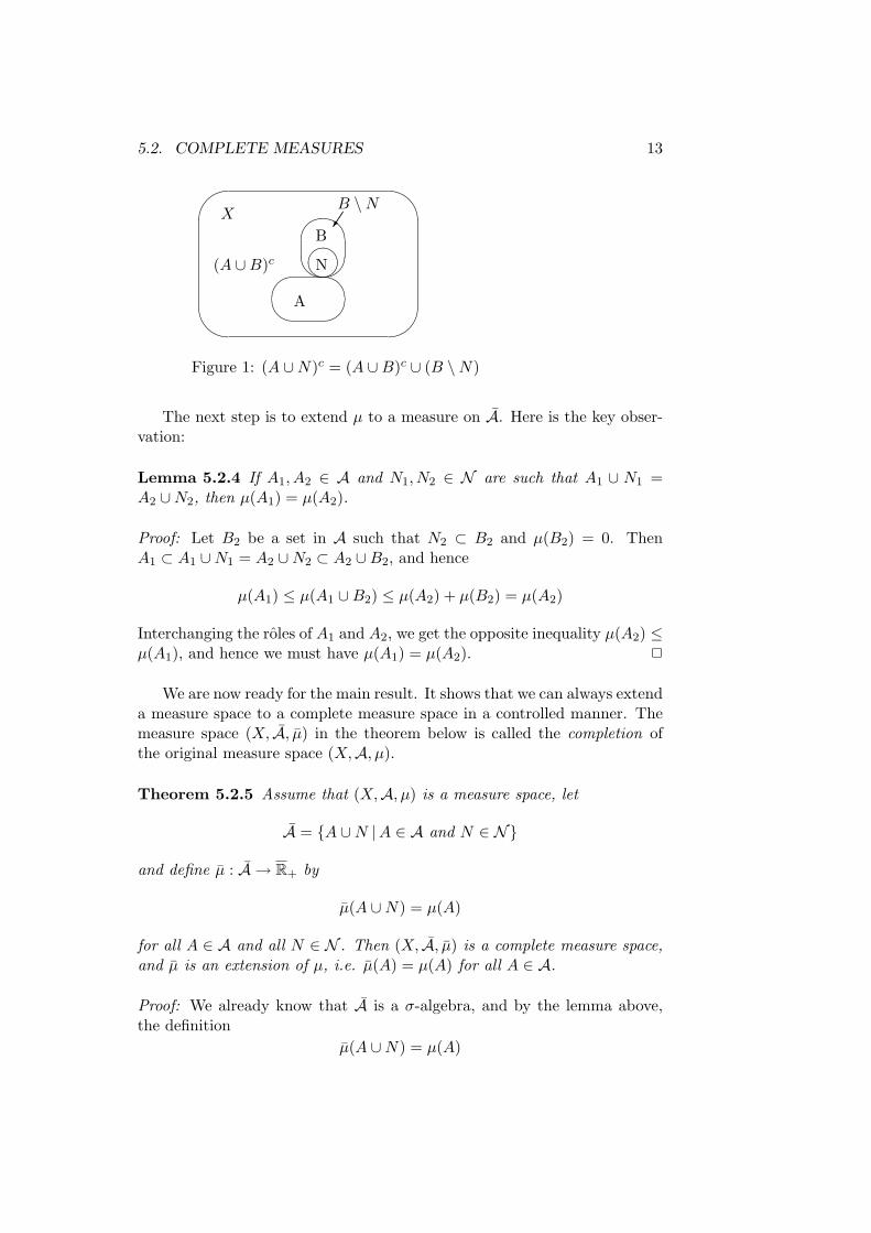
set A∪N ∈ A, we must prove that (A∪N)c ∈ A. Observe first that we canassume that A and N are disjoint; if not, we just replace N by N \A. Nextobserve that since N is a null set, there is a set B ∈ A such that N ⊂ Band µ(B) = 0. We may also assume that A and B are disjoint; if not, wejust replace B by B \A. Since

(A ∪N)c = (A ∪B)c ∪ (B \N)

(see Figure 1), where (A∪B)c ∈ A and B\N ∈ N , we see that (A∪N)c ∈ Aand the lemma is proved. 2


'

&

$

%

A

N

BX

(A ∪B)c

B \N

Figure 1: (A ∪N)c = (A ∪B)c ∪ (B \N)

The next step is to extend µ to a measure on A. Here is the key obser-vation:

Lemma 5.2.4 If A1, A2 ∈ A and N1, N2 ∈ N are such that A1 ∪ N1 =A2 ∪N2, then µ(A1) = µ(A2).

Proof: Let B2 be a set in A such that N2 ⊂ B2 and µ(B2) = 0. ThenA1 ⊂ A1 ∪N1 = A2 ∪N2 ⊂ A2 ∪B2, and hence

µ(A1) ≤ µ(A1 ∪B2) ≤ µ(A2) + µ(B2) = µ(A2)

Interchanging the roles of A1 and A2, we get the opposite inequality µ(A2) ≤µ(A1), and hence we must have µ(A1) = µ(A2). 2

We are now ready for the main result. It shows that we can always extenda measure space to a complete measure space in a controlled manner. Themeasure space (X, A, µ) in the theorem below is called the completion ofthe original measure space (X,A, µ).

Theorem 5.2.5 Assume that (X,A, µ) is a measure space, let

A = A ∪N |A ∈ A and N ∈ N

and define µ : A → R+ by

µ(A ∪N) = µ(A)

for all A ∈ A and all N ∈ N . Then (X, A, µ) is a complete measure space,and µ is an extension of µ, i.e. µ(A) = µ(A) for all A ∈ A.

Proof: We already know that A is a σ-algebra, and by the lemma above,the definition

µ(A ∪N) = µ(A)


is legitimate (i.e. it only depends on the set A ∪ N and not on the setsA ∈ A, N ∈ N we use to represent it). Also, we clearly have µ(A) = µ(A)for all A ∈ A.

To prove that µ is a measure, observe that since obviously µ(∅) = 0, wejust need to check that if Bn is a disjoint sequence of sets in A, then

µ(⋃n∈N

Bn) =∞∑

n=1

µ(Bn)

For each n, pick sets An ∈ A, Nn ∈ N such that Bn = An ∪Nn. Then theAn’s are clearly disjoint since the Bn’s are, and since

⋃n∈N Bn =

⋃n∈N An∪⋃

n∈N Nn, we get

µ(⋃n∈N

Bn) = µ(⋃n∈N

An) =∞∑

n=1

µ(An) =∞∑

n=1

µ(Bn)

It remains to check that µ is complete. Assume that C ⊂ D, whereµ(D) = 0; we must show that C ∈ A. Since µ(D) = 0, D is of the formD = A∪N , where A is in A with µ(A) = 0, and N is in N . By definition ofN , there is a B ∈ A such that N ⊂ B and µ(B) = 0. But then C ⊂ A ∪B,where µ(A ∪B) = 0, and hence C is in N and hence in A. 2

In Lemma 5.2.3 we proved that A is the smallest σ-algebra containing Aand N . This an instance of a more general phenomenon: Given a collectionB of subsets of X, there is always a smallest σ-algebra A containing B. Itis called the σ-algebra generated by B and is often designated by σ(B). Theproof that σ(B) exists is not difficult, but quite abstract:

Proposition 5.2.6 Let X be a non-empty set and B a collection of subsetsof X. Then there exists a smallest σ-algebra σ(B) containing B (in the sensethat if C is any other σ-algebra containing B, then σ(B) ⊂ C).

Proof: Observe that there is at least one σ-algebra containing B, namely theσ-algebra of all subsets of X. This guarantees that the following definitionmakes sense:

σ(B) = A ⊂ X |A belongs to all σ-algebras containing B

It suffices to show that σ(B) is a σ-algebra as it then clearly must be thesmallest σ-algebra containing B.

We must check the three conditions in Definition 5.1.1. For (i), justobserve that since ∅ belongs to all σ-algebras, it belongs to σ(B). For (ii),observe that if A ∈ σ(B), then A belongs to all σ-algebras containing B.Since σ-algebras are closed under complements, Ac belongs to the same σ-algebras, and hence to σ(B). The argument for (iii) is similar: Assume that


the sets An, n ∈ N, belong to σ(B). Then they belong to all σ-algebrascontaining B, and since σ-algebras are closed under countable unions, theunion

⋃n∈N An belongs to the same σ-algebras and hence to σ(B). 2

In many applications, the underlying set X is also a metric space (e.g.,X = Rd for the Lebesgue measure). In this case the σ-algebra σ(G) gener-ated by the collection G of open sets is called the Borel σ-algebra, a measuredefined on σ(G) is called a Borel measure, and the sets in σ(G) are calledBorel sets. Most useful measures on metric spaces are either Borel measuresor completions of Borel measures.

We can now use the results and terminology of this section to give amore detailed descriptions of the Lebesgue measure on Rd. It turns out (aswe shall prove in the next chapter) that there is a unique measure on theBorel σ-algebra σ(G) such that

µ([a1, b1]× [a2, b2]× · · · × [ad, bd]) = (b1 − a1)(b2 − a2) · . . . · (bd − ad)

whenever a1 < b1, a2 < b2,. . . , ad < bd (i.e. µ assigns the “right” valueto all rectangular boxes). The completion of this measure is the Lebesguemeasure on Rd.

We can give a similar description of the space of all infinite series of cointosses in Example 8 of section 5.1. In this setting one can prove that thereis a unique measure on the σ-algebra σ(C) generated by the cylinder sets,and the completion of this measure is the one used to model coin tossing.

Exercises to Section 5.2

1. Let X = 0, 1, 2 and let A = ∅, 0, 1, 2, X.

a) Show that A is a σ-algebra.

b) Define µ : A → R+ by: µ(∅) = µ(0, 1) = 0, µ(2) = µ(X) = 1.Show that µ is a measure.

c) Show that µ is not complete, and describe the completion (X, A, µ) of(X,A, µ).

2. Redo Problem 1 for X = 0, 1, 2, 3 and A = ∅, 0, 1, 2, 3, X.

3. Let (X,A, µ) be a complete measure space. Assume that A,B ∈ A withµ(A) = µ(B) < ∞. Show that if A ⊂ C ⊂ B, then C ∈ A.

4. Let A and B be two collections of subsets of X. Assume that any set in Abelongs to σ(B) and that any set in B belongs to σ(A). Show that σ(A) =σ(B).

5. Assume that X is a metric space, and let G be the collection of all open setsand F the collection of all closed sets. Show that σ(G) = σ(F).


6. Let X be a set. An algebra is a collection A of subset of X such that

(i) ∅ ∈ A(ii) If A ∈ A, then Ac ∈ A.

(iii) If A,B ∈ A, then A ∪B ∈ A.

Show that if B is a collection of subsets of X, there is a smallest algebra Acontaining B.

7. Let X be a set. A monotone class is a collection M of subset of X such that

(i) If An is an increasing sequence of sets from M, then⋃

n∈N An ∈M.

(ii) If An is a decreasing sequence of sets from M, then⋂

n∈N An ∈M.

Show that if B is a collection of subsets of X, there is a smallest monotoneclass M containing B.

5.3 Measurable functions

One of the main purposes of measure theory is to provide a richer and moreflexible foundation for integration theory, but before we turn to integration,we need to look at the functions we hope to integrate, the measurable func-tions. As functions taking the values ∞ and −∞ will occur naturally aslimits of sequences of ordinary functions, we choose to include them fromthe beginning; hence we shall study functions

f : X → R

where (X,A, µ) is a measure space and R = R ∪ −∞,∞ is the set ofextended real numbers. Don’t spend too much effort on trying to figureout what −∞ and ∞ “really” are — they are just convenient symbols fordescribing divergence.

To some extent we may extend ordinary algebra to R, e.g., we shall let

∞+∞ = ∞, −∞−∞ = −∞

and∞ ·∞ = ∞, (−∞) · ∞ = −∞, (−∞) · (−∞) = ∞.

If r ∈ R, we similarly let

∞+ r = ∞, −∞+ r = −∞

For products, we have to take the sign of r into account, hence

∞ · r =

∞ if r > 0

−∞ if r < 0

5.3. MEASURABLE FUNCTIONS 17

and similarly for (−∞) · r.All the rules above are natural and intuitive. Expressions that do not

have an intuitive interpretation, are usually left undefined, e.g. is ∞−∞not defined. There is one exception to this rule; it turns out that in measuretheory (but not in other parts of mathematics!) it is convenient to define0 · ∞ = ∞ · 0 = 0.

Since algebraic expressions with extended real numbers are not alwaysdefined, we need to be careful and always check that our expressions makesense.

We are now ready to define measurable functions:

Definition 5.3.1 Let (X,A, µ) be a measure space. A function f : X → Ris measurable (with respect to A) if

f−1([−∞, r)) ∈ A

for all r ∈ R. In other words, the set

x ∈ X : f(x) < r

must be measurable for all r ∈ R.

The half-open intervals in the definition are just a convenient startingpoint for showing that the inverse images of open and closed sets are mea-surable, but to prove this, we need a little lemma:

Lemma 5.3.2 Any non-empty, open set G in R is a countable union ofopen intervals.

Proof: Call an open interval (a, b) rational if the endpoints a, b are rationalnumbers. As there are only countably many rational numbers, there areonly countably many rational intervals. It is not hard to check that G is theunion of those rational intervals that are contained in G. 2

Proposition 5.3.3 If f : X → R is measurable, then f−1(I) ∈ A for allintervals I = (s, r), I = (s, r], I = [s, r), I = [s, r] where s, r ∈ R. Indeed,f−1(A) ∈ A for all open and closed sets A.

Proof: We use that inverse images commute with intersections, unions andcomplements. First observe that for any r ∈ R

f−1([−∞, r]

)= f−1

( ⋂n∈N

[−∞, r +1n

))

=⋂n∈N

f−1([−∞, r +

1n

))∈ A


which shows that the inverse images of closed intervals [−∞, r] are measur-able. Taking complements, we see that the inverse images of intervals of theform [s,∞] and (s,∞] are measurable:

f−1([s,∞]) = f−1([−∞, s)c) =(f−1([−∞, s)

))c ∈ A

andf−1((s,∞]) = f−1([−∞, s]c) =

(f−1([−∞, s]

))c ∈ A

To show that the inverse images of finite intervals are measurable, we justtake intersections, e.g.,

f−1((s, r)) = f−1([−∞, r) ∩ (s,∞]) = f−1([−∞, r)) ∩ f−1((s,∞]) ∈ A

If A is open, we know from the lemma above that it is a countable unionA =

⋃n∈N In of open intervals. Hence

f−1(A) = f−1( ⋃

n∈NIn

)=⋃n∈N

f−1(In) ∈ A

Finally, if A is closed, we use that its complement is open to get

f−1(A) =(f−1(Ac)

)c ∈ A2

It is sometimes convenient to use other kinds of intervals than those inthe definition to check that a function is measurable:

Proposition 5.3.4 Let (X,A, µ) be a measure space and consider a func-tion f : X → R. If either

(i) f−1([−∞, r]) ∈ A for all r ∈ R, or

(ii) f−1([r,∞]) ∈ A for all r ∈ R, or

(iii) f−1((r,∞]) ∈ A for all r ∈ R,

then f is measurable.

Proof: In either case we just have to check that f−1([−∞, r)) ∈ A for allr ∈ R. This can be done by the techniques in the previous proof. The detailsare left to the reader. 2

The next result tells us that there are many measurable functions. Recallthe definition of Borel measures and completed Borel measures from the endof Section 5.2.


Proposition 5.3.5 Let (X, d) be a metric space and let µ be a Borel or acompleted Borel measure on X. Then all continuous functions f : X → Rare measurable.

Proof: Since f is continuous and takes values in R,

f−1([−∞, r)) = f−1((−∞, r))

is an open set by Proposition 2.3.9 and measurable since the Borel σ-algebrais generated by the open sets. 2

We shall now prove a series of results showing how we can obtain newmeasurable functions from old ones. These results are not very exciting, butthey are necessary for the rest of the theory. Note that the functions in thenext two propositions take values in R and not R.

Proposition 5.3.6 Let (X,A, µ) be a measure space. If f : X → R ismeasurable, then φf is measurable for all continuous functions φ : R → R.In particular, f2 is measurable.

Proof: We have to check that

(φ f)−1((−∞, r)) = f−1(φ−1((−∞, r)))

is measurable. Since φ is contiunuous, φ−1((−∞, r)) is open, and con-sequently f−1(φ−1((−∞, r))) is measurable by Proposition 5.3.3. To seethat f2 is measurable, apply the first part of the theorem to the functionφ(x) = x2. 2

Proposition 5.3.7 Let (X,A, µ) be a measure space. If the functions f, g :X → R are measurable, so are f + g, f − g, and fg.

Proof: To prove that f +g is measurable, observe first that f +g < r meansthat f < r − g. Since the rational numbers are dense, it follows that thereis a rational number q such that f < q < r − g. Hence

(f + g)−1([−∞, r)) = x ∈ X | (f + g) < r) =⋃q∈Q

(x ∈ X | f(x) < q ∩ x ∈ X | g < r − q)

which is measurable since Q is countable and a countabe union of measurablesets is measurable. A similar argument proves that f − g is measurable.

To prove that fg is measurable, note that by Proposition 5.3.6 and whatwe have already proved, f2, g2, and (f + g)2 are measurable, and hence

fg =12((f + g)2 − f2 − g2

)


is measurable (check the details). 2

We would often like to apply the result above to functions taking valuesin the extended real numbers, but the problem is that the expressions neednot make sense. As we shall mainly be interested in functions that are finiteexcept on a set of measure zero, there is a way out of the problem. Let usstart with the terminology.

Definition 5.3.8 Let (X,A, µ) be a measure space. We say that a mea-surable function f : X → R is finite almost everywhere if the set x ∈X : f(x) = ±∞ has measure zero. We say that two measurable functionsf, g : X → R are equal almost everywhere if the set x ∈ X : f(x) 6= g(x)has measure zero. We usually abbreviate “almost everywhere” by “a.e.”.

If the measurable functions f and g are finite a.e., we can modify themto get measurable functions f ′ and g′ which take values in R and are equala.e. to f and g, respectively (see exercise 13). By the proposition above,f ′ + g′, f ′ − g′ and f ′g′ are measurable, and for many purposes they aregood representatives for f + g, f − g and fg.

Let us finally see what happens to limits of sequences.

Proposition 5.3.9 Let (X,A, µ) be a measure space. If fn is a sequenceof measurable functions fn : X → R, then supn∈N fn(x), infn∈N fn(x),lim supn→∞ fn(x) and lim infn→∞ fn(x) are measurable. If the sequence con-verges pointwise, then limn→∞ fn(x) is a measurable function.

Proof: To see that f(x) = supn∈N fn(x) is measurable, we use Proposition5.3.4(iii). For any r ∈ R

f−1((r,∞)]) = x ∈ X : supn∈N

fn(x) > r =

=⋃n∈N

x ∈ X : fn(x) > r =⋃n∈N

f−1n ((r,∞]) ∈ A

and hence f is measurable by Propostion 5.3.4(iii). The argument forinfn∈N fn(x) is similar.

To show that lim supn→∞ fn(x) is measurable, first observe that thefunctions

gk(x) = supn≥k

fn(x)

are measurable by what we have already shown. Since

lim supn→∞

fn(x) = infk∈N

gk(x),

the measurability of lim supn→∞ fn(x) follows. A similar argument holds forlim infn→∞ fn(x). If the sequence converges pointwise, then limn→∞ fn(x) =


lim supn→∞ fn(x) and is hence measurable. 2

The results above are extremely important. Mathematical analysis aboundswith limit arguments, and knowing that the limit function is measurable, isoften a key ingredient in these arguments.


1. Show that if f : X → R is measurable, the sets f−1(∞) and f−1(−∞)are measurable.

2. Complete the proof of Proposition 5.3.3 by showing that f−1 of the intervals(−∞, r), (−∞, r], [r,∞), (r,∞), (−∞,∞), where r ∈ R, are measurable.

3. Prove Proposition 5.3.4.

4. Fill in the details in the proof of Lemma 5.3.2. Explain in particular whythere is only a countable number of rational intervals and why the open setG is the union of the rational intervals contained in it.

5. Show that if f1, f2, . . . , fn are measurable functions with values in R, thenf1 + f2 + · · ·+ fn and f1f2 · . . . · fn are measurable.

6. The indicator function of a set A ⊂ X is defined by

1A(x) =

1 if x ∈ A

0 otherwise

a) Show that 1A is a measurable function if and only if A ∈ A.

b) A simple function is a function f : X → R of the form

f(x) =n∑

i=1

ai1Ai(x)

where a1, a2, . . . , an ∈ R and A1, A2, . . . , An ∈ A. Show that all simplefunctions are measurable.

7. Show that if f is measurable, then f−1(B) ∈ A for all Borel sets B (it mayhelp to take a look at Exercise 5.1.8).

8. Let En be a disjoint sequence of measurable sets such that⋃∞

n=1 En = X,and let fn be a sequence of measurable functions. Show that the functiondefined by

f(x) = fn(x) when x ∈ En

is measurable.

9. Fill in the details of the proof of the fg part of Proposition 5.3.7. You maywant to prove first that if h : X → R is measurable, then so is h

2 .

10. Prove the inf- and the lim inf-part of Proposition 5.3.9.

11. Let us write f ∼ g to denote that f and g are two measurable functionswhich are equal a.e.. Show that ∼ is an equivalence relation, i.e.:


(i) f ∼ f

(ii) If f ∼ g, then g ∼ f .

(iii) If f ∼ g and g ∼ h, then f ∼ h.

12. Let (X,A, µ) be a measure space.

a) Assume that the measure space is complete. Show that if f : X → Ris measurable and g : X → R equals f almost everywhere, then g ismeasurable.

b) Show by example that the result in a) does not hold without the com-pleteness condition. You may, e.g., use the measure space in Exercise5.2.1.

13. Assume that the measurable function f : X → R is finite a.e. Define a newfunction f ′ : X → R by

f ′(x) =

f(x) if f(x) is finite

0 otherwise

Show that f ′ is measurable and equal to f a.e.

14. A sequence fn of measurable functions is said to converge almost every-where to f if there is a set A of measure 0 such that fn(x) → f(x) for allx /∈ A.

a) Show that if the measure space is complete, then f is necessarily mea-surable.

b) Show by example that the result in a) doesn’t hold without the com-pleteness assumption (take a look at Problem 12 above).

15. Let X be a set and F a collection of functions f : X → R. Show that there isa smallest σ-algebra A on X such that all the functions f ∈ F are measurablewith respect to A (this is called the σ-algebra generated by F). Show that ifX is a metric space and all the functions in F are continuous, then A ⊂ B,where B is the Borel σ-algebra.

5.4 Integration of simple functions

We are now ready to look at integration. The integrals we shall work withare of the form

∫f dµ where f is a measurable function and µ is a measure,

and the theory is at the same time a refinement and a generalization of theclassical theory Riemann integration that you know from calculus.

It is a refinement because if we choose µ to be the one-dimensionalLebesgue measure, the new integral

∫f dµ equals the traditional Riemann

integral∫

f(x) dx for all Riemann integrable functions, but is defined formany more functions. The same holds in higher dimensions: If µ is n-dimensional Lebesgue measure, then

∫f dµ equals the Riemann integral

5.4. INTEGRATION OF SIMPLE FUNCTIONS 23

∫f(x1, . . . , xn) dx1 . . . dxn for all Riemann integrable functions, but is de-

fined for many more functions. The theory is also a vast generalization ofthe old one as it will allow us to integrate functions on all measure spacesand not only on Rn.

One of the advantages of the new (Lebesgue) theory is that it will allowus to interchange limits and integrals:

limn→∞

∫fn dµ =

∫lim

n→∞fn dµ

in much greater generality than before. Such interchanges are of great im-portance in many arguments, but are problematic for the Riemann integralas there is in general no reason why the limit function limn→∞ fn should beRiemann integrable even when the individual functions fn are. Accordingto Proposition 5.3.9, limn→∞ fn is measurable whenever the fn’s are, andthis makes it much easier to establish limit theorems for the new kind ofintegrals.

We shall develop integration theory in three steps: In this section weshall look at integrals of so-called simple functions which are generaliza-tions of step functions; in the next section we shall introduce integrals ofnonnegative mesurable functions; and in section 5.6 we shall extend the the-ory to functions taking both positive and negative values.

Thoughout this section we shall be working with a measure space (X,A, µ).If A is a subset of X, we define its indicator function by

1A(x) =

1 if x ∈ A

0 otherwise

The indicator function is measurable if and only if A is measurable.A measurable function f : X → R is called a simple function if it takes

only finitely many different values a1, a2, . . . , an. We may then write

f(x) =n∑

i=1

a11Ai(x)

where the sets Ai = x ∈ X | f(x) = ai are disjoint and measurable. Notethat if one of the ai’s is zero, the term does not contribute to the sum, andit is occasionally convenient to drop it.

If we instead start with measurable sets B1, B2, . . . , Bm and real numbersb1, b2, . . . , bm, then

g(x) =m∑

i=1

bi1Bi(x)

is measurable and takes only finitely many values, and hence is a simplefunction. The difference between f and g is that the sets A1, A2, . . . , An in


f are disjoint with union X, and that the numbers a1, a2, . . . , an are distinct.The same need not be the case for g. We say that the simple function fis on standard form, while g is not (unless, of course, the bi’s happen to bedistinct and the sets Bi are disjoint and make up all of X).

You may think of a simple function as a generalized step function. Thedifference is that step functions are constant on intervals (in R), rectangles(in R2), or boxes (in higher dimensions), while a simple function need onlybe constant on much more complicated (but still measurable) sets.

We can now define the integral of a nonnegative simple function.

Definition 5.4.1 Assume that

f(x) =n∑

i=1

ai1Ai(x)

is a nonnegative simple function on standard form. Then the integral of fwith respect to µ is defined by∫

f dµ =n∑

i=1

aiµ(Ai)

Recall that we are using the convention that 0·∞ = 0, and hence aiµ(Ai) = 0if ai = 0 and µ(Ai) = ∞.

Note that the integral of an indicator function is∫1A dµ = µ(A)

To see that the definition is reasonable, assume that you are in R2. Sinceµ(Ai) measures the area of the set Ai, the product aiµ(Ai) measures in anintuitive way the volume of the solid with base Ai and height ai.

We need to know that the formula in the definition also holds when thesimple function is not on standard form. The first step is the following,simple lemma:

Lemma 5.4.2 If

g(x) =m∑

j=1

bj1Bj (x)

is a nonnegative simple function where the Bj’s are disjoint and X =⋃mj=1 Bj, then ∫

g dµ =n∑

j=1

bjµ(Bj)


Proof: The problem is that the values b1, b2, . . . , bm need not be distinct, butthis is easily fixed: If c1, c2, . . . , ck are the distinct values taken by g, let bi1 ,bi2 ,. . . ,bini

be the bj ’s that are equal to ci, and let Ci = Bi1 ∪Bi2 ∪ . . .∪Bini.

Then µ(Ci) = µ(Bi1) + µ(Bi2) + . . . + µ(Bini), and hence

m∑j=1

bjµ(Bj) =k∑

i=1

ciµ(Ci)

Since g(x) =∑k

i=1 ci1Ci(x) is the standard form representation of g, wehave ∫

g dµ =k∑

i=1

ciµ(Ci)

and the lemma is proved 2

The next step is also easy:

Proposition 5.4.3 Assume that f and g are two nonnegative simple func-tions, and let c be a nonnnegative, real number. Then

(i)∫

cf dµ = c∫

f dµ

(ii)∫

(f + g) dµ =∫

f dµ +∫

g dµ

Proof: (i) is left to the reader. To prove (ii), let

f(x) =n∑

i=1

ai1Ai(x)

g(x) =n∑

j=1

bj1Bj (x)

be standard form representations of f and g, and define Ci,j = Ai ∩Bj . Bythe lemma above ∫

f dµ =∑i,j

aiµ(Ci,j)

and ∫g dµ =

∑i,j

bjµ(Ci,j)

and also ∫(f + g) dµ =

∑i,j

(ai + bj)µ(Ci,j)

since the value of f + g on Ci,j is ai + bj 2


Remark: Using induction, we can extend part (ii) above to longer sums:∫(f1 + f2 + · · ·+ fn) dµ =

∫f1 dµ +

∫f2 dµ + . . . +

∫fn dµ

for all nonnegative, simple functions f1, f2, . . . , fn,

We can now prove that the formula in Definition 5.4.1 holds for all rep-resentations of simple functions, and not only the standard ones:

Corollary 5.4.4 If f(x) =∑

n=1 ai1Ai(x) is a step function with ai ≥ 0for all i, then ∫

f dµ =n∑

i=1

aiµ(Ai)

Proof: By the results above∫f dµ =

∫ n∑i=1

ai1Ai dµ =n∑

i=1

∫ai1Ai dµ =

n∑i=1

ai

∫1Ai dµ =

n∑i=1

aiµ(Ai)

2

We need to prove yet another almost obvious result. We write g ≤ f tosay that g(x) ≤ f(x) for all x.

Proposition 5.4.5 Assume that f and g are two nonnegative simple func-tions. If g ≤ f , then ∫

g dµ ≤∫

f dµ

Proof: We use the same trick as in the proof of Proposition 5.4.3: Let

f(x) =n∑

i=1

ai1Ai(x)

g(x) =m∑

j=1

bj1Bj (x)

be standard form representations of f and g, and define Ci,j = Ai ∩ Bj .Then ∫

f dµ =∑i,j

aiµ(Ci,j) ≥∑i,j

bjµ(Ci,j) =∫

g dµ

2

We shall end this section with a key result on limits of integrals, butfirst we need some notation. Observe that if f =

∑ni=1 ai1Ai is a simple


function and B is a measurable set, then 1Bf =∑n

i=1 ai1Ai∩B is also asimple function. We shall write∫

Bf dµ =

∫1Bf dµ

and call this the integral of f over B. The lemma below may seem obvious,but it is the key to many later results.

Lemma 5.4.6 Assume that B is a measurable set, b a positive real number,and fn an increasing sequence of nonnegative simple functions such thatlimn→∞ fn(x) ≥ b for all x ∈ B. Then limn→∞

∫B fn dµ ≥ bµ(B).

Proof: Let a be any positive number less than b, and define

An = x ∈ B | fn(x) ≥ a

Since fn(x) ↑ b for all x ∈ B, we see that the sequence An is increasingand that

B =∞⋃

n=1

An

By continuity of measure (Proposition 5.1.5(i)), µ(B) = limn→∞ µ(An), andhence for any positive number m less that µ(B), we can find an N ∈ N suchthat µ(An) > m when n ≥ N . Since fn ≥ a on An, we thus have∫

Bfn dµ ≥

∫An

a dµ = am

whenever n ≥ N . Since this holds for any number a less than b and anynumber m less than µ(B), we must have limn→∞

∫B fn dµ ≥ bµ(B). 2

To get the result we need, we extend the lemma to simple functions:

Proposition 5.4.7 Let g be a nonnegative simple function and assume thatfn is an increasing sequence of nonnegative simple functions such thatlimn→∞ fn(x) ≥ g(x) for all x. Then

limn→∞

∫fn dµ ≥

∫g dµ

Proof: Let g(x) =∑m

i=1 bi1B1(x) be the standard form of g. If any of thebi’s is zero, we may just drop that term in the sum, so that we from now onassume that all the bi’s are nonzero. By Corollary 5.4.3(ii), we have∫

B1∪B2∪...∪Bm

fn dµ =∫

(1B1 + 1B2 + . . . + 1Bm) fn dµ =


=∫

(1B1fn + 1B2fn + . . . + 1Bmfn) dµ =

=∫

B1

fn dµ +∫

B2

fn dµ + . . . +∫

Bm

fn dµ

By the lemma, limn→∞∫Bi

fn dµ ≥ biµ(Bi), and hence

limn→∞

∫fn dµ ≥ lim

n→∞

∫B1∪B2∪...∪Bm

fn dµ ≥m∑

i=1

biµ(Bi) =∫

g dµ

2

We are now ready to extend the integral to all positive, measurablefunctions. This will be the topic of the next section.


1. Show that if f is a measurable function, then the level set

Aa = x ∈ X | f(x) = a

is measurable for all a ∈ R.

2. Check that according to Definition 5.4.1,∫

1A dµ = µ(A) for all A ∈ A.

3. Prove part (i) of Proposition 5.4.3.

4. Show that if f1, f2, . . . , fn are simple functions, then so are

h(x) = maxf1(x), f2(x), . . . , fn(x)

andh(x) = minf1(x), f2(x), . . . , fn(x)

5. Let µ be Lebesgue measure, and define A = Q ∩ [0, 1]. The function 1A isnot integrable in the Riemann sense. What is

∫1A dµ?

6. Let f be a nonnegative, simple function on a measure space (X,A, µ). Showthat

ν(B) =∫

B

f dµ

defines a measure ν on (X,A).

5.5 Integrals of nonnegative functions

We are now ready to define the integral of a general, nonnegative, measurablefunction. Throughout the sextion, (X,A, µ) is a measure space.

Definition 5.5.1 If f : X → R+ is measurable, we define∫f dµ = sup

∫g dµ | g is a nonnegative simple function, g ≤ f

5.5. INTEGRALS OF NONNEGATIVE FUNCTIONS 29

Remark: Note that if f is a simple function, we now have two definitionsof∫

f dµ; the original one in Definition 5.4.1 and a new one in the definitionabove. It follows from Proposition 5.4.5 that the two definitions agree.

The definition above is natural, but also quite abstract, and we shall worktoward a reformulation that is often easier to handle.

Proposition 5.5.2 Let f : X → R+ be a measurable function, and assumethat hn is an increasing sequence of simple functions converging pointwiseto f . Then

limn→∞

∫hn dµ =

∫f dµ

Proof: Since the sequence ∫

hn dµ is increasing by Proposition 5.4.5, thelimit clearly exists (it may be ∞), and since

∫hn dµ ≤

∫f dµ for all n, we

must havelim

n→∞

∫hn dµ ≤

∫f dµ

To get the opposite inequality, it suffices to show that

limn→∞

∫hn dµ ≥

∫g dµ

for each simple function g ≤ f , but this follows from Proposition 5.4.7. 2

The proposition above would lose much of its power if there weren’t anyincreasing sequences of simple functions converging to f . The next resulttells us that there always are. Pay attention to the argument; it is a key towhy the theory works.

Proposition 5.5.3 If f : X → R+ is measurable, there is an increasingsequence hn of simple functions converging pointwise to f . Moreover, foreach n either f(x)− 1

2n < hn(x) ≤ f(x) or hn(x) = 2n

Proof: To construct the simple function hn, we cut the interval [0, 2n) intohalf-open subintervals of length 1

2n , i.e. intervals

Ik =[

k

2n,k + 12n

)where 0 ≤ k < 22n, and then let

Ak = f−1(Ik)

We now define

hn(x) =22n−1∑k=0

k

2n1Ak

(x) + 2n1x | f(x)≥2n


By definition, hn is a simple function no greater than f . Since the intervalsget narrower and narrower and cover more and more of [0,∞), it is easy tosee that hn converges pointwise to f . To see why the sequence increases,note that each time we increase n by one, we split each of the former intervalsIk in two, and this will cause the new step function to equal the old one forsome x’s and jump one step upwards for others (make a drawing).

The last statement follows directly from the construction. 2

Remark: You should compare the partitions in the proof above to the par-titions you have earlier seen in Riemann integration. When we integratea function of one variable in calculus, we partition an interval [a, b] on thex-axis and use this partition to approximate the original function by a stepfunction. In the proof above, we instead partitioned the y-axis into inter-vals and used this partition to approximate the original function by a simplefunction. The latter approach gives us much better control over what is go-ing one; the partition controls the oscillations of the function. The price wehave to pay, it that we get simple functions instead of step functions, andto use simple functions for integration, we need measure theory.

Let us combine the last two results in a handy corollary:

Corollary 5.5.4 If f : X → R+ is measurable, there is an increasing se-quence hn of simple functions converging pointwise to f , and∫

f dµ = limn→∞

∫hn dµ

Let us take a look at some properties of the integral.

Proposition 5.5.5 Assume that f, g : X → R+ are measurable functionsand that c is a nonnegative, real number. Then:

(i)∫

cf dµ = c∫

f dµ.

(ii)∫

(f + g) dµ =∫

f dµ +∫

g dµ.

(iii) If g ≤ f , then∫

g dµ ≤∫

f dµ.

Proof: (iii) is immediate from the definition, and (i) is left to the reader. Toprove (ii), let fn and gn be to increasing sequence of simple functionsconverging to f and g, respectively. Then fn+gn is an increasing sequenceof simple functions converging to f + g, and∫

(f + g) dµ = limn→∞

∫(fn + gn) dµ = lim

n→∞

(∫fn dµ +

∫gn dµ

)=

= limn→∞

∫fn dµ + lim

n→∞

∫gn dµ =

∫f dµ +

∫g dµ


where we have used Proposition 5.4.3(ii) to go from∫

(fn+gn) dµ to∫

fn dµ+∫gn dµ. 2

One of the great advantages of the Lebesgue integration theory we arenow developing is that it is much better behaved with respect to limits thanthe Riemann theory you are used to. Here is a typical example:

Theorem 5.5.6 (Monotone Convergence Theorem) If fn is an in-creasing sequence of nonnegative, measurable functions such that f(x) =limn→∞ fn(x) for all x, then

limn→∞

∫fn dµ =

∫f dµ

In other words,

limn→∞

∫fn dµ =

∫lim

n→∞fn dµ

Proof: We know from Proposition 5.3.8 that f is measurable, and hence theintegral

∫f dµ is defined. Since fn ≤ f , we have

∫fn dµ ≤

∫f dµ for all n,

and hence

limn→∞

∫fn dµ ≤

∫f dµ

To prove the opposite inequality, we approximate each fn by simple functionsas in the proof of Proposition 5.5.3; in fact, let hn be the n-th approximationto fn. Assume that we can prove that the sequence hn converges to f ;then

limn→∞

∫hn dµ =

∫f dµ

by Proposition 5.5.2. Since fn ≥ hn, this would give us the desired inequality

limn→∞

∫fn dµ ≥

∫f dµ

It remains to show that hn(x) → f(x) for all x. From Proposition 5.5.3we know that for all n, either fn(x)− 1

2n < hn(x) ≤ fn(x) or hn(x) = 2n. Ifhn(x) = 2n for infinitely many n, then hn(x) goes to ∞, and hence to f(x).If hn(x) is not equal to 2n for infinitely many n, then we eventually havefn(x)− 1

2n < hn(x) ≤ fn(x), and hence hn(x) converges to f(x) since fn(x)does. 2

We would really have liked the formula

limn→∞

∫fn dµ =

∫lim

n→∞fn dµ (5.5.1)


above to hold in general, but as the following example shows, this is not thecase.

Example 1: Let µ be the counting measure on N, and define the sequencefn by

fn(x) =

1 if x = n

0 otherwise

Then limn→∞ fn(x) = 0 for all x, but∫

fn dµ = 1. Hence

limn→∞

∫fn dµ = 1

but ∫lim

n→∞fn dµ = 0

♣

There are many results in measure theory giving conditions for (5.5.1) tohold, but there is no ultimate theorem covering all others. There is, however,a simple inequality that always holds.

Theorem 5.5.7 (Fatou’s Lemma) Assume that fn is a sequence of non-negative, measurable functions. Then

lim infn→∞

∫fn dµ ≥

∫lim infn→∞

fn dµ

Proof: Let gk(x) = infk≥n fn(x). Then gk is an increasing sequence ofmeasurable functions, and by the Monotone Convergence Theorem

limk→∞

∫gk dµ =

∫lim

k→∞gk dµ =

∫lim infn→∞

fn dµ

where we have used the definition of lim inf in the last step. Since fk ≥ gk,we have

∫fk dµ ≥

∫gk dµ, and hence

lim infk→∞

∫fk dµ ≥ lim

k→∞

∫gk dµ =

∫lim infn→∞

fn dµ

and the result is proved. 2

Fatou’s Lemma is often a useful tool in establishing more sophisticatedresults, see Exercise 16 for a typical example.

Just as for simple functions, we define integrals over measurable subsetsA of X by the formula


∫A

f dµ =∫

1Af dµ

So far we have allowed our integrals to be infinite, but we are mainlyinterested in situations where

∫f dµ is finite:

Definition 5.5.8 A function f : X → [0,∞] is said to be integrable if it ismeasurable and

∫f dµ < ∞.

Comparison with Riemann integration

We shall end this section with a quick comparison between the integral wehave now developed and the Riemann integral you learned in calculus. Letus begin with a quick review of the Riemann integral1.

Assume that [a, b] is a closed and bounded interval, and let f : [a, b] → Rbe a nonnegative, bounded function. Recall that a partition P of the interval[a, b] is a finite set x0, x1, . . . , xn such that

a = x0 < x1 < x2 < . . . < xn = b

The lower and upper values of f over the interval (xi−1, xi] are

mi = inff(x) |x ∈ (xi−1, xi]

andMi = supf(x) |x ∈ (xi−1, xi]

respectively, and the lower and upper sums of the partition P are

L(P) =n∑

i=1

mi(xi − xi−1)

and

U(P) =n∑

i=1

Mi(xi − xi−1)

The function f is Riemann integrable if the lower integral∫ b

af(x) dx = supL(P) | P is a partition of [a, b]

and the upper integral∫ b

af(x) dx = infU(P) | P is a partition of [a, b]

1The approach to Riemann integration that I describe here is actually due to the Frenchmathematician Gaston Darboux (1842-1917).


coincide, in which case we define the Riemann integral∫ ba f(x) dx to be the

common value.We are now ready to compare the Riemann integral

∫ ba f(x) dx and the

Lebesgue integral∫[a,b] f dµ (µ is now the Lebesgue measure). Observe first

that if we define simple functions

φP =n∑

i=1

mi1(xi−1,xi]

and

ΦP =n∑

i=1

Mi1(xi−1,xi]

we have ∫φP dµ =

n∑i=1

mi(xi − xi−1) = N(P)

and ∫ΦP dµ =

n∑i=1

Mi(xi − xi−1) = U(P)

Theorem 5.5.9 Assume that f : [a, b] → [0,∞) is a bounded, Riemannintegrable function on [a, b]. Then f is measurable and the Riemann and theLebesgue integral coincide:∫ b

af(x) dx =

∫[a.b]

f dµ

Proof: Since f is Riemann integrable, we can pick a sequence Pn of parti-tions such that the sequences φ(Pn) of lower step functions is increasing,the sequence Φ(Pn) of upper step functions is decreasing, and

limn→∞

L(Pn) = limn→∞

U(Pn) =∫ b

af(x) dx

(see Exercise 10 for help), or in other words

limn→∞

∫φPn dµ = lim

n→∞

∫ΦPn dµ =

∫ b

af(x) dx

This means thatlim

n→∞

∫(ΦPn − φPn) dµ = 0

and by Fatou’s lemma, we have∫lim

n→∞(ΦPn − φPn) dµ = 0


(the limits exists since the sequence ΦPn − φPn is decreasing). This meansthat limn→∞ φPn = limn→∞ ΦPn a.e., and since

limn→∞

φPn ≤ f ≤ limn→∞

ΦPn ,

f must be measurable as it squeezed between two almost equal, measurablefunctions. Also, since f = limn→∞ φPn a.s., the Monotone ConvergenceTheorem (we are actually using the slightly extended version in Exercise13) tells us that∫

[a,b]f dµ = lim

n→∞

∫φPn dµ = lim

n→∞U(Pn) =

∫ b

af(x) dx

2

The theorem above can be extended in many directions. Exactly the sameproof works for Riemann integrals over rectangular boxes in Rd, and oncewe have introduced integrals of functions taking both positive and negativevalues in the next section, it easy to extend the theorem above to thatsituation. There are some subtleties concerning improper integrals, but weshall not touch on these here. Our basic message is: Lebesgue integrationis just like Riemann integration, only better (because more functions areintegrable and we can integrate in completely new contexts — all we needis a measure)!


1. Assume f : X → [0,∞] is a nonnegative simple function. Show that the twodefinitions of

∫f dµ given in Definitions 5.4.1 and 5.5.1 coincide.

2. Prove Proposition 5.5.5(i).

3. Show that if f : X → [0,∞] is measurable, then

µ(x ∈ X | f(x) ≥ a) ≤ 1a

∫f dµ

for all positive, real numbers a.

4. In this problem, f, g : X → [0,∞] are measurable functions.

a) Show that∫

f dµ = 0 if and only if f = 0 a.e.

b) Show that if f = g a.e., then∫

f dµ =∫

g dµ.

c) Show that if∫

Ef dµ =

∫E

g dµ for all measurable sets E, then f = ga.e.

5. Assume that (X,A, µ) is a measure space and that f : X → [0,∞] is anonnegative, measurable function

a) Show that if A, B are measurable sets with A ⊂ B, then∫

Af dµ ≤∫

Bf dµ


b) Show that if A,B are disjoint, measurable sets, then∫

A∪Bf dµ =∫

Af dµ +

∫B

f dµ.

c) Define ν : A → R by

ν(A) =∫

A

f dµ

Show that ν is a measure.

6. Show that if f : X → [0,∞] is integrable, then f is finite a.e.

7. Let µ be Lebesgue measure on R and assume that f : R → R+ is a nonneg-ative, measurable function. Show that

limn→∞

∫[−n,n]

f dµ =∫

f dµ

8. Let µ be Lebesgue measure on R. Show that for all measurable sets A ⊂ R

limn→∞

∫A

n∑k=1

x2k

k!dµ =

∫A

ex2dµ

9. Let f : R → R be the function

f(x) =

1 if x is rational

0 otherwise

and for each n ∈ N, let fn : R → R be the function

fn(x) =

1 if x = p

q where p ∈ Z, q ∈ N, q ≤ n

0 otherwise

a) Show that fn(x) is an increasing sequence converging to f(x) for allx ∈ R.

b) Show that each fn is Riemann integrable over [0, 1] with∫ 1

0fn(x) dx = 0

(this is integration as taught in calculus courses).c) Show that f is not Riemann integrable over [0, 1].d) Show that the one-dimensional Lebesgue integral

∫[0,1]

f dµ exists andfind its value.

10. In this problem we shall sketch how one may construct the sequence Pn ofpartitions in the proof of Theorem 5.5.9.

a) Call a partition P of [a, b] finer than another partition Q if Q ⊂ P, andshow that if P is finer than Q, then φP ≥ φQ and ΦP ≤ ΦQ.

b) Show that if f is as in Theorem 5.5.9, there are sequences of partitionsQn and Rn such that

limn→∞

L(Qn) =∫ b

a

f(x) dx

and

limn→∞

U(Rn) =∫ b

a

f(x) dx


c) For each n, let Pn be the common refinement of all partitions Qk andRk, k ≤ n, i.e.

Pn =n⋃

k=1

(Qk ∪Rk)

Show that Pn satisfies the requirements in the proof of Theorem 5.5.9.

11. a) Let un be a sequence of positive, measurable functions. Show that∫ ∞∑n=1

un dµ =∞∑

n=1

∫un dµ

b) Assume that f is a nonnnegative, measurable function and that Bnis a disjoint sequence of measurable sets with union B. Show that∫

B

f dµ =∞∑

n=1

∫Bn

f dµ

12. Assume that f is a nonnegative, measurable function and that An is anincreasing sequence of measurable sets with union A. Show that∫

A

f dµ = limn→∞

∫An

f dµ

13. Show the following generalization of the Monotone Convergence Theorem:If fn is an increasing sequence of nonnegative, measurable functions suchthat f(x) = limn→∞ fn(x) almost everywhere. (i.e. for all x outside a set Nof measure zero), then

limn→∞

∫fn dµ =

∫f dµ

14. Find a decreasing sequence fn of measurable functions fn : R → [0,∞)converging pointwise to zero such that limn→∞

∫fn dµ 6= 0

15. Assume that f : X → [0,∞] is a measurable function, and that fn is asequence of measurable functions converging pointwise to f . Show that iffn ≤ f for all n,

limn→∞

∫fn dµ =

∫f dµ

16. Assume that fn is a sequence of nonnegative functions converging pointwiseto f . Show that if

limn→∞

∫fn dµ =

∫f dµ < ∞,

then

limn→∞

∫E

fn dµ =∫

E

f dµ

for all measurable E ⊂ X.


17. Assume that g : X → [0,∞] is an integrable function, and that fn isa sequence of nonnegative, measurable functions converging pointwise to afunction f . Show that if fn ≤ g for all n, then

limn→∞

∫fn dµ =

∫f dµ

Hint: Apply Fatou’s Lemma to both sequences fn and g − fn.

18. Let (X,A) be a measurable space, and let M+ be the set of all non-negative,measurable functions f : X → R+. Assume that I : M+ → R+ satisfies thefollowing three conditions:

(i) I(αf) = αI(f) for all α ∈ [0,∞) and all f ∈M+.(ii) I(f + g) = I(f) + I(g) for all f, g ∈M+.(iii) If fn is an increasing sequence from M+ converging pointwise to f ,

then limn→∞ I(fn) = I(f).

a) Show that I(f1 + f2 + · · · + fn) = I(f1) + I(f2) + · · · + I(fn) for alln ∈ N and all f1, f2, . . . , fn ∈M+.

b) Show that if f, g ∈M+ and f(x) ≤ g(x) for all x ∈ X, then I(f) ≤ I(g).c) Show that

µ(E) = I(1E) for E ∈ Adefines a measure on (X,A).

d) Show that I(f) =∫

f dµ for all non-negative simple functions f .e) Show that I(f) =

∫f dµ for all f ∈M+.

5.6 Integrable functions

So far we only know how to integrate nonnegative functions, but it is notdifficult to extend the theory to general functions. We have, however, tobe a little more careful with the size of the functions we integrate: If anonnegative function f is too big, we may just put the integral

∫f dµ equal

to ∞, but if the function can take negative values as well as positive, theremay be infinite contributions of opposite signs that are difficult to balance.For this reason we shall only define the integral for a class of integrablefunctions where this problem does not occur.

Given a function f : X → R, we first observe that f = f+ − f−, wheref+ and f− are the nonnegative functions

f+(x) =

f(x) if f(x) > 0

0 otherwise

and

f−(x) =

−f(x) if f(x) < 0

0 otherwise

5.6. INTEGRABLE FUNCTIONS 39

Note that f+ and f− are measurable if f is.Recall that a nonnegative, measurable function f is integrable if

∫f dµ <

∞.

Definition 5.6.1 A function f : X → R is called integrable if it is mea-surable, and f+ and f− are integrable. We define the integral of f by∫

f dµ =∫

f+ dµ−∫

f− dµ

The definition illustrates our point above: If both∫

f+ dµ and∫

f− dµ areinfinite, there is no natural way to define the difference

∫f+ dµ−

∫f− dµ.

The next lemma gives a useful characterization of integrable functions.

Lemma 5.6.2 A measurable function f is integrable if and only if its ab-solute value |f | is integrable, i.e. if and only if

∫|f | dµ < ∞.

Proof: Note that |f | = f+ + f−. Hence∫|f | dµ =

∫f+ dµ +

∫f− dµ

by Proposition 5.5.5(ii), and we see that∫|f | dµ is finite if and only if both∫

f+ dµ and∫

f− dµ are finite. 2

The next lemma is another useful technical tool. It tells us that if wesplit f as a difference f = g − h of two nonnegative, integrable functions,we always get

∫f dµ =

∫g dµ−

∫h dµ (so far we only know this for g = f+

and h = f−).

Lemma 5.6.3 Assume that g : X → [0,∞] and h : X → [0,∞] are twointegrable, nonnegative functions, and that f(x) = g(x)− h(x) at all pointswhere the difference is defined. Then f is integrable and∫

f dµ =∫

g dµ−∫

h dµ

Proof: Note that since g and h are integrable, they are finite a.e., and hencef = g − h a.e. Modifying g and h on a set of measure zero (this will notchange their integrals), we may assume that f(x) = g(x) − h(x) for all x.Since |f(x)| = |g(x) − h(x)| ≤ |g(x)| + |h(x)|, it follows from the lemmaabove that f is integrable.

Asf(x) = f+(x)− f−(x) = g(x)− h(x)

we havef+(x) + h(x) = g(x) + f−(x)


where we on both sides have sums of nonnegative functions. By Proposition5.5.5(ii), we get ∫

f+ dµ +∫

h dµ =∫

g dµ +∫

f− dµ

Rearranging the integrals (they are all finite), we get∫f dµ =

∫f+ dµ−

∫f− dµ =

∫g dµ−

∫h dµ

and the lemma is proved. 2

We are now ready to prove that the integral behaves the way we expect:

Proposition 5.6.4 Assume that f, g : X → R are integrable functions, andthat c is a constant. Then f + g and cf are integrable, and

(i)∫

cf dµ = c∫

f dµ.

(ii)∫

(f + g) dµ =∫

f dµ +∫

g dµ.

(iii) If g ≤ f , then∫

g dµ ≤∫

f dµ.

Proof: (i) is left to the reader (treat positive and negative c’s separately). Toprove (ii), first note that since f and g are integrable, the sum f(x) + g(x)is defined a.e., and by changing f and g on a set of measure zero (thisdoesn’t change their integrals), we may assume that f(x) + g(x) is definedeverywhere. Since

|f(x) + g(x)| ≤ |f(x)|+ |g(x)|,

f + g is integrable. Obviously,

f + g = (f+ − f−) + (g+ − g−) = (f+ + g+)− (f− + g−)

and hence by the lemma above and Proposition 5.5.5(ii)∫(f + g) dµ =

∫(f+ + g+) dµ−

∫(f− + g−) dµ =

=∫

f+ dµ +∫

g+ dµ−∫

f− dµ−∫

g− dµ =

=∫

f+ dµ−∫

f− dµ +∫

g+ dµ−∫

g− dµ =

=∫

f dµ +∫

g dµ


To prove (iii), note that f − g is a nonnegative function and hence by (i)and (ii):∫

f dµ−∫

g dµ =∫

f dµ +∫

(−1)g dµ =∫

(f − g) dµ ≥ 0

Consequently,∫

f dµ ≥∫

g dµ and the proposition is proved. 2

We can now extend our limit theorems to integrable functions takingboth signs. The following result is probably the most useful of all limittheorems for integrals as it is quite strong and at the same time easy touse. It tells us that if a convergent sequence of functions is dominated byan integrable function, then

limn→∞

∫fn dµ =

∫lim

n→∞fn dµ

Theorem 5.6.5 (Lebesgue’s Dominated Convergence Theorem) As-sume that g : X → R is a nonnegative, integrable function and that fn isa sequence of measurable functions converging pointwise to f . If |fn| ≤ gfor all n, then

limn→∞

∫fn dµ =

∫f dµ

Proof: First observe that since |f | ≤ g, f is integrable. Next note thatsince g − fn and g + fn are two sequences of nonnegative measurablefunctions, Fatou’s Lemma gives:

lim infn→∞

∫(g−fn) dµ ≥

∫lim infn→∞

(g−fn) dµ =∫

(g−f) dµ =∫

g dµ−∫

f dµ

and

lim infn→∞

∫(g+fn) dµ ≥

∫lim infn→∞

(g+fn) dµ =∫

(g+f) dµ =∫

g dµ+∫

f dµ

On the other hand,

lim infn→∞

∫(g − fn) dµ =

∫g dµ− lim sup

n→∞

∫fn dµ

andlim infn→∞

∫(g + fn) dµ =

∫g dµ + lim inf

n→∞

∫fn dµ

Combining the two expressions for lim infn→∞∫

(g − fn) dµ, we see that∫g dµ− lim sup

n→∞

∫fn dµ ≥

∫g dµ−

∫f dµ


and hence

lim supn→∞

∫fn dµ ≤

∫f dµ

Combining the two expressions for lim infn→∞∫

(g+fn) dµ, we similarly get

lim infn→∞

∫fn dµ ≥

∫f dµ

Hence

lim supn→∞

∫fn dµ ≤

∫f dµ ≤ lim inf

n→∞

∫fn dµ

which means that limn→∞∫

fn dµ =∫

f dµ. The theorem is proved. 2

Remark: It is easy to check that we can relax the conditions above some-what: If fn(x) converges to f(x) a.e., and |fn(x)| ≤ g(x) fails on a set ofmeasure zero, the conclusion still holds (see Exercise 7 for the precise state-ment).

Let us take a look at a typical application of the theorem:

Proposition 5.6.6 Let f : R×X → R be a function which is

(i) continuous in the first variable, i.e. for each y ∈ X, the functionx 7→ f(x, y) is continuous

(ii) measurable in the second component, i.e. for each x ∈ X, the functiony 7→ f(x, y) is measurable

(iii) uniformly bounded by an integrable function, i.e. there is an integrablefunction g : R → [0,∞] such that |f(x, y)| ≤ g(y) for all x, y ∈ R.

Then the function

h(x) =∫

f(x, y) dµ(y)

is continuous (the expression∫

f(x, y) dµ(y) means that we for each fixed xintegrate f(x, y) as a function of y).

Proof: According to Proposition 2.2.5 it suffices to prove that if an is asequence converging to a point a, then h(an) converges to h(a). Observethat

h(an) =∫

f(an, y) dµ(y)

and

h(a) =∫

f(a, y) dµ(y)


Observe also that since f is continuous in the first variable, f(an, y) →f(a, y) for all y. Hence f(an, y) is a sequence of functions which is domi-nated by the integrable function g and which converges pointwise to f(a, y).By Lebesgue’s Dominated Convergence Theorem,

limn→∞

h(an) = limn→∞

∫f(an, y) dµ =

∫f(a, y) dµ = h(a)

and the proposition is proved. 2

As before, we define∫A f dµ =

∫f1A dµ for measurable sets A. We say

that f is integrable over A if f1A is integrable.

Exercises to Section 5.6

1. Show that if f is measurable, so are f+ and f−.

2. Show that if an integrable function f is zero a.e., then∫

f dµ = 0.

3. Prove Proposition 5.6.4(i). You may want to treat positive and negative c’sseparately.

4. Assume that f : X → R is a measurable function.

a) Show that if f is integrable over a measurable set A, and An is anincreasing sequence of measurable sets with union A, then

limn→∞

∫An

f dµ =∫

A

f dµ

b) Assume that Bn is a decreasing sequence of measurable sets withintersection B. Show that if f is integrable over B1, then

limn→∞

∫Bn

f dµ =∫

B

f dµ

5. Show that if f : X → R is integrable over a measurable set A, and An is adisjoint sequence of measurable sets with union A, then∫

A

f dµ =∞∑

n=1

∫An

f dµ

6. Let f : R → R be a measurable function, and define

An = x ∈ X | f(x) ≥ n

Show that

limn→∞

∫An

f dµ = 0


7. Prove the following slight extension of the Dominated Convergence Theorem:

Theorem: Assume that g : X → R is a nonnegative, integrable functionand that fn is a sequence of measurable functions converging a.e. to f . If|fn(x)| ≤ g(x) a.e. for each n, then

limn→∞

∫fn dµ =

∫f dµ

8. Assume that g : R × X → R is continuous in the first variable and thaty → g(x, y) is integrable for each x. Assume also that the partial derivative∂g∂x (x, y) exists for all x and y, and that there is an integrable function h :R → [0,∞] such that ∣∣∣∣∂g

∂x(x, y)

∣∣∣∣ ≤ h(y)

for all x, y. Show that the function

f(x) =∫

g(x, y) dµ(y)

is differentiable at all points x and

f ′(x) =∫

∂g

∂x(x, y) dµ(y)

This is often referred to as “differentiation under the integral sign”.

9. Let µ be the Lebesgue measure on R. Show that if a, b ∈ R, a < b, andf : [a, b] → R is a bounded, Riemann integrable function, then f is integrableover [a, b] and ∫ b

a

f(x) dx =∫

[a,b]

f dµ

(Hint: Since f is bounded, there is a constant M such that f + M is non-negative. Apply Theorem 5.5.9 to this function.)

5.7 L1(X,A, µ) and L2(X,A, µ)

In this section we shall connect integration theory to the theory of normedspaces in Chapter 4. Recall from Definition 4.5.2 that a norm on a realvector space V is a function || · || : V → [0,∞) satisfying

(i) ||u|| ≥ 0 with equality if and only if u = 0.

(ii) ||αu|| = |α|||u|| for all α ∈ R and all u ∈ V .

(iii) ||u + v|| ≤ ||u||+ ||v|| for all u,v ∈ V .

5.7. L1(X,A, µ) AND L2(X,A, µ) 45

Let us now put

L1(X,A, µ) = f : X → R : f is integrable

and define || · ||1 : L1(X,A, µ) → [0,∞) by

||f ||1 =∫|f | dµ

It is not hard to see that L1(X) is a vector space (see Exercise 1), and that|| · ||1 satisfies the three axioms above with one exception; ||f ||1 may be zeroeven when f is not zero — actually ||f ||1 = 0 if and only if f = 0 a.e.

The usual way to fix this is to consider two functions f and g to be equalif they are equal almost everywhere. To be more precise, let us write f ∼ gif f and g are equal a.e., and define the equivalence class of f to be the set

[f ] = g ∈ L1(X,A, µ) | g ∼ f

Note that two such equivalence classes [f ] and [g] are either equal (if fequals g a.e.) or disjoint (if f is not equal to g a.e.). If we let L1(X,A, µ)be the collection of all equivalence classes, we can organize L1(X,A, µ) as anormed vector space by defining

α[f ] = [αf ] and [f ] + [g] = [f + g] and |[f ]|1 = ||f ||1

The advantage of the space (L1(X), | · |1) compared to (L1(X,A, µ), || · ||1)is that it is a normed space where all the theorems we have proved aboutsuch spaces apply — the disadvantage is that the elements are no longerfunctions, but equivalence classes of functions. In practice, there is very littledifference between (L1(X), |·|1) and (L1(X,A, µ), ||·||1), and mathematicianstend to blur the distinction between the two spaces: they pretend to work inL1(X,A, µ), but still consider the elements as functions. We shall follow thispractice here; it is totally harmless as long as you remember that wheneverwe talk about an element of L1(X,A, µ) as a function, we are really choosinga representative from an equivalence class (Exercise 3 gives a more thoroughand systematic treatment of L1(X,A, µ)).

The most important fact about (L1(X), | · |1) is that it is complete. Inmany ways, this is the most impressive success of the theory of measures andintegration: We have seen in previous chapters how important completenessis, and it is a great advantage to work with a theory of integration wherethe space of integrable functions is naturally complete. Before we turn tothe proof, you may want to remind yourself of Proposition 4.5.5 which shallbe our main tool.

Theorem 5.7.1 (L1(X), | · |1) is complete.


Proof: Assume that un is a sequence of functions in L1(X,A, µ) suchthat the series

∑∞n=1 un converges absolutely, i.e. that

∑∞n=1 |un|1 < ∞.

According to Proposition 4.5.5, it suffices to show that the series∑∞

n=1 un(x)must converge in L1(X,A, µ).

We first use the absolute convergence to prove that the series∑∞

n=1 |un(x)|converges to an integrable function:∫ ∞∑

n=1

|un| dµ =∫

limN→∞

N∑n=1

|un| dµ = limN→∞

∫ N∑n=1

|un| dµ

= limN→∞

N∑n=1

∫|un| dµ = lim

N→∞

N∑n=1

|un|1 =∞∑

n=1

|un|1 < ∞

where we have used the Monotone Convergence Theorem to move the limitinside the integral sign. This means that the function

g(x) =∞∑

n=1

|un(x)|

is integrable. We shall use g as the dominating function in the DominatedConvergence Theorem.

Let us first observe that since g(x) =∑∞

n=1 |un(x)| is integrable, theseries converges a.e. Hence the sequence

∑∞n=1 un(x) (without the absolute

values) converges absolutely a.e., and hence it converges a.e. in the ordinarysense. Let f(x) =

∑∞n=1 un(x) (put f(x) = 0 on the null set where the

series does not converge). It remains to prove that the series converges tof in L1-sense, i.e. that |f −

∑Nn=1 un|1 → 0 as N → ∞. By definition

of f , we know that limN→∞

(f(x)−

∑Nn=1 un(x)

)= 0 a.e. Since |f(x) −∑N

n=1 un(x)| = |∑∞

n=N+1 un(x)| ≤ g(x) a.e., it follows from DominatedConvergence Theorem (actually from the slight extension in Exercise 5.7.7)that

|f −N∑

n=1

un|1 =∫|f −

N∑n=1

un| dµ → 0

The theorem is proved. 2

It turns of that L1(X,A, µ) is just one of infinitely many spaces of thesame kind. In fact, for any real number p ≥ 1, we may let

Lp(X,A, µ) = f : X → R : |f |p is integrable

and define || · ||p : Lp(X,A, µ) → [0,∞) by

||f ||p =(∫

|f |p dµ

) 1p

5.7. L1(X,A, µ) AND L2(X,A, µ) 47

It turns out that Lp(X,A, µ) is a vector space, and that || · ||p is a norm onLp(X,A, µ), except that ||f ||p = 0 if f = 0 a.e. If we consider functions asequal if they are equal a.e., we can turn (Lp(X), || · ||p) into a normed space(Lp(X), | · |p) just as we did with L1(X,A, µ).

We shall not pursue the general theory of Lp-spaces here, but we shalltake a closer look at the case p = 2, i.e. the space

L2(X,A, µ) = f : X → R : |f |2 is integrable

with the norm

||f ||2 =(∫

|f |2 dµ

) 12

This space is particularly important as it turns out to be an inner productspace with inner product

〈f, g〉 =∫

fg dµ

But let us begin from the beginning. To prove that L2(X,A, µ) is a vectorspace, we need a simple lemma:

Lemma 5.7.2 For all real numbers a, b

(a + b)2 ≤ 2a2 + 2b2

Proof:2a2 + 2b2 − (a + b)2 = a2 + b2 − 2ab = (a− b)2 ≥ 0

2

It is now easy to prove that L2(X,A, µ) is a vector space:

Proposition 5.7.3 L2(X,A, µ) is a vector space, i.e.

(i) If f ∈ L2(X,A, µ), then cf ∈ L2(X,A, µ) for all c ∈ R.

(ii) If f, g ∈ L2(X,A, µ), then f + g ∈ L2(X,A, µ).

Proof: Part (i) is easy, and part (ii) follows from the lemma since∫(f + g)2 dµ ≤

∫(2f2 + 2g2) dµ = 2

∫f2 dµ + 2

∫g2 dµ

2

We are now ready to prove that

〈f, g〉 =∫

fg dµ

is almost an inner product on L2(X,A, µ).


Proposition 5.7.4 If f, g ∈ L2(X,A, µ), then fg is integrable and

〈f, g〉 =∫

fg dµ

satisfies

(i) 〈f, g〉 = 〈g, f〉 for all f, g ∈ L2(X,A, µ).

(ii) 〈f + g, h〉 = 〈f, h〉+ 〈g, h〉 for all f, g, h ∈ L2(X,A, µ) .

(iii) 〈cf, g〉 = c〈f, g〉 for all c ∈ R, f, g ∈ L2(X,A, µ).

(iv) For all f ∈ L2(X,A, µ), 〈f, f〉 ≥ 0 with equality if and only if f = 0a.e.

Proof: To see that fg is integrable, note that

fg =12((f + g)2 − f2 − g2

)and hence∫

|fg| dµ ≤ 12

(∫(f + g)2 dµ +

∫f2 dµ +

∫g2 dµ

)< ∞

where we have used the previous proposition.Properties (i)-(iv) are easy consequences of properties we have already

proved and are left to the reader. 2

Note that 〈·, ·〉 would have been an inner product if instead of (iv) we hadhad

(iv)’ For all f ∈ L2(X,A, µ), 〈f, f〉 ≥ 0 with equality if and only if f(x) = 0for all x ∈ X.

To turn 〈·, ·〉 into an inner product, we use the same trick as for L2(X,A, µ):We say that two functions f, g ∈ L2(X,A, µ) are equivalent if they are equala.e., and we let L2(X,A, µ) be the set of all equivalence classes. As before,we let [f ] denote the equivalence class of f , and define

〈[f ], [g]〉 = 〈f, g〉 =∫

fg dµ

for all [f ], [g] ∈ L2(X,A, µ) (you should check that this definition makessense; i.e. that it is independent of the representatives f and g we pick fromthe equivalence classes [f ] and [g]).

It follows from the proposition above and the theory in section 4.6 thatL2(X,A, µ) is an inner product space with norm

| [f ] |2 = 〈[f ], [f ]〉12 =

(∫f2 dµ

) 12

5.7. L1(X,A, µ) AND L2(X,A, µ) 49

It is usual to blur the distinction between L2(X,A, µ) and L2(X,A, µ) justas one blurs the distinction between L1(X,A, µ) and L1(X,A, µ), and weshall follow this tradition and refer to elements in L2(X,A, µ) as if they werefunctions and not equivalence classes of functions.

We have the same main result for L2(X) as for L1(X):

Theorem 5.7.5 (L2(X), | · |2) is complete.

Proof: This is almost a copy of the proof that L1(X) is complete. In fact,once it has been proved that all the Lp-norms really are norms, the sameargument can be used to prove that all Lp-spaces, p ≥ 1, are complete.

We begin by assuming that un is a sequence of functions in L2(X)such that the series

∑∞n=1 un converges absolutely, i.e. that

∑∞n=1 |un|2 < ∞.

According to Proposition 4.5.5, it suffices to show that the series∑∞

n=1 un(x)converges in L2(X).

Observe first that by the Monotone Convergence Theorem

∫ ( ∞∑n=1

|un(x)|

)2

dµ =∫

limN→∞

(N∑

n=1

|un(x)|

)2

dµ =

= limN→∞

∫ ( N∑n=1

|un(x)|

)2

dµ

Taking square roots, we get |∑∞

n=1 |un(x)| |2 = limN→∞ |∑N

n=1 |un(x)| |2The next step is to use this equality and the absolute convergence to

prove that the series∑∞

n=1 |un(x)| converges to an L2-function:

|∞∑

N=1

|un(x)| |2 = limN→∞

|N∑

n=1

|un(x)| |2 ≤

≤ limN→∞

N∑n=1

|un(x)|2 =∞∑

n=1

|un(x)[2< ∞

This means that the function

g(x) =∞∑

n=1

|un(x)|

is in L2(X). We shall use g as the dominating function in the DominatedConvergence Theorem.

Let us first observe that since g(x) =∑∞

n=1 |un(x)| is in L2(X), theseries converges a.e. Hence the sequence

∑∞n=1 un(x) (without the absolute

values) converges absolutely a.e., and hence it converges a.e. in the ordinarysense. Let f(x) =

∑∞n=1 un(x) (put f(x) = 0 on the null set where the series


does not converge). It remains to prove that the series converges to f in L2-sense, i.e. that |f −

∑Nn=1 un|2 → 0 as N →∞. By definition of f , we know

that limN→∞

(f(x)−

∑Nn=1 un(x)

)= 0 a.e. Since |f(x) −

∑Nn=1 un(x)| =

|∑∞

n=N+1 un(x)| ≤ g(x) a.e. and g ∈ L2(X), it follows from DominatedConvergence Theorem that

|f −N∑

n=1

un|2 =

∫ (f −N∑

n=1

un

)2

dµ

12

→ 0

The theorem is proved. 2


1. Show that L1(X,A, µ) is a vector space. Since the set of all functions fromX to R is a vector space, it suffices to show that L1(X,A, µ) is a subspace,i.e. that cf and f + g are in L1(X,A, µ) whenever f, g ∈ L1(X,A, µ) andc ∈ R.

2. Show that || · ||1 satisfies the following conditions:

(i) ||f ||1 ≥ 0 for all f , and ||0||1 = 0 (here 0 is the function that is constant0).

(ii) ||cf ||1 = |c|||f ||1 for all f ∈ L1(X,A, µ) and all c ∈ R.(iii) ||f + g||1 ≤ ||f ||1 + ||g||1 for all f, g ∈ L1(X,A, µ)

This means that || · ||1 is a seminorm.

3. If f, g ∈ L1(X,A, µ), we write f ∼ g if f = g a.e. Recall that the equivalenceclass [f ] of f is defined by

[f ] = g ∈ L(X) : g ∼ f

a) Show that two equivalence classes [f ] and [g] are either equal or disjoint.b) Show that if f ∼ f ′ and g ∼ g′, then f + g ∼ f ′ + g′. Show also that

cf ∼ cf ′ for all c ∈ R.c) Show that if f ∼ g, then ||f − g||1 = 0 and ||f ||1 = ||g||1.d) Show that the set L1(X,A, µ) of all equivalence classes is a normed

space if we define scalar multiplication, addition and norm by:(i) c[f ] = [cf ] for all c ∈ R, f ∈ L1(X,A, µ).(ii) [f ] + [g] = [f + g] for all f, g ∈ L1(X,A, µ)(iii) |[f ]|1 = ||f ||1 for all f ∈ L1(X,A, µ).Why do we need to establish the results in (i), (ii), and (iii) before wecan make these definitions?

4. Let X = 1, 2, 3, . . . , d, letA be the collection of all subsets of X, and let µ bethe counting measure, i.e. µ(i) = 1 for all i. Show that |f |2 =

∑di=1 f(i)2,

and explain that L2(X,A, µ) is essentially the same as Rd with the usualmetric.

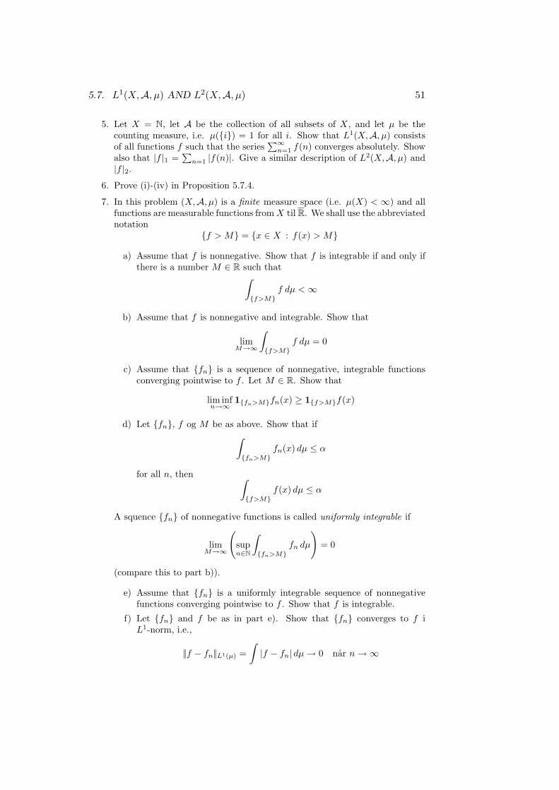
5.7. L1(X,A, µ) AND L2(X,A, µ) 51

5. Let X = N, let A be the collection of all subsets of X, and let µ be thecounting measure, i.e. µ(i) = 1 for all i. Show that L1(X,A, µ) consistsof all functions f such that the series

∑∞n=1 f(n) converges absolutely. Show

also that |f |1 =∑

n=1 |f(n)|. Give a similar description of L2(X,A, µ) and|f |2.

6. Prove (i)-(iv) in Proposition 5.7.4.

7. In this problem (X,A, µ) is a finite measure space (i.e. µ(X) < ∞) and allfunctions are measurable functions from X til R. We shall use the abbreviatednotation

f > M = x ∈ X : f(x) > M

a) Assume that f is nonnegative. Show that f is integrable if and only ifthere is a number M ∈ R such that∫

f>Mf dµ < ∞

b) Assume that f is nonnegative and integrable. Show that

limM→∞

∫f>M

f dµ = 0

c) Assume that fn is a sequence of nonnegative, integrable functionsconverging pointwise to f . Let M ∈ R. Show that

lim infn→∞

1fn>Mfn(x) ≥ 1f>Mf(x)

d) Let fn, f og M be as above. Show that if∫fn>M

fn(x) dµ ≤ α

for all n, then ∫f>M

f(x) dµ ≤ α

A squence fn of nonnegative functions is called uniformly integrable if

limM→∞

(supn∈N

∫fn>M

fn dµ

)= 0

(compare this to part b)).

e) Assume that fn is a uniformly integrable sequence of nonnegativefunctions converging pointwise to f . Show that f is integrable.

f) Let fn and f be as in part e). Show that fn converges to f iL1-norm, i.e.,

||f − fn||L1(µ) =∫|f − fn| dµ → 0 nar n →∞

measure and integration · originally, measure theory was the theory of the lebesgue measure, and...

Documents