me/ae455 mechanical vibrations and control conceptual and
TRANSCRIPT
1
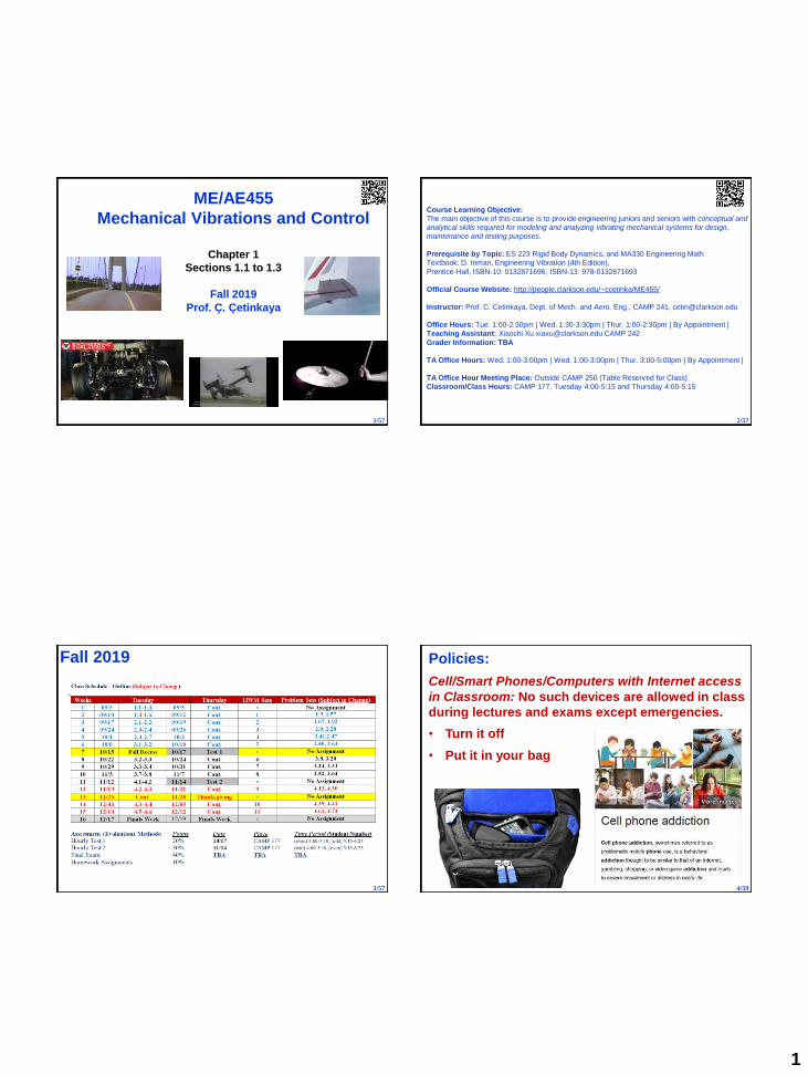
ME/AE455
Mechanical Vibrations and Control
Chapter 1
Sections 1.1 to 1.3
Fall 2019
Prof. Ç. Çetinkaya
1/57
Course Learning Objective:
The main objective of this course is to provide engineering juniors and seniors with conceptual and
analytical skills required for modeling and analyzing vibrating mechanical systems for design,
maintenance and testing purposes.
Prerequisite by Topic: ES 223 Rigid Body Dynamics, and MA330 Engineering Math
Textbook: D. Inman, Engineering Vibration (4th Edition),
Prentice-Hall, ISBN-10: 0132871696, ISBN-13: 978-0132871693
Official Course Website: http://people.clarkson.edu/~ccetinka/ME455/
Instructor: Prof. C. Cetinkaya, Dept. of Mech. and Aero. Eng., CAMP 241, [email protected]
Office Hours: Tue. 1:00-2:30pm | Wed. 1:30-3:30pm | Thur. 1:00-2:30pm | By Appointment |
Teaching Assistant: Xiaochi Xu [email protected] CAMP 242
Grader Information: TBA
TA Office Hours: Wed. 1:00-3:00pm | Wed. 1:00-3:00pm | Thur. 3:00-5:00pm | By Appointment |
TA Office Hour Meeting Place: Outside CAMP 250 (Table Reserved for Class)
Classroom/Class Hours: CAMP 177, Tuesday 4:00-5:15 and Thursday 4:00-5:15
2/57
Fall 2019
3/57 4/59
Policies:
Cell/Smart Phones/Computers with Internet access
in Classroom: No such devices are allowed in class
during lectures and exams except emergencies.
• Turn it off
• Put it in your bag
2
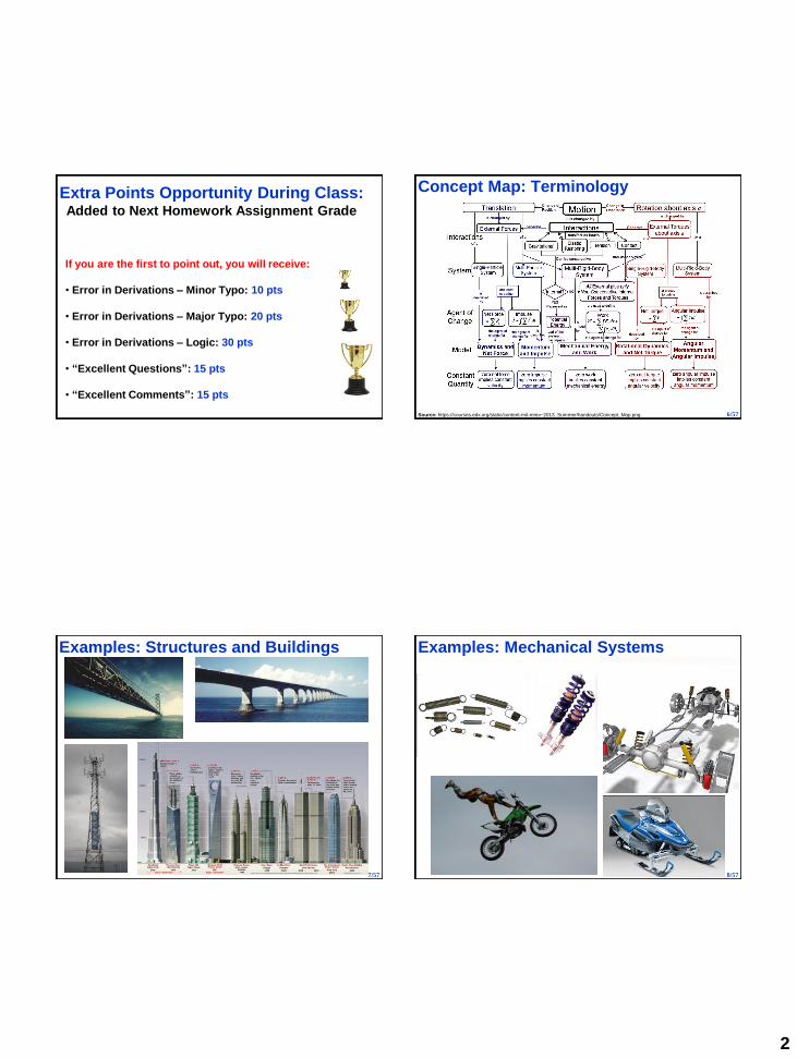
Extra Points Opportunity During Class:Added to Next Homework Assignment Grade
If you are the first to point out, you will receive:
• Error in Derivations – Minor Typo: 10 pts
• Error in Derivations – Major Typo: 20 pts
• Error in Derivations – Logic: 30 pts
• “Excellent Questions”: 15 pts
• “Excellent Comments”: 15 pts
Concept Map: Terminology
Source: https://courses.edx.org/static/content-mit-mrev~2013_Summer/handouts/Concept_Map.png 6/57
Examples: Structures and Buildings
7/57
Examples: Mechanical Systems
8/57
3
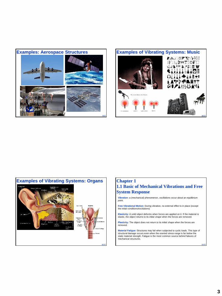
Examples: Aerospace Structures
9/57
Examples of Vibrating Systems: Music
10/57
Examples of Vibrating Systems: Organs
11/57
Chapter 1
1.1 Basic of Mechanical Vibrations and Free
System Response
Vibration: a (mechanical) phenomenon, oscillations occur about an equilibrium
point.
Free Vibrational Motion: During vibration, no external effect is in place (except
the initial conditions/excitations)
Elasticity: A solid object deforms when forces are applied on it. If the material is
elastic, the object returns to its initial shape when the forces are removed.
Plasticity: The object does not return to its initial shape when the forces are
removed.
Material Fatigue: Structures may fail when subjected to cyclic loads. This type of
structural damage occurs even when the exerted stress range is far below the
static material strength. Fatigue is the most common source behind failures of
mechanical structures.
12/57

4
Observation 01: Highway traffic light poles oscillating due to snow coverhttp://www.youtube.com/watch?v=xkOuPuawVeY
Observation 02: Vibrating flag pole
http://www.youtube.com/watch?v=bvLTErW5zNo
Observation 03: Vibration. See the unseen. (Fluke Corp.)
http://www.youtube.com/watch?v=W4s2UwKm7dc
Possible Questions:
1. What am I seeing/observing?
2. What is taking place? (engineering analysis)
3. Why is this occurring? (hypothesizing)
4. Am I missing something? (testing logical consequences of the hypothesis)
5. How can I apply this phenomenon to an engineering application? (commercial interest)
The scientific method requires observations of nature to formulate and test hypotheses.It consists
of these steps (wikipedia.org):
1. Asking a question about a natural phenomenon
2. Making observations of the phenomenon
3. Hypothesizing an explanation for the phenomenon
4. Predicting a logical consequence of the hypothesis
5. Testing the hypothesis by an experiment, an observational study, or a field study6. Creating a conclusion with data gathered in the experiment, or forming a revised/new hypothesis and
repeating the process
Direct Observations
13/57
Linear
Behavior
Nonlinearity
Consider a spring-mass system and perform a static
experiment: The spring is used to model elasticity in a system.
A plot of force versus displacement:
Linear Spring: A Thought Experiment
FBD:
From strength of materials, we know that:
kf k x Experiment
k
14/57
Free-body Diagram and an Equation of Motion of a System
0
0
( ) ( ) ( ) ( ) 0
(0)
(0)
k x t m x t m x t k x t
x x
x v
Newton’s Second Law of Motion (i.e. ΣF = m a) along x results in:
Second order ordinary
differential equation (ODE)
Generating an Equation of Motion
Free Body Diagram
15/57
Stiffness and MassVibration is caused by the interaction of two types of forces:
(i) Restitution Force: Related to position (stiffness) and
(ii) Inertia Force: Related to acceleration (mass, or mass distribution in
space)
Mass
m
k
x
Displacement (x)
Spring
Stiffness (k): Restitution Force
Mass (m): Inertia Force
Proportional to displacement
Proportional to acceleration
( )kf k x t static
( ) ( )mf m a t m x t dynamicO
Reference
Displacement
Coordinate
x
16/57
5
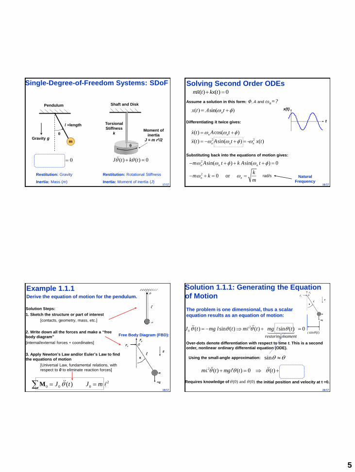
Single-Degree-of-Freedom Systems: SDoF
m
q
l =length
Pendulum
q(t) g
lq(t) 0
Gravity g
Shaft and Disk
q
( ) ( ) 0J t k tq q
Torsional
Stiffness
kMoment of
inertia
J = m r2/2
Restitution: Gravity
Inertia: Mass (m)
Restitution: Rotational Stiffness
Inertia: Moment of inertia (J)17/57
Solving Second Order ODEs
x(t) Asin(nt )
2 2
( ) cos( )
( ) sin( ) - ( )
n n
n n n
x t A t
x t A t x t
Assume a solution in this form: Φ, A and ωn=?
Differentiating it twice gives:
Substituting back into the equations of motion gives:
2
2
sin( ) sin( ) 0
0 or
n n n
n n
m A t k A t
km k
m
Natural
Frequency
t
x(t)
rad/s
( ) ( ) 0mx t kx t
18/57
Example 1.1.1
Solution Steps:
1. Sketch the structure or part of interest
[contacts, geometry, mass, etc.]
2. Write down all the forces and make a “free
body diagram”
[internal/external forces + coordinates]
3. Apply Newton’s Law and/or Euler’s Law to find
the equations of motion
[Universal Law, fundamental relations, with
respect to 0 to eliminate reaction forces]
Free Body Diagram (FBD):
2
0 0 0( ) J t J mq M
Derive the equation of motion for the pendulum.
19/57
The problem is one dimensional, thus a scalar
equation results as an equation of motion:
2
0 ( ) sin ( ) ( ) sin ( ) 0
restoring moment
J t mg l t m t mg tq q q q
Over-dots denote differentiation with respect to time t. This is a second
order, nonlinear ordinary differential equation (ODE).
2 ( ) ( ) 0 ( ) ( ) 0g
m t mg t t tq q q q
Requires knowledge of (0) and (0)q q the initial position and velocity at t =0.
Solution 1.1.1: Generating the Equation
of Motion
sinq qUsing the small-angle approximation:
sin ( )tq
20/57
6
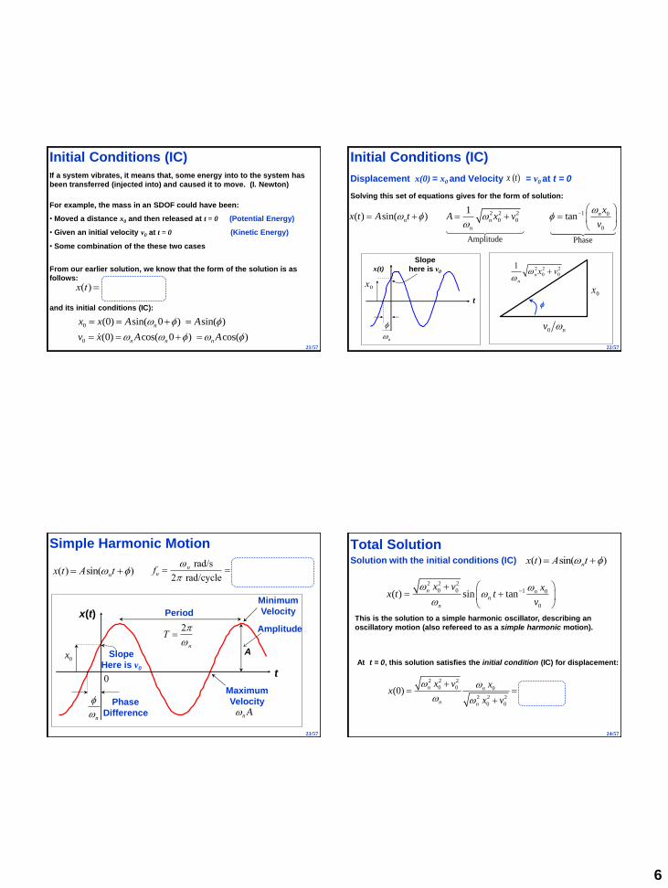
Initial Conditions (IC)
If a system vibrates, it means that, some energy into to the system has
been transferred (injected into) and caused it to move. (I. Newton)
0
0
(0) sin( 0 ) sin( )
(0) cos( 0 ) cos( )
n
n n n
x x A A
v x A A
From our earlier solution, we know that the form of the solution is as
follows:
For example, the mass in an SDOF could have been:
• Moved a distance x0 and then released at t = 0 (Potential Energy)
• Given an initial velocity v0 at t = 0 (Kinetic Energy)
• Some combination of the these two cases
x(t) Asin(nt )
and its initial conditions (IC):
21/57
Initial Conditions (IC)
Solving this set of equations gives for the form of solution:
2 2 2 1 00 0
0
Amplitude Phase
1( ) sin( ) tan n
n n
n
xx t A t A x v
v
x0
Displacement x(0) = x0 and Velocity = v0 at t = 0( )x t
0 nv
x0
1
n
n
2x0
2 v0
2
t
x(t)
Slope
here is v0
n
22/57
Simple Harmonic Motion
fn n rad/s
2 rad/cycle
n cycles
2 s
n
2Hz
Amplitude
t
x(t)
0x Slope
Here is v0
n
Period
T 2
n
Maximum
VelocityAn
x(t) Asin(nt )
Phase
Difference
A
23/57
0
Minimum
Velocity
Total Solution
2 2 2
0 0 1 0
0
( ) sin tann n
n
n
x v xx t t
v
This is the solution to a simple harmonic oscillator, describing an
oscillatory motion (also refereed to as a simple harmonic motion).
At t = 0, this solution satisfies the initial condition (IC) for displacement:
2 2 2
0 0 00
2 2 2
0 0
(0)n n
n n
x v xx x
x v
Solution with the initial conditions (IC) x(t) Asin(nt )
24/57
7
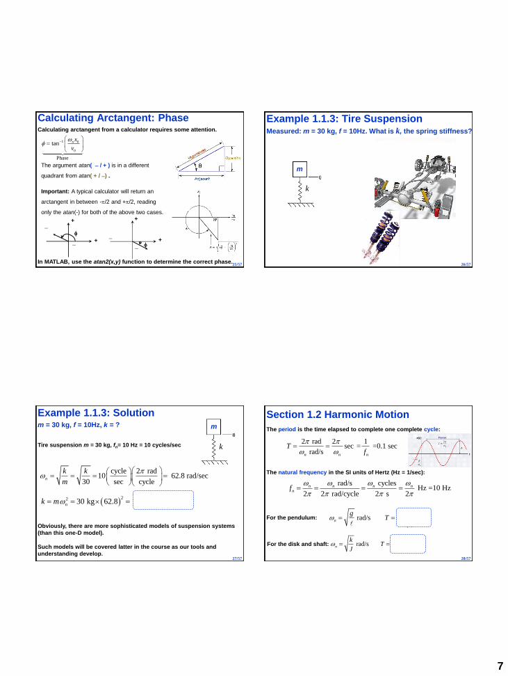
In MATLAB, use the atan2(x,y) function to determine the correct phase.
Calculating Arctangent: Phase
+
+
_
+
+
Calculating arctangent from a calculator requires some attention.
The argument atan( ̶ / + ) is in a different
quadrant from atan( + / ̶ ) .
Important: A typical calculator will return an
arctangent in between -/2 and +/2, reading
only the atan(-) for both of the above two cases.
_
__
1 0
0
Phase
tan n x
v
25/57
Example 1.1.3: Tire Suspension Measured: m = 30 kg, f = 10Hz. What is k, the spring stiffness?
k
m
26/57
Example 1.1.3: Solution
22 530 kg 62.8 1.184 10 N/mnk m
Obviously, there are more sophisticated models of suspension systems
(than this one-D model).
Such models will be covered latter in the course as our tools and
understanding develop.
m = 30 kg, f = 10Hz, k = ?
Tire suspension m = 30 kg, fn= 10 Hz = 10 cycles/sec
cycle 2 rad10 62.8 rad/sec
30 sec cyclen
k k
m
k
m
27/57
Section 1.2 Harmonic Motion
2 rad 2 1 sec = =0.1 sec
rad/sn n n
Tf
The natural frequency in the SI units of Hertz (Hz = 1/sec):
The period is the time elapsed to complete one complete cycle:
rad/s cycles Hz =10 Hz
2 2 rad/cycle 2 s 2
n n n nnf
For the pendulum: rad/s 2 secn
gT
g
rad/s 2 secn
k JT
J k For the disk and shaft:
28/57
8
Note how the relative magnitude of each increases with n for n > 1
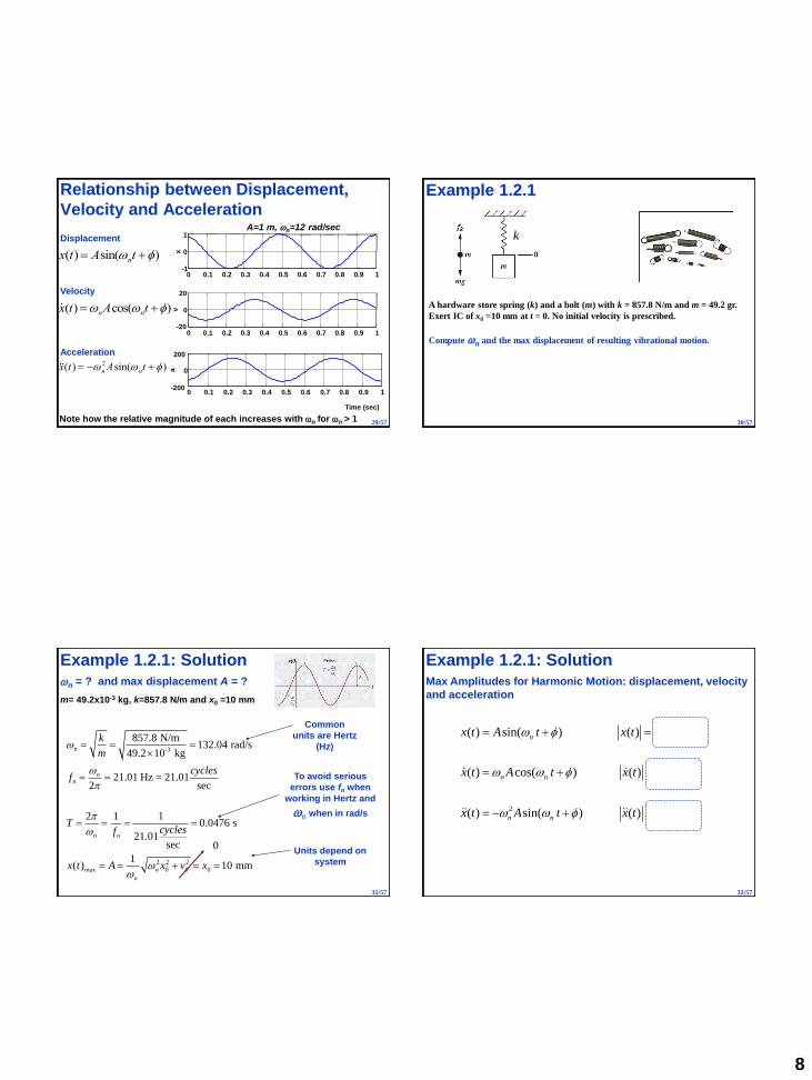
Relationship between Displacement,
Velocity and Acceleration
0 0.1 0.2 0.3 0.4 0.5 0.6 0.7 0.8 0.9 1-200
0
200
Time (sec)
a
0 0.1 0.2 0.3 0.4 0.5 0.6 0.7 0.8 0.9 1-1
0
1
x
A=1 m, n=12 rad/sec
x(t) Asin(nt )
x(t) nAcos(nt )
x(t) n
2Asin(nt )
Displacement
Velocity
Acceleration
0 0.1 0.2 0.3 0.4 0.5 0.6 0.7 0.8 0.9 1-20
0
20
v
29/57
Example 1.2.1
A hardware store spring (k) and a bolt (m) with k = 857.8 N/m and m = 49.2 gr.
Exert IC of x0 =10 mm at t = 0. No initial velocity is prescribed.
Compute n and the max displacement of resulting vibrational motion.
k
30/57
Example 1.2.1: Solution
-3
2 2 2
max 0 0 0
857.8 N/m132.04 rad/s
49.2 10 kg
21.01 Hz = 21.012 sec
2 1 10.0476 s
21.01sec
1( ) 10 mm
n
nn
n n
n
n
k
m
cyclesf
Tcyclesf
x t A x v x
0
Common
units are Hertz
(Hz)
To avoid serious
errors use fn when
working in Hertz and
n when in rad/s
Units depend on
system
m= 49.2x10⁻³ kg, k=857.8 N/m and x0 =10 mm
n = ? and max displacement A = ?
31/57
2 2
( ) sin( ) ( )
( ) cos( ) ( )
( ) sin( ) ( )
n
n n n
n n n
x t A t x t A
x t A t x t A
x t A t x t A
Example 1.2.1: SolutionMax Amplitudes for Harmonic Motion: displacement, velocity
and acceleration
32/57

9
max
2 3 2
max
2
1 0
( ) 1320.4 mm/s=1.32 m/s
( ) 174.35 10 mm/s
=174.35 m/s 17.8
tan rad0 2
( ) 10 sin(132.04 / 2) 10 cos(132.4 ) mm
n
n
n
v t A
a t A
g
x
x t t t
g = 9.8 m/s2
2.92 mph
90°
~0.4 in max = A
Example 1.2.1: SolutionMax Amplitudes
33/57
Does Gravity Matter in Spring Problems?
Let be the deflection caused by hanging a mass on a spring
( = x1 - x0 in the figure)
Then from static equilibrium:
m g k
Next sum the forces in the vertical for some point x > x1 measured
From the equilibrium position
0
( ) ( ) 0
m x k x m g k x m g k
m x t k x t
So no, gravity does not have an effect on the vibration
(note that this is not the case if the spring is nonlinear)
Reference
34/57
Example 1.2.2
A 2 m pendulum swings with a period of 2.893 s. What is the acceleration
due to gravity at that locality? Namely, g = ?
Pendulums and Measuring the gravitational acceleration g
m
q
l =length
Gravity g
Reference
35/57
Example 1.2.2: Solution
2 2
2 2 2
2
4 42 m
2.893 s
= 9.434 m/s
gT
g
T = 2.893 sec, l = 2m
m
q
l =length
q(t) g
lq(t) 0
Gravity g 2
n
T
rad/s, 2 sn
gT
g
36/57
10
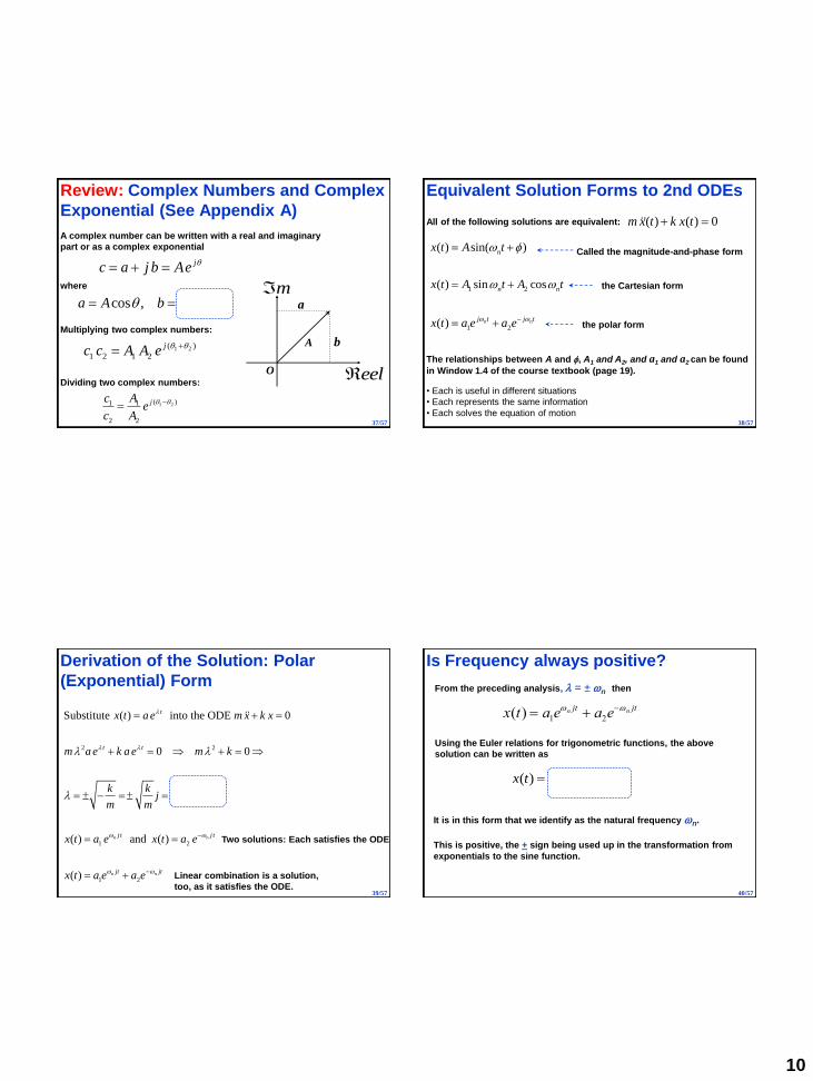
Review: Complex Numbers and Complex
Exponential (See Appendix A)
eel
m
b
a
A
jc a j b Ae q
A complex number can be written with a real and imaginary
part or as a complex exponential
where
cos , sina A b Aq q
Multiplying two complex numbers:
1 2( )
1 2 1 2
jc c A A e
q q
Dividing two complex numbers:
1 2( )1 1
2 2
jc Ae
c A
q q
O
37/57
Equivalent Solution Forms to 2nd ODEs
1 2
1 2
( ) sin( )
( ) sin cos
( ) n n
n
n n
j t j t
x t A t
x t A t A t
x t a e a e
All of the following solutions are equivalent:
The relationships between A and , A1 and A2, and a1 and a2 can be found
in Window 1.4 of the course textbook (page 19).
the Cartesian form
Called the magnitude-and-phase form
the polar form
• Each is useful in different situations
• Each represents the same information
• Each solves the equation of motion
( ) ( ) 0m x t k x t
38/57
Derivation of the Solution: Polar
(Exponential) Form
2 2
1 2
1 2
Substitute ( ) into the ODE 0
0 0
( ) and ( )
( )
n n
n n
t
t t
n
j t j t
jt jt
x t a e m x k x
m a e k a e m k
k kj j
m m
x t a e x t a e
x t a e a e
Two solutions: Each satisfies the ODE
Linear combination is a solution,
too, as it satisfies the ODE.39/57
Is Frequency always positive?
x(t) a1en jt a2e
n jt
( ) sin nx t A t
From the preceding analysis, = ± n then
Using the Euler relations for trigonometric functions, the above
solution can be written as
It is in this form that we identify as the natural frequency n.
This is positive, the + sign being used up in the transformation from
exponentials to the sine function.
40/57
11
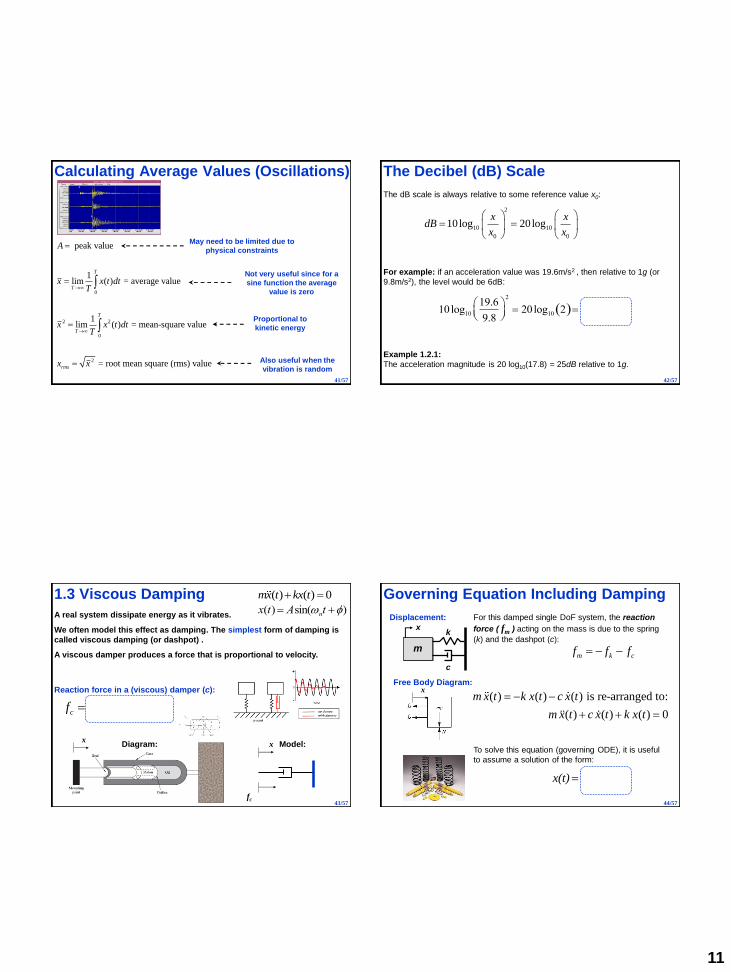
Calculating Average Values (Oscillations)
0
2 2
0
2
peak value
1lim ( ) = average value
1lim ( ) = mean-square value
= root mean square (rms) value
T
T
T
T
rms
A
x x t dtT
x x t dtT
x x
Proportional to
kinetic energy
Not very useful since for a
sine function the average
value is zero
May need to be limited due to
physical constraints
Also useful when the
vibration is random
41/57
Example 1.2.1:
The acceleration magnitude is 20 log10(17.8) = 25dB relative to 1g.
The Decibel (dB) Scale
The dB scale is always relative to some reference value x0:
2
10 10
0 0
10log 20log x x
dBx x
For example: if an acceleration value was 19.6m/s2 , then relative to 1g (or
9.8m/s2), the level would be 6dB:
10log10
19.6
9.8
2
20log10 2 6dB
42/57
1.3 Viscous Damping
A real system dissipate energy as it vibrates.
We often model this effect as damping. The simplest form of damping is
called viscous damping (or dashpot) .
A viscous damper produces a force that is proportional to velocity.
Reaction force in a (viscous) damper (c):
( ) ( )cf c v t c x t
x
fc
x
x(t) Asin(nt )
( ) ( ) 0mx t kx t
Model:Diagram:
43/57
Governing Equation Including Damping
m
kx
Displacement:
c
For this damped single DoF system, the reaction
force ( fm ) acting on the mass is due to the spring
(k) and the dashpot (c):
To solve this equation (governing ODE), it is useful
to assume a solution of the form:
tx(t) a e
Free Body Diagram:x
m k cf f f
( ) ( ) ( ) is re-arranged to:
( ) ( ) ( ) 0
m x t k x t c x t
m x t c x t k x t
44/57
12
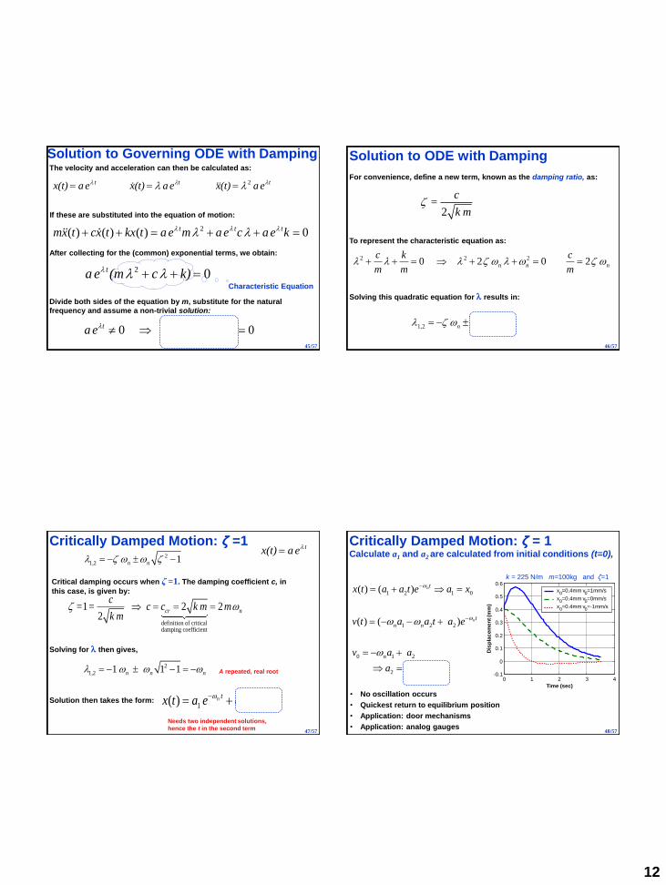
Solution to Governing ODE with Damping
2 t t tx(t) a e x(t) a e x(t) a e
2 0 ta e (m c k)
The velocity and acceleration can then be calculated as:
If these are substituted into the equation of motion:
Divide both sides of the equation by m, substitute for the natural
frequency and assume a non-trivial solution:
20 0t c ka e
m m
Characteristic Equation
2( ) ( ) ( ) 0 t t tmx t cx t kx t a e m a e c a e k
After collecting for the (common) exponential terms, we obtain:
45/57
Solution to ODE with Damping
2 2 20 2 0 2n n n
c k c
m m m
For convenience, define a new term, known as the damping ratio, as:
To represent the characteristic equation as:
Solving this quadratic equation for results in:
2
c=
k m
2
1 2 1, n n
46/57
Critically Damped Motion: ζ =1
definition of criticaldamping coefficient
=1 2 22
cr n
c= c c k m m
k m
Critical damping occurs when ζ =1. The damping coefficient c, in
this case, is given by:
Solution then takes the form:
Solving for then gives,
2
1 2 1 1 1, n n n A repeated, real root
1 2( ) n nt tx t a e a t e
Needs two independent solutions,
hence the t in the second term
2
1 2 1, n n
tx(t) a e
47/57
Critically Damped Motion: ζ = 1Calculate a1 and a2 are calculated from initial conditions (t=0),
1 2 1 0
1 2 2
0 1 2
2 0 0
( ) ( )
( ) ( )
n
n
t
t
n n
n
n
x t a a t e a x
v t a a t a e
v a a
a v x
0 1 2 3 4
-0.1
0
0.1
0.2
0.3
0.4
0.5
0.6
Time (sec)
Dis
pla
cem
en
t (m
m)
x0=0.4mm v
0=1mm/s
x0=0.4mm v
0=0mm/s
x0=0.4mm v
0=-1mm/s
• No oscillation occurs
• Quickest return to equilibrium position
• Application: door mechanisms
• Application: analog gauges
k = 225 N/m m=100kg and ζ=1
48/57
13
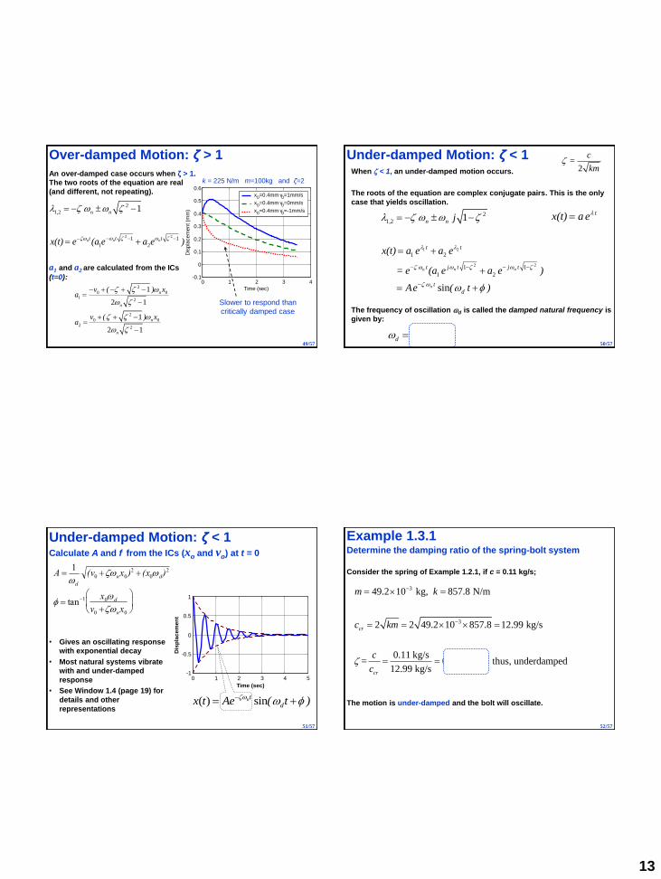
Over-damped Motion: ζ > 1
An over-damped case occurs when ζ > 1.
The two roots of the equation are real
(and different, not repeating).
2 2
2
1 2
1 1
1 2
1
n nn
, n n
t ttx(t) e (a e a e )
a1 and a2 are calculated from the ICs
(t=0):
2
0 01
2
2
0 0
22
1
2 1
1
2 1
n
n
n
n
v ( ) xa
v ( ) xa
0 1 2 3 4-0.1
0
0.1
0.2
0.3
0.4
0.5
0.6
Time (sec)
Dis
pla
cem
en
t (m
m)
k = 225 N/m m=100kg and ζ=2
x0=0.4mm v
0=1mm/s
x0=0.4mm v0=0mm/s
x0=0.4mm v
0=-1mm/s
Slower to respond than
critically damped case
49/57
Under-damped Motion: ζ < 1When < 1, an under-damped motion occurs.
The roots of the equation are complex conjugate pairs. This is the only
case that yields oscillation.
1 2
2 2
2
1 2
1 2
1 1
1 2
1
=
sin
n nn
n
, n n
t t
j t j tt
t
d
j
x(t) a e a e
e (a e a e )
Ae ( t )
The frequency of oscillation d is called the damped natural frequency is
given by:
21 d n
2
c=
km
tx(t) a e
50/57
Under-damped Motion: ζ < 1Calculate A and f from the ICs (xo and vo) at t = 0
A 1
d
(v0 nx0)2 (x0d)
2
tan1 x0d
v0 nx0
0 1 2 3 4 5-1
-0.5
0
0.5
1
Time (sec)
Dis
pla
ce
me
nt
• Gives an oscillating response
with exponential decay
• Most natural systems vibrate
with and under-damped
response
• See Window 1.4 (page 19) for
details and other
representations( ) sinnt
dx t Ae ( t )
51/57
Example 1.3.1
3
3
49.2 10 kg, 857.8 N/m
2 2 49.2 10 857.8 12.99 kg/s
0.11 kg/s= 0.0085 1 thus, underdamped
12.99 kg/s
cr
cr
m k
c km
c
c
Consider the spring of Example 1.2.1, if c = 0.11 kg/s;
The motion is under-damped and the bolt will oscillate.
Determine the damping ratio of the spring-bolt system
52/57
14
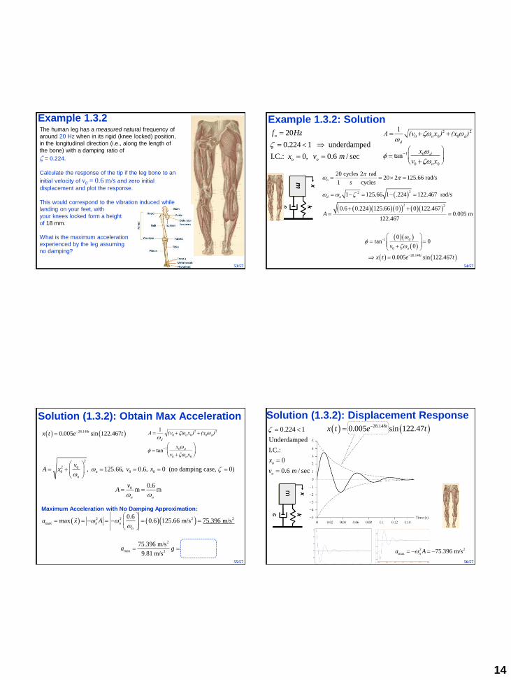
Example 1.3.2The human leg has a measured natural frequency of
around 20 Hz when in its rigid (knee locked) position,
in the longitudinal direction (i.e., along the length of
the bone) with a damping ratio of
= 0.224.
Calculate the response of the tip if the leg bone to an
initial velocity of v0 = 0.6 m/s and zero initial
displacement and plot the response.
This would correspond to the vibration induced while
landing on your feet, with
your knees locked form a height
of 18 mm.
What is the maximum acceleration
experienced by the leg assuming
no damping?
53/57
Example 1.3.2: Solution
22
2 2
-1
0
28.148
20 cycles 2 rad20 2 125.66 rad/s
1 cycles
1 125.66 1 .224 122.467 rad/s
0.6 0.224 125.66 0 0 122.4670.005 m
122.467
0tan 0
0
0.005
n
d n
d
n
t
s
A
v
x t e
sin 122.467t
20
0.224 1 underdamped
I.C.: 0, 0.6 / sec
n
o o
f Hz
x v m
A 1
d
(v0 nx0)2 (x0d)
2
tan1 x0d
v0 nx0
54/57
Solution (1.3.2): Obtain Max Acceleration
2
2 00 0 0
0
2 2 2 2
max
, 125.66, 0.6, 0 (no damping case, 0)
0.6m m
0.6max 0.6 125.66 m/s 75.396 m/s
n
n
n n
n n
n
vA x v x
vA
a x A
Maximum Acceleration with No Damping Approximation:
2
max 2
75.396 m/s7.68g
9.81 m/sa g
28.1480.005 sin 122.467tx t e t
A 1
d
(v0 nx0)2 (x0d)
2
tan1 x0d
v0 nx0
55/57
Solution (1.3.2): Displacement Response
28.1480.005 sin 122.47tx t e t
2 2
max 75.396 m/sna A
0.224 1
Underdamped
I.C.:
0
0.6 / sec
o
o
x
v m
56/57
15
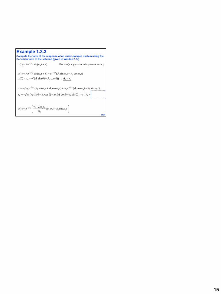
Example 1.3.3
1 2
0
0 1 2 2 0
1 2 1 2
0
( ) sin( ) Use sin( ) sin sin cos cos
( ) sin( ) ( sin cos )
(0) ( sin(0) cos(0))
( sin cos ) ( cos sin )
n
n n
n n
t
d
t t
d d d
t t
n d d d d d
x t Ae t x y x y x y
x t Ae t e A t A t
x x e A A A x
x e A t A t e A t A t
v
0 01 0 1 0 1
0 00
( sin 0 cos 0) ( cos 0 sin 0)
( ) sin cosn
nn d
d
t nd d
d
v xA x A x A
v xx t e t x t
Compute the form of the response of an under-damped system using the
Cartesian form of the solution (given in Window 1.5.)
57/57