mcnp5 and geant4 comparisons for preliminary fast …
TRANSCRIPT

MCNP5 AND GEANT4 COMPARISONS FOR PRELIMINARY FAST NEUTRON
PENCIL BEAM DESIGN AT THE UNIVERSITY OF UTAH TRIGA SYSTEM
by
Christian Amevi Adjei
A thesis submitted to the faculty of The University of Utah
in partial fulfillment of the requirements for the degree of
Master of Science
in
Nuclear Engineering
Department of Civil and Environmental Engineering
University of Utah
December 2012

Copyright © Christian Amevi Adjei 2012
All Rights Reserved

The University of Utah Graduate School
STATEMENT OF THESIS APPROVAL
The thesis of _______________________Christian Amevi Adjei____________________
has been approved by the following supervisory committee members:
_____________ Tatjana Jevremovic______________ , Chair 10/25/2012Date Approved
_______________ Dong-Ok Choe________________ , Member 10/25/2012Date Approved
_________________Haori Yang__________________ , Member 10/25/2012Date Approved
and by _____________________ Chris Pantelides_____________________ , Chair of
the Department of _____________ Civil and Environmental Engineering
and by Charles A. Wight, Dean of The Graduate School.

ABSTRACT
The main objective of this thesis is twofold. The starting objective was to
develop a model for meaningful benchmarking of different versions of GEANT4
against an experimental set-up and MCNP5 pertaining to photon transport and
interactions. The following objective was to develop a preliminary design of a Fast
Neutron Pencil Beam (FNPB) Facility to be applicable for the University of Utah
research reactor (UUTR) using MCNP5 and GEANT4. The three various GEANT4
code versions, GEANT4.9.4, GEANT4.9.3, and GEANT4.9.2, were compared to
MCNP5 and the experimental measurements of gamma attenuation in air. The
average gamma dose rate was measured in the laboratory experiment at various
distances from a shielded cesium source using a Ludlum model 19 portable NaI
detector. As it was expected, the gamma dose rate decreased with distance. All three
GEANT4 code versions agreed well with both the experimental data and the MCNP5
simulation. Additionally, a simple GEANT4 and MCNP5 model was developed to
compare the code agreements for neutron interactions in various materials.
Preliminary FNPB design was developed using MCNP5; a semi-accurate
model was developed using GEANT4 (because GEANT4 does not support the reactor
physics modeling, the reactor was represented as a surface neutron source, thus a
semi-accurate model). Based on the MCNP5 model, the fast neutron flux in a
sample holder of the FNPB is obtained to be 6.52x10⁷ n/cm2s, which is one order of
magnitude lower than gigantic fast neutron pencil beam facilities existing

elsewhere. The MCNP5 model-based neutron spectrum indicates that the maximum
expected fast neutron flux is at a neutron energy of ~1 MeV. In addition, the MCNP5
model provided information on gamma flux to be expected in this preliminary FNPB
design; specifically, in the sample holder, the gamma flux is to be expected to be
around 108 i/cm2s, delivering a gamma dose of 4.54x10³ rem/hr. This value is one to
two orders of magnitudes below the gamma exposure as exists in the currently used
fast neutron irradiation facility at the UUTR. The GEANT4.9.4 semi-accurate model
of the FNPB design provided higher values for neutron and gamma fluxes,
indicating the importance of transfering the data from MCNP5 rather than using
the GEANT4 default neutron spectra.
iv

CONTENTS
ABSTRACT.................................................................................................................... iii
LIST OF FIGURES...................................................................................................... vii
LIST OF TABLES.......................................................................................................... ix
ACKNOWLEDGEMENTS ............................................................................................ x
Chapters
1. INTRODUCTION....................................................................................................... 1
1.1. Motivation............................................................................................................ 11.2. Thesis Objectives ................................................................................................. 11.3. Organization of the Thesis.................................................................................. 2
2. BASICS ON GEANT4 AND MCNP5 CODES........................................................... 4
2.1. GEANT4 Code...................................................................................................... 42.1.1. Applications of GEANT4............................................................................... 52.1.2. GEANT4 Physics Models.............................................................................. 52.1.3. GEANT4 Functionality................................................................................. 92.1.4. GEANT4 Benchmark and Accuracy........................................................... 11
2.2. MCNP5 Code...................................................................................................... 122.2.1. Applications of MCNP5............................................................................... 132.2.2. MCNP5 Physics Processes.......................................................................... 142.2.3. MCNP5 Functionality................................................................................. 152.2.4. MCNP5 Benchmark and Accuracy............................................................. 16
2.3. Summary of GEANT4 and MCNP5 Similarities and Differences...................18
3. EXPERIMENTAL ASSESSMENT OF DIFFERENT GEANT4 CODE VERSIONS AND COMPARISON TO MCNP5............................................................................... 20
3.1. Description of Experiment to Benchmark GEANT4 and MCNP5.................. 203.2. Modeling of Gamma Interactions in GEANT4 and MCNP5...........................23
3.2.1. Modeling of Gamma Interactions in GEANT4.......................................... 233.2.2. Modeling of Gamma Interactions in MCNP5............................................ 27
3.3. Experiment Assessment of Gamma Interactions Modeling using GEANT4 and MCNP5...................................................................................................................... 29
4. BASICS ON FAST NEUTRON PENCIL BEAM FACILITY 35

4.1. About Fast Neutrons......................................................................................... 354.2. Fast Neutron Facilities...................................................................................... 37
4.2.1. Application of Fast Neutron Facilities....................................................... 384.2.2. Application of Fast Neutron Pencil Beam Facilities................................. 41
5. PRELIMINARY DESIGN OF THE FAST NEUTRON PENCIL BEAM FACILITY AT THE UNIVERSITY OF UTAH TRIGA (UUTR)................................................... 44
5.1. General Characteristics of the UUTR............................................................... 445.2. Conceptual Design of the Fast Neutron Pencil Beam Facility at the UUTR ..465.3. MCNP5 Model of the Fast Neutron Pencil Beam Facility at the UUTR........555.4. GEANT4 Model of the Fast Neutron Pencil Beam Facility at the UUTR......575.5 Comparison of GEANT4 and MCNP5 in Modeling Neutron Interactions.......575.6. Comparison between MCNP5 and GEANT4.9.4 Models of the Fast NeutronPencil Beam Facility at the UUTR.......................................................................... 625.7 Comparison of UUTR FNPB design with other fast neutron pencil beam facilities ..................................................................................................................... 69
6. CONCLUSION AND FUTURE WORK................................................................... 71
6.1. Conclusion.......................................................................................................... 716.2. Recommendations for Future Work.................................................................. 73
Appendices
A. MCNP5 INPUT FILE FOR PHOTON EXPERIMENT...................................... 75
B. GEANT4.9.4 INPUT FILE FOR PHOTON EXPERIMENT.............................. 79
C. MCNP5 INPUT FILE FOR NEUTRON INTERACTION.................................. 84
D. GEANT4.9.4 INPUT FILE FOR NEUTRON INTERACTION.......................... 87
E. MCNP5 INPUT FILE OF UUTR FNPB............................................................. 92
F. GEANT4.9.4 INPUT FILE OF UUTR FNPB................................................... 107
REFERENCES........................................................................................................... 117
vi
LIST OF FIGURES
2-1 Applications of GEANT4..................................................................................... 6
2-2 GEANT4 class categories...................................................................................10
2-3 Applications of MCNP5..................................................................................... 13
2-4 MCNP5 categories............................................................................................ 16
3-1 137Cs decay scheme............................................................................................ 20
3-2 Diagram of cesium source in Pig shielding ..................................................... 22
3-3 Block diagram of the experimental set-up at UNEP facitly (MEB1205)........ 23
3-4 Comparison of GEANT4.9.2, GEANT4.9.3 and GEANT4.9.4 gamma dose rateas a function of distance from the source ....................................................... 33
3-5 Comparison of gamma dose rate as a function of distance from the source between the measured and calculated values using GEANT4 and MCNP5 . 33
4-1 Classification of neutron energies and interactions.......................................36
5-1 Cross section diagram of the UUTR 100-kWt TRIGA research reactor........45
5-2 Vertical cross-section diagram of FNIF............................................................ 47
5-3 Outline of UUTR reactor and FNIF.................................................................. 47
5-4 UUTR FNPB model........................................................................................... 48
5-5 Cross-section plots of aluminum, A l................................................................. 49
5-6 Cross-section plots of boron, B-10..................................................................... 51
5-7 Cross-section plots of graphite, C ..................................................................... 51
5-8 Cross-section plots of lead, Pb............................................................................52
5-9 Cross-section plots of Hydrogen, H ................................................................... 53
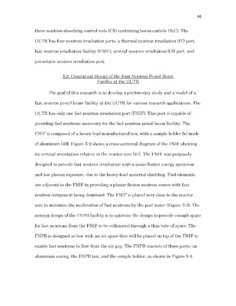
5-10 Model of aluminum casing and FNPB sample holder..................................... 54
5-11 Cross-section model of UUTR FNPB................................................................ 55
5-12 MCNP5 3-D model of UUTR FNPB.................................................................. 56

5-13 MCNP5 cross section view of UUTR FNPB..................................................... 56
5-14 GEANT4 model of UUTR FNPB........................................................................58
5-15 GEANT4 and MCNP5 simulation of neutron interaction with boron-10....... 59
5-16 GEANT4 and MCNP5 simulation of neutron interaction with lead............... 60
5-17 GEANT4 and MCNP5 simulation of neutron interaction with paraffin........ 61
5-18 MCNP5 - Neutron spectrum of UUTR FNPB.................................................. 64
5-19 MCNP5 - Gamma spectrum of UUTR FNPB................................................... 67
5-20 Comparison of UUTR FNPB spectrum with literature................................... 70
viii

LIST OF TABLES
2-1 Electromagnetic interactions as modeled in GEANT4..................................... 8
3-1 Background dose rate at various distance around experimental area..........30
3-2........ GEANT4 and MCNP dose rate in comparison to experimental measurements ........................................................................................................................... 34
3-3 Percentage difference of experimental measurements with GEANT4 and MCNP5 simulations.......................................................................................... 34
4-1 Applications of fast neutron facilities.............................................................. 38
4-2 Fast Neutron Therapy (FNT) facilities around the world..............................42
5-1 MCNP5 and GEANT4 comparison of neutron interactions ..........................62
5-2 MCNP reactor physics neutron simulation of UUTR FNPB.......................... 63
5-3 MCNP neutron flux simulation of UUTR FNPB............................................ 65
5-4 MCNP reactor physics gamma simulation of UUTR FNPB........................... 66
5-5 MCNP gamma flux simulation of UUTR FNPB............................................. 66
5-6 GEANT4 summary of UUTR FNPB simulation............................................. 68
5-7 GEANT4 simulation of neutron and gamma fluence in the UUTR FNPB 68
5-8 Comparison of MCNP5 and GEANT4.9.4 simulation of UUTR FNPB.........69

ACKNOWLEDGEMENTS
Foremost, glory and honour to God, for the opportunity given me to take up
this study. I am indebted to my advisor, Professor Tatjana Jevremovic, for her
unconditional guidance, advice, support, and opportunities she has provided for my
academic development in my graduate studies. Sincere gratitude to Professor Dong-
Ok Choe and Professor Haori Yang for their support and guidance. I would like to
express my gratitude to Dr. Hermilo Hernandez for his support and encouragement.
Also, I would like to thank my colleagues and friends, Avdo Cutic, Andrey Rybalkin,
Can Liao, Philip Babitz, Todd Sherman, Jason Rapich, and Chris Dances, for their
help and support. Finally, my heartfelt gratitude to my parents (Andrew A. Adjei
and Cecilia Adjei), my siblings (Rose Siedu and Andrew Adjei Jr.), brother in-law
(Frederick Siedu), nephew (Joshua Anglamaga), and nieces (Nomu Anglamaga,
Zunou Anglamaga, and Pupil Anglama), for their prayers and support.

CHAPTER 1
INTRODUCTION
1.1. Motivation
The University of Utah TRIGA Reactor (UUTR) is licensed to operate at a
maximum power of 100 kW, and it is used for research, teaching, and training. The
UUTR has four neutron irradiation ports used for a number of applications, such as,
but not limited to: Neutron Activation Analysis (NAA), irradiation of samples,
cadmium ratio measurements, studies on irradiation damage to materials, effects of
radiation on some electronic components, and basic studies on biological effects of
radiation. Currently, the UUTR has no Fast Neutron Pencil Beam (FNPB)
irradiation port. Design and installation of such a facility would open up a variety of
new applications, such as fast neutron irradiation studies to understand the effect of
fast neutrons on biological cells, by-standard effects, impact on materials and
nanoparticles, as well as for benchmarking numerical simulations based on various
codes, such as, for example, GEANT4 and MCNP5/X.
1.2. Thesis Objectives
The main objective of this thesis is to develop a preliminary design of the
Fast Neutron Pencil Beam facility and assess the feasibility of its installation in the
UUTR pool. In order to develop such a design, two known codes used in the nuclear
industry are adopted; GEANT4 [1] and MCNP5/X [2]. The MCNP5 code was

developed, and continues to be modified, in the United States; the GEANT4 code
was developed, and continues to be modified, in Europe. Both codes are based on the
Monte Carlo method for tracking particles in the geometry of interest. GEANT4,
being an open software code, suffered numerous changes, so that now, a number of
subversions are available with no clear understanding of the accuracy of each
subversion. MCNP5/X is closed to public domain and therefore, its accuracy is
strictly controlled and tracked with every new code version. Therefore, in order to
understand what the best subversion of GEANT4 code is, a few comparisons were
performed developing experimental and numerical examples.
Detailed objectives of this thesis are summarized as follows:
1. Perform experimental assessment to validate different versions of the
GEANT4 code and compare it to MCNP5 focusing at photon
transport and interactions.
2. Compare MCNP5/X and GEANT4 in modeling neutron transport in
various media.
3. Design a preliminary model of a Fast Neutron Pencil Beam facility at
the UUTR using MCNP5/X and GEANT4.
1.3. Organization of the Thesis
The basic description of GEANT4 and MCNP5, similarities, and differences
are provided in Chapter 2. In Chapter 3, the experimental assessment of gamma
interactions using different GEANT4 code versions in comparison to MCNP5 are
described. The basics of a Fast Neutron Pencil Beam facility are described in
2

3
Chapter 4. In Chapter 5, the preliminary design of a fast neutron irradiation facility
at the University of Utah TRIGA (UUTR) is described. The comparison of MCNP5
and GEANT4 models of the preliminary design of the fast neutron pencil beam are
also evaluated. Chapter 6 outlines the future work and conclusion of this research
study.

CHAPTER 2
BASICS ON GEANT4 AND MCNP5 CODES
2.1. GEANT4 Code
GEANT4 is a Monte Carlo-based code that is a successor of GEANT3
developed in two independent studies at CERN and KEK in 1993 [1]. Both groups
researched how modern computing techniques could be applied to improve existing
FORTRAN-based GEANT3 simulation programs, and finally developed GEANT4 in
1994. The main objective of developing the GEANT4 code was to have a simulation
program which had the flexibility and functionality to meet the essentials and needs
of subatomic physics experiments. The development of GEANT4 has grown to
become a large international collaboration of over hundred (100) scientist, physicist
programmers, and software engineers from a number of institutions and universities
participating in a wide range of research experiments in Europe, Japan, Canada,
and the United States [3].
GEANT4 is a modern object oriented (OO) environment code based on C++
that exploits advanced software-engineering techniques and object-oriented
technology to achieve transparency. GEANT4 is one of the largest and most
ambitious open source codes in terms of the size and scope. Every section of the
GEANT4 code is individually managed by a group of experts known as the
international GEANT4 collaboration group. In addition, there is a working group for
testing, quality assurance, software management, and documentation of the

5
software. The GEANT4 code is freely available, accompanied by an installation
guide and an extensive set of documentation [1, 3].
2.1.1. Applications of GEANT4
GEANT4 is a software toolkit based on Monte Carlo simulation of particle
transport and interaction with matter. One of the GEANT4 code’s powerful
applications is its use in instrumentation studies of the High Energy Physics (HEP),
and Large Hadron Collider (LHC) experiment [4], simulation of the BaBar
experiment [5], large HEP experiments ATLAS [4, 5], among others. GEANT4 users
come from a variety of fields, including space and radiation science, medical science,
and technology transfer, which basically allows the user to incorporate other
subroutine programs from other simulation codes into GEANT4 (Figure 2-1).
Specifically, the interest from the space and medical communities stems from the
following aspects of the toolkit [6, 7]: freely available software with long-term
support, object-oriented design and component approach, a wide choice of geometry
shapes, geometry and tracks visualization, particle tracking in fields, and a rich set
of physics models. GEANT4 provides users the ability to construct stand-alone
applications built upon another object-oriented framework.
2.1.2. GEANT4 Physics Models
GEANT4 consist of a number of various physics models supporting the
interactions of particles with matter across a wide range of energies. It provides the
user with interfaces, built-in steering routines, and commands at every level of
simulation.

6
Figure 2-1. Applications of GEANT4. Adapted from [1]
A limitation with older versions of the GEANT4 was the difficulty of adding new
physics models, due to the complexity and interdependence of physics procedures
which are “hard coded” into the code. In contrast, the object-oriented approach
helped manage complexity and limit dependencies by defining a uniform interface
and common organizational principles used for all physics models. Within the
GEANT4, the functionality of models can easily be recognized and understood,
making the creation and addition of new physics models easy and well defined [3-5].
All aspects of the simulation process that can be included in the code are:
geometry of a system to be modeled, materials, particles of interest, generation of
primary events, tracking of particles, physics processes governing particle
7
interactions, storage of events and tracks, visualization of the detector and particle
trajectories, and analysis of simulation data [7, 8, 9]. GEANT4 physics modules
include [10, 11]:
• Particle transport'- particle transport determines the geometrical limits of a
step (i.e. the point of interaction of the particle) by calculating the length of
step with which a track (i.e. the path of the particle) crosses into another
volume.
• Particle decay' is simulated by the G4Decay class implemented into the
GEANT4 physics process based on the branching ratios. Each of the decay
modes are implemented as a class and generate secondary particles produced
from the decay process.
• Electromagnetic interactions' are listed in Table 2-1. GEANT4 has three
different physics package models implemented for electromagnetic particle
interactions, standard electromagnetic physics model, Livermore
electromagnetic physics model, and Penelope electromagnetic physics model.
Hadronic interactions' GEANT4 includes photonuclear interactions of muons.
A muon interacts electromagnetically with a nucleus, exchanging a virtual
photon. At energies above a few GeV, the photon interacts hadronically with
the nucleus and produces hadronic secondary particles [12, 13]. An example
of the hadronic process is the use of the Large Hadron Collider to accelerate
subatomic particles at very high energies, and colliding them together to
understand conditions that prevailed in the universe trillions of years ago
after the big bang, and also to understand the Higgs boson.

8
Table 2-1. Electromagnetic interactions as modeled in GEANT4
ELECTROMAGNETIC INTERACTIONSType of Particle Interaction ProcessCharged Particles Ionization
Coulomb scatteringCerenkov effectScintillationTransition radiation
Muons Pair productionBremsstahlungNuclear interactions
Electrons and Positrons Bremsstahlunge+ annihilation
Photons Photoelectric effectCompton effectCoherent scatteringIncoherent scattering
Optical Photons Reflection and refractionAdsorptionRayleigh scattering
• Neutron interactions'- when a neutron interacts with a nucleus, two major
types of interactions occur: either the neutron is scattered or it is absorbed. If
a neutron is scattered (either elastically or inelastically) by a nucleus, its
speed and direction are changed, but the nucleus is left with the same
number of protons and neutrons. The nucleus will also have some recoil
velocity, and may be left in an excited state that will lead to a release of
gamma radiation. When a neutron is absorbed by a nucleus, different types of
radiations can be emitted (either charge particle or gamma), or fission can be
induced.
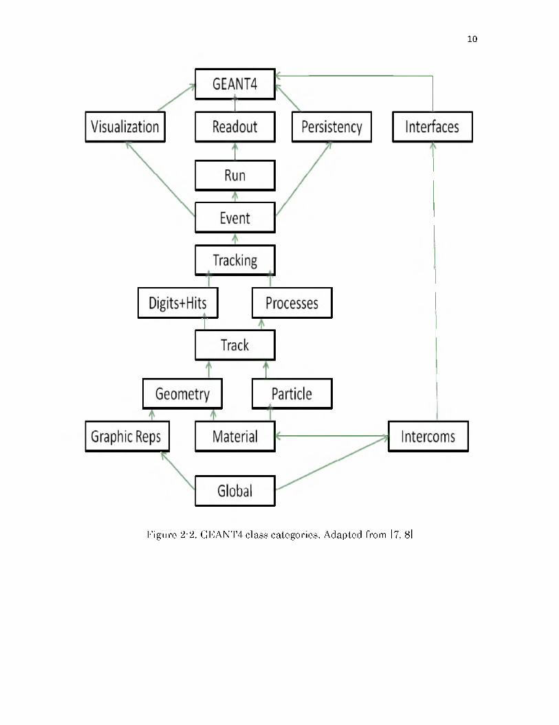
2.1.3. GEANT4 Functionality
The GEANT4 class categories are shown in Figure 2-2, and explained as follows
• Global category covers the system of units, constants, numerics, and random
number handling.
• M aterialsand particlescategories are implemented to describe the physical
properties of particles and materials for the simulation of particle
interactions.
• Geometry module is used to describe a geometrical model and propagate
particles.
• There are also categories required for describing the tracking of particles and
the physical processes they undergo. The track category contains classes for
tracking the particle interactions and steps, while the processes categories
contain implementations of models of physical interactions.
• Tracking category manages the evolution of a track’s state and provides
information in sensitive volumes for hits and digitization.
• Event category manages events in terms of the particle tracks, and the run
category manages collections of events that share a common beam and
detector implementation.
• Readout category allows the user to print the desired information.
9
10
Figure 2-2. GEANT4 class categories. Adapted from [7, 8]

11
• Finally, capabilities that use all of these categories and connect them
together within the GEANT4 code through abstract interfaces by providing
visualization, persistency, and user interface capabilities [1, 7, 8].
2.1.4. GEANT4 Benchmark and Accuracy
Electromagnetic processes can easily be described using theoretical methods
for very low to high energies. The precision of simulations most often depends on a
choice of implementation methods; therefore, validation of simulation codes depends
on direct comparison between simulation results, theoretical predictions, and
experimental work. At lower energies below 1 MeV generally, the analytical theory
tends not to be inaccurate [13], because it is necessary to describe the wave function
of atomic electrons in media. Cross-sections, stopping powers, and other physical
data are provided in evaluated data libraries. Simulation of electromagnetic
processes as well as other physics processes depends on tracking methods of the
particle that the user selects. The user can also specify the cut of energy of the
particle and the particle track path. Hence, the precision of most simulation codes
depends on chosen theoretical and physics models, parameterization methods, and
tracking parameters that are implemented by the user.
Regular regression tests and benchmarks are performed for all the physics
models implemented in GEANT4 [7, 8, 13]. Before the release of any GEANT4
package, the verification and validation of the electromagnetic (EM) physics models
are benchmarked and tested against known accurate data by the GEANT4 system
testing team [14]. For example, A. Lechner developed a benchmark experiment for

12
GEANT4 on electron backscattering energy deposition in semi-infinite media using
Sandia data. The electron energy of 0.1 - 1 MeV was evaluated and beam angles
were from 0 and 75 degrees, and GEANT4 results showed good accuracy with
existing data [15, 16]. Benchmarking of electromagnetic interactions was performed
at ATLAS using a barrel simplified calorimeter, and results showed no change of
energy of resolution [15, 16]. Validation and improvements of the GEANT4 standard
electromagnetic package at low energies performed by Vladimir Grichine, by
propagating particles through different target materials (Al, Au, Cu, and Si), showed
that the standard models have good agreement with the experiment (dE/dX) for
electron energy interval 0.01 - 10 MeV, and GEANT4 models for Bremsstahlung
benchmarked against experimental data also showed good agreement [17, 18]. Due
to the fact that GEANT4 is an open source code that has undergone many
generations of modifications pertaining to electromagnetic processes leading to the
release of different versions, not many benchmark experiments have been conducted
to compare some released versions of GEANT4. In Chapter 3, the benchmark of
different versions of GEANT4 codes used to model photon interactions are evaluated
against experimental data and MCNP5 modeling.
2.2. MCNP5 Code
The Monte Carlo N-Particle (MCNP) code is currently being managed by the
Diagnostic Application Group (Group X-5) in the Applied Physics Division (X
Division) at the Los Alamos National Laboratory [19]. MCNP is a general purpose
code that can be used to simulate neutron, photon, and electron transport. It is

13
capable of modeling complex 3D geometries and utilizes extensive point-wise cross
section data libraries in a continuous energy spectrum. It is applicable to modeling
nuclear interactions in medical physics, boron neutron capture therapy (BNCT),
high energy physics, radiation detection and shielding, particle accelerator models,
space study analysis, nuclear reactor simulations, and criticality calculations [19].
2.2.1. Applications of MCNP5
MCNP5 code is a Monte Carlo-based simulation of particle transport and
interactions with matter. MCNP5 is mostly used by nuclear engineers and scientist
around the world for a vast number of research simulations. MCNP5 has a wide
range of applications in the fields of medical physics, reactor physics calculations,
reactor safety calculations, and radiation dose estimates, as shown in Figure 2-3,
[20].
Reactor Physics Calculations Medical Physics
R adiation Dose R eactor SafetyInteractions A n alysis
Figure 2-3. Applications of MCNP. Adapted from [2]

14
2.2.2. MCNP5 Physics Processes
The very essence of MCNP is based on the probability of a physics interaction
of a neutron, photon, or electron. The MCNP is associated with having complete
accurate nuclear and atomic data libraries [19]. Data libraries provided in MCNP
contain information relating to the probability of unique particle interactions per
elements used during simulation. MCNP includes nine classes of data tables [20]: (1)
Continuous-energy neutron interaction data; (2) Discrete reaction neutron
interaction data; (3) Continuous-energy photoatomic interaction data;
(4) continuous-energy photonuclear interaction data; (5) neutron dosimetry
cross-sections; (6) neutron S(a,B) thermal data; (7) multigroup neutron, coupled
neutron/photon, and charged particles masquerading as neutrons; (8) multigroup
photon; and (9) electron interaction data. Physics interactions implemented in the
MCNP code for simulations include particle weight calculation, particle tracking,
neutron interactions, photon interactions, electron interactions, electromagnetic
interactions, and many more. During neutron interactions, a particle may collide
with a nucleus and will either be absorbed or scattered. Photon interactions include
coherent scattering and account for fluorescent photons after photoelectric
absorption, the Compton scattering from free electrons, photonuclear interactions,
and pair production. The transport of electrons and other charged particles is
fundamentally different from that of neutrons and photons. The interaction of
neutral particles is characterized by relatively infrequent isolated collisions, with
simple free flight between collisions. In contrast, the transport of electrons is

dominated by the Coulomb force, resulting in large numbers of small interactions,
Bremsstahlung, Cerenkov radiations, and other nuclear reactions [19, 20, 21].
2.2.3. MCNP5 Functionality
The MCNP5 input file contains five main categories as illustrated in Figure 2-4,
namely [2]:
• Geometry category- In order to describe the geometry of a model, one has to
specify the cell and the surfaces that make up the model. The material
composition of the cell is also specified in the geometry category.
• Source ca tegory-User specifies types of reactions and source(s) to be
simulated; for example, whether a source is a neutron source, or gamma
source. The user has the option to specify the energy or activity of the source
and the direction at which the source emits particles.
• Material card category-User chooses the elemental compositions that make
up the specified material in the geometry category and the data libraries
associated with the elements.
• Run mode category-This category determines a type of simulation being
performed; for example, either criticality calculation or particle interaction.
In addition, the run category gives a user an option to specify nuclear
reactions desired for the simulation as well as production of secondary
particles.
15

16
Figure 2-4. MCNP5 categories. Adapted from [2]
Tallies category - Provides summary information to a user related to particle
interactions, collision, creation and loss of particles, energy of particles,
radiation dose, particle flux, and much other useful information needed for
problem analysis.
2.2.4. MCNP5 Benchmark and Accuracy
Benchmarking of MCNP5 simulation codes against existing data for
verification and validation is very important due to the wide range of different
physics models, different code options, and different data libraries implemented
within the code. The verification of the simulation code is normally performed by

developers, and it involves performing a series of calculations to determine whether
a code solves the equations, computational models, and physical models it was
designed to solve [21, 22]. Validation of the MCNP5 simulation code is normally
performed by the end-users, and it involves the determination of whether the code
reproduces the true values of the simulated experiment or research or application.
Verification and validation also includes the comparison of the simulated results to
other codes, to analytical benchmarks, or to experiments [22].
MCNP5 developers have verified that MCNP5 produces accurate and the
same results as previous versions such as MCNP4 for a set of over a hundred test
experiments. For example, MCNP5 develops performed benchmarking of criticality
calculations by comparing MCNP5 simulations to previous versions of MCNP4 and
existing criticality data, and MCNP5 simulations showed good accuracy of criticality
calculations [22]. In addition, Y. Danon developed a benchmark experiment of
neutron resonance scattering models using MCNP. Experimental measurements of
elastic neutron scattering from U-238 resonances were used to benchmark neutron
scattering models in Monte Carlo transport codes. He found that MCNP5 elastic free
gas models have been improved to provide accurate simulation of the experimental
results [23]. Hanna Koivunoro performed simulations pertaining to the accuracy of
the electron transport in MCNP5 and its suitability for ionization chamber response
simulations [24]. She reported that the electron beam studies had some
discrepancies (>3%) at electron beam energies of 0.1 and 0.05 MeV. She also
concluded that MCNP5 provides dose distributions that agree better with other
17

reference codes, and MCNP5 results are highly dependent on the chosen electron
track length.
2.3. Summary of GEANT4 and MCNP5 Similarities and Differences
GEANT4 and MCNP5 are two simulation codes with similar features
embedded within the heart of the codes, yet different in their own unique aspects.
One of the most common features implemented in both codes are the Monte Carlo
methods. Monte Carlo methods are statistical principles that employ a class of
computational algorithms that rely on repeated random sampling to solve problems
that are of a probabilistic nature: for example, the interaction of nuclear particles
with materials. The Monte Carlo methods are also used to solve complex problems
that cannot be modeled with computational deterministic methods [2, 19]. Both
GEANT4 and MCNP5 codes are developed to be easily run along a wide range of
computer operation system platforms, such as Linux (GCC (g++)), and Mac OS X
(GCC (g++), Xcode 3 or 4) [1, 20]. Both codes are used for a wide range of research
applications, such as, but not limited to, high energy physics, medical sciences, space
radiation, nuclear engineering, and radiation science.
GEANT4 and MCNP5 have distinctive differences, including, but not limited
to, the following: (1) MCNP5 is developed by the Los Alamos National Laboratory
requiring individual licenses, while GEANT4, developed at CERN, is an open source.
(2) GEANT4 has several affiliated visualization codes such as OpenGL,
OpenInventor visualization, and X11 RayTracer [7, 8], while MCNP has its own
inbuilt visualization tool, VISED [20]. (3) MCNP5 requires INPUT file, whereas
18

19
GEANT4 is versatile and gives a user ability to program/code a desired geometry
and material definition, physics models, nuclear interactions, and output results. (4)
MCNP5 implements comprehensive physics models which include all nuclear
interactions processes possible, but GEANT4 has three different physics model
packages implemented within the code, namely, the Livermore physics model,
Standard physics model, and Penelope physics model [7, 15]. (5) One major
difference between MCNP5 and GEANT4 is the implementation of nuclear data
libraries used by both simulations codes; MCNP5 uses the Evaluated Nuclear Data
Files ENDF/B-VI [2] which are updated frequently, whereas GEANT4 implements
some data libraries extracted from the ENDF/B-VI and also, most of the data
libraries implemented are the EPDL97, EEDL, and EADL [16, 21].

CHAPTER 3
EXPERIMENTAL ASSESSMENT OF DIFFERENT GEANT4
CODE VERSIONS AND COMPARISON TO MCNP5
3.1. Description of Experiment to Benchmark GEANT4 and MCNP5
In order to benchmark versions of GEANT4 to determine which version
provides accurate simulation relative to photon transport and interaction, a photon
interaction experiment was conducted to benchmark experimental data with
simulation of different versions of GEANT4 and MCNP5 code using a cesium-137
source (137Cs). Cesium-137 has a half-life of 30.08 years, and specific activity of 3.214
TBq/g. The decay scheme of 137Cs is shown in Figure 3-1. Cesium-137 decays via beta
decay mode into a daughter nucleus of Barium-137 (137Ba) with maximum beta
energies of 0.512 MeV (94.6% probability) and 1.174 MeV (5.4% probability), and
emits gamma rays with energy of 0.6617 MeV during the transition from a meta-
Figure 3-1. 137Cs decay scheme. Adapted from [25]

stable to the ground state of 137Ba (Figure 3-1). Cesium-137 is used for a wide variety
of applications, both in the medical and industrial field, and not limited to treatment
of cancer, measurement of fluid flow in oil pipelines, well logging, and many more.
The Cesium- 137 gamma source was placed in the hollow cylindrical lead shielding
to minimize any unnecessary radiation dose to the researchers since the source is
very radioactive, and then placed on the open floor of the Nuclear Engineering
Facility, as shown in Figure 3-2. The gamma dose rates were measured at various
distances around the cesium- 137 source by placing a Ludlum model 19 potable NaI
detector at one foot intervals up to a distance of 8 ft around the set-up, as shown in
Figure 3-3. The Ludlum model 19 detector is a photomultiplier coupled to a 1” x 1”
NaI(TI) crystal, mounted inside the instrument housing. The detector is constructed
as a cast and aluminium cover with computer-beige powdercoating finish and
printed membrane front panel. The experimental measurement was repeated at
least five times to account for experimental error. The research was to simulate the
experimental set-up shown in Figures 3-2 and 3-3, using different versions of
Geant4. Benchmarking the experimental results with the Geant4 simulated results
to ascertain which version of Geant4 provides more accurate simulations pertaining
to photon transport, since the different versions of Geant4 have differences in their
physics models. Validation of the results was done with MCNP5.
21

22
Figure 3-2. Diagram of cesium source in Pig shielding (Not to scale)

23
Figure 3-3. Block diagram of the experimental set-up at UNEP facility (MEB 1205)(Not to scale)
3.2. Modeling of Gamma Interactions in GEANT4 and MCNP5
Different versions of GEANT4 (versions 4.9.2, 4.9.3, and 4.9.4) and MCNP5
codes (Appendix A and B) were used to simulate the experimental set-up in Figure
3-2 and Figure 3-3. The simulated data were compared and benchmarked against
obtained experimental data.
3.2.1. Modeling of Gamma Interactions in GEANT4
Versions of GEANT4.9.2, 4.9.3, and 4.9.4 have similar electromagnetic
models implemented within the code, but have unique different features. GEANT4

24
version 4.9.2 has three different independent electromagnetic physics package
models implemented within the heart of the code, namely, the Standard EM
package, Livermore EM package, and Penelope EM package. Each of the models has
different processes for describing photon interactions; for example,
G4PhotoElectricEffect (from the Standard EM package), G4LowEnergyPhotoElectric
(Livermore package) and G4PenelopePhotoElectric (Low Energy Penelope package)
[14].
GEANT4 version 4.9.3 is an improvement of GEANT4 version 4.9.2 that has
a few changes in its physics model. The low energy EM process in GEANT4.9.3 had
been migrated to follow the same software interface that was developed for the
Standard EM package. As a result, in the new approach, there is only one process
(e.g. G4PhotoElectricEffec£) and multiple independent models that can be registered
to the process, in different energy ranges, e.g. G4PEEffectModel (Standard),
G4LivermorePho-toElectricModel (LIVERMORE), and G4PenelopePhoto-
ElectricM odel(PENELOPE). New versions of two data sets were added : a low-
energy data set, G4EMLOW.6.9, and a new data set for optical surface reflectance
[26].
GEANT4 version 4.9.4 was developed to improve/address some shortcomings
of GEANT4.9.3. Geant4.9.4 includes modeling of pair production in the electric field
of secondary particles. The Bertini Cascade (BERT) model implemented in
GEANT4.9.3 was rewritten for Geant4.9.4 to improve memory management, and to
provide better energy/momentum conservation. Alongside, there was the addition of
a new physics list for BERT and CHIPS for shielding, and improved inelastic cross

sections at high energies. Also, eight new cross-section data sets for nuclear
interactions at low-energies were added to this package. Extensive validation of
physics models, which is fundamental to guarantee the accuracy and reliability of
Geant4-based simulations, has been documented by G.A.P. Cirrone et al. 2010 [14].
Photon interactions processes considered are as follows' The total cross
sections as a function of energy are derived from the evaluated data for all the
processes considered. For each process, the total cross-section at a given energy E is
obtained by interpolating the available data, according to the equation [10]'
log(<y(E)) = log(cr, ) log( ) + log(cr, ) ' ° i f ) -log(f . ) (3. i)SV ' " SV log(£2) - lo g fe ) S' - ' l o g f e ) - log(£,)
where E1 and E2 are the closest lower and higher energy for which cross-section 01
and 02 are available in the data libraries. In the photoelectric effect, the incident
photon is absorbed and an electron of direction identical to the one of the incident
photon is emitted. The subshell from which the electron is emitted is selected
according to the cross-sections of the subshell. The interaction leaves the atom in an
excited state, with excitation energy equal to the binding energy of the subshell from
which the electron has been emitted. The de-excitation of the atom proceeds via the
emission of fluorescence photons. The transition probabilities from a subshell to
lower energies are extracted from the EADL data library [26]. The fluorescence
photons are generated with energy determined by the energy difference of the
subshells involved in the transition and with isotropical distribution [10]. The
Livermore and Penelope cross-sections are tabulated according to EPDL97 and
EPDL89, respectively, and they are both in agreement with the NIST data cross-
25

26
section; however, the Standard model with respect to NIST data has a 10% deviation
[14]. During Compton scattering, the scattered photon energy is distributed
according to the product of the Klein-Nishina formula [10]:
<j(k) = 2m2 Z { k 2 - 2k - 2 "
2k 3ln(2K + 1) + k 3 + 9k2 + 8k + 2
4k4 + 4k3 + k 2(3.2)
where: ris classical electron radius, k = k/mc2
<P(e) = 1— + G G
1 - g sin'1+G2
(3.3)
photon scattering functions F (q ):
P(G q) = $(G)- F (q) (3.4)
where g is the ratio between the scattered photon energy and the incident photon
energy. The scattering functions F(q) at the transferred momentum q = E • sin2 (6 / 2)
corresponding to the energy E are calculated from the values available in the
EPDL97 data library. The angular distribution of the scattered photons is obtained
from the same procedure. The cross-section of the Standard package model
(G4KleinNishinaCompton) is derived from an empirical parameterized approach,
whose accuracy is estimated to be 10% between 10 and 20 keV, and 5-6% above 20
keV. The cross-section of the Geant4 Livermore model is tabulated according to the
EPDL97 library. The Penelope model is determined from an analytical
parameterization that takes into account atomic binding effects and Doppler
broadening for energies below 5 MeV, and uses the Klein-Nishina formula for energy
above 5 MeV [10, 14]. In the Rayleigh effect, the angular distribution of the
scattered photon is described by

^(E,0)=[l + cos2 O F 2 {q) (3.5)
where q = E ■ sin2 (0/2) is the transferred momentum corresponding to energy E and
F(q) i s the form factor. Form factors are obtained from the EPDL97 data libraries;
their dependence on the momentum transfer is taken into account by interpolating
the available data. The Standard EM package of Geant4 does not contain its own
model to describe Rayleigh scattering; only Livermore and Penelope models describe
Rayleigh scattering in Geant4. The cross-section of the G4LivermoreRayleighModel
is based on the EPDL97 database, while the cross-section of the Penelope model is
determined by numerical integration from an analytical parameterization [10, 14].
3.2.2. Modeling of Gamma Interactions in MCNP5
MCNP5 simulation code (Appendix A) was used to model the photon
interaction experiment depicted in Figure 3-3. There are two photon interaction
models implemented in MCNP' the Simple and Detailed model. The Simple photon
interaction physics model ignores coherent scattering and fluorescent photons from
photoelectric adsorption, and it is mostly used for high-energy photon problems [2].
The Detailed photon interaction physics model includes coherent scattering and
accounts for fluorescent photons after photoelectric absorption, and form factors as
well as Compton process are used to account for electron binding effects [2].
The photon interactions considered in MCNP are [2]' the total cross-section
calculation does not use the Klein-Nishina differential cross-section calculations.
Thus, the total cross-section o is regarded as the sum of three components' the
photoelectric cross-section-oe, Compton scattering-os, and pair production-Opp.
27

28
(3.6)
• Photoelectric effect- The incident photon is absorbed and an electron of
direction identical to the one of the incident photon is emitted, and treated as
a pure absorption by implicit capture with corresponding reduction in the
photon weight WGT, and hence does not result in the loss of the particle
history.
• Compton scattering-' in the interaction process of Compton scattering, the
physics is to determine the energy E ’of the scattered photon, and = cosd for
the angle dof the deflection from the line of flight. This yields the energy
WGT (E - E’) deposited at the point of collision and the new direction of the
scattered photon. The differential cross-section for the process is given by the
Klein-Nishina formula
where rois the classical electron radius 2.817938 x 10⁻¹³ cm, a and a'are the
m is the mass of the electron and c is the speed of light, and a ’ = a/(l+a(1-/i)).
• Pair production- in pair production, an electron-positron pair is created for
further transport and the photon disappears, or it is assumed that the kinetic
energy of the electron positron pair produced is deposited as thermal energy
at the time and point of collision, with isotropic production of one photon of
energy 0.511 MeV in one direction and another photon of the same energy in
the opposite direction.
j r / \ T 2 ^ ^ ^ 2 l 7K (a, fj)a^ = rno — -----1— r M ~ 1 dyy a ) ^a a \
(3.7)
incident and final photon energies in units of 0.511 MeV (a = E/(mc2), where

3.3. Experiment Assessment of Gamma Interactions Modeling using GEANT4 and MCNP5
The background dose rate at UNEP facility room MEB 1205 were measured
at various distances around the experimental area before the experimental set-up
was performed (Table 3-1) using the NaI detector. The NaI detector has a linearity
reading within ± 10% of true value. The NaI detector has a two-scale meter face
presenting 0-50 ^R/hr with full-scale range positions of 5000, 500, 50, and 0-25
^R/hr with full-scale range of 250 and 25. The measured gamma dose obtained from
the Ludlum model 19 potable NaI detector was recorded in mR/hr and converted to
mrem/hr with a conversion of 1 Roentgen (R) equal to 0.87 rems in dry air and 0.96
rems in tissue. Roentgen (R) is a measure of exposure to gamma ray or x-ray
radiation. One Roentgen is the amount of gamma radiation that will deposit enough
energy to strip about two billion electrons from their orbits in one cubic centimeter
of dry air. Rem is based on the biological damage casued by ionization in human
body tissue. The rem is also a term for dose equivalence and equals the biological
damage that would be caused by one rad of dose. Experimental data obtained were
benchmarked against versions of GEANT4 simulation and MCNP5. The dose
measurements were performed three times at each measured distance and the
average gamma dose, standard deviation, and standard error at each distance was
calculated.
29

30
Table 3-1. Background dose rate at various distances around experimental area
Distance(ft)
Time(min)
Average Background (mrem/hr)
1 0:30 0.00352 1:00 0.00353 1:30 0.00354 2:00 0.00355 2:30 0.00356 3:00 0.00357 3:30 0.00358 4:00 0.0035
The gamma dose rate can be calculated by either using the dose tallies in the
MCNP code or analytically by using the dose equations:
Gy C N Tsource) N j=1 i=1
T ^ t(E)H(E)
fwhere C = 1.602xlQ -10 Gy V
MeV/g1.10 -24 cm2 Y Na
Mbarn
Na = Avagadro’s constant = 6.022x10²³ mol-1;
q = number of atoms per molecule;
M = molar mass of material in grams;
(p= fluence score in particles/cm2;
ot = total atomic cross-section at energy of scoring track in barns;
H = heating number in MeV per collision at energy of scoring track;
N = number of source particles; and
T = number of scoring source particle tracks.
(3.8)
(3.9)

31
The equivalent dose could also be calculated depending on the energy deposited
within the target tissue based on the equation:
_13 T /
■ Energ ,Deposited , 1^ ? , L602jdr /MeV , g (310)mass 1
where g = ^ ^ (1 - e~M) (3.11)M
The average gamma dose rate can be expressed as:
N
n =
N
N n ? ?=1 (3.12)
N
where n is the average dose rate at each distance, n is the dose rate, and N i s the
number of dose rate measured. The standard error equation is expressed as:
E ( ’ <. _ n f' = N ( n _ 1 ) (3.13)
The two main photon interactions considered during simulation were
photoelectric effect and Compton scattering because the energy of emitted photon
particles from the cesium-137 source was 0.6617 MeV. Different versions of the
Geant4 codes were used to simulate the experimental set-up and simulations
presented in Table 3-2. The results obtained from the simulations of different
versions of Geant4 were benchmarked against MCNP5 simulation code and data
obtained in experiments. Gamma dose rate measured one foot away from the cesium
source was very high and decreased with an increase in measured distance away
from the cesium source. As expected, the gamma dose rate decreased as the distance
increased from the lead shielding. The trend of graphs obtained in Figures 3-4 and
32
3-5 follow the gamma exponential attenuation law. The slight differences in
simulation of GEANT4 versions and MCNP simulation was due to the different data
libraries implemented in codes. Even though the GEANT4 versions had different
physics models implemented for photon interactions, the simulations of GEANT4
versions presented good agreement with experimental data and MCNP5 simulation,
as indicated in Figure 3-4 and 3-5. Statistical analysis of error propagation with both
GEANT4 and MCNP5 simulation indicates good accuracy with dose rate measured
close to the source as compared to a further distance away from the detector; this is
due to particle angular dispersion as the particle traverses distance away from the
source (Table 3-2). The percentage difference between experimental results in
comparison to GEANT4 and MCNP5 is presented in Table 3-3, indicating marginal
differences between experimental results and simulations.
To calculate the percentage difference is given as: Percentage difference (Pd
%) = (1- (Simulated results/ experimental results)). For example, the percentage
difference between experimental results and MCNP5 at a distance of one feet (1 ft)
could be calculated as, Pd % = (1 - (27 / 27.667)) = 0.0241.

33
30.000
25.000
E0120.000
15.000
oQra 10.000 E
5 5.000
0.000
v\
\\ ............GEANT4.9.4
■ft GEANT4.9.3 ----------GEANT4,9,2
4 5Distance - feet
figure 3-4. Comparison of GEANT4.9.2, GEANT4.9.3, and GEANT4.9.4 gamma dose rate as a function of distance from the source
30.000
25.000
E<u20.000
o□tuEE1U
15.000
10.000
5.000
0.000
Distance - feet
Figure 3-5. Comparison of gamma dose rate as a function of distance from the source between the measured and calculated values using GEANT4 and MCNP5

34
Table 3-2. GEANT4 and MCNP5 dose rate in comparison to experimentalmeasurements
Distance — feet
Experiment — mrem/hr
MCNP5 - mrem/hr
GEANT4.9.4 - mrem/hr
GEANT4.9.3mrem/hr
GEANT4.9.2 - mrem/hr
1 27.667 ± 0.026 27.000 ± 0.051 26.843 ± 0.053 25.913 ± 0.063 24.500 ± 0.057
2 10.170 ± 0.089 10.000 ± 0.083 9.680 ± 0.084 9.200 ± 0.089 9.010 ± 0.085
3 3.830 ± 0.041 3.760 ± 0.087 3.712 ± 0.083 3.110 ± 0.093 3.001 ± 0.091
4 2.830 ± 0.128 2.810± 0.092 2.560 ± 0.101 2.240 ± 0.121 2.030 ± 0.113
5 1.420 ± 0.013 1.400 ± 0.094 1.348 ± 0.120 1.018 ± 0.133 0.990 ± 0.127
6 1.020 ± 0.013 1.000 ± 0.101 0.999 ± 0.123 0.960 ± 0.142 0.910 ± 0.131
7 0.920 ± 0.014 0.900 ± 0.137 0.870 ± 0.130 0.830 ± 0.150 0.789 ± 0.138
8 0.670 ± 0.015 0.700 ±0.142 0.580 ± 0.148 0.498 ± 0.153 0.401 ± 0.142
Table 3-3. Percentage difference between experimental measurements with GEANT4 and MCNP5 simulations
Distance - feet MCNP5 (%) Geant4.9.4 (%) Geant4.9.3 (%) Geant4.9.2 (%)
1 0.0241 0.02978 0.0634 0.1145
2 0.0167 0.04818 0.0954 0.1141
3 0.0183 0.03081 0.1880 0.2164
4 0.0071 0.09541 0.2085 0.2827
5 0.0141 0.05070 0.2831 0.3028
6 0.0196 0.02098 0.0588 0.1078
7 0.0217 0.05435 0.0978 0.1424
8 0.0448 0.13433 0.2567 0.4015

CHAPTER 4
BASICS ON FAST NEUTRON PENCIL BEAM FACILITY
4.1. About Fast Neutrons
In 1932, James Chadwick discovered the neutron particle. He performed
series of experiments at the University of Cambridge showing that the gamma ray
hypothesis was illogical and concluded that the new radiation consisted of
uncharged particles of approximately the mass of the proton. James Chadwick called
these uncharged particles neutrons [27]. James Chadwick’s discovery proved that
there is a neutral particle in the nucleus and that there are no free electrons in the
nucleus, as postulated by Ernest Rutherford. The neutron is a subatomic hadron
particle, which has no electric charge, and therefore does not cause direct ionization
of matter. Neutrons are found within the atomic nucleus as they bind with protons
via the nuclear force. Neutrons do not interact with electrons but interact with the
nucleus. The number of neutrons in a nucleus determines the isotope of an element
[28]. Free neutrons decay with a half-life of about 10.3 min [28]. There are two types
of neutron interactions: Compound Interactions - the neutron as a projectile
interacts with a target nucleus, forming a compound nucleus (half-life ~10-16 sec) and
decays in different channels and has no memory of its formation; and Direct
Interactions - an incoming neutron interacts with the nucleus but does not disturb
other nucleons within the target nucleus; thus, the time for a neutron as a projectile
particle to traverse a target nucleus is ~ 10 ■22 sec [27, 28].
36
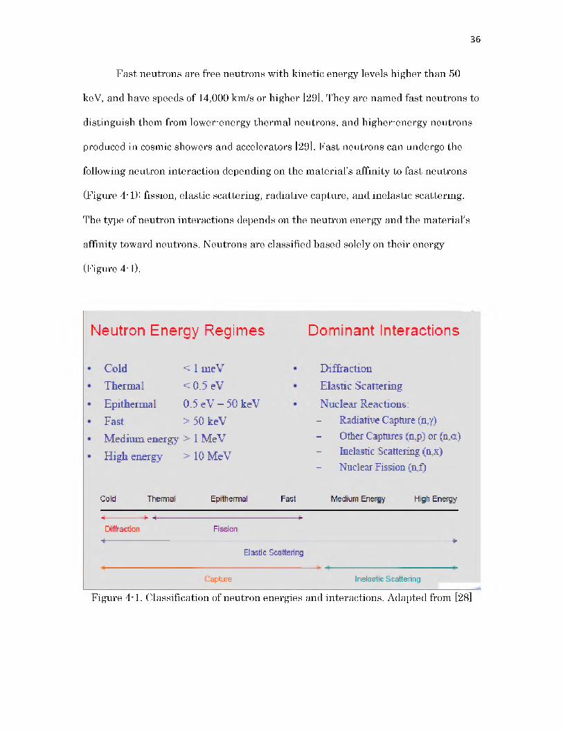
Fast neutrons are free neutrons with kinetic energy levels higher than 50
keV, and have speeds of 14,000 km/s or higher [29]. They are named fast neutrons to
distinguish them from lower-energy thermal neutrons, and higher-energy neutrons
produced in cosmic showers and accelerators [29]. Fast neutrons can undergo the
following neutron interaction depending on the material’s affinity to fast neutrons
(Figure 4-1): fission, elastic scattering, radiative capture, and inelastic scattering.
The type of neutron interactions depends on the neutron energy and the material’s
affinity toward neutrons. Neutrons are classified based solely on their energy
(Figure 4-1).
Neutron Energy Regimes Dominant Interactions
Cold
Thermal
Epithermal
Fast
< 1 meV<0.5 eV 0.5 eV - 50 keV > 50 keV
Medium energy > I MeV High energy >10 MeV
Diffraction
Elastic Scattering
Nuclear Reactions:
- Radiative Capture (n,y)
- Other Captures (nrp) or (a ,a )
- Inelastic Scattering (n;x)
- Nuclear Fissioa (n f)
Cold Thermal Epithermal Fast Medium Enenjy High Energy
Diffraction Fission
Elastic Scattering
liapture Inelastic Scattering
Figure 4-1. Classification of neutron energies and interactions. Adapted from [28]
37
Fast neutrons can be produced, found, or generated from a wide variety of
different neutron sources: from neutron accelerators, operating research reactors,
spallation neutron source, radioisotopes which decay with alpha particles packed in
a low-Z elemental matrix (e.g. Am-Be) [27], and isotopes that produce neutrons
spontaneously (e.g. 98CP52) [27]. The main sources of fast neutron production are by
nuclear fission, which produces fast neutrons with a mean energy of 2 MeV (200
TJ/kg, i.e. 20,000 km/s) [27, 29]; and by particle accelerator with the emission of a
proton particle to hit a tungsten, target producing fast neutrons with energies of
about 14.1 MeV (1400 TJ/kg, i.e. 52,000 km/s, 17.3% of the speed of light) [27, 29]
and can easily fission uranium-238 and other nonfissile actinides.
4.2. Fast Neutron Facilities
Fast neutron facilities can be classified based upon the neutron flux
produced, neutron energy, size and type of source, costs, government regulations,
and application. Fast neutron sources can be used for a wide diverse range of
applications. Most common applications of these neutron facilities are in the areas of
engineering, medicine, nuclear weapons, petroleum exploration, biology, chemistry,
nuclear power, applied nuclear physics, and other industries (Table 4-1). Fast
neutron facilities are located all around the world; to mention a few: The Institute of
Neutron Science Laboratory - Institute for Solid State Physics (University of Tokyo),
Oak Ridge Neutron Facilities (SNS/HFIR), Los Alamos Neutron Science Centre
(LANSCE), Bhabha Atomic Research Centre (Mumbai India), FRM-II Lab (Munich
Germany), Bragg Institute (ANSTO Australia), Braunschweig Accelerator Facility,
and many other facilities.

38
Table 4-1. Applications of fast neutron facilities [30]
General Area Specific ApplicationsGeophysical Science Mine mineral mapping and analysis
Petroleum exploration Quarry mineral mapping and analysis Uranium exploration Nuclear well logging
Industrial Cement processing Coal quality analysis Wall thickness analysis Metal fracture detection
Security Explosives detections and identificationChemical weapon agent detection and identificationSpecial nuclear materials detection and identificationLand mine detectionUnexploded ordnance inspectionFast neutron radiography
Medicinal Sciences Nuclear medicine Fast neutron therapy
Nuclear Engineering Fast breeder reactors Nuclear reactor analysisFast neutron reference source for instrumentation Calibration source for neutrino observatory instrumentation Studies of radiation damage to electronic component Spallation neutron source
Environment Nuclear waste assayWaste assay for resource conservation and recovery Carbon sequestration quantification in soil
4.2.1. Application of Fast Neutron Facilities
Fast neutron facilities are used in a myriad of applications, including neutron
therapy for the irradiation of cancer cells and tumors, neutron detection for the
detection of nuclear materials and neutron radiography, and industrial applications
for nuclear well logging, and detection of cracks in concrete and metals. Applications
of fast neutron facilities include, but are not limited to, the following:

• Fast neutron irradiation facility' there is vast number of fast neutron
irradiation facilities in the world used for a wide range of research. Most
institutes with research reactors have a fast neutron irradiation facility used
for a wide range of research. For example, The University of Utah Triga
reactor has a Fast Neutron Irradiation Facility (FNIF), mainly used for
research in the field of Neutron Activation Analysis (NAA). The University of
Massachusetts Lowell also has a fast neutron irradiation facility used for fast
neutron irradiation of samples for elemental analysis. Also, the fast neutron
facility at the ISIS Spallation neutron source is used for irradiation tests of
electronic components and the beam line has a neutron energy range above
10 MeV [31].
• Fast neutron detection facility' There are a couple of institutions that deal
with the detection of fast neutrons, which is a technique that could be used
for detection of nuclear materials. Most neutron detection techniques rely on
observing a neutron-induced nuclear reaction, but the captured cross-sections
for fast neutron-induced reactions tend to be small and hard to detect
compared to neutrons at lower energies. Two approaches are normally used
by detection facilities, namely, Thermalized and Capture (fast neutrons are
thermalized in order to detect) and Elastic scatter from protons at high
energy (observed recoils for TOF techniques) [32].
• Linear accelerator facilities' electron or proton beams produced in linear
accelerators can be used to efficiently produce fast neutrons by photonuclear
reactions. This process involves the acceleration of collimated electron or
39
proton beams at high velocity to hit a beryllium (Be) or tungsten target to
produce fast neutrons at high energies of about 14 MeV. Neutron accelerator
facilities have a broad range of research applications in the areas of
industrial, medical dosimetry, homeland security, radiation hardness testing,
and radiation effects on materials. An example of such a facility is the NIST
accelerator facility used for a number of research such as [33]' (a) broad-
energy range calibration of charged-particle spectrometers used in space
flight applications, (b) calibration of a beta spectrometer employed in a
fundamental nuclear physics measurement of the neutron lifetime, (c) solar
cell performance validation studies at several different electron energies and
fluencies, and (d) development of a variable-speed radiation scanning system.
• Fast neutron therapy facility- fast neutron facilities have been applied in the
medical sciences for the treatment of cancer, and plasma and beam physics
research for years. Clinical institutions began supporting clinical fast neutron
clinical studies in the world beginning in the early 1970s using physics-based
cyclotrons and linear accelerators at a number of facilities around the world.
The clinical treatment of cancers and tumors using fast neutrons is being
researched and continue to be modified due to advancement in technology by
accredited research institutions around the world. Some hospital-based
neutron facilities currently being operated in the United States are the
University of Washington in Seattle, University of California in Los Angeles,
the University of Texas System Cancer Center in Houston, and many other
institutions.
40

41
4.2.2. Application of Fast Neutron Pencil Beam Facilities
Fast Neutron Pencil Beam (FNPB) facilities around the world (Table 4-2) are
applied in a couple of fields; most common amongst the applications are for fast
neutron therapy for the cure of cancer and tumors and also for studying the
radiation effects on electronic component’s displacement damage and ionization. A
fast neutron pencil beam is produced using neutron reflective materials to collimate
fast neutrons to produce a thin fast neutron beam. The diameter of the fast neutron
beam is mostly between 2 cm to 3 cm. A variety of fast neutron facilities have been
used to study the response of electronics to displacement damage and ionization in
electronic components. The test model is important for the study of radiation
damage and hardness of electronic components associated with aircraft and space
exploration. A new test methodology using FNPB produced from a 6.5 MeV tandem
accelerator alongside high fidelity computational models has been used to study this
effect [36]. Fast neutron pencil beams are mostly produced using neutron generators
for Fast Neutron Therapy (FNT), such as cyclotron accelerators and reactors. The
FNPB uses the effects of high-LET (linear energy transfer) radiation (secondary
recoil protons and alpha particles, respectively) to attack/irradiate radio-resistant
tumors and cancers, considering hazardous effects for irradiated healthy tissue. In
research conducted by E. Bourhis-Martin at the University of Essen, Germany, the
fast neutron pencil beam for therapy is produced by a nuclear reaction of 14.3 MeV
deuterons emitted on a thick beryllium target (diameter of 30 mm and thickness of 5
mm) according to the nuclear reaction: 9Be+2H ^ 10B+m+Q with Q = 4.36 MeV, and
9Be+2H ^9Be+n+p+Q with Q = 2.2 MeV.

42
Table 4-2. Fast Neutron Therapy (FNT) facilities around the world [37]
Country,Location
References
SourceReaction
Approx.mean
n-Energy[MeV]
50-%-depth[an]
BeamDirection
Collimator FirstTreatment
PatientDumber
Status Mainindications
Treatmentplanningsystem
USBatavia,;1L Fermilab [4,5]
LINACp(66)+Be
25 IE horizontal Inserts 1976 3300+ active H&NInhouse,
modified M INUII
USSeattle:'VA Univ. of Washington CN IS [6-10]
Cyclotl'ond(50.5)+Be
20 14Isocentrichorizontal
MLC*Inserts
1984 28D0+ activeSalivaiy gland,
sarcomasPrism, now
modified Pinnacle
USDetroitMIHarper Hospital/WSU [11-13] '
Cyclotl'ond(48.B)+Be
20 13Isocentric,
IMRTMLC 1990 2140
active(refurbishme
nt)
Lung cancer, late prostate
VRSplan(modifiedGRATIS)
ZASomerset West [14-18]
Cyclotl'onp(66)+Be 25 16 Isocentric
Variable jaws + multiblade
trimmer1988 1685+ active
salivary gland, H&N, soft tissue,
sarcoma, osteosarcoma,
breast, malignant melanoma
VKTUOS (from DKFZ**)
RUTomsk Polytechnic University [19]
Cyclotl'ond(13.5)+Be
6.3 6 Horizontal Inserts 1984 1500+ activeH&N, salivary gland, breast
MCNP
RUSueztiiusk V N E IF [20-22]
D-T-Geneiator
10,5 S Horizontal Inserts 1999 990+ Standby Nose, throat, thyroid
SERAPRIZM
DEGarching/Mimich FRM I/FRM D [23, 24]
Fission of uranium
1.9 5.0 Horizontal Inserts MLC 198 5,'2007 820 active
Recurrent breast cancer,
malignant melanoma
SERA, MCNPX
The energy spectrum of fast neutrons has a mean and maximum energy of
5.5 and 18 MeV with a fast neutron flux within a range of ~106 to 108 n/cm2s,
respectively, for patient treatments [35]. Other neutron sources for FNT have been
cyclotrons, D-T neutron generators, and the accelerator at the FERMI-Lab. Earlier,
a fast reactor (BR-10 at Obninsk, Russia) and 252Cf have also been used with average
neutron energies from 2 MeV (fission neutrons) to about 25 MeV for cyclotrons [36].

According to research conducted by F. M. Wagner [37], FNT has been
administered to over 30,000 patients world-wide. From formerly 40 facilities around
the world, now only eight are operational. This is due to the technical and economic
conditions and also the side effects associated with damage of healthy tissue and
insufficient proof of clinical results in the early years. FNT is not recommended for
all cancers, but rather for predominantly adeno-cystic carcinoma (ACC) of salivary
glands, as this type of tumor is rare. FNT is also administered in palliative
situations where the tumor/cancer is recurrent or irresectable and for very extended
tumors [37]. One such facility is the Detroit FNT facility located at Harper Hospital,
Gershenson Radiation Oncology Center, Karmanos Cancer Institute, and Wayne
State University (KCC/WSU) in Detroit. The FNT is produced by a gantry-mounted
superconducting cyclotron, with a 120-leaf collimator that delivers more radiation
dose to the tumor [37]. Overall, FNT has its niche in routine medical treatment of
selected malign tumors and their recurrences [37].
43

CHAPTER 5
PRELIMINARY DESIGN OF THE FAST NEUTRON PENCIL
BEAM FACILITY AT THE UNIVERSITY
OF UTAH TRIGA (UUTR)
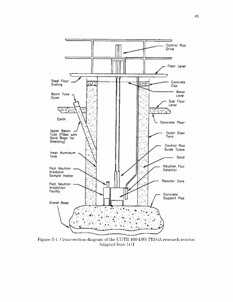
5.1. General Characteristics of the UUTR
The University of Utah TRIGA (Training, Research, Isotope, General
Atomics) is a pool-type research reactor that operates at 100 kilowatt thermal
power. The core of the reactor is a hexagonal lattice of an aluminum grid structure
submerged at the bottom of a deep tank filled with purified water, [38] as shown in
Figure 5-1. The TRIGA reactor is mostly used by educational and research
institutions for research, teaching, and training. The UUTR uses light water as
coolant and the cooling process is by natural convection circulated through a mixed-
resin bed ion-exchange system to maintain high purity of the water. The UUTR also
uses light water as a neutron moderator, and radiation shielding, in addition to
representing a heat sink [38]. The UUTR reactor core has a heterogeneous assembly
of standard fuel elements made of zirconium hydride mixed within the uranium
matrix, and deuterium oxide (D2O, “heavy water”) and graphite element as reflective
material. Both the heavy water and graphite elements surround the core and
moderate leakage neutrons from the reactor core and provide an isotropic thermal
neutron environment suited for neutron activation via (n, r) reaction. UUTR has
45
Figure 5-1. Cross-section diagram of the UUTR 100-kWt TRIGA research reactor.Adapted from [41]
46
three neutron-absorbing control rods (CR) containing boron carbide (B4C). The
UUTR has four neutron irradiation ports: a thermal neutron irradiation (IT) port,
fast neutron irradiation facility (FNIF), central neutron irradiation (CI) port, and
pneumatic neutron irradiation port.
5.2. Conceptual Design of the Fast Neutron Pencil Beam Facility at the UUTR
The goal of this research is to develop a preliminary study and a model of a
fast neutron pencil beam facility at the UUTR for various research applications. The
UUTR has only one fast neutron irradiation port (FNIF). This port is capable of
providing fast neutrons necessary for the fast neutron pencil beam facility. The
FNIF is composed of a heavy lead manufactured box, with a sample holder lid made
of aluminum [40]. Figure 5-2 shows a cross-sectional diagram of the FNIF showing
its vertical orientation relative to the reactor core [41]. The FNIF was purposely
designed to provide fast neutron irradiation with a quasi-fission energy spectrum
and low photon exposure, due to the heavy lead material shielding. Fuel elements
are adjacent to the FNIF in providing a planar fission neutron source with fast
neutron component being dominant. The FNIF is placed very close to the reactor
core to minimize the moderation of fast neutrons by the pool water (Figure 5-3). The
concept design of the FNPB facility is to optimize the design to provide enough space
for fast neutrons from the FNIF to be collimated through a thin tube of space. The
FNPB is designed as box with an air space that will be placed on top of the FNIF to
enable fast neutrons to flow from the air gap. The FNPB consists of three parts: an
aluminum casing, the FNPB box, and the sample holder, as shown in Figure 5-4.

47
Figure 5-2. Vertical cross-section diagram of FNIF. Adapted from [41]
Figure 5-3. Outline of UUTR reactor and FNIF

48
Figure 5-4. UUTR FNPB model
The aluminum casing is hollow with a one inch lead layer at the bottom to enable
it to sink beneath into the FNIF to block the air gap and prevent water from
entering, since the water will moderate the fast neutrons to thermal neutrons. The
FNPB box sits on top of the aluminum casing and the FNIF. The sample holder fits
inside the top of the FNPB box. Material composition normally considered for
collimation of fast neutrons should be a neutron reflector. When a neutron interacts

with matter, it is either absorbed or scattered. The materials should have the
tendency to scatter fast neutrons. To select the materials best suitable for neutron
scattering, the material cross-sections related to elastic scattering, absorption, and
secondary particle production are closely examined. The materials selected have
high affinity for elastic and inelastic scattering for fast neutrons. The resonance
peaks occur when there is intermediate formation of compound nucleus. Materials
considered for modeling the UUTR FNPB are: aluminum, boron10, paraffin, lead,
and graphite.
Aluminum: based on cross-sections, the aluminum does not have high absorption
nor a scattering cross-section for fast neutrons (Figure 5-5). Aluminum is a low-Z
element with density of 2.7 g/cm3. Pure aluminum has good material properties
with water due to its ability to resist corrosion; therefore, aluminum thickness of 0.5
cm is used to model the aluminum
49
i— i i i i ir i j------- 1— i r m 111 1 -------1— i i 1 1 i i i|------- 1— i i 1 1 1 i i j ------- 1— i rTTTTTj-------1— i n n r | -------i— i- r m r r | ------- 1— i i i m i | -------1— i i i r n i| ------- 1 r r r i u r j — !
10
10;V
10 ‘
aio1c.° O ^10° oUCOnio1 -<s> -© “ < io2 r 103 l~ 104 io'
Elastic scattering
Radiative capture Inelastic scattering =a/ -
J
.....................................i i i 1 1 m l_____I___i ..............I_____I___» i i m i l _____|___i i m i l l _____I__ i ..............I........... ......................... I.......... ......................... ............I I I 1 1 I I liL-J
Energy (MeV)
Figure 5-5. Cross-section plots of aluminum-Al. Adapted from [42]

casing to cover the FNIF air gap, and also to cover both the out layer of the
FNPB box and the sample holder box.
• Boron-10- boron (B-10) has density of 2.08 g/cm3, and has a high (n, a)
reaction and absorption cross-section for thermal neutrons in a (n, D)
reaction, but does not absorb fast neutrons, based on cross-section plots in
Figure 5-6. Boron (B-10) with thickness of 0.5 cm is used to line the inner
surface of the FNPB box to absorb thermalized fast neutrons within the pool
water that propagates through the aluminum covering. A thin layer of B-10,
of about 0.2 cm, is also placed at the window tip of the collimation tube to
absorb moderated neutrons to reduce a thermal neutron flux of pencil beam
entering the sample holder.
• Graphite' graphite is a good material used in most rectors to reflect leaked
neutrons back into the reactor core, and has a density of 1.7 g/cm3. Figure 5-7
indicates that the graphite is a good moderating material and has good
propensity to scatter neutrons. Graphite is one of the materials considered for
the collimation of fast neutron pencil beam based on its nuclear properties.
• Lead' lead is a very good shielding material for attenuating gamma rays, and
has poor affinity for neutrons, based on cross-section plots in Figure 5-8. Lead
is a very dense material with density of 11.354 g/cm3. An inch of lead is
modeled within the bottom of the aluminum casing to enable it to sink into
the reactor pool and FNIF. The inner layer of the sample holder is made of
0.5 cm of lead to attenuate gammas emitted from the top of the core to
prevent radiation damage to the sample, in case of a biological sample.
50

51
Figure 5-6. Cross-section plots of boron-(B-10). Adapted from [42]
Energy (MeV)
Figure 5-7. Cross-section plots of graphite-C. Adapted from [42]

52
io J --
10 -
i iiiiij—i 11iiuij—i 11iiiiij—i 11iiiiij—i 11 iiiiij—i 11 iinij—i 111uiij—i niiiiij—i 11iiiMj— i 11uiiij i
Pb
10 r-S lO 1
° Ol" +3-v ro = <b -1v> ol. -9 °1010v10410-5
Eldblic scdLLerinj=;
Radiative capture
1 I n i ml..... .......... Ill___i i i mill__ i i i mill__ l 11 11 ml__ l l l mill__ i i 11 mil__ i l ....... I__ l i m ini__ i i 111mil mil mil ml
Ine ldsL ic s c a lL j;r in g
mil ... I m ill m il '
109 10® 10' 100 6 105 104 103 102 101 1$ l i
Energy (MeV)
Figure 5-8. Cross-section plots of lead-Pb. Adapted from [42]
• Paraffin: paraffin is composed of 85.4% carbon and 14.6% hydrogen; its
chemical compound is C20H42 to C40H82. Hydrogen has no excited states,
therefore, it has no formation of a compound nucleus or resonances.
Hydrogen has good affinity to absorb thermal neutrons and has good
scattering ability for fast neutrons, as shown in Figure 5-9. Hydrogen mixed
with carbon to form paraffin provides good scattering of fast neutrons, and
could be used either as reflective material or for neutron shielding.
The following is the description of the preliminary design of the fast neutron
pencil beam facility at the UUTR:
• Aluminum casing- The aluminum casing is made of pure aluminum with an
inch thickness of lead molded to the bottom of the casing to enable it to sink

53
Energy (MeV)
Figure 5-9. Cross-section plots of Hydrogen-H. Adapted from [42]
deep into the reactor pool to cover the FNIF air gap and thus prevent water
from entering. The aluminum casing is about 0.5 cm thick, has a height of
55.88 cm, a length of 10.16 cm, and a width of 17 cm, and has two small
holding handles at the side for easy removal or placement within the pool, as
shown in Figure 5-10.
• FNPB sample holder- The FNPB sampler holder is designed to house any
sample to be irradiated via the fast neutron pencil beam. The sampler holder
is hollow, coated with pure aluminum, with a 0.5 cm inner layer of lead to
reduce gamma flux within sample holder. The sample holder is a box of 6 cm
height, 6 cm width, 5 cm in length, and has a polyethylene tube at the top for
easy placement and removal of samples. The sample holder fits on top of the
FNPB box, and has two small handles for easy placement and removal, as
shown in Figure 5-10.
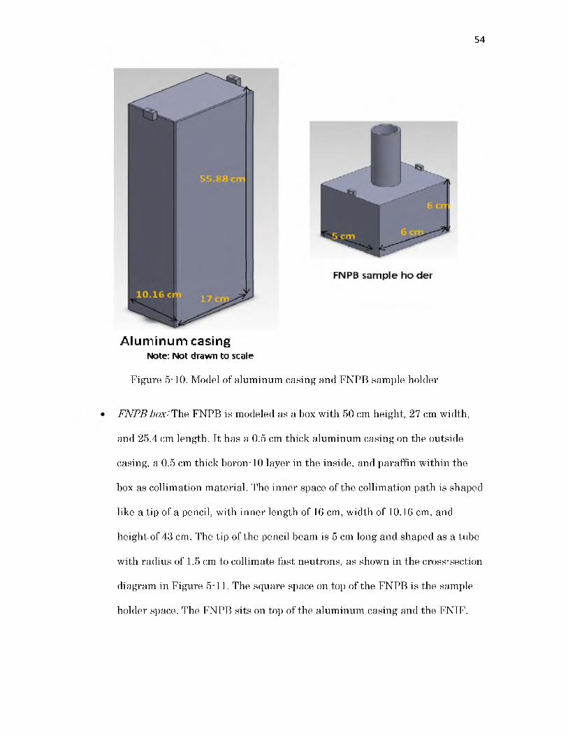
54
Aluminum casingNote: Not drawn to scale
Figure 5-10. Model of aluminum casing and FNPB sample holder
FNPB box: The FNPB is modeled as a box with 50 cm height, 27 cm width,
and 25.4 cm length. It has a 0.5 cm thick aluminum casing on the outside
casing, a 0.5 cm thick boron-10 layer in the inside, and paraffin within the
box as collimation material. The inner space of the collimation path is shaped
like a tip of a pencil, with inner length of 16 cm, width of 10.16 cm, and
height of 43 cm. The tip of the pencil beam is 5 cm long and shaped as a tube
with radius of 1.5 cm to collimate fast neutrons, as shown in the cross-section
diagram in Figure 5-11. The square space on top of the FNPB is the sample
holder space. The FNPB sits on top of the aluminum casing and the FNIF.

55
Figure 5-11. Cross-section model of UUTR FNPB
5.3. MCNP5 Model of the Fast Neutron Pencil Beam Facility at the UUTR
The UUTR FNPB was modeled using the MCNP5 following the design as
described. Figures 5-12 and 5-13 show the 3-D and the cross-sectional diagram of the
UUTR FNPB design, respectively. The MCNP5 FNPB facility model includes the
exact model of the UUTR reactor core, with all fuel specifications, moderator
material, reflector material, and control rods. The data libraries used for simulation
are ENDF-VII data libraries at temperature of 300 K. The source of fast neutron
was generated from fission simulation of reactor fuel within the reactor core.
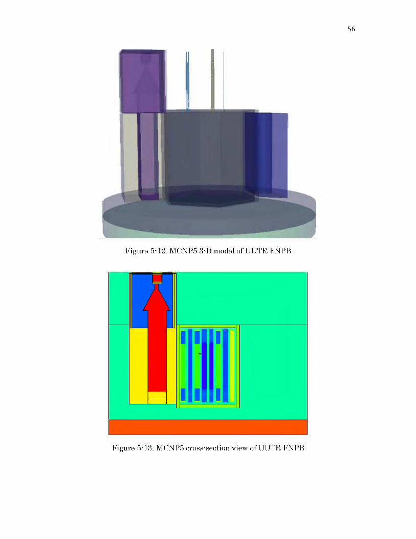
56
Figure 5-12. MCNP5 3-D model of UUTR FNPB
Figure 5-13. MCNP5 cross-section view of UUTR FNPB

5.4. GEANT4 Model of the Fast Neutron Pencil BeamFacility at the UUTR
The UUTR FNPB was modeled using GEANT4.9.4 simulation code (Appendix
F). The GEANT4.9.4 classes implemented are the following: G4DectorConstruction
class was implemented for the construction of the UUTR FNPB geometry, and
material specifications; G4PhysicsList was used to specify the physics interaction of
the neutron interactions with matter; the neutron source was implemented using
the G4GeneralParticleSource class, and modeled as a square planar source with a
Maxwellian energy spectrum placed at the side of FNIF, as shown in Figure 5-14;
and G4SteppingAction was used to get desired information needed from the
simulation, such as change in energy and direction of the particle printed as a text
document. Neutron data libraries implemented in GEANT4.9.4 used for the
simulation are some imported ENDF-VII MCNP data libraries and EPDL97 data
libraries.
5.5. Comparison of GEANT4 and MCNP5 in ModelingNeutron Interactions
Despite the fact that both GEANT4 and MCNP5 codes are based on Monte
Carlo methods, they are different in various aspects, as described in Chapter 2.
GEANT4 and MCNP5 (Appendix C and D) simulation of neutron interactions with
selected materials were assessed based on a simple model represented as a
rectangular cubic box with the following dimensions: length 4 cm, height 4 cm, and
width 2 cm.
57

58
3-D view of UUTR FNPB
Figure 5-14. GEANT4 model of UUTR FNPB
The neutron source was modeled as a disc surface source placed at the centre of one
side of the cube; the neutron source was assumed to be mono-energetic and two
different energies were considered- 0.025 eV and 2 MeV. Materials are selected
based on the basic materials as used in the preliminary design of FNPB at the
UUTR, i.e. lead, boron, and paraffin. Figures 5-15 to 5-17 show the GEANT4 and
MCNP5 resulting neutron interactions at different energies with boron-10, lead, and
paraffin. Table 5-1 summarizes a comparison of GEANT4 and MCNP5 results as
follows- for 10,000,000 neutron particles, the effect of interactions with selected
materials at two different neutron energies of 0.025 eV and 2 MeV, neutron and

59
Figure 5-15. GEANT4 and MCNP5 simulation of neutron interactions with boron-10
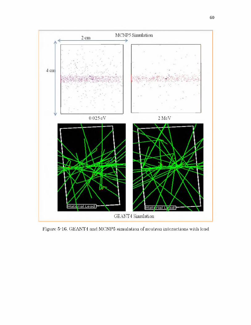
60
GEANT4 Simulation
Figure 5-16. GEANT4 and MCNP5 simulation of neutron interactions with lead
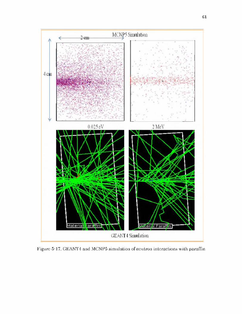
61
MCNP5 Simulation
GEANT4 Simulation
Figure 5-17. GEANT4 and MCNP5 simulation of neutron interactions with paraffin
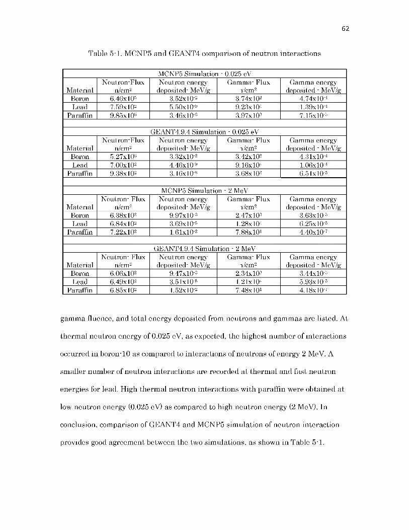
62
Table 5-1. MCNP5 and GEANT4 comparison of neutron interactions
MCNP5 Simulation - 0.025 eV
MaterialNeutron-Flux
n/cm2Neutron energy
deposited- MeV/gGamma- Flux
i/cm2Gamma energy
deposited - MeV/gBoron 6.46x10⁵ 3.52x10⁻² 3.74x10² 4.74x10⁻⁴Lead 7.59x10² 5.50x10⁻⁹ 9.23x10⁴ 1.39x10⁻⁴
Paraffin 9.85x10⁵ 3.46x10⁻⁶ 3.97x10³ 7.15x10⁻⁵
GEANT4.9.4 Simulation - 0.025 eV
MaterialNeutron-Flux
n/cm2Neutron energy
deposited- MeV/gGamma- Flux
i/cm2Gamma energy
deposited - MeV/gBoron 5.27x10⁵ 3.32x10⁻² 3.42x10² 4.31x10⁻⁴Lead 7.00x10² 4.46x10⁻⁹ 9 .16x104 1.06x10⁻⁴
Paraffin 9.38x10² 3.16x10⁻⁶ 3.68x10³ 6.51x10⁻⁵
MCNP5 Simulation - 2 MeV
MaterialNeutron- Flux
n/cm2Neutron energy
deposited- MeV/gGamma- Flux
i/cm2Gamma energy
deposited - MeV/gBoron 6.38x10² 9.97x10⁻³ 2.47x10³ 3.63x10⁻⁵Lead 6.84x10² 3.69x10⁻⁵ 1.28x10⁴ 6.25x10⁻⁵
Paraffin 7.22x10² 1.61x10⁻² 7.88x10! 4.40x10⁻⁷
GEANT4.9.4 Simulation - 2 MeV
MaterialNeutron- Flux
n/cm2Neutron energy
deposited- MeV/gGamma- Flux
i/cm2Gamma energy
deposited - MeV/gBoron 6.06x10² 9.47x10⁻³ 2.34x10³ 3.44x10⁻⁵Lead 6.49x10² 3.51x10⁻⁵ 1.21x10⁴ 5.93x10⁻⁵
Paraffin 6.85x10² 1.52x10⁻² 7.48x10! 4 .18x10-7
gamma fluence, and total energy deposited from neutrons and gammas are listed. At
thermal neutron energy of 0.025 eV, as expected, the highest number of interactions
occurred in boron-10 as compared to interactions of neutrons of energy 2 MeV. A
smaller number of neutron interactions are recorded at thermal and fast neutron
energies for lead. High thermal neutron interactions with paraffin were obtained at
low neutron energy (0.025 eV) as compared to high neutron energy (2 MeV). In
conclusion, comparison of GEANT4 and MCNP5 simulation of neutron interaction
provides good agreement between the two simulations, as shown in Table 5-1.

63
5.6. Comparison between MCNP5 and GEANT4.9.4 Models of the Fast Neutron Pencil Beam Facility at the UUTR
MCNP5 and GEANT4.9.4 were used to model and simulate the UUTR FNPB
design as described in previous sections. The MCNP5 input file (Appendix E) of the
UUTR FNPB simulated the reactor core from which the fast neutron source was
emitted from the fission process in the core. The reactor core was modeled at 90 kW
power with all control rods out. Table 5-2 shows a summary of MCNP5 simulation of
UUTR FNPB- the reactor remained critical with kefrof 1.0065 (with good standard
deviation and relative error of 0.00003 and 0.0275, respectively). The FNIF has an
estimated fast neutron flux of ~ 1011 n/cm2 s. The probability of fast neutron
scattering into the UUTR FNPB sample holder is on the order of 1-10,000 based on
the ration of neutrons recorded in the sample holder relative to the FNIF. The fast
neutron flux of the FNPB is 6.52x10⁷ n/cm2s delivering a neutron dose of 4.24x10⁴
rem/hr as shown in Table 5-2. The neutron spectrum, indicated in Figure 5-18 and
Table 5-3, indicates that the maximum fast neutron flux is at neutron energy of 1
MeV. Gamma neutron flux in the UUTR FNPB is 1.14x10⁸ i/cm2s, delivering a
gamma dose of 4.54x10³ rem/hr. Most of the gamma flux in the FNPB is emitted
from the nuclear fission reaction in the reactor, core as shown in Table 5-4. Table 5-5
shows the gamma flux at different energies, and Figure 5-19 depicts the gamma
spectrum in the FNPB sample holder.
Table 5-2. MCNP5 reactor physics neutron simulation of UUTR FNPB
Neutron Flux - n/cm2 s Neutron Dose - rem/hr
Error k e t f CPU time Particles
6.52x10⁷ 4.24x10⁴ 0.0275 1.0065±0.00003 8.5 days 5.00x10⁸

64
Figure 5-18. MCNP5 neutron spectrum in the UUTR FNPB

65
Table 5-3. MCNP5 neutron flux in UUTR FNPB
Neutron Energy - MeV Neutron Flux - n/cm2 s Relative Error
1.00x10'4 5.67x10⁵ 0.1206
5.00x10'4 1.40x10⁶ 0.1122
1.00x10'3 1.38x10⁶ 0.0841
5.00x10'3 4.70x10⁶ 0.0985
1.00x10'2 2.47x10⁶ 0.0983
5.00x10'2 6.74x10⁶ 0.0837
1.00x10'1 4.12x10⁶ 0.0804
2.00x10'1 5.48x10⁶ 0.0936
3.00x10'1 3.45x10⁶ 0.0923
4.00x10'1 2.86x10⁶ 0.0122
5.00x10'1 1.56x10⁶ 0.0166
1.00x100 1.04x10⁷ 0.0659
1.50x100 6.46x10⁶ 0.0844
2.00x10° 4.71x10⁶ 0.0908
2.50x10° 3.06x10⁶ 0.0976
3.00x100 2.17x10⁶ 0.0958
4.00x100 1.90x10⁶ 0.0971
5.00x100 6.56x10⁵ 0.1092
6.00x100 2.60x10⁵ 0.1022
7.00x100 2.76x10⁵ 0.1082
8.00x100 7.10x10⁴ 0.10819.00x100 1.42x10⁵ 0.10911.00x101 1.52x10⁵ 0.10941.10x101 1.21x10⁵ 0.11911.20x101 9.16x10⁴ 0.1284
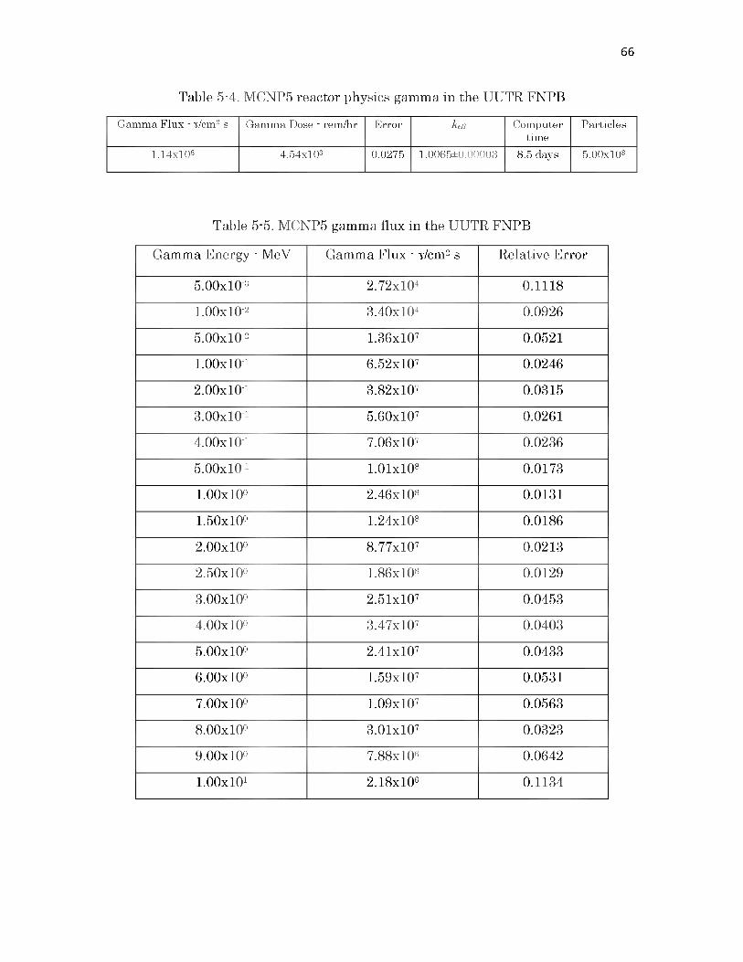
66
Table 5-4. MCNP5 reactor physics gamma in the UUTR FNPB
Gamma Flux - i/cm2 s Gamma Dose - rem/hr Error k e t f Computertime
Particles
1.14x10⁸ 4.54x10³ 0.0275 1.0065±0.00003 8.5 days 5.00x10⁸
Table 5-5. MCNP5 gamma flux in the UUTR FNPB
Gamma Energy - MeV Gamma Flux - i/cm2 s Relative Error
5.00x10'3 2.72x10⁴ 0.1118
1.00x10⁻² 3.40x10⁴ 0.0926
5.00x10'2 1.36x10⁷ 0.0521
1.00x10⁻¹ 6.52x10⁷ 0.0246
2.00x10⁻¹ 3.82x10⁷ 0.0315
3.00x10⁻¹ 5.60x10⁷ 0.0261
4.00x10⁻¹ 7.06x10⁷ 0.0236
5.00x10⁻¹ 1.01x10⁸ 0.0173
1.00x100 2.46x10⁸ 0.0131
1.50x10° 1.24x10⁸ 0.0186
2.00x10° 8.77x10⁷ 0.0213
2.50x100 1.86x10⁸ 0.0129
3.00x100 2.51x10⁷ 0.0453
4.00x100 3.47x10⁷ 0.0403
5.00x100 2.41x10⁷ 0.0433
6.00x100 1.59x10⁷ 0.0531
7.00x100 1.09x10⁷ 0.0563
8.00x100 3.01x10⁷ 0.0323
9.00x100 7.88x10⁶ 0.0642
1.00x101 2.18x10⁶ 0.1134
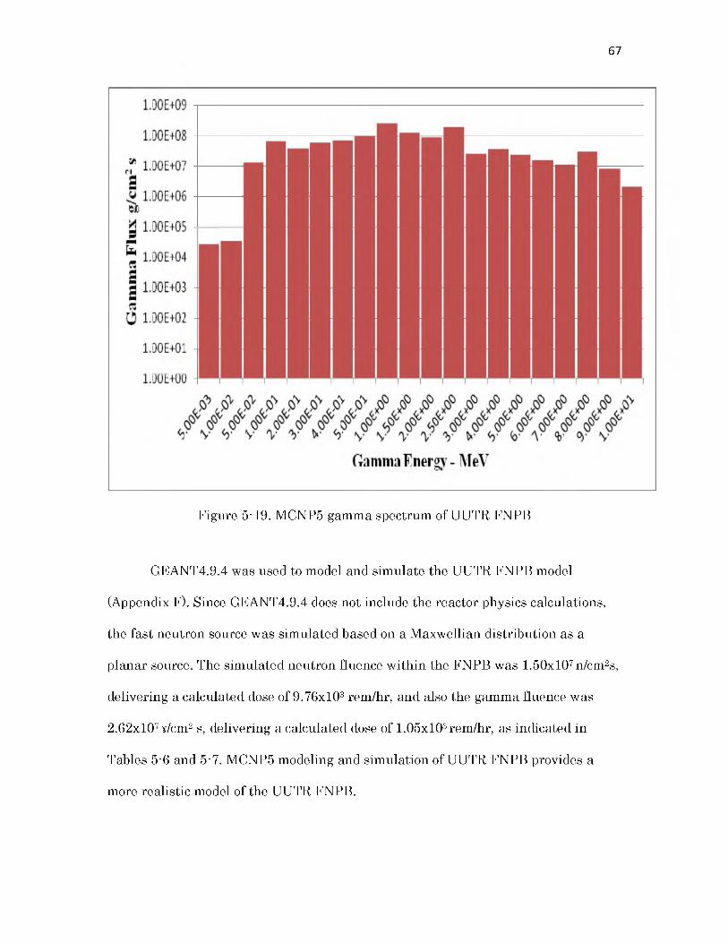
67
Figure 5-19. MCNP5 gamma spectrum of UUTR FNPB
GEANT4.9.4 was used to model and simulate the UUTR FNPB model
(Appendix F). Since GEANT4.9.4 does not include the reactor physics calculations,
the fast neutron source was simulated based on a Maxwellian distribution as a
planar source. The simulated neutron fluence within the FNPB was 1.50x10⁷ n/cm2s,
delivering a calculated dose of 9.76x10³ rem/hr, and also the gamma fluence was
2.62x10⁷ i/cm2 s, delivering a calculated dose of 1.05x10³ rem/hr, as indicated in
Tables 5-6 and 5-7. MCNP5 modeling and simulation of UUTR FNPB provides a
more realistic model of the UUTR FNPB.

68
Table 5-6. GEANT4 summary of UUTR FNPB simulation
Neutron Flux n/cm2 s
Neutron Dose rem/hr
Gamma Flux i/cm2 s
Gamma Dose rem/hr
1.50x10⁷ 9.76x10³ 2.62x10⁷ 1.05x10³
Table 5-7. GEANT4 Simulation of neutron and gamma fluence in the UUTR FNPB
Energy - MeV Neutron Flux n/cm2 s
Gamma Flux i/cm2 s
5.00x10'3 1.31x10⁵ 6.26x1031.00x10-2 3.21x10⁵ 7.83x1035.00x10-2 3.16x10⁵ 3.14x1061.00x10"1 1.08x10⁶ 1.50x1072.00x10'1 5.68x10⁵ 8.79x1063.00x10'1 1.55x10⁶ 1.29x1074.00x10'1 9.48x10⁵ 1.62x1075.00x10'1 1.26 x10⁶ 2.31x1071.00x100 7.94x10⁵ 5.66x1071.50x100 6.58x10⁵ 2.86x1072.00x100 3.59x10⁵ 2.02x1072.50x100 2.38x10⁶ 4.27x1073.00x100 1.49x10⁶ 5.78x1064.00x100 1.08x10⁶ 7.99x1065.00x100 7.04x10⁵ 5.55x1066.00x100 4.99x10⁵ 3.65x1067.00x100 4.38x10⁵ 2.50x1068.00x100 1.51x10⁵ 6.93x1069.00x100 5.98x10⁴ 1.81x1061.00x101 6.34x10⁴ 5.02x10⁵

Comparison of MCNP5 simulation of UUTR FNPB with GEANT4 as shown
in Table 5-8 indicates that MCNP5 gives a more realistic model of the fast neutron
pencil beam with a neutron and gamma flux of 6.52x10⁷ n/cm2s and 1.14x10⁸ x /cm2s,
respectively, while the neutron and gamma flux recorded in GEANT4 were 1.50x10⁷
n/cm2 s and 2.62x10⁷ x/cm2 s, respectively. The results indicate that both the neutron
and gamma flux recorded via GEANT4 simulations were much less than MCNP5
simulation.
5.7. Comparison of UUTR FNPB Design with Other Fast Neutron Pencil Beam Facilities
Fast Neutron Pencil Beam (FNPB) facilities are applied in a couple of fields;
most common amongst the applications are Fast Neutron Therapy for the cure of
cancer and tumors and also for studying the radiation effects on electronic
components’ displacement damage and ionization, as discussed in Chapter 4.
Research conducted by E. Bourhis-Martin [35] at the University of Essen,
Strahlenklinik, Germany on the validation of a fast neutron pencil beam model-
based treatment planning
69
Table 5-8. Comparison of MCNP5 and GEANT4.9.4 Simulation of UUTR FNPB
MCNP5Neutron Flux -
n/cm2 sNeutron Dose -
rem/hrGamma Flux -
x/cm2 sGamma Dose -
rem/hr6.52x107 4.24x10⁴ 1.14x10⁸ 4.54x10³
Preliminary GEANT4.9.4 SimulationNeutron Flux -
n/cm2 sNeutron Dose -
rem/hrGamma Flux -
x/cm2 sGamma Dose -
rem/hr1.50x107 9.76x10³ 2.62x10⁷ 1.05x10³

70
system for fast neutron therapy shows that the estimated fast neutron flux was
within a range of ~106 to 108 n/cm2s, as explained in Chapter 4. Results obtained
from the UUTR FNPB simulation, explained in Chapter 5, shows that the simulated
neutron flux obtained was 6.52x10⁷ n/cm2s, which is well within the estimated range
of neutron flux obtained in existing facilities. Figure 5-20 depicts the comparison of
fast neutron spectrum obtained from MCNP5 simulation of UUTR FNPB with fast
neutron spectrum beam from research by Thomas B. Ucherl [43], showing that the
two spectra have high neutron flux at fast neutron energy.
Calculated fast neutron beam spectrum
FRM-II. , *[TliomasB.ucherl eta! Applied Radiation
and Isotopes 61 (2004)]
Figure 5-20. Comparison of UUTR FNPB spectrum with literature. Adapted from[43]

CHAPTER 6
CONCLUSION AND FUTURE WORK
6.1. Conclusion
The first objective of this thesis was to benchmark different versions of
GEANT4 against experimental measurements and the MCNP5 model, pertaining to
photon transport and interactions. Different versions of the GEANT4 codes (4.9.2,
4.9.3, and 4.9.4) were used to simulate the experimental set up, as described in
Chapter 4. The results obtained from the simulations of different versions of
GEANT4 were benchmarked against MCNP5 code as well, in addition to data
obtained in the experiment. Gamma dose rate measured one foot away from the
cesium source 27 mrem/hr decreased with distance away from the source 0.6 mR/hr.
Even though the GEANT4 versions had different physics models implemented for
photon interactions, the simulations of GEANT4 versions presented good agreement
with experimental data and MCNP5 simulation. Statistical analysis of error
propagation with both GEANT4 and MCNP5 indicates good accuracy with dose rate
measured close to the source as compared to a further distance away from the
detector (this is due to particle angular dispersion as the particle traverses distant
away from the source). Also, a comparison of GEANT4 and MCNP5 simulation of
neutron interactions at thermal and fast neutron energies of 0.025 eV and 2 MeV,
respectively, were assessed for selected materials (lead, boron-10, and paraffin).

Comparison of simulations showed good agreement between GEANT4 and MCNP5
simulation codes for neutron interactions.
The second objective was to develop a preliminary model of Fast Neutron
Pencil Beam Facility at the UUTR using MCNP5 and GEANT4.9.4. The fast neutron
source was modeled in MCNP5 by running reactor physics simulations of the UUTR
reactor core, while the fast neutron source in GEANT4.9.4 was simulated with a
Maxwellian distribution as a planar source. The fast neutron flux obtained in
MCNP5 simulation of the FNPB was 6.52x10⁷ n/cm2s, delivering a neutron dose of
4.24x10⁴ rem/hr. The neutron spectrum, as discussed in Chapter 5, indicates that the
maximum fast neutron flux obtained with the MCNP5 was at neutron energy of 1
MeV. MCNP5 gamma neutron flux of the UUTR FNPB was 1.14x10⁷ i/cm2s,
delivering a gamma dose of 4.54x10³ rem/hr. The gamma flux in the FNPB was
emitted from the nuclear fission reaction in the reactor core. GEANT4.9.4
simulation indicates that the neutron fluence within the FNPB was 1.50x10⁷ n/cm2s,
delivering a calculated dose of 9.76x10⁷ rem/hr, and also, the gamma fluence was
2.62x10⁷ i/cm2s, delivering a calculated dose of 1.05x10³ rem/hr.
In conclusion, MCNP5 modeling and simulation of UUTR FNPB provides a
more realistic model of the UUTR FNPB since it can be used for reactor physics
simulations to therefore give a more realistic prediction of the design.
72
6.2. Recommendations for Future Work
Developing a final design of a fast neutron pencil beam (FNPB) facility at the
UNEP UUTR would enable an introduction of a wide range of experiments which
might not be feasible with the current neutron irradiation ports, such as, but not
limited to:
• Study of biological effect of fast neutrons on biological tissue and cells.
• Study of radiation damage to materials, and real-time analysis of radiation
effect of materials.
• Study of fast neutron interaction effects on electrical components, and real
time analysis of electric circuits in electrical devices.
• Elemental analysis of various samples.
However, a complete optimized design of the FNPB facility will have to be
performed, modeled, and built into the UUTR research reactor in order to be able to
perform feasible scientific experiments, as mentioned above.
This thesis focused on the preliminary design of the fast neutron pencil beam
facility, and further research has to be performed to optimize the UUTR FNPB
model, such as but not limited to, the following;
• Further research concerning different type of compounds that could be used
for collimation of fast neutrons such as borated polyethylene, borated
graphite, or borated wood could be assessed.
• The gamma flux and gamma dose rate calculated in the preliminary design of
UUTR FNPB sample holder was very high; therefore, further research
73
pertaining to good shielding material properties for attenuating gamma
particles from the FNPB model should be done.
• Feasibility analysis of the optimization design of the fast neutron pencil beam
should be re-examined to enhance the fast neutron flux within the FNPB.
Further improvement of the design will enhance the neutron flux and increase the
wide range of research experiments that could be performed with the UUTR FNPB.
74

APPENDIX A
MCNP5 INPUT FILE FOR PHOTON EXPERIMENT

76
c **************************************************************
C BENCHMARK RESEARCH -CHRIS ADJEI
C **************************************************************
1 1 -1.29 -1 -5 4 imp:p=1 $Air gap
2 2 -10.29 -2 -7 6 #1 imp:p=1 $Lead shielding
3 3 -8.06 -3 -7 6 #2 #1 imp:p=1 $StainlessSteeL
4 4 -3.667 8 -9 -10 11 -12 13 imp:p=2 $Detector
5 1 -1.29 14 -15 -16 17 18 -19 #4 #3 #2 #1 imp:p=1 $world volume
6 0 -14:15:-17:16:-18:19 imp:p=0 $ Outside
1 cz 0.721875 $ cell 1 - Air gap in Pig,
4 pz -6.0325 $ cell 1 - bottom of air gap in pig
5 pz -1.95 $ cell 1 - top of air gap in pig
2 cz 2.06375 $ cell 2 - radius of lead
6 pz -7.9375 $ cell 2 - bottom of lead shielding
7 pz 7.9375 $ cell 2 - top of lead shielding
3 cz 2.38125 $ cell 3 - radius of stianlesssteel
8 py -1.27 $ cell 4 - detector side on -y-axis
9 py 1.27 $ cell 4 - detector side on +y-axis
10 px -32.86125 $ cell 4 - detector side on x-axis
11 px -35.40125 $ cell 4 - detector side on y-axis
12 pz 1.27 $ cell 4 - detector side on +z-axis
13 pz -1.27 $ cell 4 - detector side on -Z-axis
14 py -10.0 $ cell 5 - world volume y-axis Box
15 py 10.0 $ cell 5 - world volume y-axis Box
16 pz 20.0 $ cell 5 - world volume z-axis Box

77
17 pz -10.0 $ cell 5 - world volume z-axis Box
18 px -50.0 $ cell 5 - world volume x-axis Box
19 px 10.0 $ cell 5 - world volume x-axis Box
mode p
SDEF ERG=0.6617 POS=0 0 -5.0 AXS= 0 0 1 RAD=d1 EXT=d2 PAR=2
SI1= 0 0.5
SP1= -21 0
SI2= -5.0 -4.0
SP2= -21 0
m1 7014 -0.78084
8016 -0.2094
18040 -0.00976
m2 82207 -1.0
m3 6012 -0.001
14028 -0.007
24052 -0.18
25055 -0.01
26056 -0.712
28059 -0.09
m4 11023 -0.153373
53127 -0.846627
F6:P 4
*F8:P 4
E8 0 1E-5 1E-1 2E-1 3E-1 4E-1 5E-1 6E-1 6.617E-1
FM6 6.845E8
de6 0.01 0.03 0.05 0.07 0.10 0.15 0.20 0.25 0.30 0.35

78
0.40 0.45 0.50 0.55 0.60 0.65 0.70 0.80 1.00 1.40
1.80 2.20 2.60 2.80 3.25 3.75 4.25 4.75 5.00
df6 3.96e-6 5.82e-7 2.90e-7 2.58e-7 2.83e-7 3.79e-7
5.01e-7 6.31e-7 7.59e-7 8.78e-7 9.85e-7 1.08e-6
1.17e-6 1.27e-6 1.36e-6 1.44e-6 1.52e-6 1.68e-6
1.98e-6 2.51e-6 2.99e-6 3.42e-6 3.82e-6 4.01e-6
4.41e-6 4.83e-6 5.23e-6 5.60e-6 5.80e-6
nps 1000000000

APPENDIX B
GEANT4.9.4 INPUT FILE FOR PHOTON EXPERIMENT

80
#include "ExN02DetectorConstruction.hh"
#include "G4Material.hh"
#include "G4Element.hh"
#include "G4Box.hh"
#include "G4VSolid.hh"
#include "G4Tubs.hh"
#include "G4Orb.hh"
#include "G4LogicalVolume.hh"
#include "G4ThreeVector.hh"
#include "G4PVPlacement.hh"
#include "G4NistManager.hh"
#include "G4VisAttributes.hh"
//...oooOO0OOooo........oooOO0OOooo........oooOO0OOooo........oooOO0OOooo
ExN02DetectorConstruction::ExN02DetectorConstruction()
{
expHall_x = expHall_y = expHall_z = 10*cm;
// lcylin_a = 0.*deg;
// lcylin_b = 360.*deg;
bubble_x = 1*cm;
bubble_y = 2*cm;
bubble_z = 2*cm;
// bubble_a = 0.*deg;
// bubble_b = 360.*deg;}
//...oooOO0OOooo........oooOO0OOooo........oooOO0OOooo........oooOO0OOooo
ExN02DetectorConstruction::~ExN02DetectorConstruction(){;}
//...oooOO0OOooo........oooOO0OOooo........oooOO0OOooo........oooOO0OOooo

81
G4VPhysicalVolume* ExN02DetectorConstruction::Construct()
{
// -------------Materials --------------
G4double a, z, density;
G4int nelements, natoms;
G4int ncomponents;
G4double fractionmass, temperature, pressure;
//Vacuum
pressure = 3.e-18*pascal; temperature = 293.15*kelvin;
density = universe_mean_density;
G4Material* Vacuum = new G4Material("Vacuum", 1., 1.01*g/mole, density, kStateGas,temperature,pressure);
// Use NIST database for elements and materials whereever possible.
G4NistManager* man = G4NistManager::lnstance();
man->SetVerbose(1);
G4Element* C = man->FindOrBuildElement("C");
G4Element* Si = man->FindOrBuildElement("Si");
G4Element* Cr = man->FindOrBuildElement("Cr");
G4Element* Mn = man->FindOrBuildElement("Mn");
G4Element* Fe = man->FindOrBuildElement("Fe");
G4Element* Ni = man->FindOrBuildElement("Ni");
G4Element* Na = man->FindOrBuildElement("Na");
G4Element* I = man->FindOrBuildElement("I");
G4Element* Cd = man->FindOrBuildElement("Cd");
G4Element* Al = man->FindOrBuildElement("Al");
G4Element* B = man->FindOrBuildElement("B");

82
G4Material* StainlessSteel = new G4Material("StainlessSteel", density= 8.06*g/cm3, ncomponents=6);
StainlessSteel->AddElement(C, fractionmass=0.001);
StainlessSteel->AddElement(Si, fractionmass=0.007);
StainlessSteel->AddElement(Cr, fractionmass=0.18);
StainlessSteel->AddElement(Mn, fractionmass=0.01);
StainlessSteel->AddElement(Fe, fractionmass=0.712);
StainlessSteel->AddElement(Ni, fractionmass=0.09);
G4Material* SodiumIodide = new G4Material("SodiumIodide", density= 3.667*g/cm3, ncomponents=2);
SodiumIodide->AddElement(Na, fractionmass=0.153373);
SodiumIodide->AddElement(I, fractionmass=0.846627);
G4Material* Cadmium = new G4Material("Cadmium", density= 7.996*g/cm3, ncomponents=1);
Cadmium - >AddElement(C d, fr actionmass=1.0);
G4Material* Boron10 = new G4Material("Boron10", density= 2.08*g/cm3, ncomponents=1);
Boron 10- >AddElement(B, fr actionmass=1.0);
// Air
G4Element* Pb = new G4Element("Lead", "Pb", z=82 , a=207*g/mole);
G4Material* Lead = new G4Material("Lead", density=11.354*g/cm3, nelements=1);
Lead->AddElement(Pb, 100.*perCent);
G4Element* N = new G4Element("Nitrogen", "N", z=7 , a=14.01*g/mole);
G4Element* O = new G4Element("Oxygen" , "O", z=8 , a=16.00*g/mole);
G4Material* Air = new G4Material("Air", density=1.29*mg/cm3, nelements=2);
Air->AddElement(N, 70.*perCent);
Air->AddElement(O, 30.*perCent);
// Water

83
G4Element* H = new G4Element("Hydrogen", "H", z=1 , a=1.01*g/mole);
G4Material* Water = new G4Material("Water", density= 1.0*g/cm3, nelements=2);
Water->AddElement(H, 2);
Water->AddElement(O, 1);
G4Material* Sapphire = new G4Material("Sapphire",density= 4.*g/cm3, ncomponents=2);
Sapphire->AddElement(Al, natoms=2);
Sapphire->AddElement(O , natoms=3);
// Paraffin - Polythelene
G4Material* Paraffin = new G4Material("Paraffin", density= 0.94*g/cm3, nelements=2);
Paraffin->AddElement(C, 85.6*perCent);
Paraffin->AddElement(H, 14.4*perCent);
// The experimental Hall
G4Box* expHall_box = new G4Box("World",expHall_x,expHall_y,expHall_z);
G4LogicalVolume* expHall_log = new G4LogicalVolume(expHall_box,Vacuum,"World",0,0,0);
G4VPhysicalVolume* expHall_phys = new G4PVPlacement(0,G4ThreeVector(),expHall_log,"World",0,false,0);
// The Air Bubble
G4Box* bubbleAir_box = new G4Box("Bubble",bubble_x,bubble_y,bubble_z);
G4LogicalVolume* bubbleAir_log = new G4LogicalVolume(bubbleAir_box,Paraffin,"Bubble",0,0,0);
G4VPhysicalVolume* bubbleAir_phys = new G4PVPlacement(0,G4ThreeVector(- 4*cm,0,0),bubbleAir_log,"Bubble",
expHall_log,false,0);

APPENDIX C
MCNP5 INPUT FILE FOR NEUTRON INTERACTION
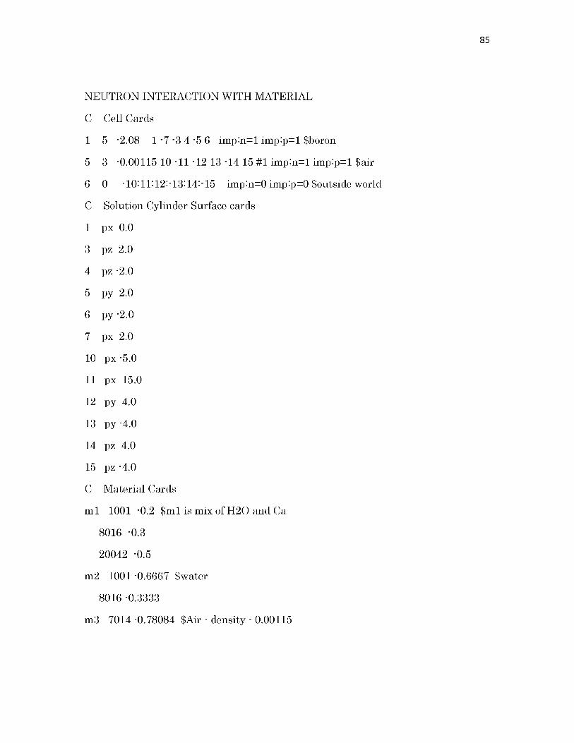
85
NEUTRON INTERACTION WITH MATERIAL
C Cell Cards
1 5 -2.08 1 -7 -3 4 -5 6 imp:n=1 imp:p=1 $boron
5 3 -0.00115 10 -11 -12 13 -14 15 #1 imp:n=1 imp:p=1 $air
6 0 -10:11:12:-13:14:-15 imp:n=0 imp:p=0 $outside world
C Solution Cylinder Surface cards
I px 0.0
3 pz 2.0
4 pz -2.0
5 py 2.0
6 py -2.0
7 px 2.0
10 px -5.0
II px 15.0
12 py 4.0
13 py -4.0
14 pz 4.0
15 pz -4.0
C Material Cards
m1 1001 -0.2 $m1 is mix of H2O and Ca
8016 -0.3
20042 -0.5
m2 1001 -0.6667 $water
8016 -0.3333
m3 7014 -0.78084 $Air - density - 0.00115

86
8016 -0.2094
18040 -0.00976
m4 1001.66c -0.143711 $polyethylene - density 0.94
8016.66c -0.856289
m5 5010.66c -1.0 $Boron - density 2.08
m8 82000.50c -1.0 $ Pb - density 11.354
SDEF PAR=1 ERG=2.5e-8 POS=0 0 0 AXS= 1 0 0 EXT=0 RAD=d1 VEC= 1 0 0 DIR= 1
SI1 0 0.2
SP1 -21 1
c boroncell<--energy deposited (MeV/g)
F06:n 1
F16:p 1
F04:n 1
F14:p 1
mode n p
nps 1e7

APPENDIX D
GEANT4.9.4 INPUT FILE FOR NEUTRON INTERACTION

88
//....oooOO0OOooo....... oooOO0OOooo........oooOO0OOooo........oooOO0OOooo
#include "ExN02DetectorConstruction.hh"
#include "G4Material.hh"
#include "G4Element.hh"
#include "G4Box.hh"
#include "G4VSolid.hh"
#include "G4Tubs.hh"
#include "G4Orb.hh"
#include "G4LogicalVolume.hh"
#include "G4ThreeVector.hh"
#include "G4PVPlacement.hh"
#include "G4NistManager.hh"
#include "G4VisAttributes.hh"
//...oooOO0OOooo........oooOO0OOooo........oooOO0OOooo........oooOO0OOooo
ExN02DetectorConstruction::ExN02DetectorConstruction()
{
expHall_x = expHall_y = expHall_z = 10*cm;
bubble_x = 1*cm;
bubble_y = 2*cm;
bubble_z = 2*cm;
}
//...oooOO0OOooo........oooOO0OOooo........oooOO0OOooo........oooOO0OOooo
ExN02DetectorConstruction::~ExN02DetectorConstruction(){;}
G4VPhysicalVolume* ExN02DetectorConstruction::Construct()

89
{
// -------------Materials --------------
G4double a, z, density;
G4int nelements, natoms;
G4int ncomponents;
G4double fractionmass, temperature, pressure;
//Vacuum
pressure = 3.e-18*pascal; temperature = 293.15*kelvin;
density = universe_mean_density;
G4Material* Vacuum = new G4Material("Vacuum", 1., 1.01*g/mole, density, kStateGas,temperature,pressure);
// Use NIST database for elements and materials whereever possible.
G4NistManager* man = G4NistManager::Instance();
man->SetVerbose(1);
G4Element* C = man->FindOrBuildElement("C");
G4Element* Si = man->FindOrBuildElement("Si");
G4Element* Cr = man->FindOrBuildElement("Cr");
G4Element* Mn = man->FindOrBuildElement("Mn");
G4Element* Fe = man->FindOrBuildElement("Fe");
G4Element* Ni = man->FindOrBuildElement("Ni");
G4Element* Na = man->FindOrBuildElement("Na");
G4Element* I = man->FindOrBuildElement("I");
G4Element* Cd = man->FindOrBuildElement("Cd");
G4Element* Al = man->FindOrBuildElement("Al");
G4Element* B = man->FindOrBuildElement("B");
G4Material* StainlessSteel = new G4Material("StainlessSteel", density= 8.06*g/cm3, ncomponents=6);
90
StainlessSteel->AddElement(C, fractionmass=0.001);
StainlessSteel->AddElement(Si, fractionmass=0.007);
StainlessSteel->AddElement(Cr, fractionmass=0.18);
StainlessSteel->AddElement(Mn, fractionmass=0.01);
StainlessSteel->AddElement(Fe, fractionmass=0.712);
StainlessSteel->AddElement(Ni, fractionmass=0.09);
G4Material* SodiumIodide = new G4Material("SodiumIodide", density= 3.667*g/cm3, ncomponents=2);
SodiumIodide->AddElement(Na, fractionmass=0.153373);
SodiumIodide->AddElement(I, fractionmass=0.846627);
G4Material* Cadmium = new G4Material("Cadmium", density= 7.996*g/cm3, ncomponents=1);
Cadmium - >AddElement(C d, fr actionmass=1.0);
G4Material* Boron10 = new G4Material("Boron10", density= 2.08*g/cm3, ncomponents=1);
Boron 10- >AddElement(B, fr actionmass=1.0);
G4Element* Pb = new G4Element("Lead", "Pb", z=82 , a=207*g/mole);
G4Material* Lead = new G4Material("Lead", density=11.354*g/cm3, nelements=1);
Lead->AddElement(Pb, 100.*perCent);
G4Element* N = new G4Element("Nitrogen", "N", z=7 , a=14.01*g/mole);
G4Element* O = new G4Element("Oxygen" , "O", z=8 , a=16.00*g/mole);
G4Material* Air = new G4Material("Air", density=1.29*mg/cm3, nelements=2);
Air->AddElement(N, 70.*perCent);
Air->AddElement(O, 30.*perCent);
// Water
G4Element* H = new G4Element("Hydrogen", "H", z=1 , a=1.01*g/mole);
G4Material* Water = new G4Material("Water", density= 1.0*g/cm3, nelements=2);

91
Water->AddElement(H, 2);
Water->AddElement(O, 1);
G4Material* Sapphire = new G4Material("Sapphire",density= 4.*g/cm3, ncomponents=2);
Sapphire->AddElement(Al, natoms=2);
Sapphire->AddElement(O , natoms=3);
// Paraffin - Polythelene
G4Material* Paraffin = new G4Material("Paraffin", density= 0.94*g/cm3, nelements=2);
Paraffin->AddElement(C, 85.6*perCent);
Paraffin->AddElement(H, 14.4*perCent);
// The experimental Hall
G4Box* expHall_box = new G4Box("World",expHall_x,expHall_y,expHall_z);
G4LogicalVolume* expHall_log = new G4LogicalVolume(expHall_box,Vacuum,"World",0,0,0);
G4VPhysicalVolume* expHall_phys = new G4PVPlacement(0,G4ThreeVector(),expHall_log,"World",0,false,0);
// The Air Bubble
G4Box* bubbleAir_box = new G4Box("Bubble",bubble_x,bubble_y,bubble_z);
G4LogicalVolume* bubbleAir_log = new G4LogicalVolume(bubbleAir_box,Paraffin,"Bubble",0,0,0);
G4VPhysicalVolume* bubbleAir_phys = new G4PVPlacement(0,G4ThreeVector(- 4*cm,0,0),bubbleAir_log,"Bubble",
expHall_log,false,0);
return expHall_phys;}
//...oooOO0OOooo........oooOO0OOooo........oooOO0OOooo........oooOO0OOooo.....

APPENDIX E
MCNP5 INPUT FILE OF UUTR FNPB
93
UUTR FNPB PRILIMENARY MODEL
c New SS Fuel
100 1 -5.636 -2 11 -12 u=1 imp:n=1 imp:p=1 $Fuel Meat
101 2 -1.70 -2 12 -14 u=1 imp:n=1 imp:p=1 $Up Graphite
102 2 -1.70 -2 13 -11 u=1 imp:n=1 imp:p=1 $Down Graphite
103 3 -7.92 (-1 15 -16) (2:-13:14) u=1 imp:n=1 imp:p=1 $Cladding
104 4 -1.0 1:-15:16 92 -93 u=1 imp:n=1 imp:p=1 $H2O
c Old SS Fuel
110 like 100 but mat=12 rho=-5.636 u=2 imp:n=1 imp:p=1 $Fuel Meat
111 like 101 but u=2 imp:n=1 imp:p=1 $Up Graphite
112 like 102 but u=2 imp:n=1 imp:p=1 $Down Graphite
113 like 103 but u=2 imp:n=1 imp:p=1 $Cladding
114 like 104 but u=2 imp:n=1 imp:p=1 $H2O
c Al Fuel
120 5 -6.143 -3 21 -22 u=3! imp:n=1 imp:p=1 $Fuel Meat
121 2 -1.70 -3 22 -24 u=3 imp:n=1 imp:p=1 $Up Graphite
122 2 -1.70 -3 23 -21 u=3 imp:n=1 imp:p=1 $Down Graphit
123 6 -2.70 (-1 25 -26) (3:-23:24) u=3 imp:n=1 imp:p=1 $Cladding
124 4 -1.0 1:-25:26 92 -93 u=:3 imp:n=1 imp:p=1 $H2O
c Instrumental Fuel
130 like 110 but u=4 imp:n=1 imp:p=1 $Fuel Meat
131 like 111 but u=4 imp:n=1 imp:p=1 $Up Graphite
132 like 112 but u=4 imp:n=1 imp:p=1 $Down Graphite
133 like 113 but u=4 imp:n=1 imp:p=1 $Cladding
134 like 114 but u=4 imp:n=1 imp:p=1 $H2O
c Graphite

94
140 2 -1.70 -3 23 -24
143 like 123 but
144 like 124 but
c Heavy Water
150 7 -1.056 -3 23 -24
153 like 123 but
154 like 124 but
c Water
160 4 -1.0 -1 92 -93
161 4 -1.0 1 92 -93
c Safety Control Rod
170 9 -2.52 -46 11 -93
171 6 -2.7 46 -47 11 -93
172 4 -1.0 (47 -50 11 -93):(-
173 6 -2.7 50 -1 92 -93
174 4 -1.0 1 92 -93
c Shim Control Rod
180 9 -2.52 -46 11 -93
181 6 -2.7 46 -47 11 -93
182 4 -1.0 (47 -50 11 -93):(-
183 6 -2.7 50 -1 92 -93
184 4 -1.0 1 92 -93
c Reg Control Rod
190 9 -2.52 -48 11 -93
191 6 -2.7 48 -49 11 -93
192 4 -1.0 (49 -50 11 -93):(-
u=6 imp:n=1 imp:p=1 $Graphite
u=6 imp:n=1 imp:p=1 $Cladding
u=6 imp:n=1 imp:p=1 $H2O
u=7 imp:n=1 imp:p=1 $D2O
u=7 imp:n=1 imp:p=1 $Cladding
u=7 imp:n=1 imp:p=1 $H2O
u=8 imp:n=1 imp:p=1 $H2O
u=8 imp:n=1 imp:p=1 $H2O
u=10 imp:n=1 imp:p=1 $B4C
u=10 imp:n=1 imp:p=1 $Al Cladding
50 -11 92) u=10 imp:n=1 imp:p=1 $H2O
u=10 imp:n=1 imp:p=1 $Al Tube
u=10 imp:n=1 imp:p=1 $H2O
u=11 imp:n=1 imp:p=1 $B4C
u=11 imp:n=1 imp:p=1 $Al Cladding
50 -11 92) u=11 imp:n=1 imp:p=1 $H2O
u=11 imp:n=1 imp:p=1 $Al Tube
u=11 imp:n=1 imp:p=1 $H2O
u=12 imp:n=1 imp:p=1 $B4C
u=12 imp:n=1 imp:p=1 $Al Cladding
50 -11 92) u=12 imp:n=1 imp:p=1 $H2O

95
193 6 -2.7 50 -1 92 -93 u=12 imp:n=1 imp:p=1 $Al Tube
194 4 -1.0 1 92 -93 u=12 imp:n=1 imp:p=1 $H2O
c Empty Control Rod
196 4 -1.0 -50 92 -93 u=5 imp:n=1 imp:p=1 $H2O
197 6 -2.7 50 -1 92 -93 u=5 imp:n=1 imp:p=1 $Al Tube
198 4 -1.0 1 92 -93 u=5 imp:n=1 imp:p=1 $H2O
c Brand New SS Fuel, more U235
c 310 like 100 but mat=5 rho=-5.781 u=15 imp:n=1 imp:p=1 $Fuel Meat
c 311 like 101 but u=15 imp:n=1 imp:p=1 $Up Graphite
c 312 like 102 but u=15 imp:n=1 imp:p=1 $Down Graphite
c 313 like 103 but u=15 imp:n=1 imp:p=1 $Cladding
c 314 like 104 but u=15 imp:n=1 imp:p=1 $H2O
c Lattice
200 4 -1.0 -101 102 -103 104 -105 106 92 -93 lat=2 u=9
fill=-7:7 -7:7 0:0
0 0 0 0 0 0 0 9 9 9 9 9 9 9 9
0 0 0 0 0 0 9 8 7 8 7 8 7 8 9
0 0 0 0 0 9 3 2 3 1 1 3 2 7 9
0 0 0 0 9 1 3 1 1 1 1 3 3 8 9
0 0 0 9 1 1 3 1 3 1 5 3 3 7 9
0 0 9 3 1 1 4 1 2 2 1 2 3 7 9
0 9 3 3 1 3 2 2 2 4 2 3 3 7 9
9 8 7 2 5 1 1 5 1 1 8 3 1 6 9
9 8 7 1 2 2 1 1 1 2 1 3 6 9 0
9 8 7 1 3 8 2 2 1 3 1 6 9 0 0
9 8 7 1 1 2 2 5 3 3 6 9 0 0 0

96
9 8 7 8 1 1 1 1 1 6 9 0 0 0 0
9 8 6 6 6 6 6 6 6 9 0 0 0 0 0
9 8 8 8 8 8 8 8 9 0 0 0 0 0 0
9 9 9 9 9 9 9 9 0 0 0 0 0 0 0 imp:n=1 imp:p=1
201 4 -1.0 -111 112 -113 114 -115 116 92 -93 fill=9 imp:n=1 imp:p=1 $Lattices
202 6 -2.7 (-121 122 -123 124 -125 126) 91 -94
(111:-112:113:-114:115:-116) imp:n=1 imp:p=1 $Al Wall
203Plate
6k
-2.7 -111 112 -113 114 -115 116 91 -92 imp:n=1 imp:p=1 $Lower Al
204 6 Al Plate
-2.7 -111 112 -113 114 -115 116 93 -94 41 43 45 imp:n=1 imp:p=1 $Upper
206 4 -1.0 -131 94 -97 41 43 45 #402 #404 #405 #406 #408 #410 #418
#412 #414 #416 #424 imp:n=1 imp:p=1 $Top Water
207 4 -1.0 -131 96 -91 imp:n=1 imp:p=1 $Bottom Water
208 10 -2.30 -131 -96 95 imp:n=1 imp:p=1 $Bottom Concrete
301 9 -2.52 -40 93 -97 imp:n=1 imp:p=1 $Safety Rod above core region
302 6 -2.7 40 -41 93 -97 imp:n=1 imp:p=1
303 9 -2.52 -42 93 -97 imp:n=1 imp:p=1 $Shim Rod above core region
304 6 -2.7 42 -43 93 -97 imp:n=1 imp:p=1
305 9 -2.52 -44 93 -97 imp:n=1 imp:p=1 $Reg Rod above core region
306 6 -2.7 44 -45 93 -97 imp:n=1 imp:p=1
c FNIF
400 11 -0.00115 -141 #402 #418 #420 #422 imp:n=2 imp:p=2 $ FNIF Air
401 8 -11.34 -140 141 imp:n=1 imp:p=1 $ FNIF Pb
402 8 -11.34 -142 imp:n=1 imp:p=1 $ Lead base of PFNB
404 11 -0.00115 -246 -244 248 imp:n=4 imp:p=4 $ pencil beam inner cone

97
418 6 -2.7 -145 #420 #422 imp:n=2 imp:p=2 $ Aluminum casing of PFNB in FNIF
420 8 -11.34 -147 imp:n=1 imp:p=1 $ Lead block in aluminum casing
422 11 -0.00115 -149 imp:n=4 imp:p=4 $ Air gap in aluminum casing
405 11 -0.00115 -144 imp:n=4 imp:p=4 $ Air Collimator box
406 11 -0.00115 -240 -250 244 imp:n=4 imp:p=4 $ pencil mouth of collimator cylinder
424 17 -2.08 -262 -264 266 imp:n=4 imp:p=4 $ Boron window - PFNB
408 8 -11.34 -252 #410 #406 #424 imp:n=2 imp:p=2 $ SAMPLER CASING
410 11 -0.00115 -254 imp:n=16 imp:p=16 $ Inner sAMPLER holder - AIR
412 14 -0.94 -260 #402 #404 #405 #406 #408 #410 #424 imp:n=2 imp:p=2 $ Collimator box
414 6 -2.7 -256 258 imp:n=2 imp:p=2 $ Aluminum cladding of PFNB
416 17 -2.08 -258 260 imp:n=2 imp:p=2 $boron shielding in collimator
c Heavy water block
500 11 -0.00115 -159 160 -161 imp:n=1 imp:p=1 $ Heavy water Air
501 6 -2.7 159 -158 160 -161 imp:n=1 imp:p=1
502 7 -1.056 158 154 -155 156 157 160 -161 imp:n=1 imp:p=1
503 6 -2.7 (-154:155:-156:-157)
150 -151 152 153 160 -161 imp:n=1 imp:p=1
c
900 4 -1.0 -131 91 -94 140
(-150:151:-152:-153:-160:161)
(121:-122:123:-124:125:-126) #402 #404 #405 #406 #408 #410 #412
#414 #416 #418 #424 imp:n=1 imp:p=1 $Water Arround Core
999 0 131:-95:97 imp:n=0 imp:p=0
C Surface Cards

1
2
3
11
12
13
14
15
16
21
22
23
24
25
26
40
41
42
43
44
45
46
47
48
49
50
98
cz 1.873 $Outer Radius
cz 1.82 $Inner Radius
cz 1.79 $Inner Radius for Aluminum Container
pz -19.05 $SS Fuel Meat Bottom (7.5 inch * 2)
pz 19.05 $SS Fuel Meat Top
pz -29.21 $SS Fuel Graphite Bottom (4 inch)
pz 29.21 $SS Fuel Graphite Top
pz -30.39 $SS Cladding Bottom (1.18 cm)
pz 30.39 $SS Cladding Top (1.18 cm)
pz -17.78 $Al Fuel Meat Bottom (7 inch * 2)
pz 17.78 $Al Fuel Meat Top
pz -27.94 $Al Fuel Graphite Bottom (4 inch)
pz 27.94 $Al Fuel Graphite Top
pz -29.12 $Al Cladding Bottom (1.18 cm)
pz 29.12 $Al Cladding Top (1.18 cm)
c/z 6.555 -11.354 1.00 $Safety Control Rod
c/z 6.555 -11.354 1.11 $Safety Control Rod Claddii
c/z -13.11 0.0 1.00 $Shim Control Rod
c/z -13.11 0.0 1.11 $Shim Control Rod Cladding
c/z 6.555 11.354 0.200 $Reg Control Rod
c/z 6.555 11.354 0.318 $Reg Control Rod Cladding
cz 1.00 $ Safety and Shim Rod in Unit
cz 1.11 $ Safety and Shim Rod in Unit Cladding
cz 0.200 $ Reg Rod in Unit
cz 0.318 $ Reg Rod in Unit Cladding
cz 1.750 $ Inner radius of Al tube for control rod

99
91 pz -33.43 $Lower Plate Bottom
92 pz -30.89 $Lower Plate Top (1 inch)
93 pz 30.89 $Upper Plate Bottom
94 pz 32.79 $Upper Plate Top (0.75 inch)
95 pz -55.0 $Concrete Bottom
96 pz -43.09 $Water Bottom (2 inch)
97 pz 100.0 $Water Top
C Lattice Cells
101 px 2.185
102 px -2.185
103 p 0.5 0.8660254 0 2.185
104 p 0.5 0.8660254 0 -2.185
105 p -0.5 0.8660254 0 2.185
106 p -0.5 0.8660254 0 -2.185
c Frame Boundary
111 p 1.732038 1 0 50.460
112 p 1.732038 1 0 -50.460
113 p 1.732038 -1 0 50.460
114 p 1.732038 -1 0 -50.460
115 py 25.230
116 py -25.230
c Al Wall
121 p 1.732038 1 0 54.270
122 p 1.732038 1 0 -54.270
123 p 1.732038 -1 0 54.270
124 p 1.732038 -1 0 -54.270

100
125 py 27.135
126 py -27.135
C Reflector Surfaces
131 cz 65.0 $ Water reflector
c 131 p 1.732038 1 0 83.259682
c 132 p 1.732038 1 0 -83.259682
c 133 p 1.732038 -1 0 83.259682
c 134 p 1.732038 -1 0 -83.259682
c 135 py 41.629841
c 136 py -41.629841
c FNIF
140 BOX -15.88 -26.77 -30.48 -15.24 26.40 0 -22.00 -12.70 0 0 0 60.96
141 BOX -22.82 -24.91 -30.48 -10.16 17.60 0 -08.80 -05.10 0 0 0 60.96
142 BOX -22.87 -24.86 -30.48 -10.11 17.50 0 -08.75 -05.05 0 0 0 05.08
145 BOX -22.87 -24.86 -25.40 -10.11 17.50 0 -08.75 -05.05 0 0 0 55.88
144 BOX -22.97 -24.96 31.00 -10.01 17.40 0 -08.65 -04.95 0 0 0 20.08
147 BOX -22.97 -24.96 -24.90 -10.01 17.40 0 -08.65 -04.95 0 0 0 02.54
149 BOX -22.97 -24.96 -22.36 -10.01 17.40 0 -08.65 -04.95 0 0 0 52.34
252 BOX -27.66 -21.33 73.00 -05.00 08.50 0 -04.50 -02.70 0 0 0 07.00
254 BOX -28.15 -21.20 73.50 -04.60 08.10 0 -04.10 -02.30 0 0 0 06.00
256 BOX -15.88 -26.77 30.48 -15.24 26.40 0 -22.00 -12.70 0 0 0 50.00
258 BOX -16.88 -26.90 31.00 -14.24 25.40 0 -21.00 -11.70 0 0 0 49.00
260 BOX -17.88 -27.00 31.00 -13.24 24.40 0 -20.00 -10.70 0 0 0 49.00
c Heavy water beside core
150 p 1.732038 1 0 54.270 $ Al oute
151 p 1.732038 1 0 84.670
101
152 py 0.0
153 p 1.732038 -1 0 0.0
154 p 1.732038 1 0 54.670 $ Al outer
155 p 1.732038 1 0 84.270
156 py 0.2
157 p 1.732038 -
158 c/z 30.08 17.37
159 c/z 30.08 17.37
160 pz -30.0
161 pz 30.0
201 pz -18.5
202 pz -17.5
203 pz -16.5
204 pz -15.5
205 pz -14.5
206 pz -13.5
207 pz -12.5
208 pz -11.5
209 pz -10.5
210 pz -9.5
211 pz -8.5
212 pz -7.5
213 pz -6.5
214 pz -5.5
215 pz -4.5
216 pz -3.5
1 0 0.4
5.7 $ Air tub Al wall
5.5 $ Air tub
$ Heavy water top
$ Heavy water bottom

102
217 pz -2.5
218 pz -1.5
219 pz -0.5
220 pz 0.5
221 pz 1.5
222 pz 2.5
223 pz 3.5
224 pz 4.5
225 pz 5.5
226 pz 6.5
227 pz 7.5
228 pz 8.5
229 pz 9.5
230 pz 10.5
231 pz 11.5
232 pz 12.5
233 pz 13.5
234 pz 14.5
235 pz 15.5
236 pz 16.5
237 pz 17.5
238 pz 18.5
240 c/z -32 -19 1.5
244 pz 67.48
246 k/z -32 -19 71.48 0.17 -1
248 pz 51.08

103
250 pz 73
262 c/z -32 -19 1.5
264 pz 73.5
266 pz 73
mode n p
kcode 100000 1.0 100 5000
ksrc -15.2950 -18.9227 0.0000
10.9250 -18.9227 0.0000
-6.5550 -18.9227 0.0000
-2.1850 -18.9227 0.0000
2.1850 -18.9227 0.0000
6.5550 -18.9227 0.0000
10.9250 -18.9227 0.0000
17.4800 -15.1381 0.0000
13.1100 -15.1381 0.0000
-8.7400 -15.1381 0.0000
-4.3700 -15.1381 0.0000
0.0000 -15.1381 0.0000
4.3700 -15.1381 0.0000
8.7400 -15.1381 0.0000
13.1100 -15.1381 0.0000
19.6650 -11.3536 0.0000
15.2950 -11.3536 0.0000
10.9250 -11.3536 0.0000
-6.5550 -11.3536 0.0000
-2.1850 -11.3536 0.0000
104
2.1850 -11.3536 0.0000
10.9250 -11.3536 0.0000
15.2950 -11.3536 0.0000
21.8500 -7.5691 0.0000
8.7400 15.1381 0.0000
13.1100 15.1381 0.0000
m1 1001.66c -0.015896 $ new SS meat, H/Zr=1.6. 0.59% burn-up
40000.66c -0.899104
92235.66c -0.016728
m2 6000.66c 1.0 $ graphite
mt2 grph.60t
m3 6000.66c -0.0004 $ ss cladding
14000.60c -0.0046
24000.50c -0.190
25055.66c -0.009
26000.50c -0.699
28000.50c -0.097
m4 1001.66c 2.0 $ H2O
8016.66c 1.0
mt4 lwtr.60t
m5 1001.66c -0.010 $ Al meat, H/Zr=1.0, 8.91% burnup
40000.66c -0.905
92235.66c -0.01533
92238.66c -0.06967
mt5 h/zr.60t
zr/h.60t

105
m6 13027.66c 1.0 $ Al
m7 1001.66c 0.64 $ D20 (68% atom)
1002.66c 1.36
8016.66c 1.00
m8 82000.50c 1.0 $ Pb
m9 5010.66c -0.1566 $ b4c
5011.66c -0.6264
6000.66c -0.217
m10 1001.66c -0.00619 $ Concrete
6000.66c -0.17520
8016.66c -0.41020
11023.66c -0.00027
12000.66c -0.03265
13027.66c -0.01083
14000.60c -0.03448
19000.66c -0.00114
20000.66c -0.32130
26000.50c -0.00778
m11 7014.66c 0.0000381259 $Air
8016.66c 0.0000095012
18000.59c 0.0000001664
m12 1001.66c -0.015896 $ Old SS meat,
40000.66c -0.899104
92235.66c -0.015354
92238.66c -0.069646
m13 26054.66c -1.0 $iron - density 7.874

106
m14 1001.66c -0.143711 $polyethylene - density 0.94
8016.66c -0.856289
m15 1001.66c -0.148605 $paraffin wax - density 0.93
8016.66c -0.851395
m16 1001.66c -0.06 $wood - density 1.4
8016.66c -0.44
6000.66c -0.50
m17 5010.66c -1.0 $Boron - density 2.08
c New SS Fuel (u=1)
f47:n (130<200[-1 -2 0]<201) (130<200[2 -1 0]<201)
FS47 -201 -202 -203 -204 -205 -206 -207 -208 -209 -210 -211 -212 -213 -214
-215 -216 -217 -218 -219 -220 -221 -222 -223 -224 -225 -226 -227 -228
-229 -230 -231 -232 -233 -234 -235 -236 -237 -238
E54 0 1E-9 5E-9 2.5E-8 1E-7 6.25E-7 2E-6 1E-5 1E-4 5E-4 1E-3 5E-3 0.01 0.05 0.1
0.2 0.3 0.4 0.5 1 1.5 2 2.5 3 4 5 6 7 8 9 10 11 12 13 14 15 16 17 18 19 20
f64:n 410 $ SAMPLER
E64 0 1E-9 5E-9 2.5E-8 1E-7 6.25E-7 2E-6 1E-5 1E-4 5E-4 1E-3 5E-3 0.01 0.05 0.1
0.2 0.3 0.4 0.5 1 1.5 2 2.5 3 4 5 6 7 8 9 10 11 12 13 14 15 16 17 18 19 20
f74:p 410 $ SAMPLER
FMESH84:n GEOM=rec 0RIGIN=-40 -40 -40
IMESH=40 IINTS=40
JMESH=40 JINTS=40
KMESH=40 KINTS=40
EMESH=2.5E-8 6.25E-7 0.1 20 EINTS=1 1 1 1 0UT=ij

APPENDIX F
GEANT4.9.4 INPUT FILE OF UUTR FNPB

108
//...oooOO0OOooo........oooOO0OOooo........oooOO0OOooo.....
ExN02DetectorConstruction::ExN02DetectorConstruction()
{
// world volume
world_x = world_y = world_z = 10*m;
// FNIF-lead
FNIF_x = 12.7*cm;
FNIF_y = 13.5*cm;
FNIF_z = 30.48*cm;
// FNIF-Air
FNIFa_x = 5.08*cm;
FNIFa_y = 8.42*cm;
FNIFa_z = 30.48*cm;
//FNPB - Aluminum casing
FNPBAli_x = 12.7*cm;
FNPBAli_y = 13.5*cm;
FNPBAli_z = 25*cm;
//FNPB - Boron shielding inside FNPB
FNPBB_x = 12.4*cm;
FNPBB_y = 13*cm;
FNPBB_z = 25*cm;
//FNPB - collimator paraffin
FNPBcoll_x = 11.7*cm;
FNPBcoll_y = 12.5*cm;
oooOO0OOooo

109
FNPBcoll_z = 25*cm;
//FNPB - sampler casing
Casing_x = 2.5*cm;
Casing_y = 4*cm;
Casing_z = 3*cm;
//FNPB - sampler casing
sampler_x = 2*cm;
sampler_y = 3.5*cm;
sampler_z = 2.5*cm;
//Pencil tip
pencil_x = 0*cm;
pencil_y = 1.5*cm;
pencil_z = 2.5*cm;
pencil_a = 0.*deg;
pencil_b = 360.*deg;
// Air collimator box
Calor_x = 5.08*cm;
Calor_y = 8.42*cm;
Calor_z = 15*cm;
//cone tip
dx1 =5.08*cm;
dx2 =1.5*cm;
dy1 =8.42*cm;
dy2 =1.5*cm;

110
dz = 5*cm;
//Fuel Box
Fbox_x = 1.8*cm;
Fbox_y = 13.5*cm;
Fbox_z = 30.48*cm;
//fuel pin}
//...oooOO0OOooo........oooOO0OOooo........oooOO0OOooo........oooOO0OOooo
ExN02DetectorConstruction::~ExN02DetectorConstruction(){;}
//...oooOO0OOooo........oooOO0OOooo........oooOO0OOooo........oooOO0OOooo
G4VPhysicalVolume* ExN02DetectorConstruction::Construct()
G4double a, z, density;
G4int nelements, natoms;
G4int ncomponents;
G4double fractionmass, temperature, pressure;
//Define stainless steel
// Use NIST database for elements and materials whereever possible.
G4NistManager* man = G4NistManager::Instance();
man->SetVerbose(1);
G4Element* C = man->FindOrBuildElement("C");
G4Element* Si = man->FindOrBuildElement("Si");
G4Element* Cr = man->FindOrBuildElement("Cr");
G4Element* Mn = man->FindOrBuildElement("Mn");
G4Element* Fe = man->FindOrBuildElement("Fe");
G4Element* Ni = man->FindOrBuildElement("Ni");
111
G4Element* Na = man->FindOrBuildElement("Na");
G4Element* I = man->FindOrBuildElement("I");
G4Element* Cd = man->FindOrBuildElement("Cd");
G4Element* Al = man->FindOrBuildElement("Al");
G4Element* B = man->FindOrBuildElement("B");
G4Material* Cadmium = new G4Material("Cadmium", density= 7.996*g/cm3, ncomponents=1);
Cadmium - >AddElement(C d, fr actionmass=1.0);
G4Material* Boron10 = new G4Material("Boron10", density= 2.08*g/cm3, ncomponents=1);
Boron10->AddElement(B, fractionmass=1.0);
G4Material* Aluminum = new G4Material("Aluminum", density= 2.7*g/cm3, ncomponents=1);
Aluminum->AddElement(Al, fractionmass=1.0);
// Air
G4Element* Pb = new G4Element("Lead", "Pb", z=82 , a=207*g/mole);
G4Material* Lead = new G4Material("Lead", density=11.354*g/cm3, nelements=1);
Lead->AddElement(Pb, 100.*perCent);
G4Element* N = new G4Element("Nitrogen", "N", z=7 , a=14.01*g/mole);
G4Element* O = new G4Element("Oxygen" , "O", z=8 , a=16.00*g/mole);
G4Material* Air = new G4Material("Air", density=1.29*mg/cm3, nelements=2);
Air->AddElement(N, 70.*perCent);
Air->AddElement(O, 30.*perCent);
// Water
G4Element* H = new G4Element("Hydrogen", "H", z=1 , a=1.01*g/mole);
G4Material* Water = new G4Material("Water", density= 1.0*g/cm3, nelements=2);

112
Water->AddElement(H, 2);
Water->AddElement(0, 1);
G4Material* Sapphire = new G4Material("Sapphire",density= 4.*g/cm3, ncomponents=2);
Sapphire->AddElement(Al, natoms=2);
Sapphire->AddElement(0 , natoms=3);
// Paraffin - Polythelene
G4Material* Paraffin = new G4Material("Paraffin", density= 0.94*g/cm3, nelements=2);
Paraffin->AddElement(C, 85.6*perCent);
Paraffin->AddElement(H, 14.4*perCent);
//==========================================================
// Description of FNPB Geometry
//==========================================================
// The WORLD VOLUME
G4Box* world_box = new G4Box("World",world_x,world_y,world_z);
G4LogicalVolume* world_log = new G4LogicalVolume(world_box,Water,"World",0,0,0);
G4VPhysicalVolume* world_phys = new G4PVPlacement(0,G4ThreeVector(),world_log,"World",0,false,0);
// FNIF-Lead
G4VSolid* FINFLead_box = new G4Box("FNIF", FNIF_x, FNIF_y, FNIF_z);
G4LogicalVolume* FINFLead_log = new G4LogicalVolume(FINFLead_box,Lead,"FNIF",0,0,0);
G4VPhysicalVolume* FINFLead_phys = new G4PVPlacement(0,G4ThreeVector(0,0,0),FINFLead_log,"FNIF",
world_log,false,0);

113
// FNIF-Air
G4VSolid* FNIF_Box = new G4Box("FNIF-air",FNIFa_x,FNIFa_y,FNIFa_z);
G4LogicalVolume* FNIF_log = new G4LogicalVolume(FNIF_Box,Air,"FNIF- air",0,0,0);\
G4VPhysicalVolume* FNIF_phys = new G4PVPlacement(0,G4ThreeVector(2.54*cm,0,0),FNIF_log,"FNIF- air",world_log,false,0);
// FNPB-Aluminum
G4VSolid* FNPBAli_box = new G4Box("FNPB-ali", FNPBAli_x, FNPBAli_y, FNPBAli_z);
G4LogicalVolume* FNPBAli_log = new G4LogicalVolume(FNPBAli_box,Aluminum,"FNPB-ali",0,0,0);
G4VPhysicalVolume* FNPBAli_phys = new G4PVPlacement(0,G4ThreeVector(0,0,55.48*cm),FNPBAli_log,"FNPB-ali",
world_log,false,0)
// FNPB-Boron
G4VSolid* FNPBB_box = new G4Box("FNPBBoron", FNPBB_x, FNPBB_y, FNPBB_z);
G4LogicalVolume* FNPBB_log = new G4LogicalVolume(FNPBB_box,Boron10,"FNPBBoron",0,0,0);
G4VPhysicalVolume* FNPBB_phys = newG4PVPlacement(0,G4ThreeVector(0,0,55.48*cm),FNPBB_log,"FNPBBoron",
world_log,false,0);
// FNPB-Collimator
G4VSolid* FNPBcollim_box = new G4Box("collimator", FNPBcoll_x, FNPBcoll_y, FNPBcoll_z);
G4LogicalVolume* FNPBcollim_log = new
G4LogicalVolume(FNPBcollim_box,Paraffin,"collimator",0,0,0);

114
G4VPhysicalVolume* FNPBcollim_phys = newG4PVPlacement(0,G4ThreeVector(0,0,55.48*cm),FNPBcollim_log,"collimator",
world_log,false,0);
G4VSolid* Casing_box = new G4Box("Casing", Casing_x, Casing_y, Casing_z);G4LogicalVolume* Casing_log = new G4LogicalVolume(Casing_box,Lead,"Casing",0,0,0);
G4VPhysicalVolume* Casing_phys = newG4PVPlacement(0,G4ThreeVector(2.54*cm,0,77.48*cm),Casing_log,"Casing",
world_log,false,0);
// Sampler-Air
G4VSolid* sampler_box = new G4Box("sampler", sampler_x, sampler_y, sampler_z);
G4LogicalVolume* sampler_log = new G4LogicalVolume(sampler_box,Air,"sampler",0,0,0);
G4VPhysicalVolume* sampler_phys = newG4PVPlacement(0,G4ThreeVector(2.54*cm,0,77.98*cm),sampler_log,"sampler",
world_log,false,0);
// Pencil tip of colliator
G4Tubs* pencil_tip = new G4Tubs("pencil",pencil_x,pencil_y,pencil_z, pencil_a,pencil_b);
G4LogicalVolume* pencil_log = new G4LogicalVolume(pencil_tip,Air,"pencil",0,0,0);
G4VPhysicalVolume* pencil_phys = new G4PVPlacement(0,G4ThreeVector(2.54*cm,0,72.98*cm),pencil_log,"pencil",
world_log,false,0);
//Collimator Box
G4Box* Collimator_Box = new G4Box("AirCollimator",Calor_x,Calor_y,Calor_z);
G4LogicalVolume* Collimator_log = new G4LogicalVolume(Collimator_Box,Air,"AirCollimator",0,0,0);

115
G4VPhysicalVolume* Collimator_phys = newG4PVPlacement(0,G4ThreeVector(2.54*cm,0,45.48*cm),Collimator_log,"AirCollimator",
world_log,false,0);
//Collimator cone
G4Trd* Collimator_con = new G4Trd("Collimator_con",dx1,dx2,dy1,dy2,dz);
G4LogicalVolume* con_log = new G4LogicalVolume(Collimator_con,Air,"Collimator_con",0,0,0);
G4VPhysicalVolume* con_phys = new G4PVPlacement(0,G4ThreeVector(2.54*cm,0,65.48*cm),con_log,"Collimator_co world_log,false,0);
G4Box* fuel_Box = new G4Box("fuelbox",Fbox_x,Fbox_y,Fbox_z);
G4LogicalVolume* fuelbox_log = new G4LogicalVolume(fuel_Box,Air,"fuelbox",0,0,0);
G4VhysicalVolume* fuelbox_phys = new G4PVPlacement(0,G4ThreeVector(14.4*cm,0,0),fuelbox_log,"fuelbox",
world_log,false,0);
G4Tubs* fuel = new G4Tubs("fuel",fuel_x,fuel_y,fuel_z, fuel_a,fuel_b);
G4LogicalVolume* fuel_log = new G4LogicalVolume(fuel,Air,"fuel",0,0,0);
G4VPhysicalVolume* fuel_phys = new G4PVPlacement(0,G4ThreeVector(14.4*cm,0,0*cm),fuel_log,"fuel",
world_log,false,0);
G4Tubs* fuel1 = new G4Tubs("fuel1",fuel1_x,fuel1_y,fuel1_z, fuel1_a,fuel1_b);
G4LogicalVolume* fuel1_log = new G4LogicalVolume(fuel1,Air,"fuel1",0,0,0);
G4VPhysicalVolume* fuel1_phys = new G4PVPlacement(0,G4ThreeVector(14.4*cm,3.2*cm,0*cm),fuel1_log,"fuel1",
world_log,false,0);
G4Tubs* fuel2 = new G4Tubs("fuel2",fuel2_x,fuel2_y,fuel2_z, fuel2_a,fuel2_b);

116
G4LogicalVoume* fuel2_log = new G4LogicalVolume(fuel2,Air,"fuel2",0,0,0);
G4VPhysicalVolume* fuel2_phys = new G4PVPlacement(0,G4ThreeVector(14.4*cm,6.5*cm,0*cm),fuel2_log,"fuel2",
world_log,false,0);
G4Tubs* fuel3 = new G4Tubs("fuel3",fuel3_x,fuel3_y,fuel3_z, fuel3_a,fuel3_b);
G4LogicalVolume* fuel3_log = new G4LogicalVolume(fuel3,Air,"fuel3",0,0,0);
G4VPhysicalVolume* fuel3_phys = new G4PVPlacement(0,G4ThreeVector(14.4*cm,9.8*cm,0*cm),fuel3_log,"fuel3",
world_log,false,0);
G4Tubs* fuel4 = new G4Tubs("fuel4",fuel4_x,fuel4_y,fuel4_z, fuel4_a,fuel4_b);
G4LogicalVolume* fuel4_log = new G4LogicalVolume(fuel4,Air,"fuel4",0,0,0);
G4VPhysicalVolume* fuel4_phys = new G4PVPlacement(0,G4ThreeVector(14.4*cm,-3.2*cm,0*cm),fuel4_log,"fuel4",
world_log,false,0);
G4Tubs* fuel5 = new G4Tubs("fuel5",fuel5_x,fuel5_y,fuel5_z, fuel5_a,fuel5_b);
G4LogicalVolume* fuel5_log = new G4LogicalVolume(fuel5,Air,"fuel5",0,0,0);
G4VPhysicalVolume* fuel5_phys = new G4PVPlacement(0,G4ThreeVector(14.4*cm,-6.5*cm,0*cm),fuel5_log,"fuel5",
world_log,false,0);
G4Tubs* fuel6 = new G4Tubs("fuel6",fuel6_x,fuel6_y,fuel6_z, fuel6_a,fuel6_b);
G4LogicalVolume* fuel6_log = new G4LogicalVolume(fuel6,Air,"fuel6",0,0,0);
G4VPhysicalVolume* fuel6_phys = new G4PVPlacement(0,G4ThreeVector(14.4*cm,-9.8*cm,0*cm),fuel6_log,"fuel6",
world_log,false,0);
return world_phys;
//...oooOO0OOooo........oooOO0OOooo........oooOO0OOooo........oooOO0OOooo......

REFERENCES
1. GEANT4 Simulation code, Introduction to GEANT4 user documentation, 2012.Web,http://geant4.web.cern.ch/geant4/UserDocumentation/Welcome/Int roductionToGeant.
2. X-5 Monte Carlo Team. MCNP - A General Monte Carlo N-Particle Transport Code, Version 5, LA-UR-03-1987 (2003).
3. ATLAS Liquid Argon HEC Collaboration (B. Dowler et al.), Nucl. Instr. and Meth. A 482 (2002) 94.
4. Geant4 Collaboration (S. Agostinelli et al.), Nucl. Instr. and Meth. A 506 (2003) 250.
5. BABAR Computing Group (D.H. Wright et al.), CHEP-2003-TUMT006, May 2003, 7pp. Proceedings of the International Conference CHEP’03, La Jolla, California, 2003, e-Print Archive: hep-ph/0305240.
6. F. Salvat, et al., PENELOPE: a code system for monte carlo simulation of electron and photon transport, in: Workshop Proceedings, OECD Nuclear Energy Agency, Issyles Moulineaux, 2001.
7. GEANT4 Simulation code, 2012. Web, http:://www.info.cern.ch/asd/geant4/
8. GEANT4 Simulation code, Introduction to GEANT4 - Physics references, 2012. Web,http://geant4.web.cern.ch/geant4/UserDocumentation/UsersGuides /PhysicsReference
9. S. Agostinelli et al., Geant4 - a simulation toolkit Nucl. Instr. Meth. A506 (2003) 250.
10. J. Apostolakis et al., Geometry and physics of the Geant4 toolkit for high and medium energy applications. Rad. Phys. Chem. 78 (2009) 859.
11. L.M. Chounet, J.M. Gaillard, and M.K. Gaillard, Phys. Reports 4C, 199 (1972).
12. Review of Particle Physics, The European Physical Journal C, 15 (2000).
13. H.Fesefeldt GHEISHA, The Simulation of Hadronic Showers 149 RWTH/PITHA 85/02 (1985)

118
14. G.A.P. Cirrone et al., Validation of the Geant4 electromagnetic photon crosssection for elements and compound. Nuclear Inst. and meth in physics research. A 618 (2010) 315-322.
15. V.N. Ivanchenko, Geant4: Physics potential for instrumentation in space and medicine; Nuclear instruments & methods in physics research. A 525 (2004) 402-405.
16. GEANT4 Simulation code, electromagnetic physics models - benchmark, 2012. Web, http://indico.cern.ch/getFile.py/102427
17. F. Salvat, J.F Fernandez-Varea, J. Sempau, X. Llovet, Rad. Phys. and Chem., 75 (2006) 1201-1219.
18. GEANT4 Simulation code, electromagnetic physics models, 2012. Web, https://indico.fnal.gov/getFile.py/4535
19. Monte Carlo Method, 2012 Web, http://en.wikipedia.org/wiki/Monte_Carlo_method
20. Berg, Bernd A., Markov Chain Monte Carlo Simulations and Their Statistical Analysis (With Web-Based Fortran Code).Hackensack, NJ: World Scientific. ISBN 981-238-935-0 (2004).
21. P. Arce, et al., Nucl. Instr. and Meth. A 502 (2003) 687.
22. F. Brown, B. Kiedrowski et al, Verification of MCNP5-1.60, LA-UR-10- 05611, 836 (07/2006).
23. Y. Danon, E. Liu et al., Benchmark Experiment of Neutron Resonance Scattering Models in Monte Carlo Codes, International conference of mathematics, computational methods & reactor physics, May (2009).
24. H. Koivunoro et al., Accuracy of the Electron in MCNP5 and its Suitability for Ionization Chamber Response Simulations: A Comparison with the EGSNRC and PENELOPE Codes, Med. Phys. 39 (3), March (2012).
25. Decay scheme of Cesium-137, 2012, Web, http://atom.kaeri.re.kr/cgi- bin/decay?Cs-137%20B-
26. Description of changes and additions in GEANT4.9.3, 2012, Web, http://geant4.cern.ch/support/ReleaseNotes4.9.3.html
27. Discovery of Neutron, 2012, Web, http://en.wikipedia.org/wiki/Neutron#Discovery
28. Sir James Chadwick’s Discovery of Neutrons. ANS Nuclear Cafe. Retrieved on 2012-09-16

119
29. Fast neutrons, 2012, Web, http://en.wikipedia.org/wiki/Neutron temperature
30. D. L. Chichester, J. D. Simpson, Compact Accelerator Neutron Generators, The Industrial Physicist, vol-9, iss-6, p22.
31. C. Adreani, A. Pietropaolo et al., Facility for fast neutron irradiation tests of electronics at the ISIS Spallation neutron source, American Institute of Physics, vol-92, iss-11, (2008).
32. Michigan State University courses, 2012, Web, http://www2.chemistry.msu.edu/courses/CEM988Nuclear/lectures/Chem988 S09-Ch15.pdf
33. NIST accelerator facility, 2012, Web, http://www.nist.gov/pml/div682/grp02/accelerator-facilities.cfm
34. B. A. Ludewigt, D. L. Bleuel et al., Accelerator-driven neutron source for cargo screening, Nuclear instruments and methods, physics research. vol-261, Iss 1-2, pp. 303-306, (2007).
35. E. Bourhis-martin et al., Empirical description and Monte Carlo simulation of fast neutron pencil beams as basis of a treatment planning system. Med. Phys. 29 (8), August (2002).
36. D. King, P. Griffin et al., Test simulation of neutron damage to electronic components using accelerator facilities. Sandia National Laboratories, May (2009).
37. F. M. Wagner et al., Neutron medical treatment tumors - a survey of facilities. IOP publishing for SISSA Media Lab, march (2012).
38. General Atomics Electronic Systems, TRIGA Nuclear Reactors, 2012. Web, http://www.ga-esi.com/triga/
39. University of Utah - Safety Analysis Report, 2012. Web, http://pbadupws.nrc.gov/docs/ML1032/ML103210041.pdf
40. J. D. Bess. Designing A High-Flux Trap In The University Of Utah TRIGA Reactor. Masters Thesis. University of Utah; 2005
41. J. S. Bennion. Characterization and Qualification of a Quasi-fission Neutron Irradiation Environment for Neutron Hardness Assurance Testing of Electronic Devices and other Materials Damage Investigations. Doctoral Dissertation. University of Utah; 1996
42. Table of Nuclides, Cross section plotter, 2012, Web, http://atom.kaeri.re.kr/
120
43. T. Bucherl. Radiography and tomography with fast neutrons at the FRM-II-a status report. Applied Radiation and Isotopes 61 (2004) 537-540