McGILL UNIVERSITY Department of Geography

CLIMATOLOGICAL BULLETIN

NO 9

APRIL 1971

. McGILL UNIVERSITY, MONTREAL

CLIMATOLOGICAL BULLETIN is published twice a year in April and October. The subscription price is THREE DOLLARS a year.

Please address orders and inquiries to:

Department of Geography (Climatology), McGill University, Box 6070, Montreal 10l.P.Q. Canada.

CLIMATOLOGICAL BULLETIN

CONTENTS

No.9 April 1971

The Concept of Equilibrium Evapotranspiration, by R.G.Wilson ..•••••••••••••••.•. . ...•••••.•.•... page 1

Soil Heat Flux Divergence in a Developing Corn Crop,

by R.C.Wilson and J.H.McCaughey .••• . .•..•.•.•.... 'page 9

Notes sur une Methode Descriptive des Types de Temps, par Andre. Hufty .....•.•.•...•.•.•...••••••.•..• . • page 17

Research Report ...•••.•. .• .... • ....••••....•...••..•••.•.•....•••.• page 23

News and Comments • • ••••••••••••••••.••••.•••••••••••••••• • ••••••••• page 25

FOREWORD

With this number, CLIMATOLOGICAL BULLETIN enters its fifth year of publication. The occasion has been used to introduce changes in its format and date of publication. The former change has been to reduce the page size and to present the BULLETIN in a style which tends, in appearance, more towards a normal printed form than the mimeographed style of preceding numbers. No attempt has been made, however, to create a regular printed type of journal. Apart from the cost involved, it is felt that the BULLETIN serves a useful purpose in being produced rapidly by photographic means. Thus, it can continue to operate as a medium for short articles, progress reports on research as it develops, and comments on experiments which, while useful in themselves, are not yet in a form which makes their results attractive to the regular, established revues.

The change in date is a matter of prudence and practicability. The BULLETIN will now appear as being published in April and October, instead of January and July. Experience has shown that the organisation of an academic year, and the concentration of field work in the summer, have combined to make the distribution of the BULLETIN close to January and July almost impossible. Indeed, for the past two years the effective distribution months have tended to be Mayor June on the one hand and November on the other. Recognising this, the harassed editor has settled for April and October on the cover page:

Readers are again reminded that offers of contributions from outside the Department of Geography at McGill University are welcome. These should conform to the style and objectives of the BULLETIN. Reports on graduate student research in progress or completed are particularly welcome, preferably submitted through a supervisor with, if possible, an indication of whether or

not a financial contribution towards publication costs might be available. The BULLETIN costs about $10 a page to produce and help towards articles at this rate would be appreciated but is not necessarily essential. New subscriptions continue to come in, and the total is now about 300, of which 50-60 are outside North America. Thus the BULLETIN is slowly becoming recognised as useful, and offers a potentially rapid means for making known the work going on in climatology in different graduate and research institutions.

B. J. Garnier Editor

- 1 -

THE CONCEPT OF EQUILIBRIUM EVAPOTRANSPIRATION

by

R. G. WILSON*

The balances of water and energy on land surfaces are both dependent

upon the process of evapotranspiration. Despite the significance of this

process, an operational evapotranspiration model for general application has

not yet been developed. A major deterrent in this regard is the complexity of

the process, since it involves interactions between the atmosphere, the

vegetation, and the soil.

Only atmospheric influences are considered in the concept of potential

evapotranspiration. In this case the vegetation and soil influences are

eliminated by considering only turgid vegetation which provides complete ground

cover and which has an unrestricted water supply. The first theoretical

potential evapotranspiration model was developed by Penman (1948). Tests of

the Penman model, with an improved wind function, have shown that it accurately

predicts both hourly and daily values of evapotranspiration when the surface is

wet (Davies and McCaughey, 1968). However it fails when the surface becomes

dry.

Models applicable to any surface moisture condition have recently

been proposed by Monteith (1965) and Tanner and Fuchs (1968). However neither

of these are sufficiently developed for general application. The Monteith

model requires the measurement or prediction of a surface resistance to the

diffusion of water vapour. No satisfactory method has yet been devised to

determine the resistance without first measuring the evapotranspiration rate

(Szeicz and Long, 1969). The Tanner and Fuchs model requires a measurement of

the surface temperature, a parameter which is nearly impossible to define for a

vegetation cover.

The three models mentioned thus far are variants of the general

"combination" model, which incorporates both the energy balance and the aero­

dynamic approaches to the evaluation of evapotranspiration. An instructive

derivation of the combination model equation arises ~rom a consideration of the

energy exchanges occurring in an isolated parcel of air resting over an

,~ R. G. Wilson is Lecturer in Climatology at McGill University.

42

38

34

30

22

18

14

10

10

- 2 -

- eS(TWo)- - - - - - --

-e o

-e

14 HI

I I 1

1-00 -+1 Tw o

22 26

S(Rn- G)

}' t

j...tl... '0

--L

30

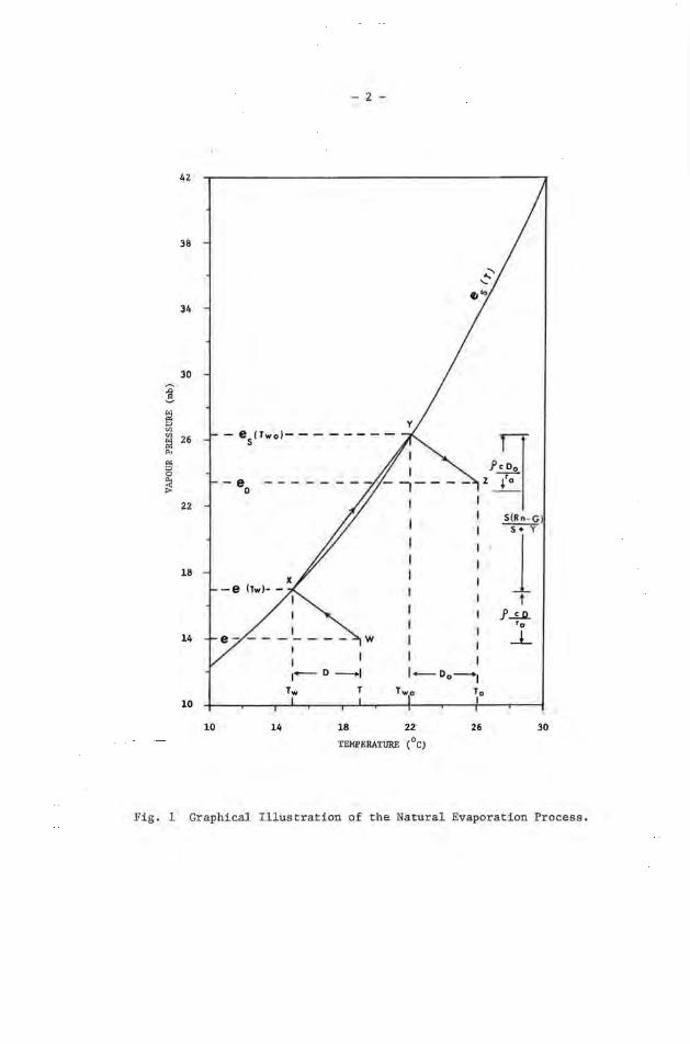
Fig. 1 Graphical Illustration of the Natural Evaporation Process.

- 3 -

evaporating surface. The derivation which follows and the graphical illustration

of the process (Fig. 1) are essentially the same as those presented by Monteith

(1965), but are included here for the specific purpose of explaining the

concept of equilibrium evapotranspiration.

The natural evaporation process, and the resulting energy exchanges,

are illustrated in Fig. 1. Evaporation of water into initially unsaturated

air (point W) may proceed until saturation occurs (point X). The heat required

for the conversion of the liquid water to vapour is provided by the sensible

heat contained by the air. The resulting decrease in the sensible heat content,

~QH' is represented by

P cD (1)

where p is the air density, c is the specific heat of air at constant pressure,

and D is the temperature decrease in the air, which in this case is equal to

the wet-bulb depression.

change heat with 1 cm2

of

3 If ra is the time required for 1 cm of air to ex-

the water surface, then the latent heat flux, LE1

, is

(2)

Evaporation may continue beyond this point only if there is an addition of heat

to the parcel of air. This will result in an increase in both the air

temperature, T, and the vapour pressure, e, with corresponding increases in the

sensible heat content, QH' and the latent heat content, QL' of the air. These

are related (Brunt, 1939) by

(3)

where y is the psychrometric constant (y = 0.66 mb °C-l ). Since the air is

saturated at point X, e may be replaced by the saturation value, es

' In this

case, small changes of vapour pressure and temperature are related by

S dT de s

(4)

where S is the slope of the saturation vapour pressure - temperature curve at

the current air temperature. Rearranging equation (3) and substituting es

for e,

- 4 -

(5)

and substituting equation (4) into (5) yields

(6)

Adding and subtra~ting S dQL on the right hand side of (6) and rearranging

terms gives

(7)

and hence

(8)

The term dQL for unit time is equal to the latent heat flux, LE2 , during the

saturated portion of the evaporation process. Also, (dQH + dQL) represents

the total heat gain by the parcel, and in a natural situation this heat would

be provided by the difference between the net radiation, Rn, and the soil heat

flux, G, so that

S(Rn - G) S + Y

(9)

The temperature and vapour pressure conditions in the air parcel might now be

represented by point Y in Fig. 1, which corresponds to the wet-bulb temperature

of the air at a natural evaporating surface. If the air at the surface was not

saturated, then its condition might be represented by point Z. To reach this

point from Y, latent heat must be released from the air at a rate given by

pcD o

r a

(10)

where Do is the wet-bulb depression in the air at the surface. The total

latent heat flux, LE, for the path W to Z is then the sum of the three comp­

onents, which may be written as

LE S(R - G)

n

S + y +

pc(D - D ) o

r a

(11)

- 5 -

This is the form of the combination model presented by Slatyer and McIlroy

(1961). In principle, S should be calculated at the mean of the wet-bulb

temperatures in the air and at the surface. However, temperatures at a natural

evapotranspiring surface are difficult to measure accurately, so an approximation

is required. As indicated in Fig. 1, the dry-bulb temperature of the overlying

air will usually be close to the mean wet-bulb temperature, and so it may be

used to calculate the value of S. This can be accomplished by using an

approximate solution for S which was presented by Dilley (1968). Incorporating

the assumption that T = (Tw + T )/2, S may be calculated as o w

S de

s dT

~ 25,029 exp

(T+237.30)2

l 7.269T

T+237.30 (12)

The formulation for LE presented in equation (11) is not practical

for general use due to the difficulty of measuring Do' but it is instructive

because it separates the basic energy sources. The first term on the right­

hand side represents the net amount of radiant energy directly expended on

evapotranspiration, while the second term represents the energy used from the

atmosphere for this purpose. It is the second term which is principally

responsible for evapotranspiration differences between surfaces of different

wetness. When a surface is wet or moist, the air close to it is saturated

(Do = 0). This is the potential evapotranspiration condition which is

considered in the Penman (1948) model. However when the water supply to the

surface is restricted, Do acquires a finite value and the actual evapotrans­

piration rate will be less than the potential. Recent combination model

developments by Monteith (1965), Tanner and Fuchs (1968), and Fuchs et al.

(1969) have in fact been attempts to eliminate Do in favour of other parameters

which may be more easily measured or estimated.

Slatyer and McIlroy (1961) considered the special and apparently

limited case when the two depressions are equal, thereby eliminating the

atmospheric term. This reduces equation (11) to

LE c S(Rn - G)

S + y (13)

In this case the evapotranspiration rate is simply a function of the available

radiant energy and the air temperature. The approach is essentially an energy

balance one, with the Bowen Ratio equal to y/S.

Monteith (1965) and Tanner and Fuchs (1968) have drawn attention to

the fact that equation (13) describes the evapotranspiration which would occur

- 6 -

in a saturated atmosphere. This is the simplest case in which the depressions

are equal, because both are equal to zero. However it is possible that the

depressions might have finite values and still be equal or nearly equal, in

which case equation (13) would remain valid or stand as a good approximation.

5latyer and McIlroy (1961) considered that equality of the depressions occurred

when the surface and the overlying air had adjusted to one another, and so

they suggested that the conditions described by equation (13) should be referred

to as "equilibrium" evapotranspiration.

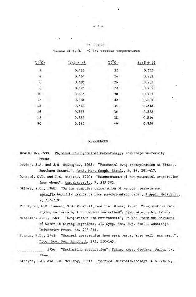
The equilibrium model is appealing because of its simplicity. The

parameters Rn, G, and T are easily measured or estimated and the weighting

factor 5/(5 + y) may be calculated as an integral part of a computer programme

or it can be determined from a table (see Table One). Use of the model is

warranted, however, only when D = Do' This situation is not likely to occur

either when the surface is wet (D»Do

) or when it is very dry (D«Do)' It

seems probable that there must be a middle range of moderately dry surface

conditions when D ~Do and the equilibrium estimates will closely approximate

the actual evapotranspiration rate.

The accuracy of the equilibrium model and the moisture limits within

which it may be applied are currently under investigation by the author, and

the results to date are extremely encouraging. The model is only an approximation

of the actual evapotranspiration process, so a certain degree of error must

be expected in the estimates. Consequently the problem has essentially become

one of defining those limi.ts ,.,ithin which the estimates are reasonably accurate.

Maximum errors of +10 percent of daily evapotranspiration would probably be

acceptable for most potential hydrological and agricultural applications

(Penman, 1956 ; Tanner, 1960). There are strong indications that the

equilibrium model satisfies these demands for quite a wide range of moderately

dry surface conditions when the actual evapotranspiration rate is less than the

"potential" rate. In a recent study, Denmead and McIlroy (1970) compared hourly

values of equilibrium evapotranspiration with measured values. The data

exhibited a moderate degree of scatte,: and the model p"roduced underestimates

at high evapotranspiration rates. The authors suggested that the equilibrium

rate is probably approached closely on only a few occasions, but they also

expected that departures from the actual rate would rarely be extreme. These

results and conclusions provide further evidence of the potential capabilities

of the equilibrium model, but they clearly indicate the necessity of defining

the limits within which its use is justified. If these can be established,

the equilibrium model may prove to be the first operational method of accurately

predicting short-term evapotranspiration losses for drying surfaces.

- 7 -

TABLE ONE

Values of S/(S + y) for various temperatures

T(oC) S/(S + X) I.L£l S/(S + r)

2 0.433 22 0.709

4 0.464 24 0.731

6 0.495 26 0.751

8 0.525 28 0.769

10 O. "555 30 0.787

12 0.584 32 0.803

14 0.611 34 0.818

16 0.638 36 ~.832

18 0.663 38 0.844

20 0.687 40 0.856

REFERENCES

Brunt, D., 1939: Physical and Dynamical Meteorology, Cambridge University

Press.

Davies, J.A. and J.H. McCaughey, 1968: "Potential evapotranspiration at Simcoe,

Southern Ontario", Arch. Met. Geoph. Biokl., B, 16, 391-417.

Denmead, O.T. and I.C. McIlroy, 1970: "Measurements of non-potential evaporation

from wheat", Agr.Meteorol., 7, 285-302.

Dilley, A.C., 1968: "On the computer calculation of vapour pressure and

specific humidity gradients from psychrometric data", J . Appl. Meteorol..

7, 717-719.

Fuchs, M., C.B. Tanner, G.W. Thurtell, and T.A. Black, 1969: "Evaporation from

drying surfaces by the combination method", Agron.Jour., 61, 22-26.

Monteith, J.L., 1965: "Evaporation and environment", In The State and Movement

of Water in Living Organisms, XIX Symp. Soc. Exp. Biol., Cambridge

University Press, pp. 205-234.

Penman, H.L., 1948: "Natural evaporation from open water, bare soil, and grass",

Proc. Roy. Soc. London A, 193, 120-145.

1956: "Estimating evaporation", Trans. Amer. Geophys. Union, 37,

43-46.

Slatyer, R.O. and I.C. McIlroy, 1961: Practical Microc1imatology C.S.I.R.O.,

- 8 -

Melbourne, Australia.

Sziicz, G. and I.F. Long, 1969: "Sourface resistance of crop canopies",

Water Resources Res., 5, 622-633.

Tanner, C.B., 1960: "A simple aero-heat budget method for determining daily

evapotranspiration", Transactions, 7th Internat.Cong. Soil Sci.

Madison, Wisconsin. and M. Fuchs, 1968: "Evaporation from unsaturated surfaces: a

generalized combination method", J.Geoph.Res., 73, 1299-1304 .

1. Introduction

- 9 -

SOIL HEAT FLUX DIVERGENCE IN A

DEVELOPING CORN CROP

by

R.G. Wilson and J.H. McCaughey*

The energy balance framework is frequently used to assess evapo­

transpiration losses from vegetated surfaces. This approach is taken in Bowen

Ratio measurements and in combination model predictions of the water vapour

flux. The balance of energy can be written as

Rn - G LE + H (1)

where Rn is the net radiation, G is the soil heat flux, LE is the latent heat

flux, and H is the sensible heat flux. An investigator using either the Bowen

Ratio or the combination model approach must determine the quantity (Rn - G).

Rn is clearly the most important term since it represents the total energy in­

put in the balance. On the other hand, G is frequently the least important

of the three energy dissipation terms in equation (1). Measurements have

indicated that it usually represents only 5 to 10 percent of Rn for completely

vegetated surfaces (Tanner and Pelton, 1960; Sellers, 1965, p. 111; Davies

and McCaughey, 1968; Wilson, 1970). This proportion generally increases with

a greater exposure of bare soil; for example, Decker (1959) found that soil

heat flux under short corn plants represented 15 percent of Rn. The importance

of this amount of energy should not be overlooked. Good evapotranspiring

conditions are indicated when the Bowen Ratio (S H/LE) has a value of

S = 0.2. In a situation where S = 0.2 and G = 0.15 Rn, then H 0.14 Rn. Thus,

the fluxes of soil heat and sensible heat are approximately equal. Under these

or similar conditions, G should be measured with the same precision as the other

energy terms. Unfortunately many soil heat flux measurements have been made

* R.G. Wilson is Lecturer in Climatology at McGill University. J. H. McCaugheyis a doctoral candidate in Climatology at McMaster University.

- 10 -

without proper consideration of the accuracy of the determination.

The flux of heat into a soil is given by

G - A dT (2) az

Where A is the thermal conductivity of the soil and ClT/ClZ is the vertical

gradient of soil temperature between the surface and depth Z. Equation (2) is

infrequently used in field investigations because of the difficulties experienced

in measuring A and ClT/ aZ near the soil surface. These problems are eliminated

by the use of heat flux transducers. Frequently the transducers are placed about

1 or 2 cm below the surface, and the recorded flux is assumed to be equal to the

flux occurring at the surface. However, this procedure may introduce significant

errors in the estimates of G. A flux plate should not be installed so close

to the surface because it interferes with moisture flow and thereby creates

sampling dissimilarities. Another sampling problem may also be created by

surface heterogeneities. These problems may be overcome by placing the plate

deeper in the soil, but then errors may be caused by soil heat flux divergence

between the plate and the soil surface.

As a result of these considerations, it is usually recognized that

the most practical and accurate method of determining the heat flux at the

surface involves measuring the flux at a depth of 5 to 10 om and then accounting

for the heat flux divergence between the plate and the surface {van Wijk, 1965;

Sellers, 1965, p. 131; Fuchs and Tanner, 1968). In this case the surface flux,

Go is given by ~

G o

GZ

+ C fiT Z fi t

(3)

where Gz is the flux at depth Z and fiG is the heat flux divergence between

depth Z and the surface, C is the heat capacity of the soil between depth Z

and the surface, and fiT/fit is the change of the mean temperature of the layer

per unit time.

The heat capacity can be written as

C (4)

where Cm' Co' Cw

and Ca are the heat capacities of mineral and organic matter,

water, and air, respectively , and Xm, Xo ' ~,and Xa are the corresponding

volume fractions of each constituent. The heat capacity of air is so small

compared to the others that the term CaXa may be safely neglected. De Vries

'\:

- 11 -

(1963) suggested average values of C = 0.46 and C -3 0 -1 m 0

cal cm C, so that equation (4) reduces to

0.60, whereas Cw 1.0

C z 0.46 ~ + 0.60 Xo + Xw (5)

The values of X and m

Xo will remain constant for a given location, so it

is necessary to routinely measure only x . w

2. Experimental

Soil heat flux was measured in a series of energy balance investigations

at the Simcoe Horticultural Research Station in Southern Ontario during the

summer of 1969. The research programs have been described earlier by Davies,

Rouse, and Oke (1970). All measurements were conducted in a large field of sweet

corn (Zea Mays: horticultural variety Seneca Chief) which was planted in 1m

rows oriented in a NW - SE direction (Fig. la). The growth curve during the

study period in July and August is shown in Fig. lb.

The soil heat flux instrumental array (Fig. la) comprised three soil

heat flux plates and a number of thermocouples. The soil heat flux plates

(Middleton and Pty Ltd.) were installed at a depth of 5 cm and were connected

in series to give a spatial average of the flux at that depth. The mean soil

temperature between the surface and 5 cm depth was measured with thermocouples

connected in series. Individual junctions were mounted on 3/4" wooden dowels

and 15 cm of thermocouple wire were wrapped around the dowels at each measurement

level to eliminate conduction errors. The mounted thermocouples were placed at

depths of 0.5, 1.5, 2.5, 3.5, and 5.0 cm. The common reference junction was

installed at a depth of 1.5 m and the temperature at that depth was monitored

by a separate thermocouple which was referenced to an ice-water bath. The

signal from the flux plates was continuously recorded on a Honeywell

Electronik 194 strip chart recorder and was integrated with a planimeter to

give hourly values of G5

• All temperature signals were measured and recorded

by a Solartron data system, and hourly values of ~T/~t were subsequently

determined.

The heat capacity of the surface soil (Caledon sandy loam) was

calculated from equation (5). Mean values of x = 0.459 and m Xo = 0.024

were determined by "loss on ignition" treatments of five soil samples, thereby

reducing equation (5) to

C = 0.225 + x . w

D

Crop Height (em)

200

150

100

50

o

X (1. Scm)

X (0.5cm)

I COHN

<:-

SOIL HEAT FLUX RATE AT 5 . Ocm

10 15

JULY

- 12 -

Cl X (2.5cm)

X (5.0cm)

(3.5cm)

X THERMO JUNCTION

20 25 30 1

AUGUST

Fig.l Energy Balance Investigations at Simcoe: (a) upper plan of field site and instruments;

10

(b) lo~er - growth curve of corn crop during July and August.

- 13 -

Volumetric soil moisture content was determined by gravimetric analysis of ten

soil samples each day. The moisture content of each sample was calculated as

x = w W D

x (7)

where W is the weight of water in the sample, D is the dry weight of the sample,

and p is the mean dry density of the soil. A total of 300 density samples s -3

produced a mean value of Ps = 1.2S g cm The average value of Xw from the

ten samples was then used to calculate C from equation (6), which in turn was

used to calculate hourly values of soil heat flux divergence and Go from

equation (3).

3. Results

Soil heat flux divergence was found to contribute significantly to

Go on both an hourly and a daily basis. Hourly values of Rn, GS

' and Go for two

sunny days, (July 6 and August 11), are plotted in Fig. 2a. On both days Go was

considerably larger than GS

in the morning hours, with a reversal of this situation

occurring in the afternoon. The reversal (GS

> Go) continued throughout the

afternoon of August 11 but was interrupted in the late afternoon of July 6.

Hourly patterns such as these occurred persistently throughout the study period

and can be related to the variations of soil heating and cooling. Surface soil

temperatures increased rapidly in the morning hours due to solar heating, thereby

producing large positive values of soil heat flux divergence. In the early

afternoon hours the soil surface cooled and the divergence became negative. The

interruption of this situation on July 6 was a characteristic of sunny days during

the first two weeks in July. The corn plants did not provide a complete ground

cover at that time, so the soil intercepted direct solar radiation in the late

afternoon when the sun shone down the rows. A short period of soil heating

resulted, causing a condition of positive divergence. After the middle of July

the leaves shaded the soil throughout the day and the divergence tended to

remain negative during the afternoon hours.

The effect of the developing crop is also apparent in the trends of

daily values of the ratios Go/Rn and GS/Rn (Fig. 2b). There was an overall

tendency for values of both ratios to decrease as the crop grew higher, with

sharp daily variations occurring in periods of rains. For the entire study

period, average values of the ratios were Go/Rn = 0.083 and GS/Rn = 0.049.

Thus, even on an average daily basis, neglect of the flux divergence would have

- 14 -

ly.min -1

O.8,----------------------r---------------------r ly.min -1

0.8

0.6

0.4

0.2

0.0

08 12 16 20

Ratio

AUGUST 11

-I

I 1

1 I

I I

I I

", I " ... ,' ,,,,",, l-::: .. ···· .. ' " ... ' .. ','':''':': ',.:: ~ :.:"

08 12 16

0.6

0.4

0.2

0.0

20 DST

0.2,--------------------------------------------------------,

0.1

0.0

-0.1 10 15 20 25 30 1

JULY

Fig.2 Net Radiation and Soil Heat Flux at Simcoe: (a) upper - hourly values on two days;

10

AUGUST

(b) lower - heat flux/net radiation ratios, July and August.

- 15 -

produced a mean error of nearly 60% in the soil heat flux measurements. This

error would have been larger at the beginning of the study period and smaller

at the end because the magnitude of the divergence decreased over that period.

It was particularly important to measure the divergence during individual

hourly periods, as was apparent in Fig. 2a. As an example, the computed

evapotranspiration between 0900 hand 1000 h on July 6 would have been over­

estimated by 27 percent if the divergence had been neglected. Although this

figure was smaller for the comparable period on August 11 , it is clear that

the divergence was still significant even when the crop was fully develo;>ed.

TABLE ONE

Regression Analysis for Daily Totals of G (energy values in cal cm-2day-l, crop height in °cm)

Correlation Standard Regression Eguation Coefficient Error

A. G 8.0 + 1.19 G5

0.88 7.0 0

B. G -10.5 + 1.00G5

+ 0.07Rn 0.91 6.3 0

C. "G -4.5 + O.95G5 + 0.07Rn

'" - 0.07h 0.94 5.1

A linear regression analysis (Table One) indicates that daily values

of Go may be estimated with reasonable accuracy from Rn, G5

, and crop height h.

When all three variables are used together the standard error is only -2 -1

5.1 cal cm day The error was not significantly improved when soil moisture

content was included in the regression.

4. Conclusions

Soil heat flux divergence between the 5 cm depth and the soil surface

involved significant quantities of energy for both hourly and daily periods.

Consequently, there would have been large errors in the evapotranspiration

estimates if the divergence had not been taken into account, even when the crop

was fully developed.

A change in the instrumental array would be recommended for future

studies. Rapid soil temperature fluctuations were occasionally observed during

individual hourly periods at the beginning of July. These were probably caused

by the presence of sunflecks near one or more of the thermocouple junctions.

This problem might be eliminated by placing two or three junctions at each

- 16 -

deptn, so that the measured temperature change would then be more representative

of the average situation. The measurement technique used in this study and

the recommended improvement are slightly troublesome. However our experience

indicates that considerably more attention should be given to soil heat flux

measurements than has generally been the case in the past.

REFERENCES

Davies, J.A. and J.H. McCaughey, 1968: "Potential evapotranspiration at

Simcoe, Southern Ontario", Arch. Met. Geoph. Biokl., Ser. B,

16, 391-417.

Decker, W. 1., 1959: "Variations in the net exchange of radiation from

vegetation of different heights", J. Geophys. Res., 64, 1617-1619.

Fuchs, M. and C.B. Tanner, 1968: "Calibration and field test of soil heat

flux plates", Soil Sci. Soc. Amer. Proc., 32, 326-328.

Sellers, W.D., 1965: Physical Climatology, University of Chicago Press.

Tanner, C.B. and W.L. Pelton, 1960: "Energy balance data, Hancock, Wis.,

"University of Wisconsin Soil Bull, 2.

van Wijk, W.R., 1965: "Soil microclimate, its creation, observation and

modification", Agricultural Meteorology, Met. Mono. 6, 59-73.

Wilson, R.G., 1970: "Topographic influences on a forest microclimate",

McGill University Climatological Research Series 5.

- 17 -

NOTES SUR UNE METHODE DESCRIPTIVE DES TYPES DE TEMPS(l)

par

André Hufty*

LA METHODE EMPLOYEE

Il existe de nombreuses méthodes d'analyse des éléments du climat.

Elles diffèrent entre elles par la façon dont les éléments sont groupés et

par les périodes choisies.

J'ai comparé 8 stations climatiques pendant 6 ans à partir des

fr€quences journalières de combinaisons d'éléments du temps, ou fréquences

de types de temps. Les éléments qui entrent dans ces regroupements sont les

suivants: températures maximales et minimales et indices d'aggravation du

temps ("bad weather index") basés sur la durée d'ensoleillement et les

précipitations. Chaque jour est ainsi gratifié de deux symboles: le premier,

de A à l est fonction de la température, le second dépend de l'état du temps

(voir légende, p. 21).

Comme on a neuf classes de température et cinq classes d'aggravation

du temps, on obtient 45 possibilités pour chaque jour. Ce nombre de types

de temps est tr~p élevé et il a été réduit, compte tenu des résultats obtenus,

à 15, chiffre plus maniable (voir légende, p.21 ).

QUELQUES RESULTATS OBTENUS

Pour simplifier les analyses, je vais comparer d'abord les seuls

groupements thermiques, ensuite les seuls indices d'aggravation du temps et

enfin les résultats complets mais seulement pour quelques stations afin de

donner un aperçu de la methode utilisée.

(1)

* Le manuscrit complet est déposé à la revue "The Canadian geographer".

André Hufty est professeur de climatologie à l'Université Laval.

Types de

temps

Saisons:

Indices 2 et 3

Québec

CapIan

Indices 5 et 6

Québec

CapIan

J

57

59

- 18 -

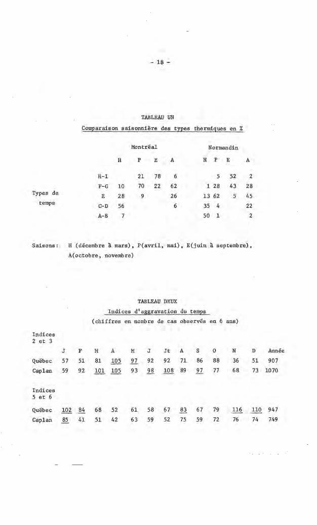
TABLEAU UN

Comparaison saisonnière des types thermiques en %

Montréal Normandin

H P E A H P E A

H-I 21 78 6 5 52 2

F-G 10 70 22 62 1 28 43 28

E 28 9 26 13 62 5 45

C-D 56 6 35 4 22

A-B 7 50 1 2

H (décembre à mars), P(avri1, mai), E(juin à septembre),

A(octobre, novembre)

TABLEAU DEUX

Indices d'aggravation du ternEs

(chiffres en nombre de cas observés en 6 ans)

F M A M J Jt A S 0 N D

51 81 105 97 92 92 71 86 88 36 51

92 101 105 93 98 108 89 97 77 68 73

102 84 68 52 61 58 67 83 67 79 116 110

85 41 51 42 63 59 52 75 59 72 76 74

Année

907

1070

947

749

- 19 -

(1) Groupements thermigues

L'analyse du Tableau Un, va nous permettre de comparer deux stations

fort différentes.

D'après ce tableau, qui regroupe les deux stations les plus contrastées,

on constate qu'il y a un décalage d'une catégorie d'une ville à l'autre: en

hiver, les temps froids sont nombreux à Montréal mais la température dépasse

le point de gel plus du tiers des journées et ne s'abaisse que très rarement

en dessous de -30oC (-230 F); à Normandin par contre, les temps très froids

sont la règle, avec deux dizièmes des nuits inférieures à -30oC.

Les gelées nocturnes disparaissent au centre de Montréal au cours du

mois d'avril mais persistent deux jours sur trois dans le centre de la

province. En été, il peut faire très chaud partout, mais ces fortes chaleurs

sont les plus fréquentes le long de la plaine du Saint-Laurent.

Le mois d'octobre est encore beau à Montréal mais il gèle déjà plus

d'un jour sur deux à Normandin (contre un sur dix à Montréal). L'arrivée de

l'hiver dans les deux villes est décalée de presque 6 semaines.

(2) Groupements par indices d'aggravation du~ (voir Tableau Deux)

Dans l'ensemble du Québec, la fréquence des temps clairs et secs passe

par un maximum de mars à mai, descend lentement jusqu'au mois d'août, pour

remonter temporairement en septembre, avant la chute qui conduit au minimum

de novembre, suivie elle-même d'une remontée assez rapide jusqu'en mars.

En hiver, Québec est moins ensoleillé que CapIan; les deux stations

se ressemblent à la fin du printemps. Au cours de l'été les temps clairs et

ensoleillés sont nombreux partout mais surtout à CapIan, même en août. La

chute de novembre est moins forte à CapIan qu'à Québec.

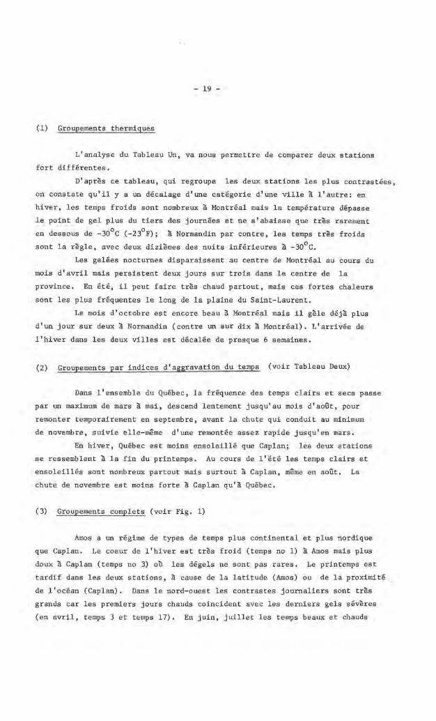
(3) Groupements complets (voir Fig. 1)

Amos a un régime de types de temps plus continental et plus nordique

que CapIan. Le coeur de l'hiver est très froid (temps no 1) à Arnos mais plus

doux à CapIan (temps no 3) où les dégels ne sont pas rares. Le printemps est

tardif dans les deux stations, à cause de la latitude (Arnos) ou de la proximité

de l'océan (CapIan). Dans le nord-ouest les contrastes journaliers sont très

grands car les premiers jours chauds coincident avec les derniers gels sévères

(en avril, temps 3 et temps 17). En juin, juillet les temps beaux et chauds

100%

50%

K A

GEL [ CONTINU

1 1 1 ,

1

1 • 1 5

3 : _ _____ i _

1 6 - 7

GI':L- [ DEGEL

1 8 1 9 110

POU ni: [ GEL

1 12 - 13

Il - ' 04 , ----,-1 15 1 16

1 1 17 1 18 1 19

1

"

- 20 -

I«lI<IREAL

11

" -"- , "- /

, ~

---~ /

AKOS

CLASSE J-: Te.pli ensoleillé, sans pn!clpltationsj il gèle couee la journée, avec un Ininil!lul!I sup~l"ieur );j _4° F

l:l .. flSSt: 16: TeOlps crès couvert et pluvieux. Il ne gèle pas et la tempérll[Ure llI8.xlll1.ale est in[érleure à 68° F.

Fig. l Types de Temp: Montréal et Amos .

gel continu

passage gel-dégel

pas de gel

- 21 -

LEGENDE DES TYPES DE TEMPS

Catégories de température (oF):

minimum journalier maximum journalier

A polaire ou -41 31 glacial -23 à -40 (-40°C) 31

B très froid -5 à -22 (-30°C) 31

C froid 13 à -4 (-20°C) 31

D frais 31 à 14 (-lOoC) 31

E frisquet 32 et maximum 32

F tempéré 33 de 33 à 50 (lOoC)

G doux 33 51 à 68 (20oC)

H chaud 33 69 à 86 (30oC)

l très chaud 33 87 à 95 (350 C) ou torride 33 96

Indices d'aggravation du temps: additionner les chiffres ci­

dessus pour obtenir un indice journalier variant de 2 (temps

ensoleillé et sec) à 6 (temps couvert avec précipitations).

Les indices 3 à 5 indiquent un temps variable avec augmentation

des nuages et des précipitations.

(1) catégories

1. nulles 2. traces ou 0.01 pouces d'eau tombée 3. 0.02 pouces ou plus

(II) catégories d'ensoleillement, basées sur les rapports d'ensoleillement:

1. plus de 6/10 de l'ensoleillement possible 2. de 2 à 6/10 de l'ensoleillement possible 3. moins de 2/10 de l'ensoleillement possible

Remarque: Utiliser les valeurs suivantes, des rapports d'ensoleillement en heures et dizièmes d'heure extraites de l'annuaire du Québec.

J F M A M J Jt A S 0 N D

6/10 5.3 6.0 7.1 8.1 9.1 9.5 9.2 8.7 7.7 6.6 5.7 5.1

2/10: 1.7 2.0 2.4 2.7 3.0 3.1 3.0 2.8 2.6 2.2 1.9 .17

- 22 -

sont plus fréquents à Amos et les jours ensoleillés restent souvent frais à

CapIan (temps 11-14). Cependant, dans le nord-ouest, on observe plus un

grand nombre de jours à ciel couvert et pluvieux (temps 15, 16, 18, 19). En

août et en septembre, les temps clairs se refroidissent mais il gèle rarement

près de la mer et la fin de l'été y est très ensoleillé. Dans le nord-ouest,

les temps doux et très couverts sont très nombreux (temps 15-16) et les

contrastes journaliers sont violents en septembre qui est déjà un mois

d'automne. De septembre à octobre la diversité des types de temps augmente.

Le froid s'accentue et la nébulosité devient plus grande: ces deux effets vont

s'amplifier en novembre où le type de temps le plus caractéristique est le

numéro 10, c'est-à-dire un jour sombre avec pluies diurnes et neiges nocturnes.

Les gelées nocturnes passent de 0 à 100% du début septembre à la fin novembre

à Amos mais à CapIan, même en octobre les temps clairs ont peu de gelées et

des faibles amplitudes de température (temps no Il ou 14).

Pour donner une idée meilleure de la méthode, il faudrait comparer

plus de stations, avec des chiffres précis pour les différentes catégories.

Cependant cette analyse sommaire permet de faire ressortir la continentalité

d'Amos (plus de temps clairs et froids en hiver, plus de temps chauds en été),

et l'effet de sa position en latitude (températures plus basses, été plus per­

turbé à cause des dépressions cycloniques décalées vers le nord à cette saison).

L'influence maritime se fait sentir à CapIan par une atténuation des contrastes

entre l'hiver et l'été et par un décalage des saisons intermédiaires (printemps

tardif, automne très doux).

CONCLUSION

Cette méthode est simple à employer (70 étudiants de licence en

géographie ont aidé au dépouillement des données journalières), assez laborieuse

mais on peut faire calculer les fréquences par un ordinateur. La méthode

permet une bonne description des climats à partir des situations journalières

qui sont plus significatives que les moyennes dans les pays tempérés ou

l'irrégularité du temps est très forte. Elle peut être améliorée facilement

en définissant autrement les classes: c'est ainsi qu'en hiver on pourrait

tenir compte du vent, classer les jours par indices de refroidissement (wind

chilI), mettre à part les jours de tempêtes de neige. De même en été, il

faudrait tenir compte de l'humidité relative et du bilan d'eau. En somme,

cette méthode est ouverte à quantité d'ajustements qui pourraient donner des

résultats intéressants en climatologie appliquée. La discussion le fera grandir.

- 23 -

RESEARCH REPORT

Since the publication of the last issue of the Bulletin daily totals of solar and net radiation for Mont St. Hilaire have been compiled for the period 1966-69. Preliminary analysis of these totals has been concerned with three topics: (1) comparative measurements of solar radiation with three different instruments; (2) variability of surface albedo during the year; and (3) linear relationships between solar and net radiation.

Analysis for part (1) indicates that both the Belfort bimetallic actinograph and the Yellot Mark IV Integrating Sol-A-Meter have a non-linear response at low radiation values. However, when they have been calibrated against a control instrument (in this case a Kipp and Zonen solarimeter) their accuracy seems reasonable for many purposes. In this case the standard errors of prediction were found to be about 10 percent for daily values and 5 percent for weekly totals.

The average albedo of the short grass cover during the summer of 1968 was 0.25 with a standard deviation of 0.03. A greater variability was found for snow which, for the winter months of 1968, had a mean of 0.85 and a standard deviation of 0.14.

Linear relationships between solar and net radiation have been determined for daily and weekly totals for both grass and snow. Correlation coefficients average about 0.90 and standard errors of prediction are approximately 30-40 langleys per day. These results clearly indicate the feasibility of using this technique for daily or weekly periods, rather than monthly periods as has been common in the literature.

Within the field of urban climatology, a pilot study has been started to examine certain aspects of the climate of Montreal in relation to human physiological stresses. The study aims to sample conditions within the urban area by taking observations at different places during the different seasons of the year, and applying the results to an examination of physiological stresses through the use of standard formulae.

With this end in view, twelve sites were selected to represent the city area. They were chqsen along an east-west axis from the St. Lawrence river to van Horne street on the other side of Mt. Royal. Thus, the sample embraces the tourist area of Old Montreal, the city's business district in the vicinity of St. James Street, the commercial core of the downtown area, and some of the' residential areas well within the urban region. The actual positions chosen also sample different kinds of urban structure and, for the most part, are concerned with places where large numbers of people are found in the streets. Since the study aims to relate the city climate to people in the street, the choice of such sites was deemed important as was the choice of the time of observation: 1200-1400 hours, which covers the lunch-hour for most people in the downtown area. This time also is a period of the day when conditions of temperature, humidity, and radiation tend to change least, so that it was possible to obtain some impression of variation from place to place within the city.

- 24 -

Observations of wind speed and humidity were made by means of a car traverse along the traverse route. Sensitive cup anemometer (C.F. Casella & Co.) were used for the former, and an Assmann ventilated hygrometer for the latter. Both were mounted on a car in positions which calibration showed too be minimally influenced by the effects of the vehicle itself. The police Department of the city co-operated by granting a special permit for the vehicle to be parked whenever and wherever necessary for the observations. By selecting "no parking areas" for the actual site of observations it was possible to ensure that each observation spot was identical for every traverse. Observations began at the end of July, 1970, and continued at selected intervals through February, 1971. The selection of observation periods was made as far as possible to sample the weather of different seasons. Each observation period lasted 7-10 days to cover a full weather cycle, and the observations were made each day during the period in question.

The reslting data were incorporated in appropriate formulae such as the comfort index or the wind chill factor. It had been impractical to take radiation observations during the traverses. However, at every observation ~ note was made as to whether the observation was being made in shade or in sunshine. Sky-line measurements of each site were also used to prepare sky­line profiles around each site. These enabled an evaluation of radiation for each site to be made by obtaining the hourly data of global and sky-diffuse radiation observed at Jean Brebeuf College for the Federal Meteorological Service, and adjusting the figures for the sky-line conditions at each observation site. Thus it has proved practical to include in the analysis formulae which incorporate the radiative heat load on the human body.

Analyses of all these data are currently being undertaken and will be the subject of later reports in this Bulletin and elsewhere.

B. J. Garnier Professor of Climatology McGill University

- 25 -

NEWS AND COMMENTS ----

Messrs G. D. Mackay & B. F. Findlay of the Department of Transport (Meteorological Branch) visited McGill University in October and participated in a graduate seminar devoted to discussing two aspects of urban climatology: a pilot study of human comfort values in the city of Montreal, and a project to evaluate the differences in the radiation balance between Montreal and the adjacent countryside.

The second annual reunion of Friends of Climatology was held March 12-13. The hosts for the occasion were members of the Department of Geography at MacMaster University. Social activities and a period of discussion which covered many practical problems of climatological research 1n Canada, were followed by short talks by Professors F.K. Hare and H. Lettau, and a keynote address on East African Rainfall by Professor Thompson of Brock University.

Professor B. J. Garnier was an invited lecturer to the WMO 'Seminar on Agricultura! Meteoro!ogy held in Barbados in November, 1970. His topic of discussion was the organisation of Observation Networks in Agrometeorology.

There have been some recent modifications in the climatological courses being offered in the Department of Geography at McGi!l University. In the past there have been two full undergraduate courses at 3rd and 4th year levels respectively. These have now been divided into four half-courses, each lasting one semester. The four half- courses now available are: (a) Climatic Environments; (b) Ecological & Physiological Climatology;(c) Urban Climatic Environments; and (d) Agro & Hydro-climatology. "The purpose of this change is to widen the effective offering for students requiring some climatology especially applied climatology, but who do not intend to specialize in the field. Slight changes in prerequisites will make it possible for those who obtain basic climatology outside of geography, e.g. through meteorology, to enter the courses without going through the courses which comprise the standard prerequisites.

No.1

No . 2

No.3

No.4

No.5

No . 6

McGill University

Department of Geography

CLIMATOLOGICAL RESEARCH SERIES ---

Two Studies in Barbadian Climatology, by W.R. Rouse and David Watts, 65 pp., July 1966, price $ 6 . 50.

Weather Conditions in Nigeria, by B.J . Garnier, 163 pp., March 1967 -out of print. Climate of the Rupununi Savannas - A study in Ecological Climatology, by David B. Frost, 92 pp., December 1967 - out of pri nt.

Temperature Variability and Synoptic Cold Fronts in the Winter Climate of Mexico, by J.B.Hill, 71 pp . , February 1969, price $ 7.50.

Topographic Influences on a Forest Microclimate. by R.G.Wilson, 109 pp .• September 1970, price $ 10.00

Estimating the Topographic Variations of Short-Wave Radiation Income: The Example of Barbados, by B.J.Garnier and Atsumu Ohmura, 66 pp., December 1969, price $ 7.50

Prices of RESEARCH SERIES vary, but subscribers to the BULLETIN are entitled to a 50% reduction on the published price, provided they hold or held a current subscription for the "year in which the relevant number of the Research Series appears.

Send orders and enquiries to:

Department o"f Geography (Climatology), McGill University, P.D.Box 6070, Montreal lOl.P.Q. Canada.