mceliece using quasi dyadic goppa codes - cdc · pdf filein 1948 claude shannon founded...
TRANSCRIPT

Implementation of McEliece using quasi-dyadic Goppa codes
1

Part I
StatementI hereby declare that the work presented in this thesis is my own work and that to the best of my knowledgeit is original except where indicated by references to other authors.
Gerhard Hoffmann, Darmstadt, April 25, 2011
2

Contents
I Statement 2
II Acknowledgements 6
III Introduction 7
IV The Algebraic Setup 8
1 Finite fields 8
2 Linear codes 92.1 Encoding messages. . . . . . . . . . . . . . . . . . . . . . . . . . . . . . . . . . . . . . . 102.2 Decoding messages. . . . . . . . . . . . . . . . . . . . . . . . . . . . . . . . . . . . . . . 122.3 Equivalence of codes and information sets. . . . . . . . . . . . . . . . . . . . . . . . . . 152.4 Generalized Reed Solomon codes. . . . . . . . . . . . . . . . . . . . . . . . . . . . . . . 16
2.4.1 Alternant codes . . . . . . . . . . . . . . . . . . . . . . . . . . . . . . . . . . . .. 212.4.2 Goppa codes . . . . . . . . . . . . . . . . . . . . . . . . . . . . . . . . . . . . . .21
2.4.2.1 Parity check matrix of a Goppa code. . . . . . . . . . . . . . . . . . . . . 222.4.3 Binary Goppa codes . . . . . . . . . . . . . . . . . . . . . . . . . . . . . . . . .. 252.4.4 Examples for binary Goppa codes . . . . . . . . . . . . . . . . . . . . . . . .. . . 27
2.4.4.1 Example . . . . . . . . . . . . . . . . . . . . . . . . . . . . . . . . . . . 272.4.4.2 Example . . . . . . . . . . . . . . . . . . . . . . . . . . . . . . . . . . . 28
2.4.5 Parity check matrix generated byg(X)2 in case of a binary, separable Goppa codes . 282.4.6 Parity check matrix generated byg(X)2 in Tzeng-Zimmermann form . . . . . . . . 292.4.7 Goppa codes in Cauchy and dyadic form . . . . . . . . . . . . . . . . . . .. . . . 302.4.8 The fast Walsh-Hadamard transform and the dyadic convolution . . .. . . . . . . . 31
V Code-based cryptosystems 34
3 The classical McEliece cryptosystem 343.1 Setup . . . . . . . . . . . . . . . . . . . . . . . . . . . . . . . . . . . . . . . . . . . . .. 343.2 Encryption . . . . . . . . . . . . . . . . . . . . . . . . . . . . . . . . . . . . . . . . .. . . 343.3 Decryption . . . . . . . . . . . . . . . . . . . . . . . . . . . . . . . . . . . . . . . . .. . 34
4 A modern McEliece cryptosystem 354.1 Setup . . . . . . . . . . . . . . . . . . . . . . . . . . . . . . . . . . . . . . . . . . . . .. 354.2 Encryption . . . . . . . . . . . . . . . . . . . . . . . . . . . . . . . . . . . . . . . . .. . . 354.3 Decryption . . . . . . . . . . . . . . . . . . . . . . . . . . . . . . . . . . . . . . . . .. . 35
3

5 McEliece based on binary quasi-dyadic codes 365.1 System parameters . . . . . . . . . . . . . . . . . . . . . . . . . . . . . . . . . . . .. . . 36
5.1.1 Generating the public and private keys . . . . . . . . . . . . . . . . . . . . .. . . . 365.1.2 Generating the public generator matrix . . . . . . . . . . . . . . . . . . . . . . .. 375.1.3 Generating a private parity check matrix . . . . . . . . . . . . . . . . . . . . .. . . 37
5.2 The encryption step . . . . . . . . . . . . . . . . . . . . . . . . . . . . . . . . . . .. . . . 395.3 The decryption step . . . . . . . . . . . . . . . . . . . . . . . . . . . . . . . . . . .. . . . 39
5.3.1 The setup . . . . . . . . . . . . . . . . . . . . . . . . . . . . . . . . . . . . . . . . 395.3.2 Solving the key equation using the Euclidean algorithm . . . . . . . . . . . . .. . . 415.3.3 Finding the roots of the error locator polynomial . . . . . . . . . . . . . . . .. . . 42
VI Algebraic attacks against quasi-dyadic McEliece 43
VII Implementation 44
6 Finite field implementation 446.1 Initialize the field . . . . . . . . . . . . . . . . . . . . . . . . . . . . . . . . . . . . . . .. 466.2 Release the field tables. . . . . . . . . . . . . . . . . . . . . . . . . . . . . . . . . .. . . . 476.3 Initialize the exponential table . . . . . . . . . . . . . . . . . . . . . . . . . . . . . .. . . 476.4 Initialize the logarithm table . . . . . . . . . . . . . . . . . . . . . . . . . . . . . . . . .. 486.5 Powers of field elements . . . . . . . . . . . . . . . . . . . . . . . . . . . . . . . . .. . . 48
7 Building a binary Goppa code in quasi-dyadic form 487.1 Constructing a purely dyadic Goppa code . . . . . . . . . . . . . . . . . . . .. . . . . . . 497.2 Constructing the binary quasi-dyadic Goppa code . . . . . . . . . . . . . .. . . . . . . . . 54
8 The encryption step 608.1 The fast Walsh-Hadamard transform (FWHT) and the dyadic convolution . . . . . . . . . . 60
8.1.1 uHk via the fast Walsh-Hadamard transform . . . . . . . . . . . . . . . . . . . . . 608.1.2 uHk directly viavm-functions . . . . . . . . . . . . . . . . . . . . . . . . . . . . . 618.1.3 The dyadic convolution . . . . . . . . . . . . . . . . . . . . . . . . . . . . . . . .. 64
9 The decryption step 659.1 The setup . . . . . . . . . . . . . . . . . . . . . . . . . . . . . . . . . . . . . . . . . .. . 669.2 Construct the syndrome polynomial . . . . . . . . . . . . . . . . . . . . . . . . .. . . . . 679.3 Solve the key equation . . . . . . . . . . . . . . . . . . . . . . . . . . . . . . . . . .. . . 689.4 Find the error positions and correct codeword . . . . . . . . . . . . . . .. . . . . . . . . . 68
10 Additional source code 6910.1 Polynomials . . . . . . . . . . . . . . . . . . . . . . . . . . . . . . . . . . . . . . . . .. . 6910.2 Matrix functions . . . . . . . . . . . . . . . . . . . . . . . . . . . . . . . . . . . . .. . . . 7310.3 Utilities . . . . . . . . . . . . . . . . . . . . . . . . . . . . . . . . . . . . . . . . . . . . .78
10.3.1 Input file . . . . . . . . . . . . . . . . . . . . . . . . . . . . . . . . . . . . . . . .83
4

11 Putting everything together 8311.1 The main program . . . . . . . . . . . . . . . . . . . . . . . . . . . . . . . . . . . .. . . . 83
12 Known issues and further improvements 90
VIII Appendix 91
13 Basic algebraic structures 9113.1 Monoid, group and field . . . . . . . . . . . . . . . . . . . . . . . . . . . . . . . . . . . . 9113.2 Direct product and direct sum . . . . . . . . . . . . . . . . . . . . . . . . . . . . . . . . 9213.3 Module and vector space . . . . . . . . . . . . . . . . . . . . . . . . . . . . . . . . . . . 9313.4 Polynomials . . . . . . . . . . . . . . . . . . . . . . . . . . . . . . . . . . . . . . . . . . 94
5

Part II
AcknowledgementsFirst of all, I wish to thank my supervisor Dr. Pierre-Louis Cayrel, and Prof. Paulo S. L. M. Barreto for theirpatience and support during the thesis. Despite not being a member of CASED, especially Mr. Barreto hasbeen very kind and responsive to my many, many questions via private Emailcommunications. Withouttheir guidance, I do not think I would have made it.
Secondly, I would also like to thank my fellow members at CASED for their support and helpful discus-sions, specially Robert Niebuhr, Richard Lindner and Michael Schneider.
6

Part III
IntroductionIn 1948 Claude Shannon founded communication and coding theory [31] and defined three different kindsof coding mechanisms: coding for encryption purposes, source codingand error control coding.
Source coding means compressing messages before transmission, such that unneeded redundancy isremoved and the communication system has to transmit less data.
Error control coding is about the opposite: the sender adds information tomessages. The redundantinformation shall enable the receiver to decode the message, even when some transmission errors haveoccurred.
The codes used for error control coding are typically so called linear codes, which are just vector spacesover some finite field. At first glance, the rich algebraic structure of thesecodes seems to prevent an applica-tion in cryptography, but in his pioneering paper [21], Robert J. McEliece combined the algebraic approachof linear error-correcting codes and public-key cryptosystems.
The basic idea is to hide the algebraic structure of the linear code and to use itssecret error-correctingcapabilities, i.e. its decoding mechanism, as trapdoor for the public-key cryptosytem. The hidden structuremakes it intractable for an outsider to find such a decoder [6]. Thus, anyerrors injected into a message bythe sender can be corrected only by the receiver, who knows the underlying linear code and therefore knowshow to decode in the presence of errors.
Using proper parameter settings, no praticable attack is known against McEliece’s original scheme [21],although it has been introduced more than 30 years ago. Despite its computational efficiency it never at-tracted so much attention like RSA or Diffie-Hellman, mainly due to its relatively big size for the publickeys, typically some 100kB for reasonable parameter settings.
Things changed in1995, when Peter W. Shor [32] showed that prime number factorization would bepractical on the quantum computer. On the other hand, there is no quantum algorithm known for theMcEliece scheme in order to attack it, which makes it a promising candidate for post-quantum cryptog-raphy.
One of the approaches to reduce the scheme’s public key size via binary quasi-dyadic Goppa codes willbe presented in this thesis [23]. The basic idea is to use separable binary Goppa codes, which can be rep-resented by a highly structured generator matrix without revealing too much information of the underlyingGoppa code.
The thesis is intended as exposition of all the necessary facts concerningbinary quasi-dyadic Goppacodes and how to use these codes for an implementation of the McEliece scheme. It will also shortlyaddress the issue of a recent structural attack against McEliece basedon these codes [12].
The goal of the implementation is not to be as efficient as possible, but to make the main ideas accessiblefor the reader at source code level. Writing all the necessary details would have gone beyond the scope ofa bachelor thesis. Parts of the source code are therefore based on HyMES [29, 30], a recent library1 fora hybrid McEliece scheme using irreducible binary Goppa codes. It will bealways clearly visible whensource code stems from HyMES.
The thesis is written in literate programming style using the CWEB system [17]. In traditional program-ming the source code comes before the documentation. In literate programming the documentation comesfirst, fleshed out with code later. Each section of this thesis is started with somebackground information,followed by a real implementation in C.
1Released under the GPL license.
7

Part IV
The Algebraic Setup
1 Finite fields
Linear codes are subspaces ofFnq , whereFq is the finite field with orderq. Hence, codewords are vectors of
lengthn over the alphabetFq. We summarize some important facts of finite fields. Further details can befound in the Appendix or in [1, 14, 19].
LetF denote a finite field. Because it is finite, its characteristic must be finite. By definition, a field doesnot have zero-divisors. Therefore, the characteristic must be a primenumberp. The canonical example of afinite field of orderp is
Fp := {0, . . . , p− 1},where addition and multiplication is taken modulop. Each finite fieldF with characteristicp contains anisomorphic copyP of Fp as subfield. ThereforeFp is called theprime fieldof characteristicp. A finite fieldF with characteristicp is canonically a finite-dimensional vector space overP.
Theorem 1.0.1.LetF a finite field.
(i) There exists a prime numberp andn ∈ N such that|F| = pn.
(ii) Every two finite fields withpn elements are isomorphic.
Proof. See [1], p. 140, Cor. (3.1.4) and p. 153, Thm. (3.2.10).
For the classical construction ofFq = Fpn , let f ∈ Fp[X] a monic, irreducible polynomial of degreedeg n.2 Let I(f) :=
{fg | g ∈ Fp[X]
}the principal ideal generated byf andFp[X]/I(f) the factor or
residue class ring ofFp moduloI(f). Fp[X]/I(f) is a field withpn elements,
Fp[X]/I(f) ={g + I(f) | deg(g) < n
}=
{n−1∑
i=0
aiXi + I(f) | ai ∈ Fp
},
where addition and multiplication are explicitly given as
(g + I(f)) + (h+ I(f)) := (g + h) + I(f)
(g + I(f)) · (h+ I(f)) := gh+ I(f).
Let α := X + I(f), f :=∑n
i=0 fiXi. Forai ∈ Fp, i ∈
{0, . . . , n− 1
}we have
(n−1∑
i=0
aiXi) + I(f) =
n−1∑
i=0
(aiXi + I(f)) =
n−1∑
i=0
ai(Xi + I(f)) =
n−1∑
i=0
ai(X + I(f))i =n−1∑
i=0
aiαi,
and
f(α) =n∑
i=0
fiαi =
n∑
i=0
fiXi + I(f) = f + I(f) = I(f) = 0 ∈ Fp[X]/I(f).
2Such a polynomial always exists for every degree n.
8

Hence,{1 = α0, α, . . . , αn−1
}is a generating system ofFp[X]/I(f) andα is a root off , which is called
theminimal polynomialof α overFp3. The generating system
{1 = α0, α, . . . , αn−1
}is actually a basis of
Fp[X]/I(f) overFp. Indeed, if
g :=n−1∑
i=0
biαi ∈ Fp[X], g(α) = 0,
then the minimal polynomialf dividesg, henceg = 0 for degree reasons. Summarizing, we have
Fp[X]/I(f) ={n−1∑
i=0
aiαi | ai ∈ Fp
}.
Remark 1.0.2. Up to isomorphism, fields are uniquely determined. In the sequel, we denote the field withq = pm elements byFq (m, q ∈ N, p a prime number).
For computations in software it is often more convenient to use another representation of field elements.Rather than expressing them as linear combinations they are represented as exponentials via the generatingsystem
{1 = α0, α, . . . , αn−1
}.
Definition and Theorem 1.0.3(Primitive elements, primitive polynomials).
(i) The multiplicative groupF×q of a finite fieldFq is cyclic.
(ii) A generatorα of F×q is calledprimitive elementof Fq.
(iii) Minimal polynomials of primitive elements are calledprimitive polynomials.
Proof. See [1], pp. 151–152.
2 Linear codes
Let q,m, n ∈ N, q = pm, p a prime number.
The set of all n-tuples with components inFq will be denoted byFnq :
Fnq := {x = (x0, . . . , xn−1) : x0, . . . , xn−1 ∈ Fq}
Forx, y ∈ Fnq andα ∈ Fq define
x+ y := (x0, . . . , xn−1) + (y0, . . . , yn−1) := (x0 + y0, . . . , xn−1 + yn−1)αx := α(x0, . . . , xn−1) := (αx0, . . . , αxn−1)
,
which givesFnq the structure of an n-dimensional vector space overFq.
3The polynomialf is monic, irreducible overFp and hasα as root. Using the division theorem it is easily shown that thesethree conditions determinef uniquely.
9

2.1 Encoding messages
Messages can be seen as members ofFkq , wherek is thelengthof the message andFq is the underlying
alphabet. Because these messages are to be transmitted over a noisy channel, some redundancy has to beadded, which can then be used by the receiver to recognize or correct errors. Technically, this is done byembeddingthe messages into a bigger vector spaceF
nq , n > k.4 This procedure is also known asencoding
the message.
Definition 2.1.1(Encoder, linear code). Letk,m, n, q ∈ N with n > k andq = pm for a prime numberp.
(i) Anencoderis an injective linear mapg fromFkq into F
nq :
g : Fkq → F
nq .
(ii) The image of the encoderg,C := g(Fk
q ),
is an Fq-subspace ofFnq , which is isomorphic toFk
q . C is called a linear [n, k]-codeor briefly an[n, k]-codeoverFq.
(iii) The numberk is the dimension of the code and the numbern is called theblock lengthor just thelengthof the codeC.5
(iv) Vectors inC are calledcodewordsor code vectors, whereas vectors inFkq are calledmessages, which
is whyFkq is also referred to asmessage space.
(v) Codes over the fieldF2 := {0, 1} of two elements are calledbinary codes.
Following the row-convention (writing vectors as row-vectors), the encoder can be expressed as multi-plication by a matrixG of rankk.
g : Fkq → F
nq : x 7→ xG (2.1.1)
C = g(Fkq ) = {xG | x ∈ F
kq} (2.1.2)
Definition 2.1.2(Generator matrix ). The matrixG in (2.1.1), which is in general not uniquely determined,is called agenerator matrixof the codeC. Its rows form abasisof C.
It is easily shown that generator matrices are related by regular matrices:
Theorem 2.1.3.The set of all generator matrices of a linear code with generator matrixG is
{BG | B ∈ GLk(Fq)},
whereGLk(Fq) is the set of all regulark × k matrices.
4It would be possible to allown ≥ k, but without redundancy there is no error correcting capability.5The numberk/n is called theinformation rateof the codeC. By design, it shall be as close to1 as possible.
10

Proof. Let B ∈ Fk×kq a regular matrix overFq, i.e. {xB | x ∈ F
kq} = F
kq . It follows thatBG is also a
generator matrix.
Remark 2.1.4. An [n, k]-codeC can be considered either as the image of an injective linear mapg : Fkq →
Fnq or as the kernel of a surjective linear maph : Fn
q → Fn−kq .
Proof. Indeed, letG a generator matrix ofC of rankk, and let {x0, . . . ,xn−k−1} be a basis of the solutionspace of the homogenous linear systemGxT = 0, wherex ∈ F
nq . Define
h : Fnq → F
n−kq : x 7→ xHT ,
where
H :=
x0
x1...
xn−k−1
∈ F(n−k)×nq ,
rg(H) = n− k, (2.1.3)
which proves thath is surjective. The rows ofG form a basis of the codeC, thereforeC is by constructiona subspace ofker(h). On the other hand we havedim(C) = k = dim(ker(h)), which givesC = ker(h).
In other words,c ∈ C ⇐⇒ cHT = 0, (2.1.4)
which makes it easy to check if a vectorv ∈ Fnq is a codeword or not. The matrixH is therefore called a
check matrix.
Definition 2.1.5(Check matrices). Letk,m, n, q ∈ N with n > k andq = pm for a prime numberp. LetC be an[n, k]-code overFq.
Then there exists an(n− k)× n matrixH overFq, which is of rankn− k and satisfies
C = ker(h) = {w ∈ Fnq | wHT = 0},
whereHT denotes the transpose of the matrixH. Any such matrixH is called(parity) check matrixof C.
Remark 2.1.6. Let C be an[n, k]-code overFq with generator matrixG ∈ Fk×nq andH ∈ F
(n−k)×nq a
check matrix ofC. Then there are equivalent:
(i) H is a check matrix forC.
(ii) GHT = 0.
Proof. Letu ∈ Fkq arbitrary,c = uG.
(i) ⇒ (ii): 0 = cHT = (uG)HT = u(GHT ). Asu is arbitrarily chosen,GHT = 0 follows.(ii) ⇒ (i): cHT = (uG)HT = u(GHT ) = 0.
Just like generator matrices (Theorem (2.1.3)), parity check matrices arein general not uniquely deter-minded.
11
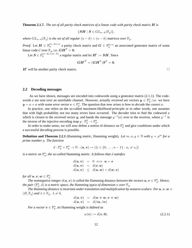
Theorem 2.1.7.The set of all parity check matrices of a linear code with parity check matrixH is
{SH | S ∈ GLn−k(Fq)},
whereGLn−k(Fq) is the set of all regular(n− k)× (n− k) matrices overFq.
Proof. Let H ∈ F(n−k)×nq a parity check matrix andG ∈ F
k×nq an associated generator matrix of some
linear codeC overFq, i.e.GHT = 0.
LetS ∈ F(n−k)×(n−k)q a regular matrix and letH ′ := SH. Since
GH ′T = (GHT )ST = 0,
H ′ will be another parity check matrix.
2.2 Decoding messages
As we have shown, messages are encoded into codewords using a generator matrix (2.1.1). The code-wordsc are sent over an unreliable channel. However, actually received arevectorsy ∈ F
nq , i.e. we have
y = c+ e with some error vectore ∈ Fnq . The question that now arises is how todecodethe correctc.
In practice, one relies on the so-calledmaximum-likelihood-principleor in other words, one assumesthat with high probability not too many errors have occurred. The decoder tries to find the codewordcwhich is closest to the received vectory, and hands the messageg−1(c) over to the receiver, whereg−1 isthe inverse of the injective encoding mapg : Fk
q → Fnq .
In order to make sense, we will now define a notion ofdistanceonFnq and give conditions under which
a successful decoding process is possible.
Definition and Theorem 2.2.1(Hamming metric, Hamming weight). Letm,n, q ∈ N with q = pm for aprime numberp. The function
d : Fnq × F
nq → N : (u,v) 7→ |{i ∈ {0, . . . , n− 1} : ui 6= vi}|
is a metric onFnq , the so-calledHamming metric. It follows thatd satisfies
d(u,v) = 0 ⇐⇒ u = v
d(u,v) = d(v,u)d(u,v) ≤ d(u,w) + d(w,v)
for all u,v,w ∈ Fnq .
The nonnegative integerd(u,v) is called theHamming distancebetween the vectorsu,v ∈ Fnq . Hence,
the pair(Fnq , d) is a metric space, theHamming spaceof dimensionn overFq.
The Hamming distance is invariant under translation and multiplication by nonzero scalars: Foru,v,w ∈(H,Fq) andλ ∈ Fq, λ 6= 0,
d(u,v) = d(u + w,v + w)d(u,v) = d(λu, λv)
For a vectorv ∈ Fnq , its Hamming weightis defined as
w(v) := d(v,0). (2.2.1)
12

Proof. The equivalenced(u,v) = 0 ⇐⇒ u = v and the symmetryd(u,v) = d(v,u) are trivial. Itremains to show the triangle equality.
Let u,v,w ∈ Fnq . Supposeui 6= vi for theith component. Thenui 6= wi or vi 6= wi, which establishes
the triangle equality. Using the linear structure ofFnq we haved(u,v) = d(u − v,0) = d(u +w −w −
v,0) = d(u+w,v+w). Similarly, forλ 6= 0, d(u,v) = d(u−v,0) = d(λ(u−v),0) = d(λu−λv,0) =d(λu, λv), which completes the proof.
Definition 2.2.2(Packing radius, minimum distance). Letn, t ∈ N, C a linear code overFq andx ∈ Fnq .
Bn(x, t) := {y ∈ Fnq | d(x,y) ≤ t} (2.2.2)
denotes the ball of radiust aroundx.
(i) Thepacking radiusof C is the largest integert, such that balls of radiust around codewords do notintersect:
pr(C) := maxc,c′∈C,c 6=c′
{t ∈ N | Bn(c, t) ∩ Bn(c′, t) = ∅} (2.2.3)
(ii) Theminimum distanceof C is defined as
d := dist(C) := min{d(c, c′) | c, c′ ∈ C, c 6= c′}. (2.2.4)
Remark 2.2.3. Using the linear structure ofFnq , i.e. d(u,v) = d(u− v,0) for u,v ∈ F
nq , we see that the
minimal distance of a linear codeC is equivalent with its minimal weight:
min{w(c) | c ∈ C, c 6= 0} = dist(C). (2.2.5)
Note that a[n, k]-codeC with minimal weightd is also denoted as[n, k, d]-code. Such a code is alsoknown as of type[n, k, d].
Theorem 2.2.4. The check matrixH of an [n, k, d]-code overFq with 0 < k < n has the followingproperties:
(i) H is an(n− k)× n matrix overFq of rankn− k.
(ii) Anyd− 1 columns are linearly independent.
(iii) There existd columns that are linearly dependent.
Conversely, any matrixH satisfying these properties is a check matrix of an[n, k, d]-code overFq.
Proof. (i): See (2.1).(ii): Assumes < d columns ofH linear dependent. In matrix form this means that there is ac ∈ F
nq
such thatcHT = 0 andw(c) = s < d. By definition ofH it follows thatc ∈ C. Contradiction.(iii) By assumption, there is a codewordc ∈ C, c 6= 0, w(c) = d. Becausec ∈ C, it follows that
cHT = 0, and therefore existd linear dependent columns.Conversely, letH ∈ F
(n−k)×nq with rankn − k. This means, that the setC′ := {x ∈ F
nq | xHT = 0}
is a subspace ofFnq with dimensionk. As before, we conclude thatd is the minimum distance ofC′.
As an immediate consequence of Theorem (2.2.4) we get:
Corollary 2.2.5. Every(n− k)× k matrix overFq, in which anyd− 1 columns are independent, is a checkmatrix of some[n, k]-codeC overFq with minimal distancedist(C) ≥ d.
13

≥ d ≥ 2t+ 1
c
c′
y
t
?
?
Figure 1: The maximum-likelihood-decoding method
Maximum likelihood-decoding Note that the minimal distanced of a linear codeC is a measurefor the quality of the code, i.e. for its error-correcting capabilities. Ifd ≥ 2t + 1, a decoder using themaximum-likelihood principle can correct up tot errors.
It is possible to correct up tot = ⌊(dist(C)− 1)/2⌋ (2.2.6)
errors in the following way [1]:
(i) Using maximum-likelihood-decoding, a vectory ∈ Fnq is decoded in a codewordc ∈ C, which is
closest toy with respect to the Hamming metric. In formal terms:y is decoded into a codewordc ∈ F
nq , such that
d(c,y) ≤ d(c′,y), ∀c′ ∈ C.
If there are severalc ∈ C with this property, one of them is chosen at random.
(ii) If the codewordc ∈ C was sent and no more thant errors occured during transmission, the receivedvector is
y = c+ e ∈ Fnq ,
wheree denotes theerror vector. It satisfies
d(c,y) = d(e,0) ≤ t
and hencec is theunique element ofC which lies in a ball of radiust aroundy. A maximumlikelihood decoder yields this elementc, and so we obtain the correct codeword.
Remark 2.2.6. The packing radiust of a linear codeC is ⌊(dist(C)− 1)/2⌋.
14

2.3 Equivalence of codes and information sets
Definition 2.3.1(Isometry, equivalence). Let(Fnq , d) the Hamming space with Hamming metricd (n ∈ N).
(i) A bijective linear mapι : Fnq → F
nq with d(u,v) = d(ι(u), ι(v)) ∀u,v ∈ F
nq is calledisometry.6
(ii) Let ι be an isometry. Two[n, k]-codesC, C′ overFq are calledequivalentif ι(C) = C′.
Remark 2.3.2. The Hamming weight of a vectorv ∈ Fnq is invariant under an isometryι.
Indeed, letv ∈ Fnq . Thenw(v) = d(v,0) = d(ι(v), ι(0)) = d(ι(v),0) = w(ι(v)).
Let ι : Fnq → F
nq be an isometry. Like any other linear map onFn
q , it is uniquely determined by theimages of the unit vectors. By remark (2.3.2), isometries do not change the Hamming weight. Hence, unitsvectors are mapped to multiples of unit vectors. Conversely, each linear mapwith this property is clearly anisometry.
Remark 2.3.3. Isometries onFnq are expressed by those invertibleFn×n
q matrices, which contain in eachrow and column precisely one element ofFq.
Let J ∈ Fn×nq an isometry in matrix form,G ∈ F
k×nq a generator matrix of a[n, k]-codeC overFq.
Hence,GJ is justG with some columns permutated and/or multiplied by some non-zero field element. Onthe other, hand we can also multiplyG from the left by some invertibleB ∈ F
kq without leaving the codeC.
It follows that we can apply toG theGaussian algorithm. Multiplication with someB will generate unitvectors in certain colums, which can be shifted afterwards by multiplication from the right with isometries.
Definition and Theorem 2.3.4(Systematic encoding, information sets). For each[n, k]-codeC with gener-ator matrixG there exists an equivalent[n, k]-codeC′ with generator matrixG′ of the form
G′ = (Ik|A), (2.3.1)
whereIk ∈ Fk×kq denotes thek × k identity matrix andA ∈ F
k×(n−k)q . The corresponding encoding
v 7→ vG′ (v ∈ Fkq ) is calledsystematic encodingandG′ a systematic generator matrixof C′.
The firstk coordinates of codewordsc ∈ C′ are called itsinformation set, the remainingn − k placesare known asredundancy set7.
Remark 2.3.5. When using systematic encodingv 7→ vG′ = v(Ik|A) = w, the firstk coordinatessimply repeat thek components of the messagev. However, errors may also have occured in the firstkcoordinates, so decoding by simply reading out the firstk coordinates values does not work. But if weare given the values of a codeword on these firstk coordinates, then the remainingn − k coordinates areuniquelydetermined. For letH ′ a corresponding check matrix, i.e.G′H ′T = 0. It follows by inspectionthatH ′ = (−AT |In−k). Two codewordsc, c′ which coincide in the firstk coordinates must therefore beequal in the lastn− k coordinates as well.
6Obvious isometries are the permutations of the coordinates.7They are also calledcheck bits, since they may be used for error correction and error detection.
15

2.4 Generalized Reed Solomon codes
Notation 2.4.1. 8 For 1 ≤ k ≤ n ∈ N denote the subspaces of all polynomials overFq of degree strict lessthank by
Fq[X]<k :=k−1⊕
i=0
FqXi.
Let n ≤ q ∈ N, L = (L0, . . . , Ln−1) an n-tuple of pairwise distinct elements ofFq andβ =(β0, . . . , βn−1) an n-tuple on nonzero elements ofFq.
Definition 2.4.2 (Generalized Reed-Solomon code). For 1 ≤ k ≤ n ∈ N we define theGeneralizedReed-Solomon-CodeGRSk(L,β) as
GRSk(L,β) := {(f(L0)β0, . . . , f(Ln−1)βn−1) | f(X) ∈ Fq[X]<k}. (2.4.1)
We add an equivalent, more explicit formulation of (2.4.1). Consider the following notations:
Φ(L) := (Lij)0≤i<k, 0≤j<n
:=
1 1 . . . 1L0 L1 . . . Ln−1
L20 L2
1 . . . L2n−1
......
......
Lk−10 Lk−1
1 . . . Lk−1n−1
∈ Fk×nq ,
∆(β) :=
β0 0 . . . 00 β1 . . . 0...
.... . .
...0 0 0 βn−1
∈ Fn×nq ,
f(X)Φ(L) := (f0, . . . , fk−1)Φ(L) = (f(L0), . . . , f(Ln−1)),
Γ :=
β0 β1 . . . βn−1
L0β0 L1β1 . . . Ln−1βn−1
L20β0 L2
1β1 . . . L2n−1βn−1
......
......
Lk−10 β0 Lk−1
1 β1 . . . Lk−1n−1βn−1
= Φ(L)∆(β) ∈ Fk×nq .
(2.4.2)
Using these notations we see thatGRSk(L,β) is formally generated in the following way:
GRSk(L,β) = {f(X)Γ | f(X) ∈ Fq[X]<k}. (2.4.3)
Remark 2.4.3. AsΦ(L) is a submatrix of the Vandermonde matrix and∆(β) is invertible,Φ(L) andΓ dohave rankk.
An important point to note here is that the sequenceβ can be replaced by a polynomialg(X) ∈ Fq[X],which later will be used to define so-called Goppa codes. To this end, we first recall some definitions andwell-known facts.
LetR andS commutative rings with 1.
8For the following explanations, see [1].
16

Definition 2.4.4(Ideal, principal ideal, relatively prime ideals).
(i) A subgroup (I,+) of (R,+) is calledideal iff ax ∈ I for all a ∈ R andx ∈ I.
(ii) For a ∈ R theprincipal ideal〈a〉 generated bya is defined as
〈a〉 := (a) := {ar | r ∈ R}.
(iii) Let I1, s, In ideals in R(n ≥ 2). They are calledrelatively prime(or coprime) iff Ik + Il = R fork 6= l.
Theorem 2.4.5.Letφ: R→ S a surjective ring homomorphism. The induced homomorphism
h : R/ kerφ→ S (a+ kerφ 7→ φ(a))
is a ring isomorphism.
Proof. [18], (6.11).
Theorem 2.4.6.Let I1, . . . , In relatively prime ideals in R(n ≥ 2). The canonical ring homomorphism
α : R −→ R/I1 × · · · × R/In
r 7→ (r + I1, . . . , r + In)
is an epimorphism with kernel
ker α =n⋂
i=1
Ii.
Proof. [18], (6.24).
Combining (2.4.6) and (2.4.5) yields:
Theorem 2.4.7(Chinese Remainder Theorem (CRT)).
R/n⋂
k=1
Ik ≃ R/I1 × · · · × R/In, (2.4.4)
(r +
n⋂
k=1
Ik 7→ (r + I1, . . . , r + In)).
In other words, theorem (2.4.7) states that for pairwise relatively prime ideals I1, . . . , In, n ≥ 2 andarbitrary elementsr1, . . . , rn ∈ R, there is always a solution for the system
X ≡ r1 mod I1...
X ≡ rn mod In,
(2.4.5)
and that for a particular solutionr the set of all solutions isr +⋂n
k=1 Ik.We finally note:
17

Lemma 2.4.8. A cosetr + I ∈ R/I is a unit ofR/I if and only ifI(r) = 〈r〉 andI are relatively prime.
Proof. [18], (6.32).
Consider now
h(X) :=n−1∏
i=0
(X − Li), (2.4.6)
and denote by〈h〉 the principal ideal inFq[X] generated byh(X):
〈h〉 = {hg | g ∈ Fq[X]} =n−1⋂
i=0
〈X − Li〉,
As theLi (0 ≤ i < n) are pairwise distinct, theX−Li are relatively prime inFq[X] and theorem (2.4.7)states:
Fq[X]/〈h〉 ∼= Fq[X]/〈X − L0〉 × . . . × Fq[X]/〈X − Ln−1〉.Polynomial division gives fori ∈ {0, . . . , n− 1} andf(X) ∈ Fq[X] a unique representation as:
f(X) = q(X)(X − Li) + f(Li),
whereq(X) ∈ Fq[X]. Thus we have anFq- algebra isomorphism
Φ: Fq[X]/〈h〉 ≃−→ Fnq
f + 〈h〉 7→ (f(L0), . . . , f(Ln−1))
This map restricts to an isomorphism between the two groups of units, which arethe polynomialsg(X) ∈ Fq[X]/〈h〉 with g(Li) 6= 0 for 0 ≤ i < n on one side (due to lemma (2.4.8)) and(F×
q )n, the se-
quences of lengthn overFq whose entries are all non-zero, on the other side (where we have the Hadamardproduct resp. componentwise multiplication):
Φ: (Fq[X]/〈h〉)× −→ (F×q )
n (2.4.7)
g + 〈h〉 7→ (g(L0), . . . , g(Ln−1)). (2.4.8)
In the other direction, given a sequencec = (c0, . . . , cn−1) with ci 6= 0 for 0 ≤ i < n, we obtain theinverse image under the mapΦ via Lagrange’s interpolation formula. Namely, we have
Φ−1 : (F×q )
n −→ Fq[X]/〈h〉 (2.4.9)
c = (c0, . . . , cn−1) 7→n−1∑
i=0
cil(Li)
n−1∏
j=0j 6=i
(X − Lj) + 〈h〉, (2.4.10)
wherel(X) is the unique polynomial of degree less thann with
l(Li) :=n−1∏
j=0j 6=i
(Li − Lj), (2.4.11)
18

and is given by Lagrange in explicit form as
l(X) =n−1∑
i=0
l(Li)
∏n−1j=0j 6=i
(X − Lj)
∏n−1j=0j 6=i
(Li − Lj)=
n−1∑
i=0
n−1∏
j=0j 6=i
(X − Lj). (2.4.12)
By construction, the residue classl + 〈h〉 is a unit inFq[X]/〈h〉. It serves in the following as a normal-izing factor. For each unitg + 〈h〉 we build the following linear code (which is isometric toGRSk(L, 1n),where1 := (1, 1, . . . , 1) ∈ F
nq ).
Definition 2.4.9.GRSk(L, g) := GRSk(L,β) (2.4.13)
whereβ = (β0, . . . , βn−1) is the sequence whose entries areβi =g(Li)
l(Li).
Theorem 2.4.10.
GRSk(L, g) =
{(c1g(L0)
l(L0), . . . ,
cn−1g(Ln−1)
l(Ln−1)
)
| c ∈ GRSk(L, 1n)
}
(2.4.14)
Proof. Let c ∈ GRSk(L, g) andβ =(g(L0)l(L0)
, . . . , g(Ln−1)l(Ln−1)
)
.
Using the notations (2.4.2), there existsf(X) ∈ Fq[X]<k such that
c = f(X)Γ= f(X)φ(L)∆(β)
= c′∆(β),
wheref(X)φ(L) =: c′ ∈ GRSk(L, 1n). This shows (2.4.14).
The following theorem will show extremely useful characterizations ofGRSk(L, g) codes. They willbe used below for the definition of alternant and Goppa codes.
Theorem 2.4.11.Let1 ≤ k ≤ n ≤ q ∈ N.LetL = (L0, . . . , Ln−1) be a sequence of pairwise distinct elements ofFq and
h(X) :=n−1∏
i=0
(X − Li).
Letg(X) ∈ Fq[X]<n with g(Li) 6= 0 for all 0 ≤ i < n.
GRSk(L, g) =
{
c ∈ Fnq
∣∣ ∃f(X) ∈ Fq[X]<k :
n−1∑
i=0
ci
n−1∏
j=0j 6=i
(X − Lj) ≡ fg mod 〈h〉}
(2.4.15)
If deg g(X) = n− k, then
GRSk(L, g) =
{
c ∈ Fnq
∣∣ ∃f(X) ∈ Fq[X]<k :
n−1∑
i=0
ci
n−1∏
j=0j 6=i
(X − Lj) ≡ 0 mod 〈g〉}
. (2.4.16)
19

GRSk(L, g) can also be characterized as the set of allc ∈ Fnq which satisfies
n−1∑
i=0
ci(X − Li)−1 = 0 (2.4.17)
in Fq[X]/〈g〉.
Proof. Let c ∈ Fnq .
As in the proof of (2.4.14) we see thatc ∈ GRSk(L, g) if and only if there exists a polynomialf(X) ∈Fq[X]<k such that
c =
(f(L0)g(L0)
l(L0), . . . ,
f(Ln−1)g(Ln−1)
l(Ln−1)
)
Recall that on(F×q )
n the multiplication is defined componentwise, see (2.4.7). Therefore, we get
(c0l(L0), . . . , cn−1l(Ln−1)) = (fg(L0), . . . , fg(Ln−1)) = φ(fg + 〈h〉)
(2.4.9)⇒ fg + 〈h〉 = φ−1(c0l(L0), . . . , cn−1l(Ln−1))
(2.4.10)⇒ fg =∑n−1
i=0 ci∏n−1
j=0j 6=i
(X − Lj) mod 〈h〉
Let deg g(X) = n − k andc ∈ GRSk(L, g) a codeword. According to the last shown equation, thereexist polynomialsf(X) ∈ Fq[X]<k ands(X) ∈ Fq[X] with
n−1∑
i=0
ci
n−1∏
j=0j 6=i
(X − Lj) = f(X)g(X) + s(X)h(X).
Becausedeg f(X) < k, it follows thatdeg f(X)g(X) < n = deg h(X), which implies
n−1∑
i=0
ci
n−1∏
j=0j 6=i
(X − Lj) = f(X)g(X),
and which is finally equivalent to
n−1∑
i=0
ci
n−1∏
j=0j 6=i
(X − Lj) ≡ 0 mod 〈g〉.
Using (2.4.8), it follows thath+ 〈g〉 is a unit inFq[X]/〈g〉. Multiplication by its inverse yields therefore inFq[X]/〈g〉
n−1∑
i=0
ci(X − Li)−1 = 0.
Since these arguments can be reversed, we obtain the assertion.
20

2.4.1 Alternant codes
The class of alternant codes is obtained by restrictingGRS-codes to subfields which means we now startwith an extension fieldFqm .
Definition 2.4.12(Subfield subcode). Consider the field extensionFqm/Fq. Let C ⊆ (Fqm)n be a code
overFqm .C|Fq := C ∩ F
nq (2.4.18)
is called thesubfield subcodeof C (or therestrictionof C to Fq).
Remark 2.4.13. Note that the dimension ofC is its dimension as a vector space overFqm , whereas thedimension ofC|Fq is the dimension as a vector space overFq.9
Proposition 2.4.14.Restricting codes defined over an extension fieldFqm reduces in general the code di-mension:
dim C|Fq ≤ dim C.
Proof. The inequality follows from the fact that a basis ofC|Fq overFq is also linearly independent overFqm [35]. Indeed, let(αi)i=1,...,n be aFq-basis ofC|Fq and
∑ni=1 aiαi = 0, whereai ∈ Fqm . To show is
thatai = 0 for all i = 1, . . . , n.Let (βi)j=1,...,m be aFq-basis ofFqm andai =
∑mj=1 bjβj , with bj ∈ Fq.
0 =n∑
i=1
aiαi =n∑
i=1
(m∑
j=1
bjβj)αi =m∑
j=1
(n∑
i=1
bjαi)βj .
Because(βi)j=1,...,m is a basis, it follows that∑n
i=1 bjαi = 0 for all j = 1, . . . ,m. As thebj are inFq and(αi)i=1,...,n is anFq-basis, this meansbj = 0 for all j = 1, . . . ,m. Hence,ai = 0 for all i = 1, . . . , n.
Definition 2.4.15(Alternant code). The restriction ofGRSk(L, g) overFqm to the subfieldFq is calledalternant code overFq, denoted as
Altk,q(L, g) := GRSk(L, g) ∩ Fnq . (2.4.19)
2.4.2 Goppa codes
Definition 2.4.16(Goppa code). The restriction of aGRSk(L, g) code overFqm with deg g(X) = n − kto Fq is called a q-ary Goppa code. It is a special alternant code and indicatedbyGOq(L, g):
GOq(L, g) := GRSk(L, g) ∩ Fnq , (2.4.20)
wheredeg g(X) = n− k.
Remark 2.4.17. According to Theorem(2.4.11), the Goppa codeGOq(L, g) has the form
GOq(L, g) =
{
c ∈ Fnq
∣∣
n−1∑
i=0
ci
n−1∏
j=0j 6=i
(X − Lj) ≡ 0 mod 〈g〉}
=
{
c ∈ Fnq
∣∣
n−1∑
i=0
ciX − Li
≡ 0 mod 〈g〉}
,
wheredeg g(X) = n− k.
9See [35].
21

Lemma 2.4.18.SupposeF an arbitrary field,L ∈ F, g(X) ∈ F[X], deg g(X) = t > 0 and g(L) 6= 0.Then there exists a uniquely determindedh(X) ∈ F[X], deg h(X) < t, such that
(X − L)h(X) ≡ 1 mod g(X). (2.4.21)
Proof. Indeed, using division by remainder, it follows thatg(L) − g(X) = α(X)(X − L) + r(X), whereα(X), r(X) ∈ F[X]. InsertingL on both sides givesr(X) = 0. Hence,X − L dividesg(L) − g(X) andwe can defineh(X) ∈ F[X] as
h(X) :=g(L)− g(X)
g(L)(X − L).
Sincedeg g(X) = t, it is immediate thatdeg h(X) < t. We apply division with remainder again to thepolynomial(X − L)h(X)− 1. For degree reasonsα(X) has to be a constant:
(X − L)h(X)− 1 = α(X)g(X) + r(X) = αg(X) + r(X).
Using the definition ofh(X) gives−r(X)g(L) = (αg(L) + 1)g(X). Becausedeg g(X) = t, butdeg r(X) < t, we concludeαg(L) + 1 = 0 and finally becauseg(L) 6= 0, that r(X) = 0. Thisproves (2.4.21).
For the uniqueness, assume thath(X), h′(X) solve (2.4.21). Thusg(X) divides(X −L)h(X)− 1 and(X−L)h′(X)− 1 and consequently also their difference(X−L)(h(X)−h′(X)). But g(X) and (X−L)are relatively prime, which means thatg(X) divides(h(X) − h′(X)). Becausedeg(h(X) − h′(X)) < tanddeg g(X) = t, it follows thath(X) = h′(X).
Remark 2.4.19. Under the assumptions of Lemma(2.4.18)we write
1
X − L=
g(L)− g(X)
g(L)(X − L), (2.4.22)
but this notation is a bit sloppy.1/(X − L) is not a polynomial. Rather, we identify a polynomialh(X) ∈F[X] and its residue class inF[X]/〈g〉. In this sense,1/(X − L) can be considered as polynomial, as longas we work modulo a polynomialg(X), which does not haveL as root.
2.4.2.1 Parity check matrix of a Goppa code. The check matrix of a code that restricts to a Goppa codeGOq(L, g) can be obtained in the following way:10
According to remark (2.4.17) and lemma (2.4.18) anc ∈ Fnq is contained inGOq(L, g) if and only if
n−1∑
i=0
cig(X)− g(Li)
X − Lig(Li)
−1 = 0 (2.4.23)
in Fqm [X]/〈g〉. As
deg(g(X)− g(Li))
(X − Li)< deg g(X),
equation (2.4.23) can be considered as an equation inFqm [X]:
n−1∑
i=0
cig(X)− g(Li)
X − Lig(Li)
−1 = 0. (2.4.24)
10[26], pp. 390 – 393, with minor corrections by the author.
22
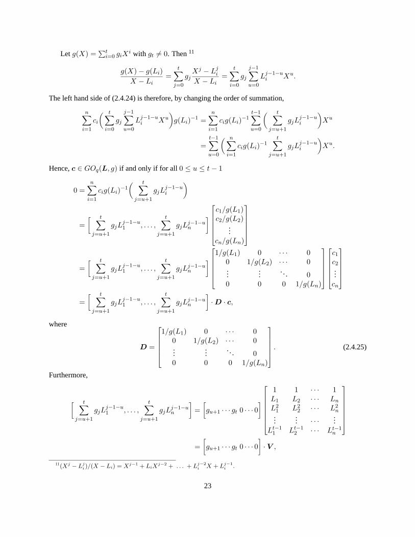
Let g(X) =∑t
i=0 giXi with gt 6= 0. Then11
g(X)− g(Li)
X − Li=
t∑
j=0
gjXj − Lj
i
X − Li=
t∑
i=0
gj
j−1∑
u=0
Lj−1−ui Xu.
The left hand side of (2.4.24) is therefore, by changing the order of summation,
n∑
i=1
ci
( t∑
i=0
gj
j−1∑
u=0
Lj−1−ui Xu
)
g(Li)−1 =
n∑
i=1
cig(Li)−1
t−1∑
u=0
( t∑
j=u+1
gjLj−1−ui
)
Xu
=t−1∑
u=0
( n∑
i=1
cig(Li)−1
t∑
j=u+1
gjLj−1−ui
)
Xu.
Hence,c ∈ GOq(L, g) if and only if for all 0 ≤ u ≤ t− 1
0 =n∑
i=1
cig(Li)−1
( t∑
j=u+1
gjLj−1−ui
)
=
[ t∑
j=u+1
gjLj−1−u1 , . . . ,
t∑
j=u+1
gjLj−1−un
]
c1/g(L1)c2/g(L2)
...cn/g(Ln)
=
[ t∑
j=u+1
gjLj−1−u1 , . . . ,
t∑
j=u+1
gjLj−1−un
]
1/g(L1) 0 · · · 00 1/g(L2) · · · 0...
..... . 0
0 0 0 1/g(Ln)
c1c2...cn
=
[ t∑
j=u+1
gjLj−1−u1 , . . . ,
t∑
j=u+1
gjLj−1−un
]
·D · c,
where
D =
1/g(L1) 0 · · · 00 1/g(L2) · · · 0...
.... . . 0
0 0 0 1/g(Ln)
. (2.4.25)
Furthermore,
[ t∑
j=u+1
gjLj−1−u1 , . . . ,
t∑
j=u+1
gjLj−1−un
]
=
[
gu+1 · · · gt 0 · · · 0]
1 1 · · · 1L1 L2 · · · Ln
L21 L2
2 · · · L2n
...... · · · ...
Lt−11 Lt−1
2 · · · Lt−1n
=
[
gu+1 · · · gt 0 · · · 0]
· V ,
11(Xj − Lji )/(X − Li) = Xj−1 + LiX
j−2 + . . . + Lj−2i X + Lj−1
i .
23

whereV resembles in structure the Vandermonde matrix,12
V =
1 1 · · · 1L1 L2 · · · Ln
L21 L2
2 · · · L2n
...... · · · ...
Lt−11 Lt−1
2 · · · Lt−1n
.
Summarizing, this means that (2.4.24) holds if and only if for all0 ≤ u ≤ t− 1
[
gu+1 · · · gt 0 · · · 0]
· V ·D · c = 0,
that is, if and only if
gt 0 0 · · · 0gt−1 gt 0 · · · 0gt−2 gt−1 gt · · · 0
......
... · · · ...g1 g2 g3 · · · gt
· V ·D · c = 0.
The canonical parity check matrixH for a GRS code, which restricts to a Goppa code, has therefore thefollowing form:
H =
gt 0 0 · · · 0gt−1 gt 0 · · · 0gt−2 gt−1 gt · · · 0
......
... · · · ...g1 g2 g3 · · · gt
1 1 . . . 1L0 L1 . . . Ln−1
L20 L2
1 . . . L2n−1
......
......
Lt−10 Lt−1
1 . . . Lt−1n−1
g(L0)−1 0 . . . 0
0 g(L1)−1 . . . 0
0 0 . . . 0...
.... . . 0
0 0 0 g(Ln−1)−1
.
(2.4.26)As the Toeplitz matrix on the left is invertible (gt 6= 0), this is equivalent to
V Dc = 0.
Hence, a parity check matrixH takes also the following form:
H = V D =
1 1 . . . 1L0 L1 . . . Ln−1
L20 L2
1 . . . L2n−1
......
......
Lt−10 Lt−1
1 . . . Lt−1n−1
g(L0)−1 0 . . . 0
0 g(L1)−1 . . . 0
......
. .. 00 0 0 g(Ln−1)
−1
(2.4.27)
With proposition (2.4.14) in mind, the following theorem is not surprising:
Theorem 2.4.20.The Goppa codeGO2(L, g), wheredeg g(X) = t < n, has lengthn = |L|, dimensionksatisfying
n−mt ≤ k ≤ n− t (2.4.28)
and minimum distanced ≥ t+ 1.12The Vandermonde matrix is quadratic, and transposed toV . Note also the similarity with (2.4.2).
24

Proof. See [26], Thm. (8.3.2), p. 393.
We consider now a special class of Goppa codes, so-calledbinary Goppa codes, i.e. Goppa codes withq = 2. As it will turn out, they have a fundamental property, which is of crucial importance for the securityof cryptosystems based on quasi-dyadic Goppa codes.
2.4.3 Binary Goppa codes
Definition 2.4.21(Binary Goppa code). The restriction of aGRSk(L, g) code overF2m with deg g(X) =n− k = t to F2 is called a binary Goppa code. It is a special alternant code and indicatedbyGO2(L, g):
GO2(L, g) := GRSk(L, g) ∩ Fn2 .
Because of its importance, let’s write down the above definition (2.4.21) explicitly. The ingredients of abinary Goppa code are the following:
(i) A monic polynomialg(X) of degreet = n− k,
g(X) =t∑
i=0
giXi ∈ F2m [X]. (2.4.29)
(ii) A tupleL of n pairwise distinct elements
L = (L0, . . . , Ln−1) ∈ Fn2m , (2.4.30)
such thatg(Li) 6= 0, i ∈ {0, . . . , n− 1}. (2.4.31)
Then the binary Goppa codeGO2(L, g) is
GO2(L, g) =
{
c = (c0, . . . , cn−1) ∈ Fn2
∣∣
n−1∑
i=0
ciX − Li
≡ 0 mod g(X)
}
. (2.4.32)
Remark 2.4.22.The elementsL0, . . . , Ln−1 ∈ F2m are also calledcode support, whereasg(X) ∈ F2m [X]is referred to asGoppa polynomial.
Sc(X) := −n−1∑
i=0
cig(Li)
g(X)− g(Li)
X − Limod g(X) (2.4.33)
is known as thesyndrome polynomialof c. The binary Goppa codeGO2(L, g) consists of allc =(c0, . . . , cn−1) ∈ F
n2 such that
Sc(X) ≡n−1∑
i=0
ciX − Li
≡ 0 mod g(X). (2.4.34)
25

Consider now a codewordc = (c0, . . . , cn−1) ∈ GO2(L, g) with some Hamming weightw(c) = ω,i.e. ci1 = · · · = ciω = 1, whereas the other coordinates are0 (see [26], with some additions by the author).If
fc(X) :=ω∏
j=1
(X − Lij ), (2.4.35)
then the formal derivative offc(X) is
fc(X)′ =ω∑
k=1
∏
j 6=k
(X − Lij ), (2.4.36)
and furtherSc(X)fc(X) = f ′
c(X). (2.4.37)
Note thatfc(X) andg(X) are relatively prime: because ofg(Li) 6= 0, they have no common roots inany extension. Hence,
c ∈ GO2(L, g) ⇐⇒ g(X)|Sc(X) ⇐⇒ g(X)|fc(X)′. (2.4.38)
Remark 2.4.23.Because we are in characteristic 2,fc(X)′ =∑n
i=1 ifiXi−1 contains only even powers of
X. Furthermore, it is a perfect square, i.e.fc(X)′ = h(X2) = k(X)2 for some polynomialsh(X), k(X) ∈F2m [X].
Proof. The mapF2m → F2m , a 7→ a2 is the Frobenius automorphism onF2m . Therefore, each elementa ∈ F2m has a unique square root. Givenh(X) =
∑akX
2k ∈ F2m [X], definek(X) =∑√
akXk. Then
k(X)2 = h(X).
Lemma 2.4.24.Let g(X) the perfect square with smallest degree, which is divisible byg(X), i.e. g(X) =α(X)g(X) for someα(X) ∈ F2m [X]. Then
g(X)|fc(X)′ ⇐⇒ g(X)|fc(X)′. (2.4.39)
Proof. ⇒: fc(X)′ = γ(X)g(X) = γ(X)α(X)g(X) for someγ(X) ∈ F2m [X]. ⇐: Let g(X) =α(X)g(X), g(X) a perfect square. Becauseg(X)|fc(X)′, it follows thatdeg g(X) ≤ deg fc(X)′ (be-causefc(X)′ is a perfect square according to (2.4.23) and the minimality ofg(X)). Thereforefc(X)′ =β(X)g(X) + r(X) = β(X)α(X)g(X) + r(X). By assumption, we haver(X) = 0, which finally givesg(X)|fc(X)′.
The next theorem will summarize the latest results:
Theorem 2.4.25.LetGO2(L, g) be a binary Goppa code. Ifg(X) is the polynomial of smallest degree thatis a perfect square and is divisible byg(X), then
GO2(L, g) = GO2(L, g). (2.4.40)
In particular,GO2(L, g) has a minimum distance at leastdeg g(X) + 1.
26

Proof. Let c ∈ GO2(L, g).
c ∈ GO2(L, g)Def.⇐⇒ Sc(X) ≡ 0 mod g(X)
(2.4.38)⇐⇒ g(X)|fc(X)′
(2.4.39)⇐⇒ g(X)|fc(X)′
(2.4.38)⇐⇒ Sc(X) ≡ 0 mod g(X)Def.⇐⇒ c ∈ GO2(L, g)
For the statement about the minimum distance, see (2.4.20).
Corollary 2.4.26. 13 LetGO2(L, g) be a binary Goppa code and suppose that the Goppa polynomialg(X)has no multiple roots in any extension field. Then
GO2(L, g) = GO2(L, g2). (2.4.41)
In particular, the minimum distance ofGO2(L, g) is at least2 deg g(X)+1. Hence,GO2(L, g) can correctat leastdeg g(X) errors.
Definition 2.4.27(Irreducible Goppa code, separable Goppa code).
(i) A binary Goppa code with a Goppa polynomial irreducible overFq is called a irreducibleGoppacode.
(ii) A binary Goppa code whose Goppa polynomial has no multiple roots in any extension field is calleda separableGoppa code.
Remark 2.4.28.The crucial meaning of Cor.(2.4.26)is the fact that separable binary Goppa codes have twodifferent representations withdifferenterror correcting capabilities. In other words, an alternant decoderbased ong(X)2 can correct twice as much errors as a decoder based ong(X).
2.4.4 Examples for binary Goppa codes
2.4.4.1 Example Let 14 g(X) = x2 + x + 1 and the supportL = {0, 1, ω, . . . , ω6} = F8. Thusm = 3, t = 2, n = 8 andω is a primitive element ofF8. The zeros ofg(X) are not inF8, but in F4. If wewrite F4 as F4 = {0, 1, z, z2}, then the zeros arez andz2, as is easily calculated.
The parity check matrixH ′ of the Goppa codeGO2(L, g) is obtained from the matrix
H =
[
1/g(0) 1/g(1) 1/g(ω) . . . 1/g(ω6)0/g(0) 1/g(1) ω/g(ω) . . . ω6/g(ω6)
]
=
[
1 1 ω2 ω4 ω2 ω ω ω4
0 1 ω3 ω6 ω5 ω5 ω6 ω3
]
,
13Nicola Sendrier calls it the binary miracle. It will be the key of the quasi-dyadic cryptosystem, as will be shown below.14[26], p. 394.
27

which can be seen by using a field table ofF8. As the Goppa code is a subfield subcode, we need to expressthe entries ofH as vectorsa = (a0, a1, a2) with ai ∈ F2 ([20], Ch. 7, p. 207).
H ′ =
1 1 0 0 0 0 0 00 0 0 1 0 1 1 10 0 1 1 1 0 0 10 1 1 1 1 1 1 10 0 1 0 1 1 0 10 0 0 1 1 1 1 0
.
Since the rank ofH ′ is 6, dimGO2(L, g) = 2 and with some calculation it follows that
GO2(L, g) = {00000000, 11110100, 11001011, 00111111},
hence the Goppa code has a minimum distance of5.
2.4.4.2 Example Let 15 g(X) = x2 + 1 and the supportL = {0, ω, ω2, ω3, ω5, ω6} ⊂ F8. Thusm =3, t = 2, n = 6 andω is again a primitive element ofF8. As charF8 = 2, it holds thatg(X) = (X + 1)2.Using corollary (2.4.26) we see thatGO2(L, g) = GO2(L, X + 1). By theorem (2.4.20), we conclude thedimensionk to be greater thann−mt = 6− 3 · 1 = 3. Furthermore,
H =
[1
0 + 1
1
ω + 1
1
ω2 + 1
1
ω3 + 1
1
ω4 + 1
1
ω5 + 1
]
=[
1 ω4 ω ω6 ω3 ω5]
,
and thus a parity check matrix forGO2(L, g) is
H ′ =
1 1 0 1 0 10 1 1 0 1 10 0 0 1 1 1
,
and we see thatGO2(L, g) has minimum distance3.
2.4.5 Parity check matrix generated byg(X)2 in case of a binary, separable Goppa codes
Let Z = {z0, . . . , zt−1} ⊂ F2m andL = {L0, . . . , Ln−1} ⊂ F2m , where all the members ofL are distinct.LetZ ∩L = ∅ and define the Goppa polynomialg(X) without multiple roots as
g(X) = (X − z0) · · · (X − zt−1) ∈ F2m [X],
wheret < n.Using (2.4.27), we see that a parity check matrixH ′ for the Goppa codeGO2(L, g2) is given as:
15[26], p. 395.
28

H ′ = V D =
1 1 · · · 1L0 L1 · · · Ln−1
L20 L2
1 · · · L2n−1
......
......
Lt−10 Lt−1
1 · · · Lt−1n−1
Lt0 Lt
1 · · · Ltn−1
......
......
L2t−10 L2t−1
1 · · · L2t−1n−1
g(L0)−2 0 · · · 0
0 g(L1)−2 · · · 0
......
. .. 00 0 0 g(Ln−1)
−2
. (2.4.42)
As in (2.4.26), it is also possible to add the corresponding Toeplitz matrix on theleft, of course16.
2.4.6 Parity check matrix generated byg(X)2 in Tzeng-Zimmermann form
To derive another form (see [36]) for the parity check matrixH ′ for the Goppa codeGO2(L, g2) generatedby
g(X)2 = (X − z0)2 · · · (X − zt−1)
2,
apply (2.4.27) togl(X) = (X − zl)2, where0 ≤ l ≤ t − 1. Because it is allowed to add a row of a parity
check matrix, multiplied by a common factor, to any other row of the matrix, we havefor gl(X) as a paritycheck matrixH l:
H l =
[
(L0 − zl)−2 (L1 − zl)
−2 · · · (Ln−1 − zl)−2
L0(L0 − zl)−2 L1(L1 − zl)
−2 · · · Ln−1(Ln−1 − zl)−2
]
;
[
(L0 − zl)−2 (L1 − zl)
−2 · · · (Ln−1 − zl)−2
(L0 − zl)(L0 − zl)−2 (L1 − zl)(L1 − zl)
−2 · · · (Ln−1 − zl)(Ln−1 − zl)−2
]
;
[
(L0 − zl)−2 (L1 − zl)
−2 · · · (Ln−1 − zl)−2
(L0 − zl)−1 (L1 − zl)
−1 · · · (Ln−1 − zl)−1
]
;
[
(L0 − zl)−1 (L1 − zl)
−1 · · · (Ln−1 − zl)−1
(L0 − zl)−2 (L1 − zl)
−2 · · · (Ln−1 − zl)−2
]
It is easily seen that the Goppa codeGO2(L, g2) is the intersection of the Goppa codesGO2(L, gl),
GO2(L, g2) =t−1⋂
l=0
GO2(L, gl).
Hence, we have
16These two matricesH andH ′ are leading to slightly different key equations, however. For the decoder, we will use theToeplitz-formH.
29

H ′ =
H0
H1...
Ht−1
=
(L0 − z0)−1 (L1 − z0)
−1 · · · (Ln−1 − z0)−1
(L0 − z0)−2 (L1 − z0)
−2 · · · (Ln−1 − z0)−2
(L0 − z1)−1 (L1 − z1)
−1 · · · (Ln−1 − z1)−1
(L0 − z1)−2 (L1 − z1)
−2 · · · (Ln−1 − z1)−2
......
...(L0 − zt−1)
−1 (L1 − zt−1)−1 · · · (Ln−1 − zt−1)
−1
(L0 − zt−1)−2 (L1 − zt−1)
−2 · · · (Ln−1 − zt−1)−2
. (2.4.43)
More general, we have:
Theorem 2.4.29.The Goppa code generated by a monic polynomialg(X) without multiple zerosg(X) =(X − z0) . . . (X − zt−1) admits a parity-check matrix of the formH = C(z, L), i.e. Hij = 1/zi − Lj ,0 ≤ i < t, 0 ≤ j < n.
Proof. See [20], Ch. 12, p. 345, Problem 5. or [36], p. 713.
Remark 2.4.30. Goppa codes in Tzeng-Zimmermann form turn out to be special cases ofso-calledSrivas-tava codes. See [20] (Chap. 12, §6) or [25].
2.4.7 Goppa codes in Cauchy and dyadic form
Definition 2.4.31(Dyadic matrix, quasi-dyadic matrix, signature [3]). Let r = 2k for somek ∈ N.
(i) Given a ringR and a vectorh = (h0, . . . , hr−1) ∈ R, the dyadic matrix∆(h) ∈ Rr×r is thesymmetric matrix with components∆ij = hi⊕j , where⊕ stands for the bitwise exclusive-or. Such amatrix is said to have orderk. The sequenceh is called itssignature. The set of dyadicr× r matricesoverR is denoted∆(Rr×r).
(ii) A quasi-dyadicmatrix is a (possibly non-dyadic) matrix, whose elements are dyadic submatrices, i.e.an element ofH(Rr).
Remark 2.4.32. It is easy to check that the signature of a dyadic matrix is nothing more than itsfirst row(column). By the definition of dyadic matrices, the signature is enough to rebuild the whole matrix. Hence,such a matrix allows a very compact represenation.
We give a visualization of such a matrix forr = 3:
H(h) := (hi⊕j) :=
A B C D E F G HB A D C F E H GC D A B G H E FD C B A H G F EE F G H A B C DF E H G B A D CG H E F C D A BH G F E D C B A
30

In the sequel, we will give the definition of a so-calledCauchy matrixand a theorem about Goppa codeshaving a Cauchy matrix as generating matrix. Afterwards, we will see how to connect Cauchy matrices anddyadic matrices.
Definition 2.4.33 (Cauchy matrix). Let z = (z0, . . . , zt−1) ∈ Ftq and L = (L0, . . . , Ln−1) ∈ F
nq two
disjoint sequences of distinct elements.
TheCauchy matrixC(z, L) is the matrix with elementsCij =1
zi − Lj∈ Fq:
C(z, L) = (Cij) =
1z0−L0
1z0−L1
. . . 1z0−Ln−1
1z1−L0
1z1−L1
. . . 1z1−Ln−1
......
......
1zt−1−L0
1zt−1−L1
. . . 1zt−1−Ln−1
∈ Ft×nq (2.4.44)
The question now is if there are Cauchy matrices in dyadic form. The answeris yes, thereby having theadditional property of a very compact representation.
Theorem 2.4.34(Cauchy matrices in dyadic form [23]). LetH ∈ Fn×nq with n > 1 be simultaneously a
dyadic matrixH = ∆(h) for someh ∈ Fnq and a Cauchy matrixH = C(z, L) for two disjoint sequences
z ∈ Fnq andL ∈ F
nq of distinct elements. ThenFq is a binary field,h satisfies
1
hi⊕j=
1
hi+
1
hj+
1
h0, (2.4.45)
andzi = 1/hi + ω, Lj = 1/hj + 1/h0 + ω for someω ∈ Fq.
Remark 2.4.35. Dyadic matrices allow a very compact representation. Parity check matrices in Cauchyform can be generated by Goppa polynomials of the form
g(X) = (X − z0)(X − z1) · · · (X − zt−1).
Due to theorem(2.4.34), the intersection between dyadic matrices and Cauchy matrices is not empty: wehave to use valueszi andLj satisfying equation(2.4.45).
As noted in [23], a cryptosystem based on a parity-check matrix in Cauchy form would immediatelyreveal the Goppa polynomial as there would be an overdefined linear systemzi − Lj = 1/Hij consistingof tn equations int + n unknowns. Hence, additional techniques will have to be applied, in particular theuse of quasi-dyadic subfield subcodes as the most important. We will address some of these points in theimplementation section.
2.4.8 The fast Walsh-Hadamard transform and the dyadic convolution
By saving only the necessary signatures, dyadic and quasi-dyadic matrices allow a substantial reduction ofthe public key size. Instead of keeping a whole generator matrixG ∈ F
k×nq , for a purely dyadic code we
would only need its first row. The encryption of a messageu ∈ Fkq into the codewordc ∈ F
nq is done by the
vector-matrix productc = uG.
31

This raises the question of how to performuG efficiently in terms of time and space. If it would benecessary to expand the signatureh into the matrixG, then the scheme would be less useful. As it turnsout,uG can be done without expanding the signatureh using the Walsh-Hadamard transform [3, 15]
The following is taken from [3]. We make the same assumptions as for (2.4.31), in particular we alwaysassumer = 2k.
Definition 2.4.36 (Dyadic convolution). The dyadic convolution of two vectorsu,v ∈ R is the uniquevector denoted byu △ v ∈ R such that∆(u △ v) = ∆(u)∆(v). The dyadic inverse of a vectoru ∈ R,which exists wheneverdet∆(u) 6= 0, is the vectoru△1 such that∆(u△1) = ∆(u)−1.
Definition 2.4.37(Sylvester-Hadamard matrix). Let F be a field with characteristicchar(F) 6= 2. TheSylvester-Hadamard matrixHk ∈ F
r is recursively defined as
H0 =[
1]
Hk =
[
Hk−1 Hk−1
Hk−1 −Hk−1
]
, k > 0.(2.4.46)
Remark 2.4.38. It is easily seen that
H−10 =
[
1]
H−1k =
1
2
[
H−1k−1 H−1
k−1
H−1k−1 −H−1
k−1
]
, k > 0.(2.4.47)
Lemma 2.4.39.Let F be a field with characteristicchar(F) 6= 2. If M ∈ Fr×r is dyadic, thenH−1
k MHk
is diagonal.
Proof. We describe the proof as given in [3] for ease of reference. The assertion is obviously true fork = 0.Let k > 0, and write
M =
[
AB
BA
]
,
whereA andB are dyadic. It follows that
H−1k MHk =
1
2
[
H−1k−1 H−1
k−1
H−1k−1 −H−1
k−1
] [
AB
BA
] [
Hk−1 Hk−1
Hk−1 −Hk−1
]
=
[
Hk−1M+Hk 0
0 H−1k−1M−Hk−1
]
,
(2.4.48)
and because bothM+ = A +B andM− = A −B are dyadic,H−1k−1M+Hk−1 andH−1
k−1M−Hk−1
are diagonal by induction, so isH−1k MHk.
Remark 2.4.40.Lemma(2.4.39)suggests an efficient way to multiply two dyadic matricesM andN usingthe diagonal formsH−1
k MHk andH−1k NHk as
(H−1k MHk)(H
−1k NHk) = H−1
k (MN)Hk.
However, it is not necessary to carry outH−1k MHk completely in order to diagonalizeM , as the following
lemma(2.4.41)shows.
32

Lemma 2.4.41.Let F be a field with characteristicchar(F) 6= 2. The diagonal form of a dyadic matrixM ∈ F
r×r is the first line ofMHk. In other words,H−1k ∆(h)Hk = diag(hHk).
Proof. The statement is true fork = 0. Therefore, letk > 0, M =[ABBA
], M+ = A + B andM− =
A − B as before. By (2.4.48) the diagonal ofH−1k (M)Hk is the concatenation of the diagonals of
H−1k−1M+Hk−1 andH−1
k−1M−Hk−1. Similarly, since
MHk =
[
A B
B A
] [
Hk−1 Hk−1
Hk−1 −Hk−1
]
=
[
M+Hk−1 M−Hk−1
M+Hk−1 −M−Hk−1
]
,
the first line ofMHk is the concatenation of the first lines ofM+Hk−1 andM−Hk−1, which by inductionare the diagonals ofH−1
k−1M+Hk−1 andH−1k−1M−Hk−1, respectively.
Corollary 2.4.42. Computingw such that∆(u)∆(v) = ∆w involves only three multiplications of vectorsby Sylvester-Hadamard matrices.
Proof. By Lemma (2.4.41),
diag(uHk)diag(vHk) = (H−1k ∆(u)Hk)(H
−1k ∆(v)Hk)
= H−1k (∆(u)∆(v))Hk
= H−1k ∆(w)Hk
= diag(wHk).
Now retrievew from the vectorz = wHk asw = zH−1k = 2−kzHk.
Remark 2.4.43. The structure of Sylvester-Hadamard matrices leads to an efficient algorithm to computeuHk for u ∈ F
r, which is known as the fast Walsh-Hadamard transform.Let [u0,u1] be the two halves ofu. Then
uHk = [u0,u1]
[
Hk−1 Hk−1
Hk−1 −Hk−1
]
= [(u0 + u1)Hk−1, (u0 − u1)Hk−1], (2.4.49)
which is a recursive algorithm of complexityΘ(r log r).
The reader may have noticed that the general assumption for the conclusions above was always a fieldnot having characteristic 2. At first glance, this fact seems to exclude theWalsh-Hadamard transform as anefficient tool in the context of binary Goppa codes, but there is a solutionfor the problem. It consists oflifting the algorithm to characteristic0, namely fromF2 = Z/2Z to Z. What actually happens is that allthe bits involved in the calculations are seens as integers. By the end of the computation, the result will bereduced modulo2, see section (8.1) for details.
Another approach may be to compute the productuHk directly using only the signature ofHk forproper parameter settings. That means that during the multiplication process,the current row ofHk iscomputed on the fly. It might be good choice due to its small memory footprint, seesection (8.1) as well.
33
Part V
Code-based cryptosystems
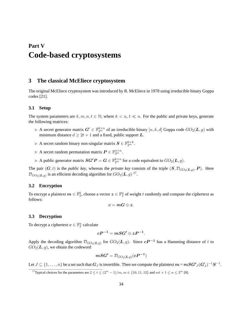
3 The classical McEliece cryptosystem
The original McEliece cryptosystem was introduced by R. McEliece in 1978using irreducible binary Goppacodes [21].
3.1 Setup
The system parameters arek,m, n, t ∈ N, wherek < n, t ≪ n. For the public and private keys, generatethe following matrices:
⊲ A secret generator matrixG′ ∈ Fk×n2m of an irreducible binary[n, k, d] Goppa codeGO2(L, g) with
minimum distanced ≥ 2t+ 1 and a fixed, public supportL.
⊲ A secret random binary non-singular matrixS ∈ Fk×k2m .
⊲ A secret random permutation matrixP ∈ Fn×n2m .
⊲ A public generator matrixSG′P = G ∈ Fk×n2m for a code equivalent toGO2(L, g).
The pair(G, t) is thepublic key, whereas theprivate keyconsists of the triple(S,DGO2(L,g),P ). HereDGO2(L,g) is an efficient decoding algorithm forGO2(L, g) 17.
3.2 Encryption
To encrypt a plaintextm ∈ Fk2, choose a vectorz ∈ F
n2 of weightt randomly and compute the ciphertext as
follows:c = mG⊕ z.
3.3 Decryption
To decrypt a ciphertextc ∈ Fn2 calculate
cP−1 = mSG′ ⊕ zP−1.
Apply the decoding algorithmDGO2(L,g) for GO2(L, g). SincecP−1 has a Hamming distance oft toGO2(L, g), we obtain the codeword
mSG′ = DGO2(L,g)(cP−1)
LetJ ⊆ {1, . . . , n} be a set such thatGJ is invertible. Then we compute the plaintextm =mSG′
J(G′J)
−1S−1.
17Typical choices for the parameters are2 ≤ t ≤ (2m − 1)/m, m ∈ {10, 11, 12} andmt+ 1 ≤ n ≤ 2m [8].
34

4 A modern McEliece cryptosystem
The private key for the McEliece scheme as described above consists ofthe Goppa polynomialg(X), SandP . The supportL is fixed and public. From an implementation point of view, it is more suitable towork with a permuted, secret support and to transform the matrixG′ to systematic form. As mentionedin [11], Section (3.1),S has no cryptographic function in hiding the secret polynomialg(X). The net effectis therefore that we can get rid of the matricesS andP [2].
4.1 Setup
The system parameters are as in section (3), except the supportL is secret and permuted.For the public and private keys, generate the following matrices:
⊲ A secret generator matrixG′ ∈ Fk×n2m of an irreducible binary[n, k, d] Goppa codeGO2(L, g) with
minimum distanced ≥ 2t+ 1 and a secret, permuted supportL.
⊲ A public generator matrixG ∈ Fk×n2m for a code equivalent toGO2(L, g) in systematic form.
Set theprivate keyKpriv = (L, g) and thepublic keyKpub = (G, t).
4.2 Encryption
To encrypt a plaintextm ∈ Fk2, we proceed as in the classical case, choosing a vectorz ∈ F
n2 of weight t
randomly and computing the ciphertext:c = mG⊕ z.
4.3 Decryption
The decryption of a ciphertextc ∈ Fn2 is considerable simpler than in the classical case: we just apply the
decoding algorithmDGO2(L,g) for GO2(L, g). Sincec has a Hamming distance oft to GO2(L, g), weobtain the codeword
mG′ = DGO2(L,g)(c)
No permutation is necessary, since it is hidden in the secret supportL, which is only used for the keygeneration process. SinceG is in systematic form, no multiplication with an invers matrixS−1 is necessaryas well. All what remains to be done is to read the infobits ofmG.
35
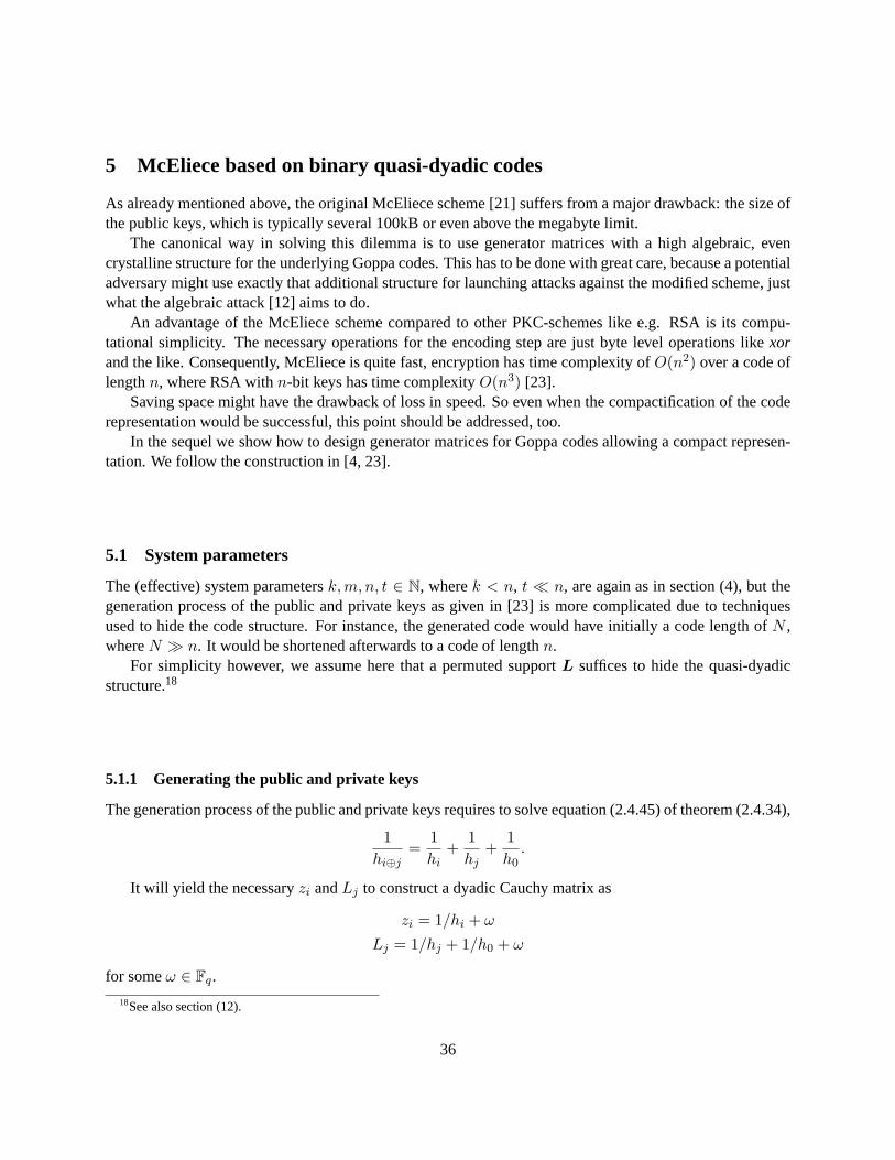
5 McEliece based on binary quasi-dyadic codes
As already mentioned above, the original McEliece scheme [21] suffers from a major drawback: the size ofthe public keys, which is typically several 100kB or even above the megabyte limit.
The canonical way in solving this dilemma is to use generator matrices with a high algebraic, evencrystalline structure for the underlying Goppa codes. This has to be donewith great care, because a potentialadversary might use exactly that additional structure for launching attacks against the modified scheme, justwhat the algebraic attack [12] aims to do.
An advantage of the McEliece scheme compared to other PKC-schemes like e.g. RSA is its compu-tational simplicity. The necessary operations for the encoding step are justbyte level operations likexorand the like. Consequently, McEliece is quite fast, encryption has time complexityof O(n2) over a code oflengthn, where RSA withn-bit keys has time complexityO(n3) [23].
Saving space might have the drawback of loss in speed. So even when thecompactification of the coderepresentation would be successful, this point should be addressed, too.
In the sequel we show how to design generator matrices for Goppa codesallowing a compact represen-tation. We follow the construction in [4, 23].
5.1 System parameters
The (effective) system parametersk,m, n, t ∈ N, wherek < n, t ≪ n, are again as in section (4), but thegeneration process of the public and private keys as given in [23] is more complicated due to techniquesused to hide the code structure. For instance, the generated code would have initially a code length ofN ,whereN ≫ n. It would be shortened afterwards to a code of lengthn.
For simplicity however, we assume here that a permuted supportL suffices to hide the quasi-dyadicstructure.18
5.1.1 Generating the public and private keys
The generation process of the public and private keys requires to solveequation (2.4.45) of theorem (2.4.34),
1
hi⊕j=
1
hi+
1
hj+
1
h0.
It will yield the necessaryzi andLj to construct a dyadic Cauchy matrix as
zi = 1/hi + ω
Lj = 1/hj + 1/h0 + ω
for someω ∈ Fq.
18See also section (12).
36

5.1.2 Generating the public generator matrix
The first step generates a binary Goppa code. This is done according the construction given in [4], Algorithm2. The results of this algorithm (see section (7.1)) are two setsz = {z0, . . . , zt−1} andL = {L0, . . . , Ln−1}.Using these two sets, set up the a Cauchy matrix (2.4.44):
H =
1z0−L0
1z0−L1
. . . 1z0−Ln−1
1z1−L0
1z1−L1
. . . 1z1−Ln−1
......
......
1zt−1−L0
1zt−1−L1
. . . 1zt−1−Ln−1
∈ Ft×nq .
By the construction of Algorithm2, H is also in quasi-dyadic form. The next step consists in co-tracingthe matrixH ∈ F
t×nq . Co-tracing describes a process to transformH ∈ F
t×nq into a matrixH ′ ∈ F
mt×n2 ,
while keeping its dyadic structure. We give a visual example for the co-trace construction.Let u0 = (1, 1, 0, 1), u1 = (0, 1, 0, 1) ∈ F24 and
T =
[
u0 u1u1 u0
]
∈ F2×224 ,
a dyadic matrix. Then the usual trace construction, i.e. writing the individual bits just below each other,would destroy the dyadic structure:
T =
[
u0 u1u1 u0
]
=
[
(1, 1, 0, 1) (0, 1, 0, 1)(0, 1, 0, 1) (1, 1, 0, 1)
]
=
1 01 10 01 10 11 10 01 1
.
To keep the structure, the individual bits have to be used in an interleaved fashion, which is what the co-traceconstruction does (see Fig. (2)).
Finally, computeH ∈ Fmt×n2 , the systematic form ofH ′ ∈ F
mt×n2 . Note that this step might fail asH ′
might possibly not have full rank, in which case the procedure has to be restarted to generate a new code.If H ′ does have full rank, i.e. its of the formH ′ = [RT | Imt] ∈ F
mt×n2 , a respective generator matrix in
systematic form isG = [In−mt |R] (see (11.1.1)).
5.1.3 Generating a private parity check matrix
Since binary Goppa codes are subfield subcodes, a procedure able todecodeGRS-codes is able to decodebinary Goppa codes as well. It is therefore possible to use parity check matricesH overF2m to build adecoder for binary Goppa codes.
37

(1, 1, 0, 1) = u0 u1 = (0, 1, 0, 1)
1 11 10 00 01 11 10 11 0
Figure 2: The co-trace construction.
Because of remark (2.4.26), it is possible to choose as private parity check matrix anH ′ ∈ F2t×n2m = V D
as given in (2.4.42):
H ′ =
1 1 · · · 1L0 L1 · · · Ln−1
L20 L2
1 · · · L2n−1
......
......
Lt−10 Lt−1
1 · · · Lt−1n−1
Lt0 Lt
1 · · · Ltn−1
......
......
L2t−10 L2t−1
1 · · · L2t−1n−1
g(L0)−2 0 · · · 0
0 g(L1)−2 · · · 0
......
.. . 00 0 0 g(Ln−1)
−2
Note that the Goppa polynomialg(X) was gained as part of building the public generator matrix (5.1.2),
g(X) = (X − z0) · · · (X − zt−1),
and that the supportL is secret. Hence,H ′ is actually a secret matrix. Note thatH in (5.1.1) is also a paritycheck matrix. Due to the key equation (5.3.7) is actually the parity check matrix used in the decoder.
H =
g2t 0 0 · · · 0g2t−1 g2t 0 · · · 0g2t−2 g2t−1 g2t · · · 0
......
... · · · ...g1 g2 g3 · · · g2t
1 1 · · · 1L0 L1 · · · Ln−1
L20 L2
1 · · · L2n−1
......
......
Lt−10 Lt−1
1 · · · Lt−1n−1
Lt0 Lt
1 · · · Ltn−1
......
......
L2t−10 L2t−1
1 · · · L2t−1n−1
g(L0)−2 0 · · · 0
0 g(L1)−2 · · · 0
......
.. . 00 0 0 g(Ln−1)
−2
.
(5.1.1)
38

5.2 The encryption step
To encrypt a plaintextm ∈ Fk2, we proceed again as in the classical case, choosing a vectorz ∈ F
n2 of
weightt randomly and computing the ciphertext:
c = mG⊕ z.
Note that because the redundant part ofG is a quasi-dyadic matrix, the vector-matrix productmG can bedone using the fast Walsh-Hadamard transform and the dyadic convolution (see section (2.4.8)).
5.3 The decryption step
The decryption step is again as outlined in section (4.3). To be more specific,in particular for the imple-mentation, we give more details about the construction of the syndrome polynomial.
5.3.1 The setup
Suppose we are given a separable binary Goppa code with Goppa polynomial g(X) ∈ F2m [X] and supportL = (L0, . . . , Ln−1) ∈ F
n2m , where the degreer of g(X) is even,deg g(X) = r = 2t. Suppose further the
codewordu ∈ Fn2 has been received. It can be written asu = c+ e, wherec ∈ F
n2 is the correct codeword
ande ∈ Fn2 is an error vector. Ifei 6= 0, we say that an error has occurred in positionLi [22].
The decoding problem now consists in computing the error vectore. Substracting it from the receivedvectoru results in finding the correct code wordc. The syndrome polynomial of the received vectoru isgiven as
S(X) ≡n−1∑
i=0
uiX − Li
mod g(X)
≡n−1∑
i=0
eiX − Li
mod g(X)
(5.3.1)
and the set of all error locations will be denoted byB := {Li : ei 6= 0}. As we are in the binary case, havingβ ∈ B as error location is equivalent toeβ = 1. Using this notation, the syndrome polynomialS(X) can bedefined as
Definition 5.3.1(Syndrome polynomial).
S(X) ≡∑
β∈B
eβX − β
mod g(X). (5.3.2)
We further define the error locator polynomialσ(X) and the error evaluator polynomialω(X). Oncethey are computed, they will solve the decoding problem.
39

Definition 5.3.2(Error locator polynomial ). 19
σ(X) :=∏
β∈B
(X − β) (5.3.3)
Definition 5.3.3(Error evaluator polynomial ). 20
ω(X) :=∑
β∈B
eβ ·∏
γ∈Bγ 6=β
(X − γ) (5.3.4)
The zeros ofσ(X) are clearly the error positions, whereas the values ofω(X), when evaluated at thosepositions, are the actual error values. Again, because we are in the binary case, those values are1.21
Theorem 5.3.4.The following equations hold [22]:
deg σ(X) = |B|, degω(X) < |B|, (5.3.5)
gcd(σ(X), ω(X)) = 1, (5.3.6)
ω(X) ≡ σ(X)S(X) mod g(X), (5.3.7)
Proof. Equation (5.3.5) is an immediate consequence of (5.3.3) and (5.3.4). Forβ ∈ B it holds that
ω(β) =∏
β 6=γ
(β − γ) 6= 0, (5.3.8)
and therefore (5.3.6) follows. Finally, we get
S(X)σ(X) ≡(
∑
β∈B
eβX − β
)∏
β∈B
(X − β)
≡∑
β∈B
eβ ·∏
γ∈Bγ 6=β
(X − γ)
≡ ω(X) mod g(X).
Remark 5.3.5(Key equation.). The equation(5.3.7)
ω(X) ≡ σ(X)S(X) mod g(X)
is also known as key equation. Solving this equation givesσ(X) andω(X) and thus in turn solves thedecoding problem as well.
19Note the similarity to (2.4.6)20Not the similarity to (2.4.12). In the binary caseω(X) =
∑β∈B
∏γ∈B
γ 6=β
(X − γ).
21The definition ofω(X) can also be used in non-binary cases, and here the error values are not a-prior known.
40

5.3.2 Solving the key equation using the Euclidean algorithm
The Euclidean algorithm is typically used for computing greatest common divisors, e.g. of two integers orpolynomials. We give a quick reminder [26].
Let F an arbitrary field,f(X), h(X) ∈ F[X] with deg h(X) ≤ deg f(X). Furthermore, letr−1(X) :=f(X) andr0 := h(X). The steps of the algorithm consist of a division by remainder. As the degrees of theremainders strictly decrease, the algorithm continues until the last remaindereventually becomes0 and thegreatest common divisor off(X) andh(X) becomesrs(X), see (5.3.9):
r−1(X) = q1(X)r0(X) + r1(X), deg(r1) < deg(r0)...
...rk−2(X) = qk(X)rk−1(X) + rk(X), deg(rk) < deg(rk−1)
...rs−1(X) = qs+1(X)rs(X)
rs(X) = gcd(f(X), g(X)).
(5.3.9)
In each step of the process it is possible to write the current remainderrk(X) in terms of the two previousremainders. Moreover, it can be shown that it is possible to write all remainders, includingrs(X), in termsof f(X) andh(X). The fact is stated in the following theorem, see [26], Thm. (8.3.5).
Theorem 5.3.6.The remaindersrk(X), k ≥ −1, in the Euclidean algorithm satisfy
rk(X) = ak(X)f(X) + bk(X)h(X), where
ak(X) =− qk(X)ak−1(X) + ak−2(X), k ≥ 1
bk(X) =− qk(X)bk−1(X) + bk−2(X), k ≥ 1
a0(X) = 0
b0(X) = 0
a−1(X) = 1
b−1(X) = 1
(5.3.10)
To solve the key equation (5.3.7), run the Euclidean algorithm withf(X) replaced by the Goppa poly-nomialg(X) andh(X) replaced by the syndrome polynomial. As is also shown in [26], the algorithm hasto be applied until22
deg(rk) < t/2, deg(rk−1) ≥ t/2, (5.3.11)
wheret = deg g(X) is the degree of the Goppa polynomial. Then the error locator polynomialσ(X) andthe error evaluator polynomialω(X) can be computed as
σ(X) = bk(0)−1bk(X)
ω(X) = bk(0)−1rk(X).
(5.3.12)
22One might speak of running the extended Euclidean algorithm partially [25].
41

5.3.3 Finding the roots of the error locator polynomial
In the binary case, finding the actual roots of the error locator polynomialis the last remaining step. Typi-cally, it is done using Chien search [9] or using the Berlekamp trace algorithm [7].
However, for the test example below, we can evaluate the error locator polynomial using brute forcesince the chosen parameter values are quite small(n = 32,m = 6, t = 4).
42

Part VI
Algebraic attacks against quasi-dyadic McElieceIn 2010, new algebraic attacks against the quasi-cyclic and quasi-dyadic variant of McEliece have beenproposed [12]. The attack aims to use the highly symmetric structure of the underlying matrices, and inalmost all cases succeeds. In case of quasi-dyadic binary Goppa codes, however, the attack fails.
The reason for this failure lies in the fact that separable, binary Goppa codes allow two different repre-sentations based ong(X) or g(X)2, respectively (see (2.4.26) and (2.4.41)):
GO2(L, g) = GO2(L, g2).
The encoding step is done via the weak representation based ong(X), i.e. on a generator matrixGgained via a parity check matrixH ∈ F
t×n2m like (see (2.4.27))
H =
1 1 . . . 1L0 L1 . . . Ln−1
L20 L2
1 . . . L2n−1
......
......
Lt−10 Lt−1
1 . . . Lt−1n−1
g(L0)−1 0 . . . 0
0 g(L1)−1 . . . 0
......
. .. 00 0 0 g(Ln−1)
−1
,
but for the decoding step a version based ong(X)2 is used (see (2.4.42)):
H ′ = V D =
1 1 · · · 1L0 L1 · · · Ln−1
L20 L2
1 · · · L2n−1
......
......
Lt−10 Lt−1
1 · · · Lt−1n−1
Lt0 Lt
1 · · · Ltn−1
......
......
L2t−10 L2t−1
1 · · · L2t−1n−1
g(L0)−2 0 · · · 0
0 g(L1)−2 · · · 0
......
. . . 00 0 0 g(Ln−1)
−2
The algebraic attack [12] is not against the Goppa polynomialg(X) itself. Rather it exploits the quasi-dyadic structure of the Goppa code and is able to come up with a general alternate decoder, which is able tocorrect⌊t/2⌋ errors. But the decoder based on the private trapdoor is able to correct twice as much errors.The attack is therefore able to find a general alternant decoder, but not a Goppa decoder.
One approach for an attacker might be to simple guess the remaining errors. However, the workload isas high as
( nt/2
)/( tt/2
), which is prohibitive for proper parameter settings [5].
Another approach would be to launch an attack to find the Goppa polynomial itself, but to the author’sknowledge, there is no source available describing such an attack.
43

Part VII
ImplementationThe implementation is written with CWEB [17], a tool which contains two main programs:
⊲ cweavefor generating the TEX documentation.
⊲ ctanglefor generating the corresponding C source.
Thus, runningctanglewith the *.w file of this document will produce C sources which can be compiledby a usual C compiler, yielding an executable program. On the other hand, runningcweavewith *.w willproduce a *.tex file, which can then be compiled into a *.dvi or *.pdf file.
The following implementation is in parts based on HyMES [29].
6 Finite field implementation
The field implementation is taken form HyMES [29]. Some comments have been removed and some vari-ables renamed. The implementation deals with field extensions
[Fpm : Fp
]of degreem for p = 2.
〈gf.h 35〉 ≡35#ifndef GF_H_INCLUDED#defineGF_H_INCLUDED〈Exportedfield declarations36〉〈Exportedfield macros39〉〈Exportedfield functions 37〉〈Exportedfield variables38〉
#endif
For the current implementation we chose a maximal extension degree of16. Each field element ofF2m canbe therefore represented by maximally16 bits. The necessary datatypeuint16_t is contained ininttypes.h,renamed togf_t and added to the external interface.
〈Exportedfield declarations36〉 ≡36#include <inttypes.h>#defineMAX_EXT_DEG 16
typedef uint16 t gf_t;This code is used in section 35.
44

For initializing and releasing the internally used memory we add two functions,gf_init andgf_free, to theexternal interface of the field implementation.
〈Exportedfield functions 37〉 ≡37extern void gf_init(int extdeg);extern void gf_free( );extern gf_t gf_pow(gf_tx, int i);extern gf_t gf_rand(int (∗u8rnd)( ));
This code is used in section 35.
〈Exportedfield variables38〉 ≡38extern int gf_extd; /∗ extension degree∗/extern int gf_card; /∗ cardinality ∗/extern int gf_ord; /∗ multiplicative order∗/extern gf_t∗gf_log;extern gf_t∗gf_exp;
This code is used in section 35.
〈Exportedfield macros39〉 ≡39#definegf_unit( ) 1#definegf_zero( ) 0#definegf_add(x, y) ((x)⊕ (y))#define_gf_modq_1(d) (((d) & gf_ord) + ((d)≫ gf_extd))#definegf_mul_fast(x, y) ((y) ? gf_exp[_gf_modq_1(gf_log[x] + gf_log[y])] : 0)#definegf_mul(x, y) ((x) ? gf_mul_fast(x, y) : 0)#definegf_square(x) ((x) ? gf_exp[_gf_modq_1(gf_log[x]≪ 1)] : 0)#definegf_sqrt(x) ((x) ? gf_exp[_gf_modq_1(gf_log[x]≪ (gf_extd− 1))] : 0)#definegf_div(x, y) ((x) ? gf_exp[_gf_modq_1(gf_log[x]− gf_log[y])] : 0)#definegf_inv(x)gf_exp [gf_ord− gf_log[x]]This code is used in section 35.
〈gf.c 40〉 ≡40#include <stdio.h>#include <stdlib.h>#include "gf.h"〈Definefield variables41〉〈Staticfield variables43〉〈Staticfield functions 50〉〈 field functions 46〉
〈Definefield variables41〉 ≡41int gf_extd= 0; /∗ extension degree∗/int gf_card= 0; /∗ cardinality ∗/int gf_ord= 0; /∗ multiplicative order∗/
45

gf_t ∗ gf_log= Λ;gf_t ∗ gf_exp= Λ;
This code is used in section 40.
Static field variables are meant for internal use only. The arrayprim_polycontaines theMAX_EXT_DEGprimitive polynomials which can be used in the implementation. They are decoded inbinary. For instance,07 = 1112 means the polynomialX2 + X + 1, used for an extension degree ofm = 2 and013 = 10112stands forX3 + X + 1 for an extension degree ofm = 3. Extension degreesm = 0 andm = 1 are notused.
〈Staticfield variables43〉 ≡43static unsignedprim_poly[MAX_EXT_DEG + 1] = {◦1 , ◦3 , /∗ not used∗/◦7 , ◦13 , ◦23 , ◦45 , ◦103, ◦203, ◦435, ◦1041, ◦2011, ◦4005, ◦10123, ◦20033, ◦42103, ◦100003, ◦210013};
See also section 44.
This code is used in section 40.
〈Staticfield variables43〉 +≡44static int init_done= 0; /∗ flag for intialization check∗/
6.1 Initialize the field
As outlined above, in software we work with the multiplicative representation ofthe field. Initializingtherefore involves creating the exponential and logarithmic tables. The single parameter ofgf_init is thechosen extension degree for the field.
〈 field functions 46〉 ≡46
void gf_init(int extdeg){
if (extdeg> MAX_EXT_DEG) {fprintf (stderr,"Extension degree %d not implemented !\n", extdeg);exit(EXIT_FAILURE);}if (init_done 6= extdeg) { /∗ check for a previous field usage∗/
if (init_done)gf_free( ); /∗ release the field tables∗/
init_done= gf_extd= extdeg; /∗ initialize the field parameters∗/gf_card= 1≪ extdeg;gf_ord= gf_card− 1;gf_init_exp( ); /∗ initialize the exponential table∗/gf_init_log( ); /∗ initialize the logarithmic table∗/
46

}}
See also sections 48 and 54.
This code is used in section 40.
6.2 Release the field tables.
Releasing the field tables involves only releasing the internal memory.
〈 field functions 46〉 +≡48void gf_free( ){
if (gf_exp)free(gf_exp);
if (gf_log)free(gf_log);
}
6.3 Initialize the exponential table
α is chosen as root of a primitive polynomialf . As outlined above,α does have the explicit formX+ I(f).Multiplying by α means therefore multiplying byX moduloI(f), which in turn in binary means a rightshift by one bit position. By successively multiplying the previous field element in the exponential table byα, we generate the whole field:gf_exp[i− 1]·α = αi.
〈Staticfield functions 50〉 ≡50
static void gf_init_exp( ){ int i;
gf_exp= malloc((1≪ gf_extd) ∗ sizeof(∗gf_exp)); /∗ fetch some memory∗/gf_exp[0] = 1;for (i = 1; i < gf_ord; ++i) {
gf_exp[i] = gf_exp[i− 1]≪ 1; /∗ multiply by α ∗/if (gf_exp[i− 1] & (1≪ (gf_extd− 1))) /∗ moduloI(f),i.e. ∗/
gf_exp[i] ⊕= prim_poly[gf_extd]; /∗ substractf for powers too high∗/}gf_exp[gf_ord] = 1; /∗ should be 0: hack for the multiplication∗/}
See also section 52.
This code is used in section 40.
47
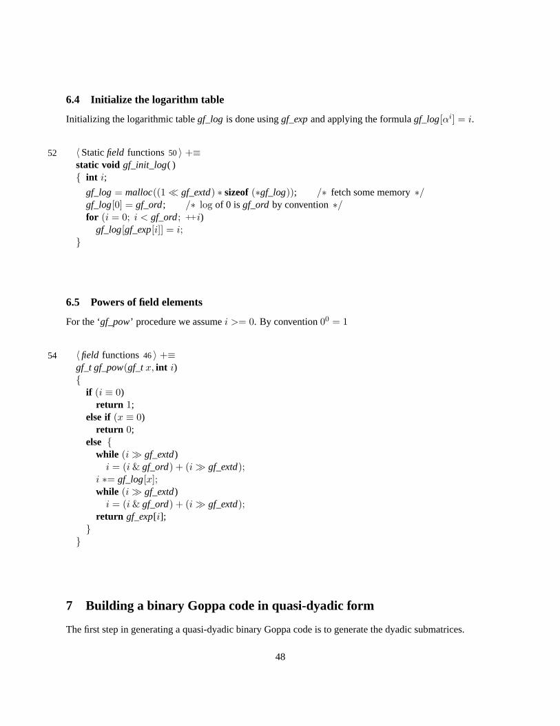
6.4 Initialize the logarithm table
Initializing the logarithmic tablegf_log is done usinggf_expand applying the formulagf_log[αi] = i.
〈Staticfield functions 50〉 +≡52static void gf_init_log( ){ int i;
gf_log= malloc((1≪ gf_extd) ∗ sizeof(∗gf_log)); /∗ fetch some memory∗/gf_log[0] = gf_ord; /∗ log of 0 isgf_ord by convention∗/for (i = 0; i < gf_ord; ++i)
gf_log[gf_exp[i]] = i;}
6.5 Powers of field elements
For the ‘gf_pow’ procedure we assumei >= 0. By convention00 = 1
〈 field functions 46〉 +≡54gf_t gf_pow(gf_tx, int i){
if (i ≡ 0)return 1;
else if (x ≡ 0)return 0;
else {while (i≫ gf_extd)i = (i& gf_ord) + (i≫ gf_extd);
i ∗= gf_log[x];while (i≫ gf_extd)i = (i& gf_ord) + (i≫ gf_extd);
return gf_exp[i];}}
7 Building a binary Goppa code in quasi-dyadic form
The first step in generating a quasi-dyadic binary Goppa code is to generate the dyadic submatrices.
48

7.1 Constructing a purely dyadic Goppa code
〈binary-quasi-dyadic-goppa-code.h 57〉 ≡57#ifndef BINARY_QD_GOPPA_CODE_H_INC#defineBINARY_QD_GOPPA_CODE_H_INC〈Exporteddyadicfunctions 58〉
#endif
〈Exporteddyadicfunctions 58〉 ≡58
void binary_quasi_dyadic_goppa_code(uint32_tm, uint32_tn, uint32_tt, int ∗b, gf_t ∗ h,gf_t ∗ omega, int ∗bc, int debug);
This code is used in section 57.
〈binary-quasi-dyadic-goppa-code.c 59〉 ≡59#include <stdio.h>#include <math.h>#include <stdlib.h>#include <string.h>#include "gf.h"#include "utils.h"〈Staticdyadicmacros60〉〈 dyadicfunctions 62〉
〈Staticdyadicmacros60〉 ≡60
#defineREMOVE_FROM_U(elt)for (int l = k; l < q; ++l) {
if (U [l] ≡ elt) {U [l] = 0;break;}}
See also section 61.
This code is used in section 59.
〈Staticdyadicmacros60〉 +≡61
#defineINIT_U_RANDOM( )U [0] = 0;for (int u = 1; u < q; ++u) {U [u] = gf_exp[u];}for (int u = 1; u < q − 1; ++u) {
register int v = (rand( ) % (u+ 1));
49

gf_ttmp= U [u];U [u] = U [v + 1];U [v + 1] = tmp;}
To construct a binary dyadic code, we follow the description as given in [4], Algorithm 2. The corre-sponding C code is given inbinary_quasi_dyadic_goppa_code. Inputs are the extension degreem, codelengthn, error capabilityt. Output is a dyadic signatureh, ω and the sequencebc of all consistent blocks ofcolumns. For simplicity, we use a codelengthn ≤ q/2 and a designed error numbert which is a power of2.
〈 dyadicfunctions 62〉 ≡62
void binary_quasi_dyadic_goppa_code(uint32_tm, uint32_tn, uint32_tt, int ∗b, gf_t ∗ h,gf_t ∗ omega, int ∗bc, int debug)
{ gf_t ∗ U ;
unsigned int c, k;int const q = 1≪ m;int const C = q/t;
〈Check ift is a power of2; exit in case it is not or in caset > (2m − 1)/m 63〉;〈 q ← 2m; exit in case code lengthn > q/2; initialize underlying field bufferU : U ← Fq \ {0} 64〉;〈Generate consistent root and support sets.65〉;〈 return h, bc andω. Free used buffer.74〉;}
This code is used in section 59.
〈Check ift is a power of2; exit in case it is not or in caset > (2m − 1)/m 63〉 ≡63
c = t; /∗ count the bits contained in t∗/c = (c& #55555555U) + ((c≫ 1) & #55555555U);c = (c& #33333333U) + ((c≫ 2) & #33333333U);c = (c& #0F0F0F0FU) + ((c≫ 4) & #0F0F0F0FU);c = (c& #00FF00FFU) + ((c≫ 8) & #00FF00FFU);c = (c& #0000FFFFU) + ((c≫ 16) & #0000FFFFU);if ((c 6= 1) ∨ (t ≡ 1) ∨ (t > 128) ∨ (t > ((double)(q − 1)/m))) {
fprintf (stderr,"ERROR t(%d) is not a power of 2 or bigger than %d\n", t, (q − 1)/m);exit(−1);}
This code is used in section 62.
To implement Algorithm2, we first initialize the field cardinality:q := 2m. In casen ≥ q, we print anerror message and exit. Otherwise we allocate memory for the underlying bufferU of the finite fieldFq.
〈 q ← 2m; exit in case code lengthn > q/2; initialize underlying field bufferU : U ← Fq \ {0} 64〉 ≡64
50

if (n > q/2) {fprintf (stderr,"ERROR n(%d) > q/2(%d)\n", n, q/2);exit(−1);}U = malloc(q ∗ sizeof(∗U));
This code is used in section 62.
In order to construct consistent root and support sets for the Goppapolynomial, the next step is to initializeU with the elements ofFq \ {0} and to pick randomly anh0 ∈ U . The remaining entries of the signaturehare determind inm steps. Per step, we generaten new entrieshn, where2s ≤ n < 2s+1 and0 ≤ s < m.It is possible that not all of thehn will receive a value different from zero. Depending on the number ofconsistent support blocks and the value oft, it might be necessary to re-initialize the field and to repeat thosem steps. However, the probability for this case is quite low.
After the signatureh has been calculated, we need to check its consistency. We also need to findaproperω to use in equation (2.4.45), theorem (2.4.34). To prevent spurious intersections between the rootset and the support set,ω has to be chosen with care. Firstly, resetU to Fq. While checking for the root andsupport set consistency, continuously remove elements out of those setsfrom U . ω can be chosen from theremainingU .
〈Generate consistent root and support sets.65〉 ≡65do {〈SetU ← Fq \ {0} 66〉;〈Seth0
$←U, U ← U \ {h0} 67〉;〈Determine the remaining signature entrieshn (1 ≤ n ≤ q − 1) 68〉;〈ResetU : U ← Fq for findingω 71〉;〈Check for consistent root and support set72〉;} while (c ∗ t < n);
This code is used in section 62.
InitializeU with the elements ofFq \ {0}. By construction, the exponential tablegf_expof the field doesnot contain zero, therefore we just copygf_expinto U . As the algorithm proceeds, used elements ofU willbe reset to zero. After the copy, both the first and the last position ofU contain1, soU [0] is not needed. BysettingU [0] to zero, it is marked as already used. Finally, entries ofU exceptU [0] are permuted randomly.
〈SetU ← Fq \ {0} 66〉 ≡66
srand((unsigned) rdtsc( ));〈ResetU : U ← Fq for findingω 71〉;
This code is used in section 65.
Since the entries aboveU [1] have been permuted randomly in the previous step, we just takeh0 := U [1].Removingh0 fromU is done by settingU [1] to zero.
〈Seth0$←U, U ← U \ {h0} 67〉 ≡67
h[0] = U [1];U [1] = 0;
This code is used in section 65.
51

In m steps, we determine thehn for 1 ≤ n < q. For each step, we update the read positionk, which meansthatU [n] = 0 for n < k. The value at the read position is taken to behi, wherei = 2s and0 ≤ s < m. Thehi+j , where1 ≤ j ≤ i− 1, are computed according to equation (2.4.45) in theorem (2.4.34).
〈Determine the remaining signature entrieshn (1 ≤ n ≤ q − 1) 68〉 ≡68
k = 1;for (int s = 0; s < m; ++s) {
while (U [k] ≡ 0 ∧ k < q − 1) /∗ move to the next read position∗/++k;
〈 i← 2s, hi$←U, U ← U \ {hi} 69〉
〈Generate nexthi+j for 1 ≤ j ≤ i− 1; U ← U \ {hi+j} 70〉}
This code is used in section 65.
Use forhi, i = 2s, the value at current read positionk, and delete the value ofhi fromU .
〈 i← 2s, hi$←U, U ← U \ {hi} 69〉 ≡69
int const i = 1≪ s;
h[i] = U [k];REMOVE_FROM_U(h[i]);
This code is used in section 68.
Oncehi is found, we calculate the value forhi+j , where1 ≤ j ≤ i − 1. To apply equation (2.4.45),theorem (2.4.34), we need to check forhi 6= 0, hj 6= 0 and1/hi + 1/hj + 1/h0 6= 0. In case all threechecks succeed, we sethi+j = 1/(1/hi + 1/hj + 1/h0) and remove its value fromU . Otherwise,hi+j isan undefined entry and set to zero.
〈Generate nexthi+j for 1 ≤ j ≤ i− 1; U ← U \ {hi+j} 70〉 ≡70
for (int j = 1; j < i; ++j) {h[i+ j] = 0;if (h[i] ∧ h[j]) {h[i+ j] = gf_add(gf_inv(h[i]), gf_inv(h[j]));h[i+ j] = gf_add(h[i+ j], gf_inv(h[0]));}if (h[i+ j]) {h[i+ j] = gf_inv(h[i+ j]);REMOVE_FROM_U(h[i+ j]);} else if (debug≥ 5)
fprintf (stderr,"INFO: undefined entry at %d\n", i+ j);}
This code is used in section 68.
〈ResetU : U ← Fq for findingω 71〉 ≡71
INIT_U_RANDOM( );This code is used in sections 65, 66, and 72.
52

Theorem (2.4.34) shows that the root set is consistent, if0 /∈ {h0, . . . , ht−1}, and that elementszi of theroot set are defined aszi = 1/hi, 0 ≤ i ≤ t− 1. If the root set is consistent, allzi will be removed fromU .To prevent spurios intersections between the root setz and the support setL, we also remove the elementsof the form1/hi + 1/h0. Finally, check for consistent support blocks.
〈Check for consistent root and support set72〉 ≡72
c = 0;
int consistent_root_set= 1;
for (int i = 0; i < t; ++i)consistent_root_set&= (h[i] 6= 0);
if (consistent_root_set) {k = 1;memset(b, #00, C ∗ sizeof(∗b));〈ResetU : U ← Fq for findingω 71〉b[0] = 0;c = 1;REMOVE_FROM_U(gf_inv(h[0]));for (int i = 1; i < t; ++i) {REMOVE_FROM_U(gf_add(gf_inv(h[i]), gf_inv(h[0])));REMOVE_FROM_U(gf_inv(h[i]));}〈Determine consistent support blocks{hjt, . . . , h(j+1)t−1} 73〉}
This code is used in section 65.
As with the root set, a support block is consistent if0 /∈ {hjt, . . . , h(j+1)t−1} for 1 ≤ j ≤ ⌊q/t⌋, inwhich case we remove the corresponding elements fromU . According to theorem (2.4.34), those elementare characterized by{1/hi + 1/h0 | i = jt, . . . , (j + 1)t − 1}, where1 ≤ j ≤ ⌊q/t⌋. The positions of theconsistent blocks is saved for later use.
〈Determine consistent support blocks{hjt, . . . , h(j+1)t−1} 73〉 ≡73
for (int j = 1; j < C; ++j) {while (U [k] ≡ 0 ∧ k < q − 1) ++k;
int consistent_support_block= 1;
for (int i = j ∗ t; i < (j + 1) ∗ t; ++i) consistent_support_block&= (h[i] 6= 0);if (consistent_support_block) {b[c] = j;++c;for (int i = j ∗ t; i < (j + 1) ∗ t; ++i) {REMOVE_FROM_U(gf_add(gf_inv(h[i]), gf_inv(h[0])));}}}
This code is used in section 72.
53
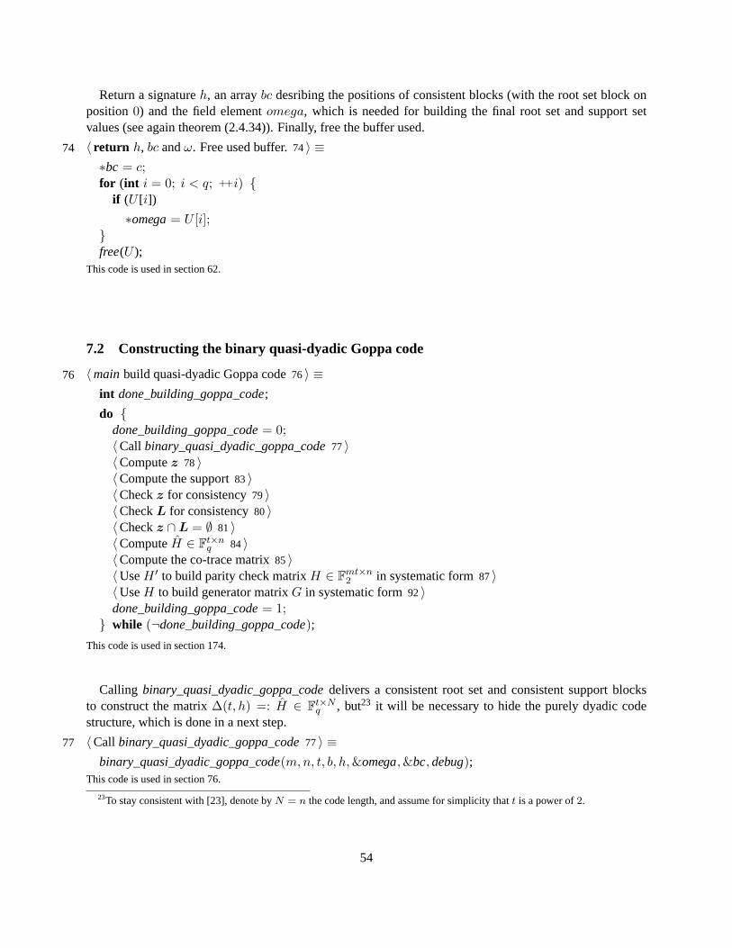
Return a signatureh, an arraybc desribing the positions of consistent blocks (with the root set block onposition0) and the field elementomega, which is needed for building the final root set and support setvalues (see again theorem (2.4.34)). Finally, free the buffer used.
〈 return h, bc andω. Free used buffer.74〉 ≡74
∗bc = c;for (int i = 0; i < q; ++i) {
if (U [i])
∗omega= U [i];}free(U );
This code is used in section 62.
7.2 Constructing the binary quasi-dyadic Goppa code
〈mainbuild quasi-dyadic Goppa code76〉 ≡76
int done_building_goppa_code;
do {done_building_goppa_code= 0;〈Call binary_quasi_dyadic_goppa_code77〉〈Computez 78〉〈Compute the support83〉〈Checkz for consistency79〉〈CheckL for consistency80〉〈Checkz ∩L = ∅ 81〉〈ComputeH ∈ F
t×nq 84〉
〈Compute the co-trace matrix85〉〈UseH ′ to build parity check matrixH ∈ F
mt×n2 in systematic form87〉
〈UseH to build generator matrixG in systematic form92〉done_building_goppa_code= 1;} while (¬done_building_goppa_code);
This code is used in section 174.
Calling binary_quasi_dyadic_goppa_codedelivers a consistent root set and consistent support blocksto construct the matrix∆(t, h) =: H ∈ F
t×Nq , but23 it will be necessary to hide the purely dyadic code
structure, which is done in a next step.
〈Call binary_quasi_dyadic_goppa_code77〉 ≡77
binary_quasi_dyadic_goppa_code(m,n, t, b, h,&omega,&bc, debug);This code is used in section 76.
23To stay consistent with [23], denote byN = n the code length, and assume for simplicity thatt is a power of2.
54

As given in theorem (2.4.34), we havezi := 1/hi + ω.
〈Computez 78〉 ≡78for (int i = 0; i < t; ++i) {z[i] = gf_add(gf_inv(h[i]), omega);if (debug≥ 3)
printf ("z[%d] = %04x\n", i, z[i]);}
This code is used in section 76.
〈Checkz for consistency79〉 ≡79
for (int i = 0; i < t; ++i)for (int j = 0; j < t; ++j)
if ((i 6= j) ∧ (z[i] ≡ z[j])) {fprintf (stderr,"ERROR: z[%d]=%04x == z[%d]=%04x\n", i, z[i], j, L[j]);continue;}
This code is used in section 76.
〈CheckL for consistency80〉 ≡80
for (int i = 0; i < n; ++i)for (int j = 0; j < n; ++j)
if ((i 6= j) ∧ (L[i] ≡ L[j])) {fprintf (stderr,"ERROR: L[%d]=%04x == L[%d]=%04x\n", i, L[i], j, L[j]);continue;}
This code is used in section 76.
〈Checkz ∩L = ∅ 81〉 ≡81
for (int i = 0; i < t; ++i)for (int j = 0; j < n; ++j)
if (z[i] ≡ L[j]) {fprintf (stderr,"ERROR: z[%d]=%04x == L[%d]=%04x\n", i, z[i], j, L[j]);continue;}
This code is used in section 76.
∆(t, h) = H ∈ Ft×Nq can be seen as an array ofN/t dyadic blocks of sizet×t: H =
[
B0 . . . BN/t−1
]
,
whereB0 = ∆(h0, . . . , ht−1) is the root block. The calculation of the rootszi of the Goppa polynomialg(X) ∈ Fq[X] is done as prescribed by theorem (2.4.34):
zi := 1/hi + ω,
g(X) :=t−1∏
i=0
(X − zi).
55

〈mainassemble the Goppa polynomial82〉 ≡82
g = poly_alloc(1);poly_set_coeff(g, 0, z[0]);poly_set_coeff(g, 1, 1);poly_calcule_deg(g);poly_tp = poly_copy(g);poly_calcule_deg(p);for (int i = 1; i < t; ++i) {
poly_set_coeff(p, 0, z[i]);poly_t p_old= g;g = poly_mul(g, p);poly_free(p_old);}poly_free(p);poly_calcule_deg(g);g2 = poly_mul(g, g);
This code is used in section 174.
Using the consistent root set and consistent support blocks, the support L is again computed using theo-rem (2.4.34):
Lj = 1/hj + 1/h0 + ω.
〈Compute the support83〉 ≡83
for (int j = 0, k = 0; k < bc; ++k) {for (int i = 0; i < t; ++i) {
if (j < n) {gf_t a0= gf_inv(h[0]);a0 = gf_add(a0, omega);gf_t a1= gf_inv(h[b[k] ∗ t+ i]);L[j] = gf_add(a0, a1);if (debug≥ 3)
printf ("L[%d] = %04x\n", j, L[j]);++j;
}}}
This code is used in section 76.
〈ComputeH ∈ Ft×nq 84〉 ≡84
for (int i = 0; i < t; ++i)for (int j = 0; j < n; ++j)H[i ∗ n+ j] = gf_inv(gf_add(z[i], L[j]));
This code is used in section 76.
56

〈Compute the co-trace matrix85〉 ≡85
if (Hbin 6= Λ) mat_free(Hbin);Hbin = mat_ini(m ∗ t, n);if (Hbin ≡ Λ) {
fprintf (stderr,"INFO: mat_ini failed\n");continue;}mat_set_to_zero(Hbin);for (int i = 0; i < n; i++)
for (int j = 0; j < t; j++) {constgf_ty = H[j ∗ n+ i];
for (int k = 0; k < m; k++) {if (y & (1≪ k)) {
const int idx = (t ∗ k + j) ∗ Hbin~ rwdcnt+ i/BITS_PER_LONG;
Hbin~ elem[idx] ⊕= (1U L ≪ (i %BITS_PER_LONG));}}}
if (debug≥ 5)〈Print co-traced matrix86〉
This code is used in section 76.
〈Print co-traced matrix86〉 ≡86print_bin_matrix(m ∗ t, n,Hbin,"Hbin AFTER CO-TRACING:");
This code is used in section 85.
To transformHbin into systematic form, theHyMES function mat_rref is used. Because it is possiblethat a co-traced matrix does not have the full rankn−mt, an explicit check is necessary.
〈UseH ′ to build parity check matrixH ∈ Fmt×n2 in systematic form87〉 ≡87
int ∗perm= mat_rref(Hbin);
if (perm≡ Λ) {if (debug≥ 5)
fprintf (stderr,"INFO: mat_rref FAILED FOR Hbin\n");continue;}free(perm); /∗ permutation not used∗/int Hbin_in_systematic_form= 1;〈Check Hbin for systematic form88〉
if (Hbin_in_systematic_form)〈Change row order89〉
else {if (debug≥ 5)
fprintf (stderr,"INFO: co-traced matrix not of full rank.\n");
57
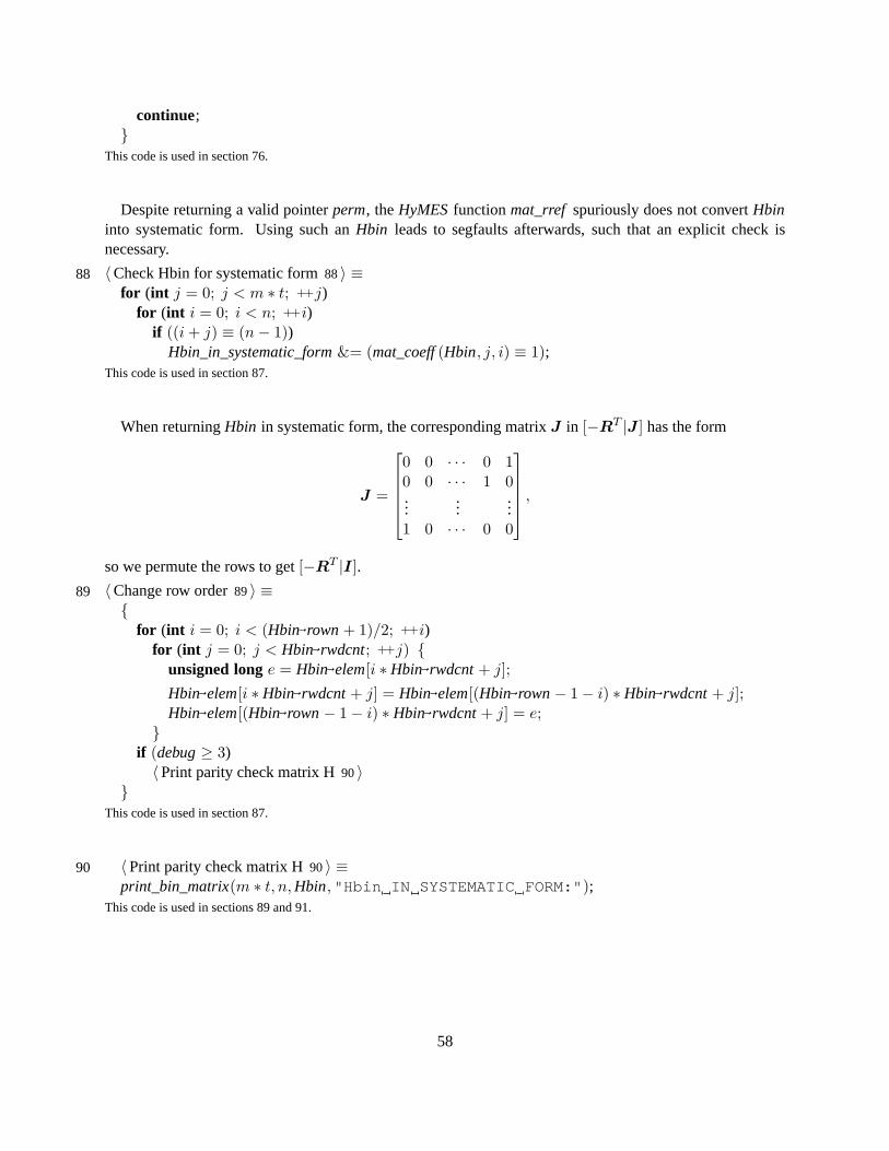
continue;}
This code is used in section 76.
Despite returning a valid pointerperm, theHyMESfunctionmat_rref spuriously does not convertHbininto systematic form. Using such anHbin leads to segfaults afterwards, such that an explicit check isnecessary.
〈Check Hbin for systematic form88〉 ≡88for (int j = 0; j < m ∗ t; ++j)
for (int i = 0; i < n; ++i)if ((i+ j) ≡ (n− 1))
Hbin_in_systematic_form&= (mat_coeff(Hbin, j, i) ≡ 1);This code is used in section 87.
When returningHbin in systematic form, the corresponding matrixJ in [−RT |J ] has the form
J =
0 0 · · · 0 10 0 · · · 1 0...
......
1 0 · · · 0 0
,
so we permute the rows to get[−RT |I].〈Change row order89〉 ≡89{
for (int i = 0; i < (Hbin~ rown+ 1)/2; ++i)for (int j = 0; j < Hbin~ rwdcnt; ++j) {
unsigned longe = Hbin~ elem[i ∗ Hbin~ rwdcnt+ j];
Hbin~ elem[i ∗ Hbin~ rwdcnt+ j] = Hbin~ elem[(Hbin~ rown− 1− i) ∗ Hbin~ rwdcnt+ j];Hbin~ elem[(Hbin~ rown− 1− i) ∗ Hbin~ rwdcnt+ j] = e;}
if (debug≥ 3)〈Print parity check matrix H90〉
}This code is used in section 87.
〈Print parity check matrix H90〉 ≡90print_bin_matrix(m ∗ t, n,Hbin,"Hbin IN SYSTEMATIC FORM:");
This code is used in sections 89 and 91.
58

〈CheckGHT = 0 91〉 ≡91for (int i = 0; i < n−m ∗ t; ++i)
for (int k = 0; k < m ∗ t; ++k) {int x = 0;
for (int j = 0; j < n; ++j)x += mat_coeff(Gbin, i, j) ∗mat_coeff(Hbin, k, j);
if (x& 1) {fprintf (stderr,"ERROR: GH^T != 0 (%d,%d)\n", i, k);〈Print parity check matrix H90〉〈Print generator matrix G93〉i = n−m ∗ t;k = m ∗ t;continue;}}
This code is used in section 92.
As the parity check matrix has formH = [RT |In−mt] ∈ F(n−mt)×n2 , the public generator matrix in
systematic form has formG = [Imt|R] ∈ Fmt×n2 . The redundant partR ∈ F
mt×(n−mt)2 is a quasi-dyadic
matrix.
〈UseH to build generator matrixG in systematic form92〉 ≡92
if (Gbin 6= Λ) mat_free(Gbin);Gbin = mat_ini(n−m ∗ t, n); /∗ n-mt = k ∗/if (Gbin 6= Λ) {
mat_set_to_zero(Gbin);for (int i = 0; i < n−m ∗ t; ++i)
for (int j = 0; j < n; ++j)if (i ≡ j)
mat_set_coeff_to_one(Gbin, i, j);elseif (j ≥ n−m ∗ t)
if (mat_coeff(Hbin, j − n+m ∗ t, i))mat_set_coeff_to_one(Gbin, i, j);
〈CheckGHT = 0 91〉;if (debug≥ 3)〈Print generator matrix G93〉;
}else {
fprintf (stderr,"INFO: mat_ini FAILED FOR Gbin\n");continue;}
This code is used in section 76.
〈Print generator matrix G93〉 ≡93print_bin_matrix(n−m ∗ t, n,Gbin,"Gbin IN SYSTEMATIC FORM:");
This code is used in sections 91, 92, and 183.
59

8 The encryption step
8.1 The fast Walsh-Hadamard transform (FWHT) and the dyadic convolution
As noted in section (2.4.8), remark (2.4.43) provides an efficient way to perform a vector-matrix product inthe form ofuHk for u ∈ F
r. The algorithm is shown infwht. For the purposes of this thesis, a datatypeof int provides enough space for the lifting toZ. In case the datatype has to be extended,fwht will be morecomplicated as well.
Besidesfwht, a more direct way to computeuHk is given with thevm-functions (see section (8.1.2)).Although onlyvm4is used in the actual implementation, other versions for other datatypes are given as wellto clarify the pattern underlying thevm-functions.
〈fwht.h 96〉 ≡96#ifndef FWHT_H_INCLUDED#defineFWHT_H_INCLUDED#include <inttypes.h>
typedef int fwht t ;
extern fwht t ∗fwht(unsignedk, fwht t ∗u);extern uint8_t vm4(uint8_tv, uint8_tm);extern uint8_t vm2x4(uint8_tv, uint8_tm);extern uint8_t vm8(uint8_tv, uint8_tm);extern uint16 t vm16(uint16 t v, uint16 t m);extern uint32_t vm32(uint32_tv, uint32_tm);
#endif
8.1.1 uHk via the fast Walsh-Hadamard transform
〈fwht.c 98〉 ≡98#include <stdio.h>#include <stdlib.h>#include "fwht.h"〈 fwht functions 99〉
The fastWalsh− Hadamard transformtakes as inputk ∈ N, u ∈ Fr with r = 2k and is done in
characteristic6= 2. fwht is a straight-forward implementation of (2.4.49).
〈 fwht functions 99〉 ≡99
60

fwht t ∗fwht(unsignedk, fwht t ∗u){
register unsigned constr = (1≪ k);register unsignedi, j, h, s = k + 1;register unsignedd = 1;
while (−−s) {h = d;d≪= 1;for (i = 0; i < r; i += d) {
for (j = 0; j < h; ++j) {register fwht t ∗p = u+ i+ j;register fwht t ∗q = u+ i+ j + h;register fwht t const v = ∗p;register fwht t constw = ∗q;∗p = v + w;∗q = v − w;
}}}return u;}
See also sections 101, 102, 103, and 104.
This code is used in section 98.
8.1.2 uHk directly via vm-functions
To illustrate the idea of thevm-functions, consider the dyadic matrixHk with k = 8:
Hk =
A B C D E F G HB A D C F E H GC D A B G H E FD C B A H G F EE F G H A B C DF E H G B A D CG H E F C D A BH G F E D C B A
.
If we interpret the characters as bits, we see that the second row is the first one, where the bits have beenswapped. The third row is like the first one, where nyps24 have been swapped. The fourth one is like thethird one, where the bits have been swapped. Finally, the fifth row is again like the first one, where nybbles25
have been swapped, and all the previous steps are repeated.
24Groups of two bits.25Groups of four bits.
61

To compute the productuHk we store the current row. In case the corresponding bit is set inu, thecurrent row is added to the end result. The same pattern applies for the other vm-functions. The onlydifference is how much must be swapped when crossing the(n/2).th row.
〈 fwht functions 99〉 +≡101
uint8_t vm8(uint8_tv, uint8_tm){
int i;
uint8_t res= 0;for (i = 0; i < 8; ++i) {
int n = i;
uint8_tr = m; /∗ save signature in r∗/if (n ≥ 4) {r = (((r & #0F)≪ 4) | ((r & #F0)≫ 4)); /∗ swap nybbles∗/n = n− 4;}if (n ≥ 2) {r = (((r & #33)≪ 2) | ((r & #CC)≫ 2)); /∗ swap nyps∗/n = n− 2;}if (n ≡ 1) {r = (((r & #55)≪ 1) | ((r & #AA)≫ 1)); /∗ swap bits∗/}if ((v ≫ (7− i)) & 1) { /∗bitsetinv, addrow ∗/
res= res⊕ r;}}return res;}
〈 fwht functions 99〉 +≡102
uint8_t vm4(uint8_tv, uint8_tm){
int i;
uint8_t res= 0;for (i = 0; i < 4; ++i) {
int n = i;
uint8_t row= m;if (n ≥ 2) {
row = (((row & #33)≪ 2) | ((row & #CC)≫ 2)); /∗ swap nyps∗/n = n− 2;}if (n ≡ 1) {
row = (((row & #55)≪ 1) | ((row & #AA)≫ 1)); /∗ swap bits∗/
62

}if ((v ≫ (3− i)) & 1) {
res= res⊕ row;}}return res;}
〈 fwht functions 99〉 +≡103
uint16 t vm16(uint16 t v, uint16 t m){
int i;uint16 t res= 0;
for (i = 0; i < 16; ++i) {int n = i;uint16 t r = m;
if (n ≥ 8) {r = (((r & #00FF)≪ 8) | ((r & #FF00)≫ 8)); /∗ swap bytes∗/n = n− 8;}if (n ≥ 4) {r = (((r & #0F0F)≪ 4) | ((r & #F0F0)≫ 4)); /∗ swap nybbles∗/n = n− 4;}if (n ≥ 2) {r = (((r & #3333)≪ 2) | ((r & #CCCC)≫ 2)); /∗ swap nyps∗/n = n− 2;}if (n ≡ 1) {r = (((r & #5555)≪ 1) | ((r & #AAAA)≫ 1)); /∗ swap bits∗/}if ((v ≫ (15− i)) & 1) {
res= res⊕ r;}}return res;}
〈 fwht functions 99〉 +≡104
uint32_t vm32(uint32_tv, uint32_tm){
int i;
63

uint32_t res= 0;for (i = 0; i < 32; ++i) {
int n = i;
uint32_tr = m;if (n ≥ 16) {r = (((r & #0000FFFF)≪ 16) | ((r & #FFFF0000)≫ 16)); /∗ swap half words∗/n = n− 16;}if (n ≥ 8) {r = (((r & #00FF00FF)≪ 8) | ((r & #FF00FF00)≫ 8)); /∗ swap bytes∗/n = n− 8;}if (n ≥ 4) {r = (((r & #0F0F0F0F)≪ 4) | ((r & #F0F0F0F0)≫ 4)); /∗ swap nybbles∗/n = n− 4;}if (n ≥ 2) {r = (((r & #33333333)≪ 2) | ((r & #CCCCCCCC)≫ 2)); /∗ swap nyps∗/n = n− 2;}if (n ≡ 1) {r = (((r & #55555555)≪ 1) | ((r & #AAAAAAAA)≫ 1)); /∗ swap bits∗/}if ((v ≫ (31− i)) & 1) {
res= res⊕ r;}}return res;}
8.1.3 The dyadic convolution
Let∆(u) and∆(v) dyadic matrices. Then the dyadic convolution computes∆(w) = ∆(u)∆(v) using thesignaturesu andv only. There is no need to unfold the dyadic matrices in memory.
〈dyadic-convolution.h 106〉 ≡106#ifndef DYADIC_CONVOLUTION_H_INCLUDED#defineDYADIC_CONVOLUTION_H_INCLUDED#include "fwht.h"
extern fwht t ∗dyadic_conv(unsignedk, fwht t ∗u, fwht t ∗v);#endif
64

〈dyadic-convolution.c 107〉 ≡107#include "dyadic-convolution.h"〈 dyadic convolutionfunctions 108〉
The input for the dyadic convolution isk ∈ N, u,v ∈ Fr with r = 2k and char(F) 6= 2. The output is
w ∈ Fr such that∆(w) = ∆(u)∆(v).
〈 dyadic convolutionfunctions 108〉 ≡108
fwht t ∗dyadic_conv(unsignedk, fwht t ∗u, fwht t ∗v){
register fwht t const ∗constr = &u[1≪ k];register fwht t ∗p = fwht(k, u); /∗ computeu = uHk via FWHT∗/register fwht t ∗q = fwht(k, v); /∗ computev = vHk via FWHT∗/while (p < r) { /∗ wi = uivi ∗/∗p ∗= ∗q;++p;++q;
}p = fwht(k, u); /∗ computew = wHk via FWHT∗/while (p < r) { /∗w = 2−kw ∗/∗p≫= k;++p;
}return u; /∗ return w ∗/}
This code is used in section 107.
9 The decryption step
The original McEliece scheme was based on binary irreducible Goppa codes. An efficient decoder forcodes of this kind is based on Patterson’s algorithm [24]. However, forseparable binary Goppa codesPatterson’s algorithm is not directly usable, and only recently a generalization of Patterson’s algorithm hasbeen published [5]26. Because Goppa codes are special alternant codes, alternant decoders can be used todecode them. The classical decoder presented now turns out to be slower slower than Patterson’s, but it isstill in widespread use. As MacWilliams and Sloane quote ([20], p. 369):
"Nevertheless, decoding using the Euclidean algorithm is by far the simplest tounderstand, and is cer-tainly at least comparable in speed with the other methods (forn < 106) and so it is the method we prefer."
The following exposition is according to [20, 26].
26Which is beyond the scope of this thesis.
65

〈alternant-decode.h 110〉 ≡110#ifndef ALTERNANT_DECODE_H_INCLUDED#defineALTERNANT_DECODE_H_INCLUDED#include "gf.h"#include "poly.h"
extern gf_t∗cons_parity_check(int n, int t, poly_t g2, constgf_t∗L, int debug);extern poly_t cons_syndrome_polynomial(int n, int tt, constgf_t∗cw, constgf_t∗H2T);extern void solve_key_equation(poly_t ∗ sigma, poly_t ∗ omega, poly_tS, poly_t g2, int t);
#endif
〈alternant-decode.c 111〉 ≡111#include <stdio.h>#include <math.h>#include <stdlib.h>#include <string.h>#include "alternant-decode.h"#include "utils.h"〈 decodefunctions 113〉
9.1 The setup
Construct the parity check matrix as desribed in (5.1.3). Inputs are the dimensionsn and2t, the square ofthe Goppa polynomialg(X) and the supportL. Output isH ′ ≡H2T .
〈 decodefunctions 113〉 ≡113
gf_t ∗ cons_parity_check(int n, int tt, poly_t g2, constgf_t∗L, int debug){
gf_te[n], c[n];gf_t ∗ H2 = calloc(tt ∗ n, sizeof(∗H2));gf_t ∗ H2T = calloc(tt ∗ n, sizeof(∗H2T));if (H2 ∧ H2T) {
for (int j = 0; j < n; ++j) {e[j] = poly_eval(g2, L[j]);e[j] = gf_inv(e[j]);c[j] = 0;}for (int i = 0; i < tt; ++i) {
for (int j = 0; j < n; ++j) {c[j] = gf_mul(c[j], L[j]);c[j] = gf_add(c[j], poly_coeff(g2, tt − i));
}for (int j = 0; j < n; ++j)
66

H2[i ∗ n+ j] = gf_mul(e[j], c[j]);}for (int i = 0; i < tt; ++i)
for (int j = 0; j < n; ++j)H2T[j ∗ tt + i] = H2[i ∗ n+ j];
free(H2);if (debug≥ 3) {〈Print parity check H2T114〉;}}return H2T;}
See also sections 116 and 118.
This code is used in section 111.
〈Print parity check H2T114〉 ≡114print_matrix(tt, n,H2T,"H2T");
This code is used in section 113.
Call cons_parity_checkin themain function.
〈mainconstruct parity check matrixH2T for the private decoder115〉 ≡115H2T = cons_parity_check(n, 2 ∗ t, g2, L, debug);
This code is used in section 174.
9.2 Construct the syndrome polynomial
The syndrome polynomial of a received vectoru ∈ Fn2 can be computed either directly using the definition,
S(X) ≡n−1∑
i=0
uiX − Li
≡n−1∑
i=0
eiX − Li
mod g(X)
or, as we do, using the canonical parity check matrixH, see (2.4.26). The received vectoru has to bemultiplied from the left ontoHT ∈ F
n×2t2m ,
uHT = [S2t−1, . . . , S0] (9.2.1)
where theSi with 0 ≤ i ≤ 2t− 1 represent the coefficients of the syndrome polynomial.
〈 decodefunctions 113〉 +≡116
poly_t cons_syndrome_polynomial(int n, int tt, constgf_t∗u, constgf_t∗H2T){ gf_ts[tt];
poly_tS = poly_alloc(tt − 1);
67

for (int i = 0; i < tt; ++i)s[i] = 0;
for (int i = 0; i < tt; ++i)for (int j = 0; j < n; ++j) {
gf_tc = gf_mul(u[j],H2T[j ∗ tt + i]);s[i] = gf_add(s[i], c);}
for (int i = 0; i < tt; ++i)poly_set_coeff(S, tt − 1− i, s[i]);
poly_calcule_deg(S);return S;}
〈maincompute the syndrome polynomial117〉 ≡117SyM= cons_syndrome_polynomial(n, 2 ∗ t, cw,H2T);
This code is used in section 185.
9.3 Solve the key equation
ω(X) ≡ σ(X)S(X) mod g(X)
〈 decodefunctions 113〉 +≡118
void solve_key_equation(poly_t ∗ poly_sigma, poly_t ∗ poly_omega, poly_tS, poly_t g2, int t){
poly_eeaux(poly_sigma, poly_omega, S, g2, t);}
〈mainsolve the key equationω(X) = σ(X)S(X) mod g(X) 119〉 ≡119
solve_key_equation(&poly_sigma,&poly_omega,SyM, g2, t);This code is used in section 185.
9.4 Find the error positions and correct codeword
Finding and correcting the error positions as done in themain function using the supportL. Note thatin general much more sophisticated methods are deployed like Chien search [9] or Berlekamp’s trace algo-rithm [7].
68

〈maincorrect errors121〉 ≡121poly_calcule_deg(poly_sigma);poly_calcule_deg(poly_omega);for (int i = 0; i < n; ++i)
if (poly_eval(poly_sigma, L[i]) ≡ 0)cw[i] = (cw[i] ≡ 1) ? 0 : 1;
This code is used in section 185.
10 Additional source code
Sections (10.1) and (10.2) are taken from HyMES [29] with minor corrections.
10.1 Polynomials
〈poly.h 124〉 ≡124#ifndef POLY_H_INCLUDED#definePOLY_H_INCLUDED
typedef struct polynome{int deg;int size;
gf_t ∗ coeff;} ∗poly t ;
#definepoly_deg(p) ((p)~ deg)#definepoly_size(p) ((p)~ size)#definepoly_set_deg(p, d) ((p)~ deg= (d))#definepoly_coeff(p, i) ((p)~ coeff[i])#definepoly_set_coeff(p, i, a) ((p)~ coeff[i] = (a))#definepoly_addto_coeff(p, i, a) ((p)~ coeff[i] = gf_add((p)~ coeff[i], (a)))#definepoly_multo_coeff(p, i, a) ((p)~ coeff[i] = gf_mul((p)~ coeff[i], (a)))#definepoly_tete(p) ((p)~ coeff[(p)~ deg])
extern int poly_calcule_deg(poly t p);extern void poly_set(poly t p, poly t q);extern void poly_set_to_zero(poly t p);extern poly t poly_alloc(int d);extern poly t poly_copy(poly t p);extern void poly_free(poly t p);extern poly t poly_mul(poly t p, poly t q);extern gf_t poly_eval(poly t p, gf_ta);extern void poly_eeaux(poly t ∗u, poly t ∗v, poly t p, poly t g, int t);
#endif
69

〈poly.c 125〉 ≡125#include <stdio.h>#include <stdlib.h>#include <string.h>#include "gf.h"#include "poly.h"〈Staticpoly functions 133〉〈Exportedpoly functions 126〉
〈Exportedpoly functions 126〉 ≡126
poly t poly_alloc(int d) { poly t p;
p = (poly t ) malloc(sizeof(struct polynome));p~ deg= −1;p~ size= d+ 1; p~ coeff = ( gf_t ∗ ) calloc(p~ size, sizeof(gf_t));return p; }
See also sections 127, 128, 129, 130, 131, 132, 134, and 135.
This code is used in section 125.
〈Exportedpoly functions 126〉 +≡127
void poly_free(poly t p){
free(p~ coeff);free(p);}
〈Exportedpoly functions 126〉 +≡128
void poly_set(poly t p, poly t q){ /∗ copy q in p∗/
int d = p~ size− q~ size;
if (d < 0) {memcpy(p~ coeff, q~ coeff, p~ size∗ sizeof(gf_t));poly_calcule_deg(p);}else {
memcpy(p~ coeff, q~ coeff, q~ size∗ sizeof(gf_t));memset(p~ coeff+ q~ size, 0, d ∗ sizeof(gf_t));p~ deg= q~ deg;}}
70

〈Exportedpoly functions 126〉 +≡129
void poly_set_to_zero(poly t p){
memset(p~ coeff, 0, p~ size∗ sizeof(gf_t));p~ deg= −1;}
〈Exportedpoly functions 126〉 +≡130
poly t poly_copy(poly t p) { poly t q;
q = (poly t ) malloc(sizeof(struct polynome));q~ deg= p~ deg;q~ size= p~ size; q~ coeff = ( gf_t ∗ ) calloc(q~ size, sizeof(gf_t));memcpy(q~ coeff, p~ coeff, p~ size∗ sizeof(gf_t));return q; }
〈Exportedpoly functions 126〉 +≡131
int poly_calcule_deg(poly t p){
int d = p~ size− 1;
while ((d ≥ 0) ∧ (p~ coeff[d] ≡ gf_zero( ))) −−d;p~ deg= d;return d;}
〈Exportedpoly functions 126〉 +≡132
poly t poly_mul(poly t p, poly t q){
int i, j, dp, dq;poly t r;
poly_calcule_deg(p);poly_calcule_deg(q);dp = poly_deg(p);dq = poly_deg(q);r = poly_alloc(dp+ dq);for (i = 0; i ≤ dp; ++i)
for (j = 0; j ≤ dq; ++j) poly_addto_coeff(r, i+ j, gf_mul(poly_coeff(p, i), poly_coeff(q, j)));poly_calcule_deg(r);return (r);}
71

〈Staticpoly functions 133〉 ≡133
gf_t poly_eval_aux(gf_t ∗ coeff, gf_ta, int d){
gf_tb;b = coeff[d−−];for ( ; d ≥ 0; −−d)
if (b 6= gf_zero( )) b = gf_add(gf_mul(b, a), coeff[d]);else b = coeff[d];
return b;}
This code is used in section 125.
〈Exportedpoly functions 126〉 +≡134
gf_t poly_eval(poly t p, gf_ta){
return poly_eval_aux(p~ coeff, a, poly_deg(p));}
The extended Euclidean algorithm. General assumption:deg g ≥ deg p.
〈Exportedpoly functions 126〉 +≡135
void poly_eeaux(poly t ∗u, poly t ∗v, poly t p, poly t g, int t){
int i, j, dr, du, delta;
gf_ta;
poly t aux, r0, r1, u0, u1;
dr = poly_deg(g); /∗ r0 := g, r1 := p, u0 := 0, u1 := 1 ∗/r0 = poly_alloc(dr);r1 = poly_alloc(dr − 1);u0 = poly_alloc(dr − 1);u1 = poly_alloc(dr − 1);poly_set(r0, g);poly_set(r1, p);poly_set_to_zero(u0);poly_set_to_zero(u1);poly_set_coeff(u1, 0, gf_unit( ));poly_set_deg(u1, 0);
/∗ invariants:r1 = u1 ∗ p+ v1 ∗ gr0 = u0 ∗ p+ v0 ∗ g anddeg u1 = deg g − deg r0. It stopswhendeg r1 < t (deg r0 ≥ t). And thereforedeg u1 = deg g − deg r0 < deg g − t ∗/
du = 0;dr = poly_deg(r1);delta= poly_deg(r0)− dr;while (dr ≥ t) {
for (j = delta; j ≥ 0; −−j) {
72

a = gf_div(poly_coeff(r0, dr + j), poly_coeff(r1, dr));if (a 6= gf_zero( )) { /∗ u0(z) <- u0(z) + a * u1(z) *zj ∗/
for (i = 0; i ≤ du; ++i) {poly_addto_coeff(u0, i+ j, gf_mul_fast(a, poly_coeff(u1, i)));} /∗ r0(z) <- r0(z) + a * r1(z) *zj ∗/for (i = 0; i ≤ dr; ++i) poly_addto_coeff(r0, i+ j, gf_mul_fast(a, poly_coeff(r1, i)));
}} /∗ exchange∗/aux= r0;r0 = r1;r1 = aux;aux= u0;u0 = u1;u1 = aux;du = du+ delta;delta= 1;while (poly_coeff(r1, dr − delta) ≡ gf_zero( )) delta++;dr −= delta;}poly_set_deg(u1, du);poly_set_deg(r1, dr); /∗ return u1 and r1;∗/∗u = u1;∗v = r1;poly_free(r0);poly_free(u0);}
10.2 Matrix functions
〈matrix.h 137〉 ≡137#ifndef MATRIX_H_INCLUDED#defineMATRIX_H_INCLUDED
#defineBITS_PER_LONG (8 ∗ sizeof(unsigned long))#definemat_coeff(A, i, j)(((A)~ elem[(i) ∗A~ rwdcnt+ (j)/BITS_PER_LONG]≫ (j %BITS_PER_LONG)) & 1)
#definemat_set_coeff_to_one(A, i, j)((A)~ elem[(i) ∗A~ rwdcnt+ (j)/BITS_PER_LONG] |= (1U L ≪ ((j) %BITS_PER_LONG)))
#definemat_change_coeff(A, i, j)((A)~ elem[(i) ∗A~ rwdcnt+ (j)/BITS_PER_LONG] ⊕= (1U L ≪ ((j) %BITS_PER_LONG)))
#definemat_set_to_zero(R)memset((R)~ elem, 0, (R)~ alloc_size);
typedef struct matrix {int rown; /∗ number of rows∗/int coln; /∗ number of columns∗/
73

int rwdcnt; /∗ number of words in a row∗/int alloc_size; /∗ number of allocated bytes∗/unsigned long∗elem; /∗ row index ∗/} ∗binmat t ;
extern binmat t mat_ini(int rown, int coln);extern binmat t mat_ini_from_string(int rown, int coln, const unsigned char∗s);extern void mat_free(binmat t A);extern binmat t mat_copy(binmat t A);extern binmat t mat_rowxor(binmat t A, int a, int b);extern int ∗mat_rref(binmat t A);extern void mat_vec_mul(unsigned long∗cR, unsigned char∗x, binmat t A);extern binmat t mat_mul(binmat t A, binmat t B);
#endif
〈matrix.c 138〉 ≡138#define_GNU_SOURCE#include <stdio.h>#include <stdlib.h>#include <errno.h>#include <string.h>#include <assert.h>#include "matrix.h"〈Exportedmatrix functions 139〉
〈Exportedmatrix functions 139〉 ≡139
binmat t mat_ini(int rown, int coln){ binmat t A;
A = (binmat t ) malloc(sizeof(∗A));if (A 6= Λ) {A~ coln = coln;A~ rown = rown;A~ rwdcnt= (1 + (coln− 1)/BITS_PER_LONG);A~ alloc_size= rown ∗A~ rwdcnt∗ sizeof(unsigned long);A~ elem= (unsigned long∗) malloc(A~ alloc_size);}return A;}
See also sections 140, 141, 142, 143, 144, 145, and 146.
This code is used in section 138.
〈Exportedmatrix functions 139〉 +≡140
74

binmat t mat_ini_from_string(int rown, int coln, const unsigned char∗s){ /∗ assumes s has the proper allocated size∗/
binmat t A;
A = (binmat t ) malloc(sizeof(struct matrix ));A~ coln = coln;A~ rown = rown;A~ rwdcnt= (1 + (coln− 1)/BITS_PER_LONG);A~ alloc_size= rown ∗A~ rwdcnt∗ sizeof(unsigned long);A~ elem= (unsigned long∗) s;return A;}
〈Exportedmatrix functions 139〉 +≡141
void mat_free(binmat t A){
free(A~ elem);free(A);}
〈Exportedmatrix functions 139〉 +≡142
binmat t mat_copy(binmat t A){ /∗ copying matrix (for the form[G | I] . . . ) ∗/
binmat t X;int i;
X = mat_ini(A~ rown, A~ coln); /∗ initialize the matrix∗/for (i = 0; i < ((A~ rwdcnt) ∗ (A~ rown)); i++) X~ elem[i] = A~ elem[i];return (X);}
〈Exportedmatrix functions 139〉 +≡143
binmat t mat_rowxor(binmat t A, int a, int b){
int i;
assert(a ≥ 0 ∧ b ≥ 0);assert(A ∧ a < A~ rown∧ b < A~ rown);for (i = 0; i < A~ rwdcnt; i++) A~ elem[a ∗A~ rwdcnt+ i] ⊕= A~ elem[b ∗A~ rwdcnt+ i];return A;}
mat_rref transforms the matrixA into systematic form. It contains a fix by the author checking for validarray indices. Otherwise the function did overwrite the pointerperm in some cases.
75

〈Exportedmatrix functions 139〉 +≡144
int ∗mat_rref(binmat t A){ /∗ the matrix is reduced from LSB... (from right)∗/
int i, j, failcnt, findrow, idx, max= A~ coln− 1;int ∗perm;
perm= malloc(A~ coln ∗ sizeof(int ));if (perm) {
for (i = 0; i < A~ coln; i++) perm[i] = i; /∗ initialize permutation∗/failcnt = 0;for (i = 0; i < A~ rown; i++,max−−) {
findrow= 0;for (j = i; j < A~ rown; j++) {
if (mat_coeff(A, j,max)) { /∗A− > elem[(j ∗A− > coln) +max] ∗//∗ max–; ∗/
if (i 6= j) /∗ not needed as ith row is 0 and jth row is 1.∗/A = mat_rowxor(A, i, j); /∗ xor to the row. (swap)?∗/
findrow= 1;break;} /∗ largest value found (end if)∗/ /∗ break; ∗/
}if (¬findrow) {
/∗ if no row with a 1 found then swap last column and the column with no 1 down.∗/idx = A~ coln−A~ rown− 1− failcnt; /∗ bug fix: check idx∗/if (idx < 0 ∨ idx ≥ A~ coln) {
free(perm);return Λ;}perm[idx] = max;failcnt++;if (¬max) {
free(perm);return Λ;}i−−;
}else {
idx = i+A~ coln−A~ rown;if (idx < 0 ∨ idx ≥ A~ coln) {
free(perm);return Λ;}perm[idx] = max;for (j = i+ 1; j < A~ rown; j++) { /∗ fill the column downwards with 0’s∗/
if (mat_coeff(A, j, (max))) /∗A− > elem[j ∗A− > coln+max+ 1] ∗/A = mat_rowxor(A, j, i); /∗ check the arg. order.∗/
76

}for (j = i− 1; j ≥ 0; j−−) { /∗ fill the column with 0’s upwards too.∗/
if (mat_coeff(A, j, (max))) /∗A− > elem[j ∗A− > coln+max+ 1] ∗/A = mat_rowxor(A, j, i);
}}} /∗ end for(i) ∗/}return (perm);}
〈Exportedmatrix functions 139〉 +≡145
void mat_vec_mul(unsigned long∗cR, unsigned char∗x, binmat t A){
int i, j;unsigned long∗pt;
memset(cR, 0, A~ rwdcnt∗ sizeof(long));pt = A~ elem;for (i = 0; i < A~ rown; i++) { /∗ extract the first column in the form of char array.∗/
if ((x[i/8]≫ (i % 8)) & 1)for (j = 0; j < A~ rwdcnt; ++j) cR[j] ⊕= ∗pt++;
else pt += A~ rwdcnt;}}
〈Exportedmatrix functions 139〉 +≡146
binmat t mat_mul(binmat t A, binmat t B){
binmat t C;int i, j, k;
if (A~ coln 6= B~ rown) exit(0);C = mat_ini(A~ rown, B~ coln);memset(C~ elem, 0, C~ alloc_size);for (i = 0; i < A~ rown; i++)
for (j = 0; j < B~ coln; j++)for (k = 0; k < A~ coln; ++k)
if (mat_coeff(A, i, k) ∧mat_coeff(B, k, j)) mat_change_coeff(C, i, j);return C;}
77

10.3 Utilities
〈utils.h 148〉 ≡148#ifndef UTILS_H_INCLUDED#defineUTILS_H_INCLUDED#include "gf.h"#include "matrix.h"#defineMAX_LINE 80〈Staticutils inline functions149〉extern int read_input(char ∗fname, int ∗m, int ∗n, int ∗t, int ∗debug);extern void print_matrix(int h, int w, constgf_t∗mat, const char∗name);extern void print_bin_matrix(int h, int w, const binmat t mat, const char∗name);extern void next_error_vector(const int ∗e_old, int ∗e_new, int ∗src, int ∗rndm, int ∗perm, int n);
#endif
〈Staticutils inline functions149〉 ≡149
inline static unsignedrev(unsignedx){ /∗ reverse the bits contained inx, [37], p. 102.∗/x = (x& #55555555)≪ 1 | (x& #AAAAAAAA)≫ 1;x = (x& #33333333)≪ 2 | (x& #CCCCCCCC)≫ 2;x = (x& #0F0F0F0F)≪ 4 | (x& #F0F0F0F0)≫ 4;x = (x& #00FF00FF)≪ 8 | (x& #FF00FF00)≫ 8;x = (x& #0000FFFF)≪ 16 | (x& #FFFF0000)≫ 16;return x;}
See also sections 150, 151, and 152.
This code is used in section 148.
〈Staticutils inline functions149〉 +≡150
inline static unsignedpop(unsignedx){ /∗ count the 1 bits contained inx, [37], p. 65.∗/x = (x& #55555555U) + ((x≫ 1) & #55555555U);x = (x& #33333333U) + ((x≫ 2) & #33333333U);x = (x& #0F0F0F0FU) + ((x≫ 4) & #0F0F0F0FU);x = (x& #00FF00FFU) + ((x≫ 8) & #00FF00FFU);x = (x& #0000FFFFU) + ((x≫ 16) & #0000FFFFU);return x;}
〈Staticutils inline functions149〉 +≡151
inline static unsigned long longrdtsc( ) {unsigned long longx;__asm__volatile ( ".byte 0x0f, 0x31": "=A"(x) ) ;
return x; }
78
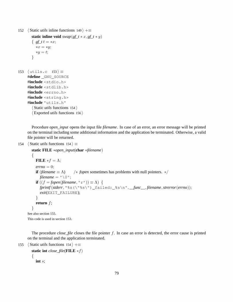
〈Staticutils inline functions149〉 +≡152
static inline void swap(gf_t ∗ x, gf_t ∗ y){ gf_t t = ∗x;∗x = ∗y;∗y = t;}
〈utils.c 153〉 ≡153#define_GNU_SOURCE#include <stdio.h>#include <stdlib.h>#include <errno.h>#include <string.h>#include "utils.h"〈Staticutils functions 154〉〈Exportedutils functions 156〉
Procedureopen_inputopens the input filefilename. In case of an error, an error message will be printedon the terminal including some additional information and the application be terminated. Otherwise, a validfile pointer will be returned.
〈Staticutils functions 154〉 ≡154
static FILE ∗open_input(char ∗filename){
FILE ∗f = Λ;
errno = 0;if (filename≡ Λ) /∗ fopensometimes has problems with null pointers.∗/
filename= "\0";if ((f = fopen(filename,"r")) ≡ Λ) {
fprintf (stderr,"%s(\"%s\") failed: %s\n", __func__, filename, strerror(errno));exit(EXIT_FAILURE);}return f ;}
See also section 155.
This code is used in section 153.
The procedureclose_filecloses the file pointerf . In case an error is detected, the error cause is printedon the terminal and the application terminated.
〈Staticutils functions 154〉 +≡155
static int close_file(FILE ∗f){
int s;
79

if (f ≡ Λ) return 0;errno = 0;s = fclose(f); /∗ fclose returns EOF if an error is detected,∗/if (s ≡ EOF) { /∗ otherwise it returns zero.∗/
fprintf (stderr,"%s failed: %s\n", __func__, strerror(errno));exit(EXIT_FAILURE);}return s;}
The procedureread_input reads the input file of the application. Entries in the input file consist ofkey=value pairs, one per line. Comments start with’#’. Empty lines are allowed. After closing theinput file, a check of the read parameters will be done. In case the parameters are not in valid ranges, theapplication will be terminated.
〈Exportedutils functions 156〉 ≡156
int read_input(char ∗fname, int ∗m, int ∗n, int ∗t, int ∗debug){
FILE ∗input = open_input(fname); /∗ open input file∗/〈Read input file157〉close_file(input); /∗ close input file∗/return 1;}
See also sections 163, 164, and 165.
This code is used in section 153.
〈Read input file157〉 ≡157char ∗ line = malloc(MAX_LINE);while ( fgets( line , MAX_LINE, input ) ) {〈Skip C comments158〉〈Terminate each line with’#’ 159〉〈Fetch the contents of the current line before the first’#’ 160〉〈Split the line at’=’ and search forkey= valuepairs 161〉}free ( line ) ;
This code is used in section 156.
CWEB produces section numbers with the following format /*<number>:*/.
〈Skip C comments158〉 ≡158if ( line [0] ≡ ’/’ ∧ line [1] ≡ ’*’ ) continue;
This code is used in section 157.
80

〈Terminate each line with’#’ 159〉 ≡159size t const len= strnlen( line , MAX_LINE ) ;line [len− 1] = ’#’;
This code is used in section 157.
〈Fetch the contents of the current line before the first’#’ 160〉 ≡160char ∗data= strchr ( line , ’#’ ) ;∗data= ’\0’;
This code is used in section 157.
〈Split the line at’=’ and search forkey= valuepairs 161〉 ≡161char ∗sp= strchr ( line , ’=’ ) ;if (sp) {∗sp= ’\0’;char ∗key= line ;
char ∗val = sp+ 1;
〈Search forkey− valuepairs. Initialize parameters.162〉}This code is used in section 157.
〈Search forkey− valuepairs. Initialize parameters.162〉 ≡162if (strstr(key,"extension-degree-m"))∗m = (unsigned int) strtol(val, (char ∗∗) Λ, 10);
else if (strstr(key,"code-length-n"))∗n = (unsigned int) strtol(val, (char ∗∗) Λ, 10);
else if (strstr(key,"correctable-errors-t"))∗t = (unsigned int) strtol(val, (char ∗∗) Λ, 10);
else if (strstr(key,"debug"))∗debug= (unsigned int) strtol(val, (char ∗∗) Λ, 10);
This code is used in section 161.
〈Exportedutils functions 156〉 +≡163
void print_matrix(int m, int n, constgf_t∗mat, const char∗name){
printf ("\n%s\n", name); /∗ print mat ∈ Fm×nq ∗/
for (int i = 0; i < m; ++i) {if (i %m ≡ 0) printf ("\n");for (int j = 0; j < n; ++j) {
if (j %m ≡ 0) printf ("+ ");printf ("%04x ",mat[i ∗ n+ j]);}printf ("\n");}}
81

〈Exportedutils functions 156〉 +≡164
void print_bin_matrix(int m, int n, const binmat t mat, const char∗name){
printf ("\n%s\n", name); /∗ print mat ∈ Fm×n2 ∗/
for (int i = 0; i < m; ++i) {if (i %m ≡ 0) printf ("\n");for (int j = 0; j < n; ++j) {
if (j %m ≡ 0) printf ("+ ");printf ("%ld ",mat_coeff(mat, i, j));}printf ("\n");}}
e_old is an array of lengthn, staring witht 1’s, followed byn− t 0’s:
eold = [1, 1, . . . , 1︸ ︷︷ ︸
t
, 0, 0, . . . , 0︸ ︷︷ ︸
n−t
].
Each new error vectore_newis just a random permutation ofe_old. To perform this random permutation,next_error_vectoris an implementation of AlgorithmP (see [16], p. 145) in itsinside−out version [10, 13].
〈Exportedutils functions 156〉 +≡165
void next_error_vector(const int ∗e_old, int ∗e_new, int ∗src, int ∗r, int ∗p, int n) { static int init = 0;int i;
if (init ≡ 0) {init = 1;for (i = 0; i < n; ++i) src[i] = i;srand((unsigned) rdtsc( ));r[0] = 0;for (i = 1; i < n; ++i) r[i] = rand( ) % (i+ 1);}〈Shuffle permutation166〉for (i = 0; i < n; ++i) /∗ Update error vector∗/
e_new[i] = e_old[p[i]];}
〈Shuffle permutation166〉 ≡166
p[0] = src[0];for (i = 1; i < n; ++i) {
register int j = r[i− 1];
p[i] = p[j];p[j] = src[i];}
82

for (i = 0; i < n; ++i) /∗ Update source vector for next round∗/src[i] = p[i];
This code is used in section 165.
10.3.1 Input file
The input file containskey− valuepairs. It is written byCWEB, resp.cweave.
〈input.txt 168〉 ≡168extension− degree−m = 6code− length− n = 32correctable− errors− t = 4debug= 0
11 Putting everything together
11.1 The main program
#define_GNU_SOURCE170
#include <stdio.h>#include <stdlib.h>#include <inttypes.h>#include <math.h>#include <string.h>#include "gf.h"#include "matrix.h"#include "poly.h"#include "utils.h"#include "alternant-decode.h"#include "fwht.h"#include "dyadic-convolution.h"#include "binary-quasi-dyadic-goppa-code.h"
int main(int argc, char ∗∗argv){
83

〈maindefine variables171〉〈main read the application parameters172〉〈main initialize data173〉〈maingenerate binary Goppa code of type[n, k, t] 174〉〈mainperform the encode/decode cycle175〉〈main free resources190〉return (EXIT_SUCCESS);
}
〈maindefine variables171〉 ≡171int m, q; /∗extension degree,q = 2m ∗/int n; /∗ code length∗/int N ; /∗ code length, for future use∗/int t; /∗number of correctable errors∗/int debug= 0; /∗debug flag∗/int ∗b = Λ; /∗auxiliary array, seebinary_quasi_dyadic_goppa_code∗/gf_t ∗ h = Λ; /∗auxiliary array, seebinary_quasi_dyadic_goppa_code∗/gf_t omega; /∗auxiliary variable, seebinary_quasi_dyadic_goppa_code∗/int C; /∗auxiliary variable, seebinary_quasi_dyadic_goppa_code∗/int bc; /∗auxiliary variable for block count, seebinary_quasi_dyadic_goppa_code∗/gf_t ∗H = Λ; /∗auxiliary parity check matrix. used to buildG ∗/gf_t ∗ H2T = Λ; /∗private parity check matrixH ∈ F
2t×n2m ∗/
gf_t ∗ z = Λ; /∗ root set for the Goppa polynomial∗/gf_t ∗ L = Λ; /∗ support of the binary Goppa code∗/binmat t Hbin = Λ; /∗auxiliary binary parity check matrixH ∈ F
mt×n2 in sys. from∗/
binmat t Gbin = Λ; /∗binary generator matrixG ∈ F(n−mt)×n2 ∗/
poly t poly_sigma= Λ; /∗error locator polynomialσ(X) ∈ F2m [X] ∗/poly t poly_omega= Λ; /∗error evaluator polynomialω(X) ∈ F2m [X] ∗/poly t g = Λ; /∗ the Goppa polynomialg(X) ∈ F2m [X] ∗/poly t g2 = Λ; /∗ square of the Goppa polynomialg(X)2 ∈ F2m [X] ∗/poly t SyM= Λ; /∗ the syndrome polynomialS(X) ∈ F2m [X] ∗/gf_t ∗ cw = Λ;gf_t ∗ dyadic_cw= Λ;gf_t ∗ direct_cw= Λ; /∗auxiliary arrays for testing the encode/decode cycle∗/int ∗msg= Λ; /∗auxiliary message array for testing the encode/decode cycle∗/int ∗e_old= Λ;int ∗e_new= Λ;int ∗src = Λ;int ∗rndm= Λ;int ∗perm= Λ; /∗auxiliary arrays for generating the error vector∗/
This code is used in section 170.
〈main read the application parameters172〉 ≡172
84

if (argc 6= 2) {fprintf (stderr,"usage: %s <cmd-file>\n", argv[0]);exit(−1);}if (read_input(argv[1],&m,&n,&t,&debug)) {
if (debug≥ 1) {printf ("extension-degree-m ..... %5d\n",m);printf ("code-length-n .......... %5d\n", n);printf ("correctable-errors-t ... %5d\n", t);printf ("debug .................. %5d\n", debug);}}
This code is used in section 170.
For demonstration purposes fix the values form, t andn.
〈main initialize data173〉 ≡173#defineDEGREE 6#defineCL 32#defineTN 4N = CL;n = CL;t = TN;m = DEGREE;q = 1≪ DEGREE;C = (int ) floor(q/t);cw = calloc(n, sizeof(∗cw));dyadic_cw= calloc(n, sizeof(∗dyadic_cw));direct_cw= calloc(n, sizeof(∗direct_cw));msg= calloc(n−m ∗ t, sizeof(∗msg));e_old= calloc(n, sizeof(∗e_old));e_new= calloc(n, sizeof(∗e_new));src = calloc(n, sizeof(∗src));rndm= calloc(n, sizeof(∗rndm));perm= calloc(n, sizeof(∗perm));H = calloc(t ∗ n, sizeof(∗H));h = calloc(q, sizeof(∗h));b = calloc(C, sizeof(∗b));z = calloc(t, sizeof(∗z));L = calloc(N, sizeof(∗L));gf_init(m); /∗ initialize the underlying finite fieldF2m ∗/
This code is used in section 170.
Run Algorithm2 from [4] to getz andL, then assemble the Goppa polynomialg(X) and buildH2T ,which will be used in the private decoder.
85

〈maingenerate binary Goppa code of type[n, k, t] 174〉 ≡174〈mainbuild quasi-dyadic Goppa code76〉〈mainassemble the Goppa polynomial82〉〈mainconstruct parity check matrixH2T for the private decoder115〉
This code is used in section 170.
For the chosen parameters(m = 6, t = 4, n = 32) there are28 = 256 possible messagesm. Encode anddecode all of them for a randomly generated binary Goppa code. The codewordsmG have errors ont = 4positions.
〈mainperform the encode/decode cycle175〉 ≡175〈maingenerate codewords183〉〈maindecode forged codewords185〉return 0;
This code is used in section 170.
Reverse the bits inline. This is due to the data layout ofHyMES. Additionally, little endian format isassumed.
〈main reverse signature bits ofline 176〉 ≡176line . l = rev ( line . l ) ;
This code is used in sections 177 and 178.
For some values oft and depending on the available hardware, it might be more convenient to computethe productmG directly using one of thevm-functions.
[
1 0 0 1 1 0 1 1]
︸ ︷︷ ︸
m
·
1 0 0 0 0 0 0 0 1 1 0 1 1 1 1 1 0 0 1 0 1 0 0 1 1 0 1 0 0 1 0 10 1 0 0 0 0 0 0 1 1 1 0 1 1 1 1 0 0 0 1 0 1 1 0 0 1 0 1 1 0 1 00 0 1 0 0 0 0 0 0 1 1 1 1 1 1 1 1 0 0 0 0 1 1 0 1 0 1 0 0 1 0 10 0 0 1 0 0 0 0 1 0 1 1 1 1 1 1 0 1 0 0 1 0 0 1 0 1 0 1 1 0 1 00 0 0 0 1 0 0 0 0 0 0 1 0 1 1 0 1 0 1 1 1 0 0 0 0 1 1 0 1 1 1 00 0 0 0 0 1 0 0 0 0 1 0 1 0 0 1 0 1 1 1 0 1 0 0 1 0 0 1 1 1 0 10 0 0 0 0 0 1 0 0 1 0 0 1 0 0 1 1 1 1 0 0 0 1 0 1 0 0 1 1 0 1 10 0 0 0 0 0 0 1 1 0 0 0 0 1 1 0 1 1 0 1 0 0 0 1 0 1 1 0 0 1 1 1
︸ ︷︷ ︸
G
(11.1.1)
For the productmG only the parts of the two lines ofG indicated by the boxes are necessary. There are2msuch boxes for these two lines, wherem denotes the extension degree. Due to the data layout ofHyMES,the bits of the lines have to be reversed, however. The messagem is also seen as two blocks of4 bits. Usingvm4(because oft = 4) allows now to performmG directly without the need to unfoldG first.
〈maincompute codeword directly usingvm4 177〉 ≡177
union {unsigned int l;unsigned charc[4];} line ;
86

unsigned charmesg;unsigned int codeword= k ≪ 24;for (int j = 0; j < 2; ++j){ line . l = (unsigned int)(Gbin~ elem[j ∗ t]);〈main reverse signature bits ofline 176〉mesg= ((unsigned char)(k)≫ ((j & 1) ? 0 : 4)) & #0F; /∗ pick 4 bits of mesg∗/for (int i = 1; i ≤ m; ++i) /∗ loop over the blocks of the line∗/{ codeword⊕= vm4(mesg, line . c[(m− i)/2]≫ ((i& 1) ? 4 : 0) & #0F )≪ (24− i ∗ 4); }}for (int i = 0; i < 32; ++i) /∗ savecodewordfor following equality check∗/
direct_cw[i] = (codeword≫ (31− i)) & 1;This code is used in section 183.
The productmG can also be computed using the Walsh-Hadamard transform. As with the directmethod(see (11.1.1)), only two lines ofG are necessary. However, because we have characteristic2, the transformcan not be directly applied, but has to be lifted toZ. This costs some extra memory.
〈maincompute codeword usingWalsh− Hadamard transformanddyadic convolution178〉 ≡178
for (int i = 0; i < n; ++i) /∗ first 8 bist of the codeword are known∗/dyadic_cw[i] = (i < 8) ? ((k ≫ (7− i)) & 1) : 0;
for (int j = 0; j < 2; ++j) {line . l = (unsigned int)(Gbin~ elem[j ∗ t]);〈main reverse signature bits ofline 176〉mesg= ((unsigned char)(k)≫ ((j & 1) ? 0 : 4)) & #0F;〈mainhandle blocks via Walsh-Hadamard transform179〉}for (int i = 0; i < n; ++i) /∗ reduce the result fromZ to F2 ∗/
dyadic_cw[i] &= 1;This code is used in section 183.
The vectorsu andv receive4 bits of the message and one block of the current line, respectively. ThentheWalsh− Hadamardtransformis applied to deliver the vectorw such that∆(w) = ∆(u)∆(v).
〈mainhandle blocks via Walsh-Hadamard transform179〉 ≡179fwht t u[4], v[4], ∗w;unsigned charmtrx;for (int i = 1; i ≤ m; ++i) { /∗ loop over the blocks of the line∗/mtrx= line . c[(m− i)/2]≫ ((i& 1) ? 4 : 0) & #0F;for (int ix = 0; ix < 4; ++ix) { u[3− ix] = (mesg≫ ix) & 1; v[3− ix] = (mtrx≫ ix) & 1; }〈maincompute dyadic convolution via Walsh-Hadamard transform180〉for (int ix = 0; ix < 4; ++ix) dyadic_cw[4 + i ∗ 4 + ix] += w[ix]; }
This code is used in section 178.
Input: k ∈ N,u,v ∈ Fr with r = 2k andchar(F) 6= 2.
Output:w = u △ v ∈ Fr such that∆(u)∆(v) = ∆(u △ v).
87

〈maincompute dyadic convolution via Walsh-Hadamard transform180〉 ≡180
w = dyadic_conv(2, u, v);This code is used in section 179.
Perform the productbG using the unfoldedG.
〈maincompute codeword explicitly as vector-matrix product181〉 ≡181for (int i = 0; i < 8; ++i)
msg[7− i] = ((1≪ i) & k)≫ i;for (int i = 0; i < n; ++i)
cw[i] = 0;for (int i = 0; i < n−m ∗ t; ++i)
if (msg[i])for (int j = 0; j < n; ++j)
cw[j] = (cw[j] + mat_coeff(Gbin, i, j)) & 1;This code is used in sections 183 and 185.
〈maincheck equality of codewords182〉 ≡182
for (int i = 0; i < n; ++i)if ((direct_cw[i] 6= dyadic_cw[i]) ∨ (direct_cw[i] 6= cw[i]))
fprintf (stderr,"ERROR in cw. comp.: %d %X,%X,%X", i, direct_cw[i], dyadic_cw[i],cw[i]);
This code is used in section 183.
For demonstration purposes, the three different methods of performingmG are shown.
〈maingenerate codewords183〉 ≡183if (t ≡ 4 ∧ n ≡ 32 ∧m ≡ 6) {〈Print generator matrix G93〉
for (int k = 0; k < 256; ++k) {〈maincompute codeword directly usingvm4 177〉〈maincompute codeword explicitly as vector-matrix product181〉〈maincompute codeword usingWalsh− Hadamard transformanddyadic convolution178〉〈maincheck equality of codewords182〉}}
This code is used in section 175.
〈maingenerate next error vector184〉 ≡184next_error_vector(e_old, e_new, src, rndm, perm, n);
This code is used in section 185.
88
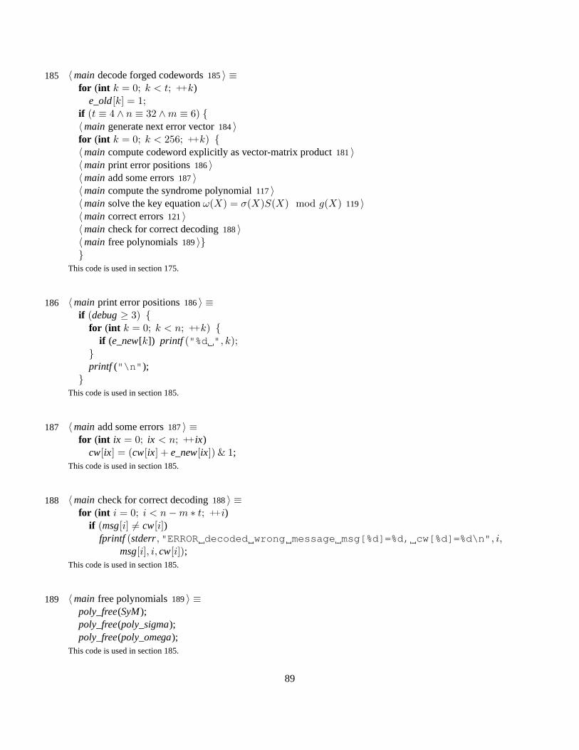
〈maindecode forged codewords185〉 ≡185for (int k = 0; k < t; ++k)
e_old[k] = 1;if (t ≡ 4 ∧ n ≡ 32 ∧m ≡ 6) {〈maingenerate next error vector184〉for (int k = 0; k < 256; ++k) {〈maincompute codeword explicitly as vector-matrix product181〉〈mainprint error positions186〉〈mainadd some errors187〉〈maincompute the syndrome polynomial117〉〈mainsolve the key equationω(X) = σ(X)S(X) mod g(X) 119〉〈maincorrect errors121〉〈maincheck for correct decoding188〉〈main free polynomials189〉}}
This code is used in section 175.
〈mainprint error positions186〉 ≡186if (debug≥ 3) {
for (int k = 0; k < n; ++k) {if (e_new[k]) printf ("%d ", k);
}printf ("\n");}
This code is used in section 185.
〈mainadd some errors187〉 ≡187for (int ix = 0; ix < n; ++ix)
cw[ix] = (cw[ix] + e_new[ix]) & 1;This code is used in section 185.
〈maincheck for correct decoding188〉 ≡188for (int i = 0; i < n−m ∗ t; ++i)
if (msg[i] 6= cw[i])fprintf (stderr,"ERROR decoded wrong message msg[%d]=%d, cw[%d]=%d\n", i,
msg[i], i, cw[i]);This code is used in section 185.
〈main free polynomials189〉 ≡189poly_free(SyM);poly_free(poly_sigma);poly_free(poly_omega);
This code is used in section 185.
89

〈main free resources190〉 ≡190if (e_old 6= Λ) free(e_old);if (e_new6= Λ) free(e_new);if (src 6= Λ) free(src);if (rndm 6= Λ) free(rndm);if (perm 6= Λ) free(perm);if (cw 6= Λ) free(cw);if (dyadic_cw6= Λ) free(dyadic_cw);if (direct_cw 6= Λ) free(direct_cw);if (msg 6= Λ) free(msg);if (Hbin 6= Λ) mat_free(Hbin);if (Gbin 6= Λ) mat_free(Gbin);if (z 6= Λ) free(z);if (L 6= Λ) free(L);if (b 6= Λ) free(b);if (h 6= Λ) free(h);if (H 6= Λ) free(H);if (H2T 6= Λ) free(H2T);gf_free( );
This code is used in section 170.
12 Known issues and further improvements
In order to hide the dyadic code structure, there are some measures takenin [23]. To be compliant, theGoppa code generated bybinary_quasi_dyadic_goppa_codeshould have code lengthN , whereN ≫ n.To arrive at a code with lengthn, blocks would have to be selected, rearranged and permuted using dyadicpermutations. However, we skip this step and rely completely on the secret and permuted supportL. Asalready mentioned, one of the reasons for this practice is simplicity. Another factor was the structural attackagainst the scheme (see part (VI)). The attack was successful in non-binary cases, so it is not clear if thosecode hiding techniques could be more effective in the binary case.
Furthermore, the algorithm implemented inbinary_quasi_dyadic_goppa_codespuriously yields an er-roneous supportL, in which case the code generation is restarted. It is at the moment not clearif this is abug in the code or a design error of the algorithm itself.
90

Part VIII
Appendix
13 Basic algebraic structures
Coding theory is concerned with the transmission ofmessagesover an unreliable channel. Transmissionerrors can occur and the question arises how to possibly recognize or even correct them.
The messages to be sent are seen as fixed-length sequences of symbolsover a fixed alphabet. As wewill work with so-calledlinear (block) codes, the messages will be seen as elements of a k-dimensionalsubvector space over the finite fieldFn
q .27 Thus, eachencodedmessage will consist of a fixed number ofsymbols ofFn
q .The algebraic structure of linear codes is utilized for efficientencodinganddecodingtechniques. Alge-
bra is therefore the most important tool when dealing with linear codes.For convenience, we will recall some definitions and facts in the Appendix,which will be used below.
Details can be found for example in [27, 28, 34, 33].
13.1 Monoid, group and field
Definition 13.1.1(Semigroup, monoid, group).
(i) A set(M, ∗) together with an associative operation∗ is called asemigroup.
(ii) If the operation does have a neutral elemente, then(M, ∗) is called amonoid.
(iii) A subsetM ′ ⊆M , e ∈M ′, which is closed under the monoid operation is calledsubmonoidofM .
(iv) A group28 is a monoid in(M, ∗) in which every elementa ∈ M is invertible, i.e. for all a ∈ Mthere exists ana′ ∈ M such thata ∗ a′ = a′ ∗ a = e. Additionally, it holds for alla ∈ M thata ∗ e = e ∗ a = a.
(v) A groupM, ∗ such that for alla, a′ ∈M it holds thata∗a′ = a′ ∗a is called acommutativeor abeliangroup. It is usually denoted by(M,+).
Definition 13.1.2(Ring). Let (A,+, ·) be a set together with two operations calledadditionand multipli-cation. A is called a ring with respect to these operations if the following conditions hold:
(i) (A,+) is an abelian group, called theadditive groupofA.
27Frequently the scalar ring denoted also asGF (q), theGalois fieldwith q elements, named afterEvariste Galois.28The namegroupgoes back again to Galois [28].
91

(ii) (A, ·) is a monoid, called themultiplicative monoidofA.29
(iii) For all a, b, c ∈ A hold
1. a(b + c) = ab + ac
2. (b + c)a = ba + ca
(iv) The ring A is calledcommutativeif (A, ·) is abelian.
Definition 13.1.3(Subring, ring extension). LetA be a ring. A subsetU ⊆ A is called asubringof A if(U,+, ·) is itself a ring. We writeS ≤ A to express thatU is a subring ofA and also call[A : U ] a ringextension. If 1A ∈ U then we call[A : U ] a unital ring extension.
Definition 13.1.4(Characteristic). LetA be a ring. Thecharacteristic charA of A is the smallest numbern ∈ N such thatn · 1 = 0. If no suchn exists, we say thatcharA = 0.
Definition 13.1.5(Units, unital group). Let A be a ring.Invertible elementsa ∈ (A, ·) are calledunits. They form theunital groupof A, denoted byA×.
Definition 13.1.6(Zero-divisor). LetA be a ring.An elementa 6= 0 in A is called azero-divisorif there is an elements 6= 0 such thatrs = 0 or sr = 0.
Definition 13.1.7(Integral domain, field, subfield). LetA be a commutative ring.
(i) A is anintegral domainif it has no zero-divisors.
(ii) An integral domain is called afield if a|b for any two elementsa ∈ Ar {0} andb ∈ A.
(iii) Is a subringU of a ringA a field, we say thatU is asubfieldofA.
Remark 13.1.8. We will deal only with so-calledfinite fields, i.e. fields with a finite number ofq elements(q ∈ N). It will be denoted byFq. The number of elements ofFq is called itsorder. As can be shown [27],the characteristic of a finite field is always a prime numberp.
13.2 Direct product and direct sum
Definition 13.2.1(Direct product). Let I 6= ∅ a non-empty index set and letMi, i ∈ I a system of sets withMi 6= ∅ for all i ∈ I. LetM :=
⋃
i∈I Mi. The set of families{f : I →M | fi := f(i) ∈Mi for all i ∈ I
}
is called thedirector cartesian productof theMi.30 It is denoted by∏
i∈I Mi.If theMi are monoids for alli ∈ I, thenM is a monoid relative the following operation:M×M →M ,
((ai)i∈I , (bi)i∈I) 7→ ((aibi)i∈I). It is called theproduct monoidof theMi.If all Mi = M for a setM , then
∏
i∈I Mi = M I ={f | f : I →M
}, the set of all mappings fromI to
M . It is called theI-fold productofM .
29Hence rings as defined here will always have a multiplicative neutral elemente, denoted as1.30A common notation for such a familyf is (fi)i∈I
92

Definition 13.2.2 (Direct sum). Let I an arbitrary set,Mi monoids for alli ∈ I, and letei denote theneutral element ofMi for all i ∈ I.
∏′i∈I Mi :=
{(ai)i∈I ∈
∏
i∈I Mi | ai 6= ei for finitely manyi ∈ I}
is a submodule of∏
i∈I Mi. Is is called thedirect sumof the monoidsMi and denoted by⊕
i∈I Mi or∐
i∈I Mi.31
Remark 13.2.3.LetM a monoid,I an arbitrary set. Then∏
i∈I M is denoted byM (I) and called theI-folddirect productof the monoidsM . It is a submonoid ofM I , the direct product of the monoidsM . In caseI =
{1, . . . , n
}, thenM I = M (I) = Mn.
13.3 Module and vector space
Definition 13.3.1(Module, vector space). Let A be a ring. An abelian group V together with a (mulipica-tively denoted) operation32 of A on V is called an A-moduleif for all a, b ∈ A andx, y ∈ V hold:
(i) 1A · x = x.
(ii) a(bx) = (ab)x.
(iii) a(x+ y) = ax+ ay.
(iv) (a+ b)x = ax+ bx.
If the underlyingscalarring A is a field, then V is called avector space.
Remark 13.3.2(Direct product and direct sum of modules). Let (Vi)i∈I a family of A-modules. The directproduct
∏
i∈I Vi and the direct sum⊕
i∈I Vi =∐
i∈I Vi are A-modules bya(xi)i∈I := (axi)i∈I for a ∈ Aand (xi)i∈I . The addition in
∏
i∈I Vi resp.⊕
i∈I Vi is defined as(xi)i∈I + (yi)i∈I := (xi + yi)i∈I . If allVi = V for an A-moduleV , then
∏
i∈I = V I and⊕
i∈I Vi = V (I). If I ={1, . . . , n
}, thenV I = V (I) =
V n.
Remark 13.3.3(n-dimensional vector space). Let F a field,n ∈ N. Fn is then canonically anF-module,
i.e. an n-dimensionalF-vector space. Forx, y ∈ Fn andα ∈ F we have
x+ y := (x0, . . . , xn−1) + (y0, . . . , yn−1) := (x0 + y0, . . . , xn−1 + yn−1)αx := α(x0, . . . , xn−1) := (αx0, . . . , αxn−1)
31If I is finite, then clearly∏
i∈I Mi =∐
i∈I Mi.32An operationof a setM on a setX is a mapM ×X → X.
93
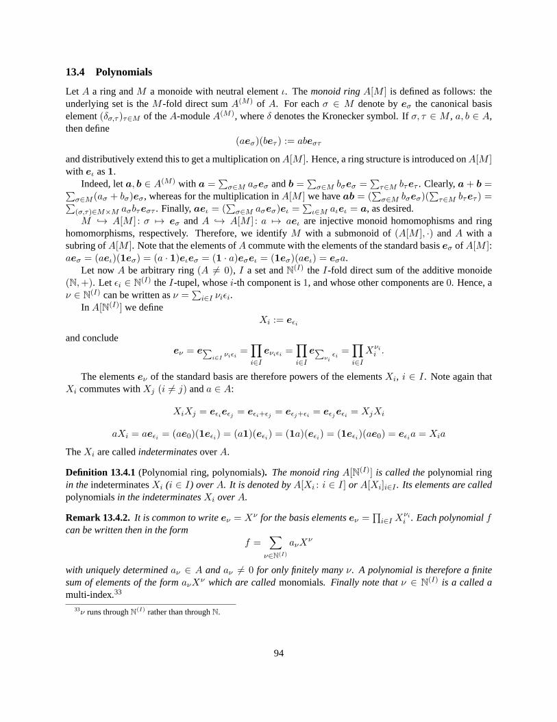
13.4 Polynomials
Let A a ring andM a monoide with neutral elementι. Themonoid ringA[M ] is defined as follows: theunderlying set is theM -fold direct sumA(M) of A. For eachσ ∈ M denote byeσ the canonical basiselement(δσ,τ )τ∈M of theA-moduleA(M), whereδ denotes the Kronecker symbol. Ifσ, τ ∈ M , a, b ∈ A,then define
(aeσ)(beτ ) := abeστ
and distributively extend this to get a multiplication onA[M ]. Hence, a ring structure is introduced onA[M ]with eι as1.
Indeed, leta, b ∈ A(M) with a =∑
σ∈M aσeσ andb =∑
σ∈M bσeσ =∑
τ∈M bτeτ . Clearly,a+ b =∑
σ∈M (aσ + bσ)eσ, whereas for the multiplication inA[M ] we haveab = (∑
σ∈M bσeσ)(∑
τ∈M bτeτ ) =∑
(σ,τ)∈M×M aσbτeστ . Finally,aeι = (∑
σ∈M aσeσ)eι =∑
ι∈M aιeι = a, as desired.M → A[M ] : σ 7→ eσ andA → A[M ] : a 7→ aeι are injective monoid homomophisms and ring
homomorphisms, respectively. Therefore, we identifyM with a submonoid of(A[M ], ·) andA with asubring ofA[M ]. Note that the elements ofA commute with the elements of the standard basiseσ of A[M ]:aeσ = (aeι)(1eσ) = (a · 1)eιeσ = (1 · a)eσeι = (1eσ)(aeι) = eσa.
Let nowA be arbitrary ring(A 6= 0), I a set andN(I) the I-fold direct sum of the additive monoide(N,+). Let ǫi ∈ N
(I) theI-tupel, whosei-th component is1, and whose other components are0. Hence, aν ∈ N
(I) can be written asν =∑
i∈I νiǫi.In A[N(I)] we define
Xi := eǫi
and concludeeν = e∑
i∈Iνiǫi
=∏
i∈I
eνiǫi =∏
i∈I
e∑νi
ǫi=
∏
i∈I
Xνii .
The elementseν of the standard basis are therefore powers of the elementsXi, i ∈ I. Note again thatXi commutes withXj (i 6= j) anda ∈ A:
XiXj = eǫieǫj = eǫi+ǫj = eǫj+ǫi = eǫjeǫi = XjXi
aXi = aeǫi = (ae0)(1eǫi) = (a1)(eǫi) = (1a)(eǫi) = (1eǫi)(ae0) = eǫia = Xia
TheXi are calledindeterminatesoverA.
Definition 13.4.1(Polynomial ring, polynomials). The monoid ringA[N(I)] is called thepolynomial ringin the indeterminatesXi (i ∈ I) overA. It is denoted byA[Xi : i ∈ I] or A[Xi]i∈I . Its elements are calledpolynomialsin the indeterminatesXi overA.
Remark 13.4.2. It is common to writeeν = Xν for the basis elementseν =∏
i∈I Xνii . Each polynomialf
can be written then in the formf =
∑
ν∈N(I)
aνXν
with uniquely determinedaν ∈ A andaν 6= 0 for only finitely manyν. A polynomial is therefore a finitesum of elements of the formaνXν which are calledmonomials. Finally note thatν ∈ N
(I) is a called amulti-index.33
33ν runs throughN(I) rather than throughN.
94

If g =∑
ν∈N(I) bνXν is another polynomial inA[N(I)], we have
f + g =∑
ν∈N(I)
(aν + bν)Xν
fg =∑
λ∈N(I)
cλXλ
with cλ :=∑
ν+µ aνbµ, whereλ, µ, ν run throughN(I).
Remark 13.4.3. Let I a set with one element. In the above construction, one has then only one indetermi-nate, denoted just byX, and we have:
f =∑
ν≥0
aνXν = a0 + a1X
1 + · · ·+ anXn,
g =∑
µ≥0
bνXν = b0 + b1X
1 + · · ·+ bmXm,
fg =∑
λ≥0
cλXλ with cλ =
λ∑
j=0
ajbλ−j = a0bλ + · · ·+ aλb0,
if aν = bµ = 0 for ν > n, µ > m.
95

References
[1] M. Braun et. al. A. Betten.Error-Correcting Linear Codes, volume 18 ofAlgorithms and Computationin Mathematics. Springer, 2006.
[2] P. S. L. M. Barreto. Post Quantum Cryptography.http://www.larc.usp.br/~pbarreto/PQC-4.pd.
[3] P. S. L. M. Barreto. The Fast Walsh-Hadamard Transform. Private communication, 2010.
[4] P. S. L. M. Barreto, P.-L. Cayrel, R. Misoczki, and R. Niebuhr. Quasi-dyadic CFS signatures. InInscrypt 2010, LNCS. Springer, 2010.
[5] P. S. L. M. Barreto, R. Lindner, and R. Misoczki. Decoding square-free Goppa codes overFp. 2010.
[6] E. Berlekamp, R. McEliece, and H. van Tilborg. On the inherent intractability of certain codingproblems.IEEE Transactions on Information Theory, 24(3):384–386, 1978.
[7] E. R. Berlekamp. Factoring polynomials over large finite fields.Mathematics of Computation,24(111):713–715, 1970.
[8] D. J. Bernstein. List decoding for binary Goppa codes, 2008.http://cr.yp.to/codes/goppalist-20110223.pdf.
[9] R. T. Chien. Cyclic decoding procedure for the bose-chaudhuri-hocquenghem codes.IEEE Transac-tions on Information Theory, 10(4):357–363, 1964.
[10] R. Durstenfeld. Algorithm 235: Random Permutation.Communications of the ACM, 7(7):420, 1964.
[11] D. Engelbert, R. Overbeck, and A. Schmidt. A summary of McEliece-type cryptosystems and theirsecurity.Journal of Mathematical Cryptology, 1:151–199, 2007.
[12] J.-C. Faugère, A. Otmani, L. Perret, and J.-P. Tillich. Algebraic cryptanalysis of McEliece variantswith compact keys. InAdvances in Cryptology – Eurocrypt’2010, LNCS. Springer, 2010.
[13] R. A. Fisher and F. Yates. Statistical tables for biological, agricultural and medical research, 1948,(1938).http://en.wikipedia.org/wiki/Fisher-Yates_shuffle.
[14] B. Friedrichs. Kanalcodierung, Grundlagen und Anwendungen in modernen Kommunikationssyste-men. Springer, 1996.
[15] A. Joux. Algorithmic Cryptanalysis. Cryptography and Network Security. Chapman and Hall/CRC,2009.
[16] D. E. Knuth. The Art of Computer Programming, 2. Seminumerical Algorithms. Addison-Wesley,2005.
[17] D. E. Knuth and S. Levy.The CWEB System of Structured Documentation. Addison-Wesley Profes-sional, 1994.http://www-cs-faculty.stanford.edu/~uno/cweb.html.
96
[18] E. Kunz.Algebra. Vieweg, 1991.
[19] R. Lidl and H. Niederreiter.Finite Fields. Number 20 in Encyclopedia of Mathematics and its Appli-cations. Cambridge University Press, Cambridge, UK, 2nd edition, 1997.
[20] F. J. MacWilliams and N. J. A. Sloane.The theory of error-correcting codes, volume 16. North-HollandMathematical Library, 1977.
[21] R. McEliece. A public-key cryptosystem based on algebraic codingtheory. The DeepSpace Network Progress Report, DSN PR 42–44, 1978.http://ipnpr.jpl.nasa.gov/progressreport2/42-44/44N.PDF.
[22] R. J. McEliece.The Theory of Information and Coding. Encyclopedia of Mathematics and its Appli-cations. Addison-Wesley, 1978.
[23] R. Misoczki and P. S. L. M. Barreto. Compact McEliece keys fromGoppa codes. InSelected Areas inCryptography – SAC’2009, volume 5867 ofLNCS, pages 276–392. Springer, 2009.
[24] N. J. Patterson. The algebraic decoding of Goppa codes.IEEE Transactions on Information Theory,21(2):203–207, 1975.
[25] E. Persichetti. Compact McEliece keys based on Quasi-Dyadic Srivastava codes, 2011.http://eprint.iacr.org/2011/179.pdf.
[26] S. Roman.Coding and Information Theory, Graduate Texts in Mathematics. Springer, 1992.
[27] G. Scheja and U. Storch.Lehrbuch der Algebra, volume 1. Teubner, 1980.
[28] G. Scheja and U. Storch.Lehrbuch der Algebra, volume 2. Teubner, 1988.
[29] N. Sendrier and B. Biswas. Hymes, The Hybrid McEliece Encription Scheme.http://www-rocq.inria.fr/secret/CBCrypto/index.php?pg=hymes.
[30] N. Sendrier and B. Biswas. McEliece Cryptosystem Implementation: Theory and Practice. InPost-Quantum Cryptography, volume 5299 ofLNCS, 2008.
[31] C. E. Shannon. A Mathematical Theory of Communication and Communication, Theory of SecrecySystems.Bell System Tech. J., 1948.
[32] P. W. Shor. Polynomial-Time Algorithms for Prime Factorization and Discrete Logarithms on a Quan-tum Computer.SIAM Journal on Computing, 26:1484–1509, 1995.
[33] K. Spindler.Abstract Algebra with Applications: Rings and Fields. Dekker, 1994.
[34] K. Spindler.Abstract Algebra with Applications: Vector Spaces and Groups. Dekker, 1994.
[35] H. Stichtenoth. Algebraic Function Fields and Codes. Graduate Texts in Mathematics. Springer,Berlin, Heidelberg, 2nd edition, 2009.
[36] K. K. Tzeng and K. Zimmermann. On extending Goppa codes to cyclic codes.IEEE Transactions onInformation Theory, 21:721–716, 1975.
[37] H. S. Warren.Hacker’s Delight. Addison-Wesley, 2003.
97

Index
Here is a list of the identifiers used, and where they appear. Underlined entries indicate the place of defini-tion. Error messages are also shown.
__asm__: 151.__func__: 154, 155._gf_modq_1: 39._GNU_SOURCE: 138, 153, 170.A: 137, 139, 140, 141, 142, 143, 144, 145, 146.a: 137, 143.add: 101.alloc_size: 137, 139, 140, 146.ALTERNANT_DECODE_H_INCLUDED: 110.argc: 170, 172.argv: 170, 172.assert: 143.aux: 135.a0: 83.a1: 83.B: 137, 146.b: 58, 62, 137, 143, 171.bc: 58, 62, 74, 77, 83,171.BINARY_QD_GOPPA_CODE_H_INC: 57.binary_quasi_dyadic_goppa_code: 58, 62,
77, 191.binmat t : 137, 139, 140, 141, 142, 143, 144,
145, 146, 148, 164, 171.bit: 101.BITS_PER_LONG: 85, 137, 139, 140.C: 62, 146, 171.c: 62, 177.calloc: 113, 126, 130, 173.CL: 173.close_file: 155, 156.code: 168.codeword: 177.coeff: 124, 126, 127, 128, 129, 130, 131,
133, 134.coln: 137, 139, 140, 142, 144, 146.cons_parity_check: 110, 113, 115.cons_syndrome_polynomial: 110, 116, 117.consistent_root_set: 72.consistent_support_block: 73.correctable: 168.cR: 137, 145.
cw: 110, 117, 121, 171, 173, 181, 182, 187,188, 190.
cweave: 167.CWEB: 167.d: 99, 124, 126, 128, 131, 133.data: 160.debug: 58, 62, 70, 77, 78, 83, 85, 87, 89,
92, 110, 113, 115, 148, 156, 162, 168,171, 172, 186.
deg: 124, 126, 128, 129, 130, 131.degree: 168.DEGREE: 173.delta: 135.direct_cw: 171, 173, 177, 182, 190.done_building_goppa_code: 76.dp: 132.dq: 132.dr: 135.du: 135.dyadic_conv: 106, 108, 180.DYADIC_CONVOLUTION_H_INCLUDED:
106.dyadic_cw: 171, 173, 178, 179, 182, 190.e: 89.e_new: 148, 165, 171, 173, 184, 186, 187, 190.e_old: 148, 165, 171, 173, 184, 185, 190.elem: 85, 89,137, 139, 140, 141, 142, 143,
145, 146, 177, 178.elt: 60.EOF: 155.errno: 154, 155.errors: 168.exit: 46, 63, 64, 146, 154, 155, 172.EXIT_FAILURE: 46, 154, 155.EXIT_SUCCESS: 170.extdeg: 37, 46.extension: 168.f : 154, 155.failcnt: 144.fclose: 155.fgets: 157.
98

filename: 154.findrow: 144.floor: 173.fname: 148, 156.fopen: 154.fprintf : 46, 63, 64, 70, 79, 80, 81, 85, 87, 91,
92, 154, 155, 172, 182, 188.free: 48, 74, 87, 113, 127, 141, 144, 157, 190.fwht: 95, 96, 99, 108.FWHT_H_INCLUDED: 96.fwht t : 96, 99, 106, 108, 179.g: 124, 135, 171.Gbin: 91, 92, 93,171, 177, 178, 181, 190.gf_add: 39, 70, 72, 73, 78, 83, 84, 113, 116,
124, 133.gf_card: 38, 41, 46.gf_div: 39, 135.gf_exp: 38, 39, 41, 48, 49, 50, 51, 52, 54, 61, 66.gf_extd: 38, 39,41, 46, 50, 52, 54.gf_free: 37, 46, 48, 190.GF_H_INCLUDED: 35.gf_init: 37, 45, 46, 173.gf_init_exp: 46, 50.gf_init_log: 46, 52.gf_inv: 39, 70, 72, 73, 78, 83, 84, 113.gf_log: 38, 39, 41, 48, 51, 52, 54.gf_mul: 39, 113, 116, 124, 132, 133.gf_mul_fast: 39, 135.gf_ord: 38, 39,41, 46, 50, 52, 54.gf_pow: 37, 53, 54.gf_rand: 37.gf_sqrt: 39.gf_square: 39.gf_t: 36,37, 38, 41,54, 58, 61, 62, 83,85, 110,
113, 116, 124, 126, 128, 129, 130,133, 134,135, 148, 152,163, 171.
gf_unit: 39, 135.gf_zero: 39, 131, 133, 135.g2: 82, 110, 113, 115, 118, 119,171.h: 99, 148.Hadamard: 99, 179.Hbin: 85, 86, 87, 88, 89, 90, 91, 92,171, 190.Hbin_in_systematic_form: 87, 88.HyMES: 87, 88, 176, 177.H2: 113.
H2T: 110, 113, 114, 115,116, 117, 171, 190.i: 37, 50, 52, 54, 69, 72, 73, 74, 78, 79, 80,
81, 82, 83, 84, 85, 88, 89, 91, 92, 99, 101,102, 103, 104, 113, 116, 121, 132, 135,142, 143, 144, 145, 146, 163, 164, 165, 177,178, 179, 181, 182, 188.
idx: 85, 144.in: 101.init : 165.init_done: 44, 46.INIT_U_RANDOM: 61, 71.input: 156, 157.inside: 165.inttypes: 36.ix: 179, 187.j: 70, 73, 79, 80, 81, 83, 84, 85, 88, 89, 91,
92, 99, 113, 116, 132, 135, 144, 145, 146,163, 164, 166, 177, 178, 181.
k: 62, 85, 91, 96, 99, 106, 108, 146, 183,185, 186.
key: 161, 162, 167.L: 110, 113.l: 60, 177.len: 159.length: 168.m: 96, 103, 148, 156, 163, 164, 171.main: 115, 121,170.malloc: 50, 52, 64, 126, 130, 139, 140,
144, 157.mat: 148, 163, 164.mat_change_coeff: 137, 146.mat_coeff: 88, 91, 92,137, 144, 146, 164, 181.mat_copy: 137, 142.mat_free: 85, 92,137, 141, 190.mat_ini: 85, 92,137, 139, 142, 146.mat_ini_from_string: 137, 140.mat_mul: 137, 146.mat_rowxor: 137, 143, 144.mat_rref: 87, 88,137, 144.mat_set_coeff_to_one: 92, 137.mat_set_to_zero: 85, 92,137.mat_vec_mul: 137, 145.matrix : 137, 140.MATRIX_H_INCLUDED: 137.max: 144.
99

MAX_EXT_DEG: 36, 42, 43, 46.MAX_LINE: 148, 157, 159.memcpy: 128, 130.memset: 72, 128, 129, 137, 145, 146.mesg: 177, 178, 179.msg: 171, 173, 181, 188, 190.mtrx: 179.N : 171.n: 101, 102, 103, 104, 110, 113, 116, 148,
156, 163, 164, 165, 171.name: 148, 163, 164.next_error_vector: 148, 165, 184.omega: 58, 62, 74, 77, 78, 83, 110, 171.open_input: 154, 156.out: 165.p: 99, 108, 124, 126, 127, 128, 129, 130, 131,
132, 134, 135, 165.p_old: 82.perm: 87, 88,144, 148, 171, 173, 184, 190.poly_addto_coeff: 124, 132, 135.poly_alloc: 82, 116,124, 126, 132, 135.poly_calcule_deg: 82, 116, 121,124, 128,
131, 132.poly_coeff: 113,124, 132, 135.poly_copy: 82, 124, 130.poly_deg: 124, 132, 134, 135.poly_eeaux: 118, 124, 135.poly_eval: 113, 121, 124, 134.poly_eval_aux: 133, 134.poly_free: 82, 124, 127, 135, 189.POLY_H_INCLUDED: 124.poly_mul: 82, 124, 132.poly_multo_coeff: 124.poly_omega: 118, 119, 121,171, 189.poly_set: 124, 128, 135.poly_set_coeff: 82, 116,124, 135.poly_set_deg: 124, 135.poly_set_to_zero: 124, 129, 135.poly_sigma: 118, 119, 121,171, 189.poly_size: 124.poly t : 82,110, 113,116, 118,124, 126, 127,
128, 129, 130, 131, 132, 134, 135, 171.poly_tete: 124.polynome: 124, 126, 130.pop: 150.
prim_poly: 42, 43, 50.print_bin_matrix: 86, 90, 93,148, 164.print_matrix: 114, 148, 163.printf : 78, 83, 163, 164, 172, 186.pt: 145.q: 62, 99, 108, 124, 128, 130, 132, 171.r: 99, 103, 108, 132, 165.rand: 61, 165.rdtsc: 66, 151, 165.read_input: 148, 156, 172.REMOVE_FROM_U: 60, 69, 70, 72, 73.res: 101, 102,103, 104.rev: 149, 176.rndm: 148, 171, 173, 184, 190.row: 101, 102.rown: 89, 137, 139, 140, 142, 143, 144,
145, 146.rwdcnt: 85, 89,137, 139, 140, 142, 143, 145.r0: 135.r1: 135.s: 68, 99, 137, 140, 155.set: 101.sigma: 110.size: 124, 126, 128, 129, 130, 131.solve_key_equation: 110, 118, 119.sp: 161.srand: 66, 165.src: 148, 165, 166,171, 173, 184, 190.stderr: 46, 63, 64, 70, 79, 80, 81, 85, 87, 91,
92, 154, 155, 172, 182, 188.strchr: 160, 161.strerror: 154, 155.strnlen: 159.strstr: 162.strtol: 162.swap: 152.SyM: 117, 119,171, 189.t: 110, 118, 124, 135, 148, 156, 171.tmp: 61.TN: 173.transform: 99, 179.tt: 110, 113, 114, 116.u: 61, 96, 99, 106, 108, 116, 124, 135, 179.uint16 t : 36, 96, 103.uint32_t: 58, 62,96, 104.
100

uint8_t: 96, 101, 102.UTILS_H_INCLUDED: 148.u0: 135.u1: 135.u8rnd: 37.v: 61, 96, 99, 103, 106, 108, 124, 135, 179.val: 161, 162.value: 167.vm: 95, 101, 177.vm16: 96, 103.vm2x4: 96.vm32: 96, 104.vm4: 95, 96, 102, 177.vm8: 96, 101.w: 99, 148, 179.Walsh: 99, 179.X: 142.x: 91, 137, 145, 149, 150, 151.
101

List of Refinements
〈 i← 2s, hi$←U, U ← U \ {hi} 69〉 Used in section 68.
〈 q ← 2m; exit in case code lengthn > q/2; initialize underlying field bufferU : U ← Fq \ {0} 64〉 Used
in section 62.
〈Call binary_quasi_dyadic_goppa_code77〉 Used in section 76.
〈Change row order89〉 Used in section 87.
〈CheckGHT = 0 91〉 Used in section 92.
〈CheckL for consistency80〉 Used in section 76.
〈Checkz ∩L = ∅ 81〉 Used in section 76.
〈Checkz for consistency79〉 Used in section 76.
〈Check Hbin for systematic form88〉 Used in section 87.
〈Check for consistent root and support set72〉 Used in section 65.
〈Check ift is a power of2; exit in case it is not or in caset > (2m − 1)/m 63〉 Used in section 62.
〈Computez 78〉 Used in section 76.
〈ComputeH ∈ Ft×nq 84〉 Used in section 76.
〈Compute the co-trace matrix85〉 Used in section 76.
〈Compute the support83〉 Used in section 76.
〈Definefield variables41〉 Used in section 40.
〈Determine consistent support blocks{hjt, . . . , h(j+1)t−1} 73〉 Used in section 72.
〈Determine the remaining signature entrieshn (1 ≤ n ≤ q − 1) 68〉 Used in section 65.
〈Exporteddyadicfunctions 58〉 Used in section 57.
〈Exportedfield declarations36〉 Used in section 35.
〈Exportedfield functions 37〉 Used in section 35.
〈Exportedfield macros39〉 Used in section 35.
〈Exportedfield variables38〉 Used in section 35.
〈Exportedmatrix functions 139, 140, 141, 142, 143, 144, 145, 146〉 Used in section 138.
〈Exportedpoly functions 126, 127, 128, 129, 130, 131, 132, 134, 135〉 Used in section 125.
〈Exportedutils functions 156, 163, 164, 165〉 Used in section 153.
〈Fetch the contents of the current line before the first’#’ 160〉 Used in section 157.
〈Generate consistent root and support sets.65〉 Used in section 62.
〈Generate nexthi+j for 1 ≤ j ≤ i− 1; U ← U \ {hi+j} 70〉 Used in section 68.
〈Print co-traced matrix86〉 Used in section 85.
〈Print generator matrix G93〉 Used in sections 91, 92, and 183.
〈Print parity check H2T114〉 Used in section 113.
〈Print parity check matrix H90〉 Used in sections 89 and 91.
〈Read input file157〉 Used in section 156.
〈ResetU : U ← Fq for findingω 71〉 Used in sections 65, 66, and 72.
〈Search forkey− valuepairs. Initialize parameters.162〉 Used in section 161.
〈SetU ← Fq \ {0} 66〉 Used in section 65.
〈Seth0$←U, U ← U \ {h0} 67〉 Used in section 65.
〈Shuffle permutation166〉 Used in section 165.
〈Skip C comments158〉 Used in section 157.
〈Split the line at’=’ and search forkey= valuepairs 161〉 Used in section 157.
〈Staticdyadicmacros60, 61〉 Used in section 59.
102

〈Staticfield functions 50, 52〉 Used in section 40.
〈Staticfield variables43, 44〉 Used in section 40.
〈Staticpoly functions 133〉 Used in section 125.
〈Staticutils functions 154, 155〉 Used in section 153.
〈Staticutils inline functions149, 150, 151, 152〉 Used in section 148.
〈Terminate each line with’#’ 159〉 Used in section 157.
〈UseH to build generator matrixG in systematic form92〉 Used in section 76.
〈UseH ′ to build parity check matrixH ∈ Fmt×n2 in systematic form87〉 Used in section 76.
〈alternant-decode.c 111〉〈alternant-decode.h 110〉〈binary-quasi-dyadic-goppa-code.c 59〉〈binary-quasi-dyadic-goppa-code.h 57〉〈dyadic-convolution.c 107〉〈dyadic-convolution.h 106〉〈fwht.c 98〉〈fwht.h 96〉〈gf.c 40〉〈gf.h 35〉〈input.txt 168〉〈matrix.c 138〉〈matrix.h 137〉〈poly.c 125〉〈poly.h 124〉〈utils.c 153〉〈utils.h 148〉〈 decodefunctions 113, 116, 118〉 Used in section 111.
〈 dyadic convolutionfunctions 108〉 Used in section 107.
〈 dyadicfunctions 62〉 Used in section 59.
〈 field functions 46, 48, 54〉 Used in section 40.
〈 fwht functions 99, 101, 102, 103, 104〉 Used in section 98.
〈mainadd some errors187〉 Used in section 185.
〈mainassemble the Goppa polynomial82〉 Used in section 174.
〈mainbuild quasi-dyadic Goppa code76〉 Used in section 174.
〈maincheck equality of codewords182〉 Used in section 183.
〈maincheck for correct decoding188〉 Used in section 185.
〈maincompute codeword directly usingvm4 177〉 Used in section 183.
〈maincompute codeword explicitly as vector-matrix product181〉 Used in sections 183 and 185.
〈main compute codeword usingWalsh− Hadamard transformanddyadic convolution178〉 Used in
section 183.
〈maincompute dyadic convolution via Walsh-Hadamard transform180〉 Used in section 179.
〈maincompute the syndrome polynomial117〉 Used in section 185.
〈mainconstruct parity check matrixH2T for the private decoder115〉 Used in section 174.
〈maincorrect errors121〉 Used in section 185.
〈maindecode forged codewords185〉 Used in section 175.
〈maindefine variables171〉 Used in section 170.
103

〈main free polynomials189〉 Used in section 185.
〈main free resources190〉 Used in section 170.
〈maingenerate binary Goppa code of type[n, k, t] 174〉 Used in section 170.
〈maingenerate codewords183〉 Used in section 175.
〈maingenerate next error vector184〉 Used in section 185.
〈mainhandle blocks via Walsh-Hadamard transform179〉 Used in section 178.
〈main initialize data173〉 Used in section 170.
〈mainperform the encode/decode cycle175〉 Used in section 170.
〈mainprint error positions186〉 Used in section 185.
〈main read the application parameters172〉 Used in section 170.
〈main reverse signature bits ofline 176〉 Used in sections 177 and 178.
〈mainsolve the key equationω(X) = σ(X)S(X) mod g(X) 119〉 Used in section 185.
〈 return h, bc andω. Free used buffer.74〉 Used in section 62.
104