May 6, 2004 M. C. Lin

Route Planning & Physically-based Modeling Using GPU Accelerated Computation

Ming C. Linlin@cs.unc.edu

University of North Carolina at Chapel Hill

http://gamma.cs.unc.edu/voronoi/planner

http://gamma.cs.unc.edu/ICE

http://gamma.cs.unc.edu/HTexture

May 6, 2004 M. C. Lin

Organization

• Route Planning & Navigation

• Phyiscally-based Simulation– Modeling of Natural Phenomena (Ice, fluid, smoke, etc)

– Interaction between Textured Surfaces

May 6, 2004 M. C. Lin

Organization

• Route Planning & Navigation

• Physically-based Simulation– Modeling of Natural Phenomena (Ice, fluid, smoke, etc)

– Interaction between Textured Surfaces

May 6, 2004 M. C. Lin

Route/Motion Planning

Given the initial and goal configurations, the geometric description of the agent(s) and the environment, find a viable path if one exists.

May 6, 2004 M. C. Lin

Variations

• With visibility constraints• Non-holonomic constraints (on linear/rotational

velocity/acceleration, etc)• Multiple (collaborative) agents• Partially known or complete unknown environments• Dynamic environments with moving obstacles• Deformable/breakable geometry• Reconfigurable robots

May 6, 2004 M. C. Lin

Applications

• Route Planning• Multi-Agent Scouting• Mission Rehearsal

• Assembly Planning• Car Painting• Waste Cleaning• Virtual prototyping• Pipe layout• Character animation• Virtual human or artificial life• Molecular docking• Surgical Planning

May 6, 2004 M. C. Lin

Two Classes of Planning Algorithms

• Criticality-based – Complete

– Computational expensive

– Difficult to implement

• Random Sampling– Probablistically complete

– Simple to implement

– Fast in practice for most scenarios

– Performance degrading on narrow passages

May 6, 2004 M. C. Lin

GVD: Maximally Clear Points

Points with the largest distance values to nearby obstacles

May 6, 2004 M. C. Lin

Planning Using Voronoi Diagrams

• Use the Voronoi graphs to find the near optimal path (in terms of both path length and clearance to nearby ostacles)

• The graphs are updated on the fly using GPU

• Use the potential field approach to orient the robot

• Applicable to both static and dynamic environments

[ Hoff, et al, ICRA’00]

May 6, 2004 M. C. Lin

Basic Ideas

• Use of rasterization graphics hardware for real-time route/path planning in dynamic environments

• Discrete GVD of any primitive types and approximate distance function with bounded errors

• Simple and “implementation-friendly” acceleration techniques for Voronoi-based robot motion planning– Construct Voronoi roadmap– Biasing path selection– Quick collision rejection test– Sampling near medial axis– Reduce search space– Establish milestones

May 6, 2004 M. C. Lin

Accelerated Computation of GVD[Hoff et al. SIGGRAPH’99]

• Compute a discrete Voronoi diagram by rendering a three dimensional distance mesh for each Voronoi site.

• The polygonal mesh is a bounded-error approximation of a distance functions btw a site and a 2D planar grid of points.

• Each site is assigned a unique color & distance mesh rendered in that color.

• For each sample point, the graphics system computes the closest site and the distance to that site using polygon scan-conversion and the Z-buffer depth comparison.

May 6, 2004 M. C. Lin

The Distance Functions for 2D Primitives

Point Line Triangle

Evaluate distance at each pixel for all sitesAccelerate using graphics hardware

May 6, 2004 M. C. Lin

3D Distance Functions

Point Line segment Triangle

1 sheet of a hyperboloid

Elliptical cone Plane

May 6, 2004 M. C. Lin

Basic Approaches

• Depth Buffer – providing distance function and distance gradient (finite difference)

• Color Buffer – building Voronoi graphs

• Combination of Both– Compute weighted Voronoi graphs

– Voronoi vertices used for milestones

– Weighted edges used for selecting paths

– Distance values for quick rejection

May 6, 2004 M. C. Lin

Voronoi Roadmap/Graph for Dynamic Environments

May 6, 2004 M. C. Lin

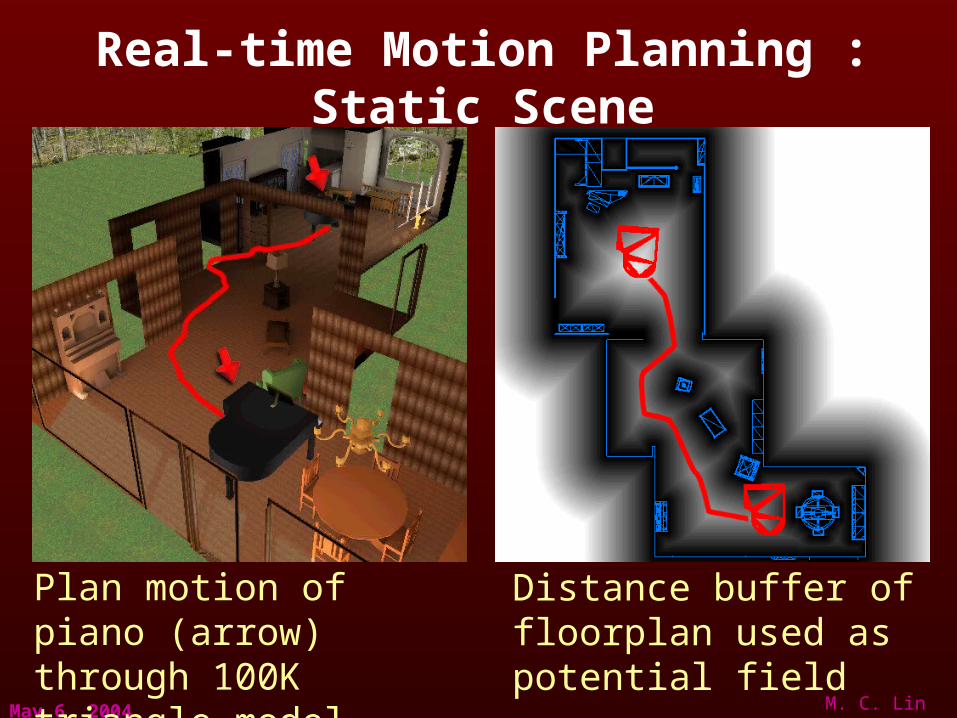
Real-time Motion Planning : Static Scene

Plan motion of piano (arrow) through 100K triangle model

Distance buffer of floorplan used as potential field

May 6, 2004 M. C. Lin

Real-time Motion Planning : Dynamic Scene

Plan motion of music stand around moving furniture

Distance buffer of floor-plan used as potential field

May 6, 2004 M. C. Lin

Voronoi-Based Sampling

• Use hardware accelerated computation of generalized Voronoi diagram (GVD) for PRM with Voronoi-based sampling

• Classify narrow passages to select different sampling strategies

• Quick collision rejection tests using hardware computed distance functions

• 25% to 10x speedup over uniform sampling on several benchmarks

[Pisula, et al, WAFR’00]

May 6, 2004 M. C. Lin

3D Benchmark (I)

May 6, 2004 M. C. Lin

3D Benchmark (II)

Model Courtesy of J-P Laumond at LAAS, Toulouse

May 6, 2004 M. C. Lin

Voronoi-Based Hybrid Planner

• Use Voronoi Graphs as the estimated path

• Use the curvature of the path to orient the robot

• When a collision occur, use random sampling to correct the estimated path

[Foskey et al, IROS’01]

May 6, 2004 M. C. Lin

Articulated Robots:Crane Complex

GVG: 138.7s

Query: 334.7s

Model courtesy Jean-Paul Laumond at CNRS

May 6, 2004 M. C. Lin

Constraint-Based Motion Planning

• Transform a motion planning problem into a constraint-based dynamic simulation

• Use GPU accelerated computation of distance fields for potential functions and quick collision rejection

• Applicable to both dynamic and static environments with moving obstacles and multiple collaborative agents

[Garber & Lin’02]

May 6, 2004 M. C. Lin

Collaborating Agents

May 6, 2004 M. C. Lin

Virtual Protoyping

May 6, 2004 M. C. Lin

DiFi: Fast 3D Distance Field Computation using GPUs

• Fast computation of global 3D distance field on uniform grid

• Exploit geometric properties• Perform geometric computations efficiently on modern

GPUs

[Sud, et al; Eurographics 2004]

May 6, 2004 M. C. Lin

Global 3D Distance Fields

Hugo Model, 17K Tris Cassini Spacecraft, 93K Tris

May 6, 2004 M. C. Lin

Geometric Properties

• Compute conservative bounds on Voronoi regions– Cull primitives for which distance functions are computed

– Clamp region of distance computation

• Exploit spatial coherence to perform incremental computations

May 6, 2004 M. C. Lin

Computations on GPU

• Rasterization hardware well suited for distance computation on 2D grid

• Sweep along an axis for computation on 3D grid

• Use HW occlusion query to detect Voronoi region bounds

• Conservative sampling to guarantee object space properties using image-precision queries

• More than one order of magnitude improvement over prior methods

May 6, 2004 M. C. Lin

Motion Planning in Dynamic Environmentsusing Distance Fields Computed on GPUs

Assembly Environment (26.9K Polys)

May 6, 2004 M. C. Lin

Summary

• Techniques to exploit graphics hardware for real-time route planning and navigation of agents on complex terrains

• Simple and easy to implement

• Applicable to both static and dynamic environments

• Extended to Voronoi-based sampling for PRM

• Core of the Voronoi-based hybrid-planner

• Central to Constrained Motion Planning

May 6, 2004 M. C. Lin

Organization

• Route Planning & Navigation

• Physically-based Simulation– Modeling of Natural Phenomena (Ice, fluid, smoke, etc)

– Interaction between Textured Surfaces

May 6, 2004 M. C. Lin

Rigid Body Dynamic Simulation on GPU

[Hoff, et al 2001]

May 6, 2004 M. C. Lin

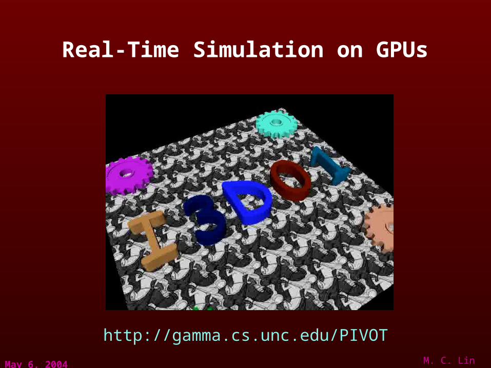
Real-Time Simulation on GPUs

http://gamma.cs.unc.edu/PIVOT

May 6, 2004 M. C. Lin

Rigid Body Dynamics on GPU

[Hoff, et al 2001]

May 6, 2004 M. C. Lin

Organization

• Route Planning & Navigation

• Physically-based Simulation– Modeling of Natural Phenomena (Ice, fluid, smoke, etc)

– Interaction between Textured Surfaces

May 6, 2004 M. C. Lin

Visual Simulation of Ice Growth

May 6, 2004 M. C. Lin

Simulation Results

Light refracting through an stained glass, as ice grows on it

May 6, 2004 M. C. Lin

Our approach

• A method for modeling and simulating visually complex structure of ice – both geometrically and optically– Physical Simulation using Phase Field Methods– Simulation Acceleration using GPUs & Banded Opt.– Controlling Complexity– Post-Processing for Rendering

[Kim and Lin, SCA’03]

May 6, 2004 M. C. Lin

Phase Field Methods

• Temperature PDE

• Phase PDE

t

pKTa

t

T

22

x

p

yy

p

xp

t

p

2

mppp

2

11

May 6, 2004 M. C. Lin

Ice Morphology

dendritic plate isotropic

May 6, 2004 M. C. Lin

GPU Acceleration

• Fields map easily to GPU• Framework of [Harris et al. 2002]

– Fields sent as textures

– Fragment program runs PDE per texel

– ~100 lines of Cg!

May 6, 2004 M. C. Lin

GPU Implementation

• To integrate PDEs– Use finite differencing for derivatives

– Integrate with forward Euler

• On GPU– finite difference = texture lookup

– Euler integration = texture add

May 6, 2004 M. C. Lin

Performance

• Only unbanded currently possible• No early exit yet on GPU

Grid Size CPU(Hz) GPU(Hz) Speedup

64x64 250 624 2.50x

128x128 25 236 9.44x

256x256 8 67.47 8.43x

512x512 3.5 17.67 5.05x

1024x1024 1.08 3.77 3.49x

1.8 GHz P-IV vs. GeForce FX 5800 Ultra

May 6, 2004 M. C. Lin

Laplacian Growth

• A computational engine and simulation framework for modeling Laplacian Growth

• Lightning, river formation, crack propagation, vegetation growth, etc.

May 6, 2004 M. C. Lin

Real-Time Capture

[Kim and Lin, SCA’03]

May 6, 2004 M. C. Lin

Fluid Simulation on GPUs

• The Navier-Stokes equations

• Plus BOUNDARY CONDITIONS• Useful for cloud/smoke/explosion simulation, modeling of

viscous paint media

May 6, 2004 M. C. Lin

GPU Implementation I

• All done with fragment programs– Textures = Grid arrays

– Fragment programs = inner loops

– Feedback (outer loops) = render to texture

• Similar to ice simulation– GPUs now better support floating point

– Richer instruction sets and HLSL

– Use Brook next

May 6, 2004 M. C. Lin

GPU Implementation II

• Most steps are simple– Most use one fragment program, one pass

– Programs come directly from equations

• Tricky parts:– Staggered grid discretization

– Boundary conditions

– Stable Fluids projection step (step 4)

May 6, 2004 M. C. Lin

Project Step & Numerical Methods

• Enforces divergence-free velocity– Iterative solution of Poisson equation

• Iterative solver options – Conjugate Gradient

– Multigrid

– Gauss-Seidel, SOR

– FFT

– Jacobi, Red-Black Gauss Seidel

May 6, 2004 M. C. Lin

Organization

• Route Planning & Navigation

• Physically-based Simulation– Modeling of Natural Phenomena (Ice, fluid, smoke, etc)

– Interaction between Textured Surfaces

May 6, 2004 M. C. Lin

Haptic Texture Rendering

• The Challenge: haptic rendering of interaction between textured models (target: 1kHz)– Collision detection between complex models is prohibitive

– Simplified objects: texture effects are missed

May 6, 2004 M. C. Lin

Novel Approach

• 2-step process1) Compute contact information between low-resolution models

(as presented by Otaduy and Lin, SIGGRAPH 2003)

2) Refine penetration depth with texture-mapping approach (GPU implementation) and compute force and torque.

May 6, 2004 M. C. Lin

Texture Force Computation

• Force based on gradient of penetration depth (δ)

(F T)T=-kδ (∂δ/∂u ∂δ/∂v 1 ∂δ/∂θu ∂δ/∂θv ∂δ/∂θn)T

δn

u

May 6, 2004 M. C. Lin

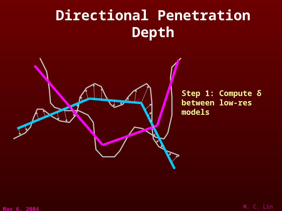
Directional Penetration Depth

Example of 2 intersecting objects

May 6, 2004 M. C. Lin

Directional Penetration Depth

Penetration depth (δ): minimum distance to make the objects disjoint

May 6, 2004 M. C. Lin

Directional Penetration Depth

May 6, 2004 M. C. Lin

Directional Penetration Depth

May 6, 2004 M. C. Lin

Directional Penetration Depth

May 6, 2004 M. C. Lin

Directional Penetration Depth

May 6, 2004 M. C. Lin

Directional Penetration Depth

Novel approach: represent models by…

May 6, 2004 M. C. Lin

Directional Penetration Depth

Novel approach: represent models by…

Low-res models

May 6, 2004 M. C. Lin

Directional Penetration Depth

Novel approach: represent models by…

Low-res models

+ Texture detail

May 6, 2004 M. C. Lin

Directional Penetration Depth

Step 1: Compute δ between low-res models

May 6, 2004 M. C. Lin

Directional Penetration Depth

May 6, 2004 M. C. Lin

Directional Penetration Depth

May 6, 2004 M. C. Lin

Directional Penetration Depth

May 6, 2004 M. C. Lin

Directional Penetration Depth

δ sets the penetration direction n

n

May 6, 2004 M. C. Lin

Directional Penetration Depth

Step 2: Refine directional penetration depth based on texture detail

n

May 6, 2004 M. C. Lin

Directional Penetration Depth

GPU implementation: discretized + parallel computation

n

May 6, 2004 M. C. Lin

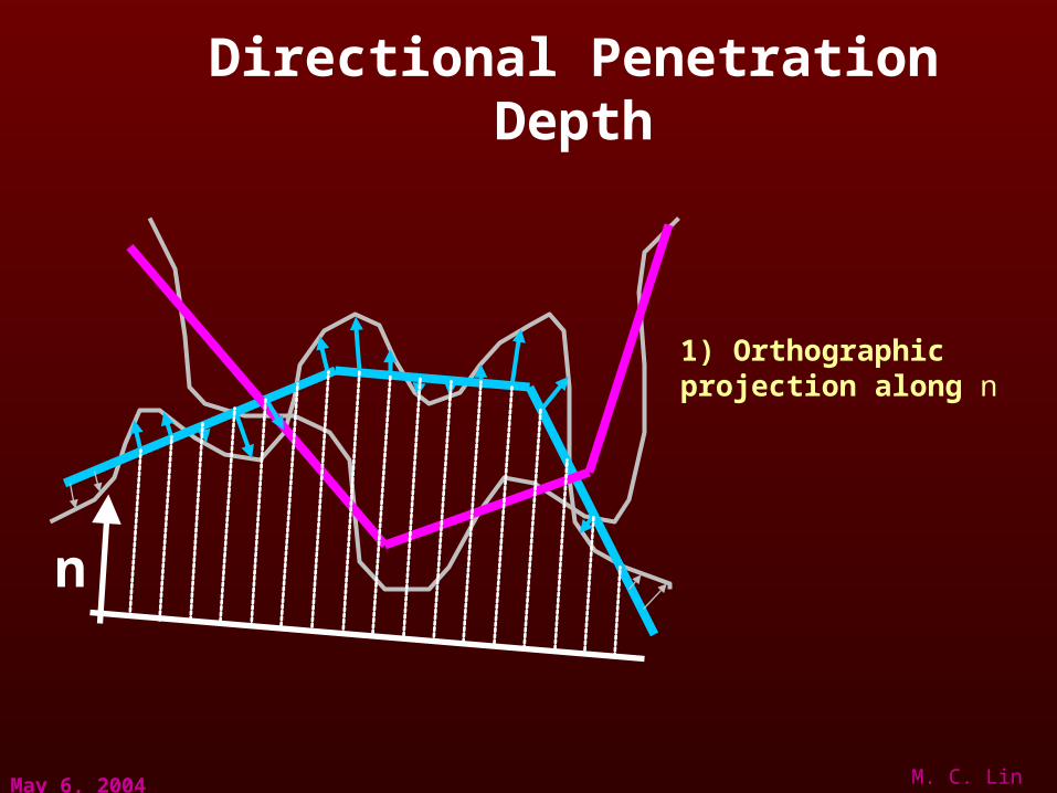
Directional Penetration Depth

1) Orthographic projection along n

n

May 6, 2004 M. C. Lin

Directional Penetration Depth

2) In fragment program, query texture map to obtain fine-detail positions

n

May 6, 2004 M. C. Lin

Directional Penetration Depth

3) Store height field in texture memory

n

May 6, 2004 M. C. Lin

Directional Penetration Depth

4) Copy height field difference to depth buffer

n

May 6, 2004 M. C. Lin

Directional Penetration Depth

5) Search for max difference = penetration depth

n

δn

May 6, 2004 M. C. Lin

Why GPUs?

• Parallelized computation

• Many subparts of the algorithm map naturally to graphics hardware

– Orthographic projection

– Texture mapping

– Fast max search based on occlusion queries (Govindaraju et al., SIGMOD 2004) to avoid read-backs.

May 6, 2004 M. C. Lin

Future Work on GPUs

• Extension to route planning with visibility constraints, among multiple agents, or for deformable/reconfigurable robots

• Real-time physically-based modeling and simulation of natural phenomena (sand storms, smokes, rain/ice, etc.)

• Interactive simulation of interaction between complex objects using “geometry textures”

May 6, 2004 M. C. Lin

Collaborator & Students

Dinesh Manocha

Bill BaxterTim Culver

Mark FoskeyMaxim Garber

Kenny HoffJohn Keyser

Theodore KimMiguel OtaduyCharles Pisula

May 6, 2004 M. C. Lin

The End

May 6, 2004 M. C. Lin

GPU Implementation

• Set a 1:1 mapping from pixels to texels:– Set view port resolution to texture resolution.– Use orthographic projection.

• To sample an immediate neighbor of each texel:– Draw a single quad filling the view port.– Set texture coordinates at corners to {(0,0), (0,1), (1,1), (1,0)} plus the

offset to the neighbor.• E.G. Offset to right is (w, 0), where is view space texel width.

May 6, 2004 M. C. Lin

GPU Implementation I

Velocity

PenetrationDepth

Volume

AdvectedScalars

GPU FP Fragment Processors

GPU VP Vertex Processors

Collision MeshTextures

May 6, 2004 M. C. Lin

GPU Implementation II

FP

VP VP

FP FP FP FPMain GPUUnits Used

TexturesWritten

TexturesRead

Volume

PD Velocity

PD PD, Velocity PD PDScalarsVolume

ScalarsVolume

Scalars

Scalars

Scalars

Scalars