1

Maximum Principle for Survey Data Analysis * J. E. Mullat **

Abstract. The note addresses a principle of data cleaning. An implementation procedure of the principle contains a recommendation that might be well suited for clarifying and illustrating the results of survey data analysis.

1. Introduction

Surveys, studies, statistics, opinions measurements, research results, etc. are served to us on a daily basis, in an infinite stream and are used both by enterprises, media-experts, universities and other organizations to tell us something about reality – how things works. But, has anyone questioned this way of having reality served on a platter? Most people merely accept what the various analysts have presented. Thus, if more people in a survey have answered that they prefer rye bread to the white bread, is it true for the world in general? Must we conclude that people in general eat more rye bread instead of white? Certainly not. Reality is complex and consists of numerous choices, possibilities, behavioral patterns, preferences, etc. A regular survey cannot cover all relevant data appertaining to any given subject and can more often than not lead to completely nonsensical conclusions. Closer approximations will often require a comprehensive statistical investigation. Therefore, as a rule, one should turn to a researcher or some other qualified person to make a statement regarding the qualitative content of the numerous variables disposed in the background so that the results can be interpreted and analyzed. Additionally, it is essential not to waive our personal estima-tion of the researcher’s knowledge and expertise and whether the questions discussed lie in the field of the respondents’ credibility, in other words, the designated reliability.

2. Reliability

Reliability might seem to be a concept, which is almost impossible to define. Nevertheless, we can show that the “maximum principle” will not only help the researcher in his/her analytical role, but also “clean up” the investigation, filtering out the more “unreliable” answers and in this manner remove some “interference”, that is, the respondents, whose answers lie distant from the most conceivable result. However, it must be emphasized that the role of the analysis is still central and in spite of this angle of the argument, the final estimation should still be based on the subjective perception of reality. After all, the primary difference between this method and the

* Presented at the 19th Nordic Conference on Mathematical Statistics, June 9-13, 2002, Stockholm, Sweden

and at the Symposium i Advent Statistik, 23-26 januar 2006, København. ** Byvej 269, 2650 Hvidovre, Denmark, mailto: jm@mail-telia.dk

2

conventional statistical analysis of a survey, is that our methods sorts out unreliable respondents together with their unreliable answers. Consequently, we hereby obtain rather sharper picture of reality simply by looking at patterns agreeing with the rest of the answers in the group. We will now exemplify the method, going an exemplified survey in progress. We emphasize that what follows is significantly simplified in order to set up the foundations of the method.

Food is an area, which frequently comes under the analyst’s loop. So, let us assume that we are trying to map people’s taste preferences. We have decided to ask respondents about five definite menus and from this people’s daily usage.

These menus consist of: 1. Dairy produce: cheese and milk 2. Cereals: bread, potatoes, rise and pasta 3. Vegetables: vegetables, fruit, etc. 4. Fish: shrimps, frozen/fresh fish 5. Meat products: various meats, sandwich spreads and sausages

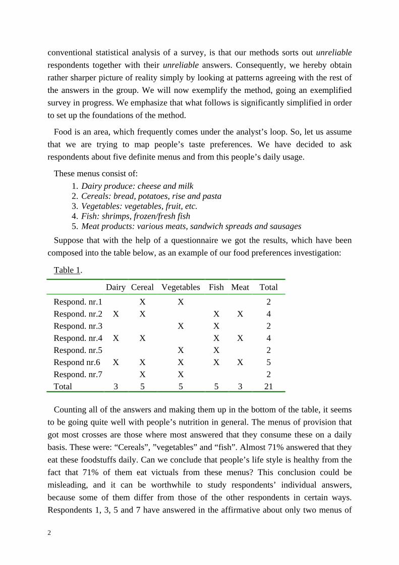
Suppose that with the help of a questionnaire we got the results, which have been composed into the table below, as an example of our food preferences investigation:

Table 1.

Dairy Cereal Vegetables Fish Meat Total

Respond. nr.1 X X 2 Respond. nr.2 X X X X 4 Respond. nr.3 X X 2 Respond. nr.4 X X X X 4 Respond. nr.5 X X 2 Respond nr.6 X X X X X 5 Respond. nr.7 X X 2 Total 3 5 5 5 3 21

Counting all of the answers and making them up in the bottom of the table, it seems to be going quite well with people’s nutrition in general. The menus of provision that got most crosses are those where most answered that they consume these on a daily basis. These were: “Cereals”, ”vegetables” and “fish”. Almost 71% answered that they eat these foodstuffs daily. Can we conclude that people’s life style is healthy from the fact that 71% of them eat victuals from these menus? This conclusion could be misleading, and it can be worthwhile to study respondents’ individual answers, because some of them differ from those of the other respondents in certain ways. Respondents 1, 3, 5 and 7 have answered in the affirmative about only two menus of

3

goods. Respondents nr. 1 and 7 consume “cereals” and ”vegetable” products, while nr. 3 and 5 consume only ”vegetables” and “fish”. Assuming that this is the whole nutrition foundation (again, note the simplifications in this example), it seems some-what abnormal eat from only these two food groups. And this is central: we believe that the answers of respondents like these are unreliable reflections of reality. Let us therefore experimentally discard the unreliable respondents together with their answers to see whether we obtain a different result – a more credible result, closer to reality.

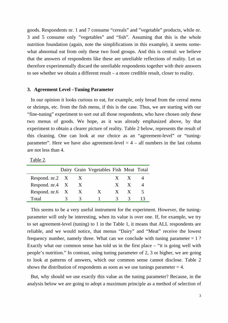
3. Agreement Level –Tuning Parameter

In our opinion it looks curious to eat, for example, only bread from the cereal menu or shrimps, etc. from the fish menu, if this is the case. Thus, we are starting with our “fine-tuning” experiment to sort out all those respondents, who have chosen only these two menus of goods. We hope, as it was already emphasized above, by that experiment to obtain a clearer picture of reality. Table 2 below, represents the result of this cleaning. One can look at our choice as an “agreement-level” or “tuning-parameter”. Here we have also agreement-level = 4 – all numbers in the last column are not less than 4.

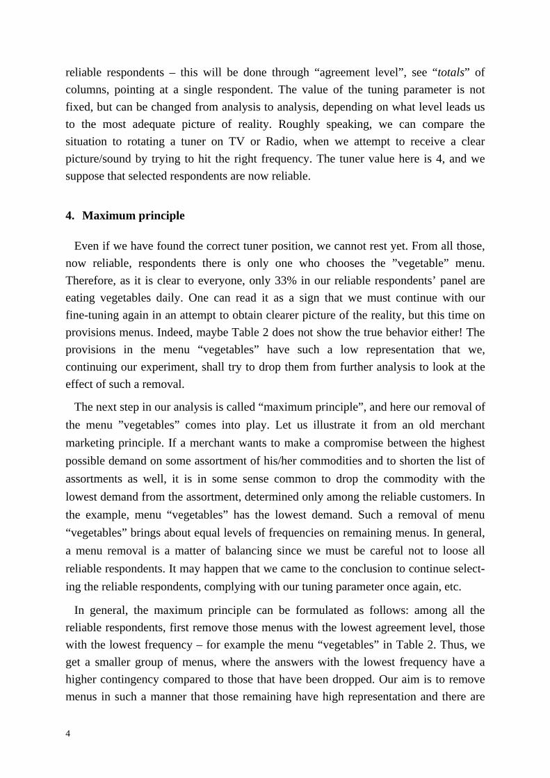
Table 2.

Dairy Grain Vegetables Fish Meat Total

Respond. nr.2 X X X X 4 Respond. nr.4 X X X X 4 Respond. nr.6 X X X X X 5 Total 3 3 1 3 3 13

This seems to be a very useful instrument for the experiment. However, the tuning-parameter will only be interesting, when its value is over one. If, for example, we try to set agreement-level (tuning) to 1 in the Table 1, it means that ALL respondents are reliable, and we would notice, that menus “Dairy” and “Meat” receive the lowest frequency number, namely three. What can we conclude with tuning parameter = 1 ? Exactly what our common sense has told us in the first place – “it is going well with people’s nutrition.” In contrast, using tuning parameter of 2, 3 or higher, we are going to look at patterns of answers, which our common sense cannot disclose. Table 2 shows the distribution of respondents as soon as we use tunings parameter = 4.

But, why should we use exactly this value as the tuning parameter? Because, in the analysis below we are going to adopt a maximum principle as a method of selection of

4

reliable respondents – this will be done through “agreement level”, see “totals” of columns, pointing at a single respondent. The value of the tuning parameter is not fixed, but can be changed from analysis to analysis, depending on what level leads us to the most adequate picture of reality. Roughly speaking, we can compare the situation to rotating a tuner on TV or Radio, when we attempt to receive a clear picture/sound by trying to hit the right frequency. The tuner value here is 4, and we suppose that selected respondents are now reliable.

4. Maximum principle

Even if we have found the correct tuner position, we cannot rest yet. From all those, now reliable, respondents there is only one who chooses the ”vegetable” menu. Therefore, as it is clear to everyone, only 33% in our reliable respondents’ panel are eating vegetables daily. One can read it as a sign that we must continue with our fine-tuning again in an attempt to obtain clearer picture of the reality, but this time on provisions menus. Indeed, maybe Table 2 does not show the true behavior either! The provisions in the menu “vegetables” have such a low representation that we, continuing our experiment, shall try to drop them from further analysis to look at the effect of such a removal.

The next step in our analysis is called “maximum principle”, and here our removal of the menu ”vegetables” comes into play. Let us illustrate it from an old merchant marketing principle. If a merchant wants to make a compromise between the highest possible demand on some assortment of his/her commodities and to shorten the list of assortments as well, it is in some sense common to drop the commodity with the lowest demand from the assortment, determined only among the reliable customers. In the example, menu “vegetables” has the lowest demand. Such a removal of menu “vegetables” brings about equal levels of frequencies on remaining menus. In general, a menu removal is a matter of balancing since we must be careful not to loose all reliable respondents. It may happen that we came to the conclusion to continue select-ing the reliable respondents, complying with our tuning parameter once again, etc.

In general, the maximum principle can be formulated as follows: among all the reliable respondents, first remove those menus with the lowest agreement level, those with the lowest frequency – for example the menu “vegetables” in Table 2. Thus, we get a smaller group of menus, where the answers with the lowest frequency have a higher contingency compared to those that have been dropped. Our aim is to remove menus in such a manner that those remaining have high representation and there are

5

more matches in their answers. In other words, the menu, where the matching is low, the low match is relatively high, due to the removal, which would not be the case if the removed menus will still occupy a place in the table. So, the aim is not only to separate a group of menus from the rest, which have higher matching responses, but also to find a group of respondents, where the menu with the lowest level of matching is on a relative high level. This is the central for understanding the maximum principle. Not only must the respondents be reliable, but also answers producing such reliability must be more or less identical.

In accordance with Table 2 we take menu “vegetables” out, since it falls apart from the general answer pattern due to our maximum principle. Note that here we estimate not from the qualitative basis, but purely on a pattern disclosed by matching answers matching!

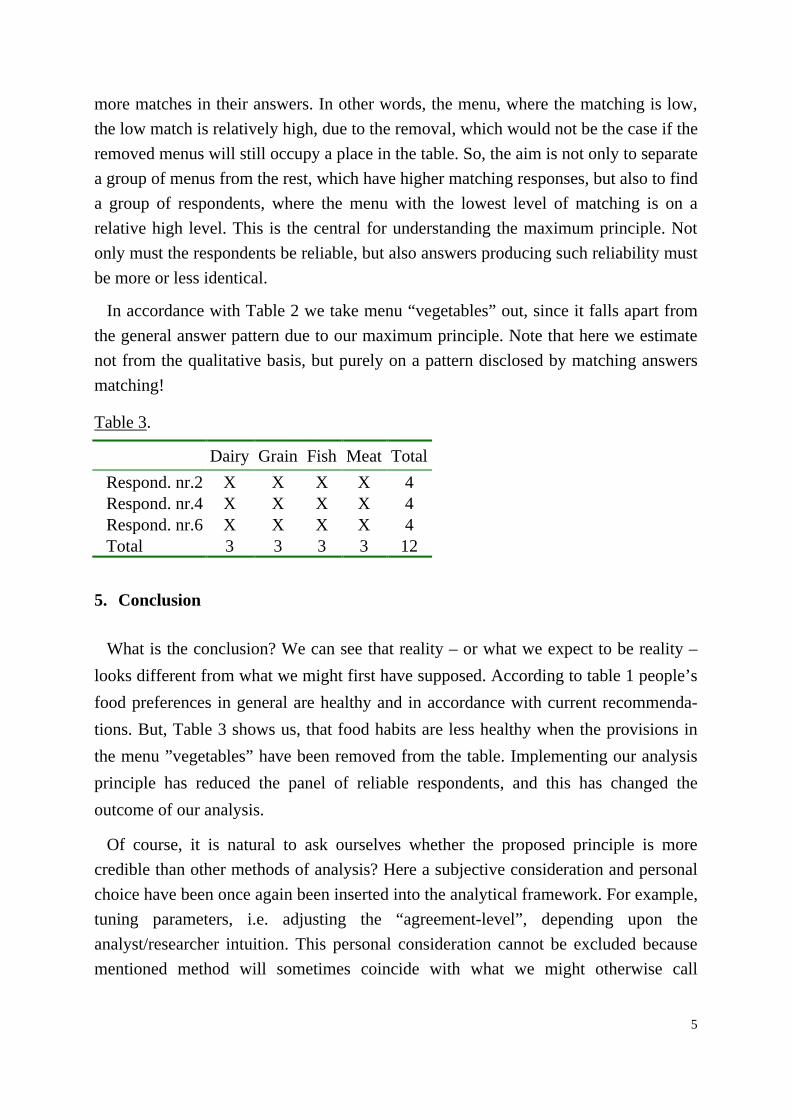
Table 3.

Dairy Grain Fish Meat TotalRespond. nr.2 X X X X 4 Respond. nr.4 X X X X 4 Respond. nr.6 X X X X 4 Total 3 3 3 3 12

5. Conclusion

What is the conclusion? We can see that reality – or what we expect to be reality – looks different from what we might first have supposed. According to table 1 people’s food preferences in general are healthy and in accordance with current recommenda-tions. But, Table 3 shows us, that food habits are less healthy when the provisions in the menu ”vegetables” have been removed from the table. Implementing our analysis principle has reduced the panel of reliable respondents, and this has changed the outcome of our analysis.

Of course, it is natural to ask ourselves whether the proposed principle is more credible than other methods of analysis? Here a subjective consideration and personal choice have been once again been inserted into the analytical framework. For example, tuning parameters, i.e. adjusting the “agreement-level”, depending upon the analyst/researcher intuition. This personal consideration cannot be excluded because mentioned method will sometimes coincide with what we might otherwise call

6

common sense, where the most frequent answers reflect the actual reality. This should be the case, when dealing with simple surveys, for example, “will you vote for so and so the coming election?” and the like.

What if we have to deal with more complicated surveys with hundreds or thousands of respondents and many hundreds of questions? It will automatically generate so complicated tables and patterns that “common sense” will be impossible to wield, since unaided human intellect is incapable of grasping such complicated patterns. This is where our method comes efficiently into play, because it is a way of locating erroneous or out of place patterns, based on comparison within the data. The analyst role is not yet outplayed, since it is up to him or her to make the relevant judgments/decisions as to why data is discounted? The essence is, that we try to filter out all “unreliable” respondents with the help of our “tuning parameter”. In this “cleansing procedure” we try to find the most usable answers setting up our maximum principle. It should be seen as an instrument, which has to be used correctly by the analyst to tune into the clearest reality. The aim is to reduce the jamming effect produced by unreliable respondents.

Appendix

A.1 Practical recommendations

The preliminary explanation above is a general introduction to our maximum principle, which has a background in a much more complicated methodology and theory. 1 First let’s have a look at, how the results can be used and illustrated for the analyst – there are some basic lines, which can simplify the work by weeding in the data. This is where a notion of positive/negative profile comes into consideration.

Constructing a questionnaire, the questions should be in order – in the “same direc-tion” through the whole questionnaire – always going from some positive to negative answers (values/opinions) or vice versa. In a more rigorous vocabulary we call such ordering an ordinal scale. This is primarily, because a in computer implementation, using our method, the analyst must separate the answers by grouping them together into positive/negative scale ends – the (+/–)-pools. The next step will be to create profile groups within each (+)- or (–)-pool range. A profile group of answers is put together following their subject-oriented field of interest. For example, one might be interested in life style, or in a profile that concerns nutrition practice, or a profile about 1 Some theoretical aspects may be found in the appendix A.2

7

exercising, etc. Thus, these profiles, distinguished by their placement in (+/–)-pools, are also either positive or negative.

Now the analyst has some arrangement of (+/–)-profiles, as he created them. From hereon it is no longer the task of the analyst to proceed with the analysis, but an automated process utilizing our maximum principle, which further organizes the data into what we call a series of profile components. Each profile components is a table, as above, lying within particular profile limits. The difference between a component and the profile clearly is that, while a profile is a list of subject-oriented questions – options/answers composed by the analyst, the component is a table composed with the maximum principle. Therefore, the list of answers constituting a component (now the set of table columns in a table) is smaller – it is only some answers/columns, which constitutes the profile. Thus, once again the components will be separated into

(+/–)-components ,...K,K ±±21 as until now the profiles were separated into

(+/–)-profiles. The purpose of ,...K,K ±±21 separation besides conceptual advantages

lies also in the illustration opportunities.

It is no secret that illustration is an essential part of the analysis. The simplest tool available is a pie chart. Here we may divide the pie into our (green) – positive

,...K,K ++21 , and (red) – negative ,...K,K −−

21 components found. However, we must

calculate some statistical parameters beforehand. For example, one can merge the (+/–)-components into single (+/–)-table and calculate the (+/–)-probabilities2. Hereby, statistical parameters based on (+/–)-probabilities may be evaluated and illustrated by a pie divided into green and red area – consequently the (+/–)-areas3. There are a lot of techniques and graphical tools available, and a creative analyst may proceed in this direction indefinitely. Nevertheless, one may ask the question why all this trouble with the (+/–)-components? Why not implement the same illustration technique on the survey data without any “maximum principle”? The answer is the blurred nature of the data may hinder clear interpretation of the reality underlying the data, see above.

2 Certainly, some estimates only. 3 Please, find below a pie typical to what we just discussed. The positive and negative profiles are 21 questions highlighting

people’s behaviour, responses, opinions, etc. regarding their daily work. Answers of the questions impersonate an ordinal scale 1,2,...5 , where 1,2,3 is negative, and 3,4,5 – positive scale ends.

8

A.2 Some theoretical aspects

Suppose that respondents n,...i,...,N 1= participate in the survey. Let x , Nx 2∈ , be

those who expressed their preferences towards certain questions m,...,j,...,M 1= .

We lose no generality in looking at list M as at the profile – negative or positive. Let

a Boolean table m

nijaW = reflect the survey result of respondents’ preferences; 1=ija

if respondent i prefers the answer j , 0=ija if not. Also all lists M2 of answers My 2∈ within a profile M have been examined. Let an index 0=k

ijδ , yj,xi ∈∈ if

∑ ∈ <yj ij ka , otherwise 1=kijδ , e.g. ∑ ∈ ≥yj ij ka , where k is our tuning parameter.

We can calculate an indicator )H(Fk using sub-table H on crossing entries of the

rows x and columns y in the original table W . The number of 1-entries 1=⋅ ijkij aδ in

each column within the range y determines the indicator )H(Fk by further selection

of a column with the least – the minimum number )H(Fk from the list y .

In order to find a component K seems tautological in the sense that following our maximum principle we have to solve the indicator maximization problem

)H(FmaxargK k)y,x(= . The task, one might wonder, is a NP-hard problem to solve

with the number of operations growing exponentially. Fortunately, we claim that our ±K components might be found by polynomial )nlognm(O 2⋅⋅ algorithm, see in the

literature. Finally, we can restructure the whole procedure by consequentially

extracting a component ±1K first, then removing it from the original table W and

repeating the extraction procedure on the rest obtaining components ±2K , ±

3K ,... etc.

From now on, statistical parameters and its like, which empower (+/–)-share only from

components ,...K,K −−21 and ,...K,K ++

21 , are available to the analyst for illustration

purposes, see example below.

References

Mullat, J.E., A Fast Algorithm for Finding Matching Responses in a Survey Data Table, Mathematical Social Sciences, 1995, 30, 195 – 205. http://www.sciencedirect.com/science/article/B6V88-3YMFS06-13/2/2789968ef01b5eaed9534ad2b6a79147

9

A.3 Illustration

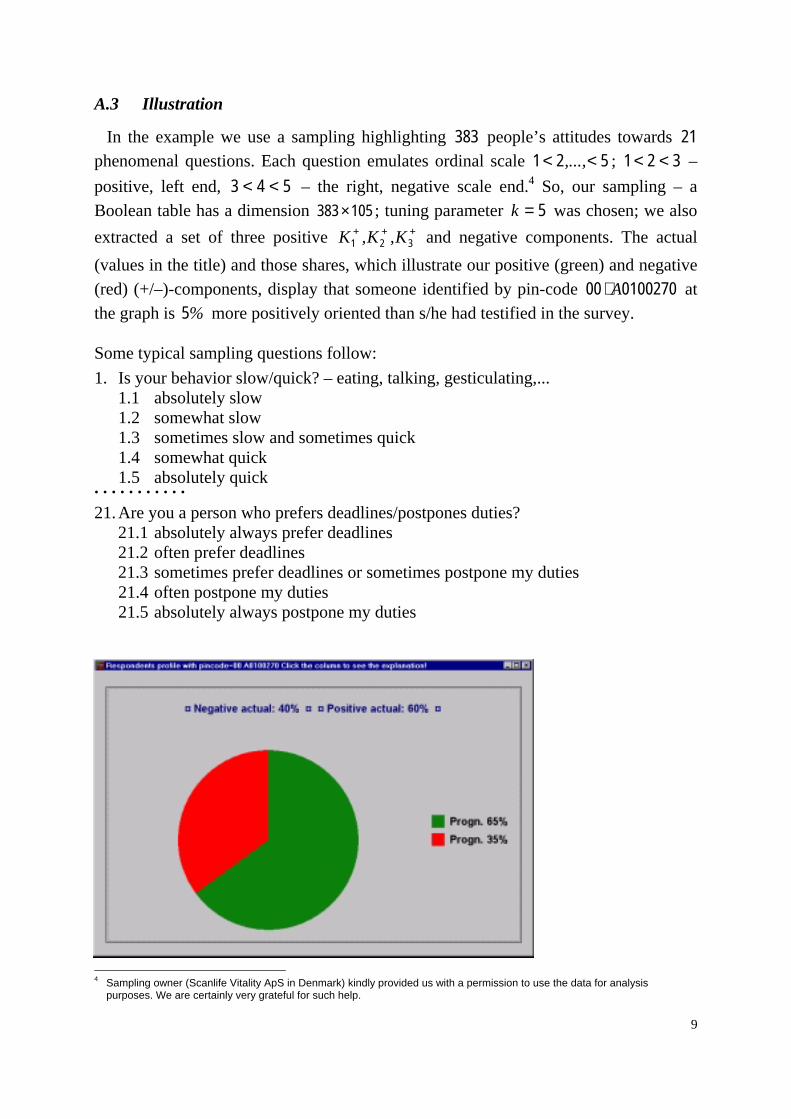
In the example we use a sampling highlighting 383 people’s attitudes towards 21 phenomenal questions. Each question emulates ordinal scale 521 << ,..., ; 321 << – positive, left end, 543 << – the right, negative scale end.4 So, our sampling – a Boolean table has a dimension 105383× ; tuning parameter 5=k was chosen; we also extracted a set of three positive +++

321 K,K,K and negative components. The actual (values in the title) and those shares, which illustrate our positive (green) and negative (red) (+/–)-components, display that someone identified by pin-code 010027000 A⋅ at the graph is %5 more positively oriented than s/he had testified in the survey.

Some typical sampling questions follow: 1. Is your behavior slow/quick? – eating, talking, gesticulating,... 1.1 absolutely slow 1.2 somewhat slow 1.3 sometimes slow and sometimes quick 1.4 somewhat quick 1.5 absolutely quick . . . . . . . . . . . 21. Are you a person who prefers deadlines/postpones duties?

21.1 absolutely always prefer deadlines 21.2 often prefer deadlines 21.3 sometimes prefer deadlines or sometimes postpone my duties 21.4 often postpone my duties 21.5 absolutely always postpone my duties

4 Sampling owner (Scanlife Vitality ApS in Denmark) kindly provided us with a permission to use the data for analysis

purposes. We are certainly very grateful for such help.

Mathematical Social Sciences 30 (1995) 195-205 North-Holland, ELSEVIER. We alert the readers’ obligation with respect to copyrighted material.

1

A fast algorithm for finding matching responses in a survey data table *

Joseph E. Mullat

Byvej 269, 2650 Hvidovre, Copenhagen, Denmark **

Abstract

The paper addresses an algorithm to perform an analysis on survey data tables with some irreliable entries. The algo-rithm has almost linear complexity depending on the number of elements in the table. The proposed technique is based on a monotonicity property. An implementation procedure of the algorithm contains a recommendation that might be realistic for clarifying the analysis results.

Keywords: Survey; Boolean; Data Table; Matrix.

1. Introduction

Situations in which customer responses being studied are measured by means of survey

data arise in the market investigations. They present problems for producing long-term

forecasts because the traditional methods based on counting the matching responses in the

survey with a large customer population are hampered by unreliable human nature in the

answering and recording process. Analysis institutes are making considerable and expen-

sive efforts to overcome this uncertainty by using different questioning techniques, includ-

ing private interviews, special arrangements, logical tests, “random” data collection, ques-

tionnaire scheme preparatory spot tests, etc. However, percentages of responses represent-

ing the statistical parameters rely on misleading human nature and not on a normal distri-

bution. It appears thereby impossible to exploit the most simple null hypothesis technique

because the distributions of similar answers are unknown. The solution developed in this

paper to overcome the hesitation effect of the respondent, and sometimes unwillingness,

rests on the idea of searching so-called “agreement lists” of different questions. In the

agreement list, a significant number of respondents do not hesitate in choosing the identi-

cal answer options, thereby expressing their willingness to answer. These respondents and

the agreement lists are classified into some two-dimensional lists – "highly reliable

blocks".

* The idea explained also in http://www.datalaundering.com/download/cleaning.pdf appears to be clear for those indif-ferent to higher level of abstraction.

** Residence in Denmark since 1980, Ph.D. in computer science, assoc. Prof., economic division, Tallinn Technical University, Estonia (from 1979 - 1980).

2 J. E. Mullat / Mathematical Social Sciences 30 (1995) 195-205

For survey analysts with different levels of research experience, or for the people

mostly interested in receiving results by their methods, or merely for those who are famil-

iar with only one, "the best survey analysis technique", our approach has some advantages.

Indeed, in the survey, data are collected in such a way that can be regarded as respondents

answering a series of questions. A specific answer is an option such as displeased, satis-

fied, well contented, etc. Suppose that all respondents participating in the survey have been

interviewed using the same questionnaire scheme. The resulting survey data can then be arranged in a table ⟩⟨= qixX , where qix is a Boolean vector of options available, while

the respondent i is answering the question q. In this respect, the primary table X is a col-

lection of Boolean columns where each column in the collection is filled with Boolean

elements from only one particular answer option. Our algorithm will always try to detect

some highly reliable blocks in the Table X bringing together similar columns, where only

some trustworthy respondents are answering identically. Detecting these blocks, we can

separate the survey data. Then, we can reconstruct the data back from those blocks into the primary survey data table ⟩′⟨=′ qixX format, where some "non-matching/ doubtful" an-

swers are removed. Such a "data-switch" is not intended to replace the researchers’ own

methods, but may be complementary used as a "preliminary data filter” - separator. The

analysts’ conclusions will be more accurate after the data-switch has been done because

each filtered data item is a representative for some "well known subtables".

Our algorithm in an ordinary form dates back to Mullat (1971). At first glance, the ordi-

nary form seems similar to the greedy heuristic (Edmonds 1971), but this is not the case.

The starting point for the ordinary version of the algorithm is the entire table from which

the elements are removed. Instead, the greedy heuristic starts with the empty set, and the

elements are added until some criterion for stopping is fulfilled. However, the algorithm

developed in the present paper is quite different. The key to our paper is that the properties

of the algorithm remain unchanged under the current construction. For matching responses

in the Boolean table, it has a lower complexity.

J. E. Mullat / Mathematical Social Sciences 30 (1995) 195-205 3

The monotone property of the proposed technique - “monotone systems idea” - is a

common basis for all theoretical results. It is exactly the same property (iii) of submodular

functions brought up by Nemhauser et al. (1978, p.269). Nevertheless, the similarity does

not itself diminish the fact that we are studying an independent object, while the property

(iii) of submodular set functions is necessary, but not sufficient.

From the very start, the theoretical apparatus called the "monotone system" has been

devoted to the problem of finding some parts in a graph that are more "saturated" than any

other part with "small" graphs of the same type (see Mullat, 1976). Later, the graph presen-

tation form was replaced by a Markov chain where the rows-columns may be split imple-

menting the proposed technique into some sequence of submatrices (see Mullat, 1979).

There are numerous applications exploiting the monotone systems ideas; see Ojaveer et al.

(1975). Many authors have developed a thorough theoretical basis extending the original

conception of the algorithm; see Libkin et al. (1990) and Genkin and Muchnik (1993).

The rest of the paper is organized as follows. In SSeeccttiioonn 22, a reliability criterion will be

defined for blocks in the Boolean table B . This criterion guarantees that the shape of the

top set of our theoretical construction is a submatrix - a block; see the PPrrooppoossiittiioonn 11. How-

ever, the point of the whole monotone system idea is not limited by our specific criterion

as described in SSeeccttiioonn 22. This idea addresses the question: How to synthesize an analysis

model for data matrix using quite simple rules? In order to obtain a new analysis model,

the researcher has only to find a family of π -functions suitable for the particular data. The

shape of top sets for each particular choice of the family of π -functions might be different;

see the note prior to our formal construction. For practical reasons, especially in order to

help the process of interpretation of the analysis results, in SSeeccttiioonn 33 there are some rec-

ommendations on how to use the algorithm on the somewhat extended Boolean tables ±B .

SSeeccttiioonn 44 is devoted to an exposition of the algorithm and its formal mathematical proper-

ties, which are not yet utilized widely by other authors.

4 J. E. Mullat / Mathematical Social Sciences 30 (1995) 195-205

2. Reliability Criterion

In this Section we deal with the criterion of reliability for blocks in the Boolean tables

originating from the survey data. In our case we analyze the Boolean table ⟩⟨= jibB rep-

resenting all respondents ⟩⟨ n,...,i,..., 1 , but including only some columns ⟩⟨ m,...j,...,1

from the primary survey data table ⟩⟨= qixX ; see above. The resulting data of each table

B can be arranged in a mn × matrix. Those Boolean tables are then subjected to our algo-

rithm separately, for which reason there is no difference between any subtable in the pri-

mary survey data and a Boolean table. A typical example is respondent satisfaction with

services offered, where 1 =jib if respondent i is satisfied with a particular service j

level, and 0 =jib if he is unsatisfied. Thus, we analyze any Boolean table of the survey

data independently.

Let us find a column j with the most significant frequency F of 1-elements among all

columns and throughout all rows in table B . Such rows arrange a 1=g one column subt-

able pointing out only those respondents who prefer one specific most significant column j.

We will treat, however, a more general criterion. We suggest looking at some significant

number of respondents where at least F of them are granting at least g Boolean

1-elements in each single row within the range of a particular number of columns. Those

columns arrange what we call an agreement list, ,...,g 32= ; g is an agreement level.

The problem of how to find such a significant number of respondents, where the F cri-

terion reaches its global maximum, is solved in SSeeccttiioonn 44. An optimum table *S , which

represents the outcome of the search among all “subsets” H in the Boolean table B , is the

solution; see Theorem I. The main result of the Theorem I ensures that there are at least F

positive responses in each column in table *S . No superior subtable can be found where

the number of positive responses in each column is greater than F . Beyond that, the

agreement level is at least equal to ,...,g 32= in each row belonging to the best subtable

*S ; g is the number of positive responses within the agreement list represented by col-

J. E. Mullat / Mathematical Social Sciences 30 (1995) 195-205 5

umns in subtable *S . In case of an agreement level 1=g , our algorithm in SSeeccttiioonn 44 will

find out only one column j with the most significant positive frequency F among all col-

umns in table B and throughout all respondents, see above. Needless to say that it is

worthless to apply our algorithm in that particular case 1=g , but the problem becomes

fundamental as soon as ,...,g 32= .

Let us look at the problem more closely. The typical attitude of the respondents towards

the entire list of options - columns in table B can be easily "accumulated" by the total

number of respondent i positive hits - options selected:

∑=

=m,...,j

jii br1

.

Similarly, each column - option can be measured by means of the entire Boolean table B

as

∑=

=n,...,i

jij bc1

.

It might appear that it should be sufficient to choose the whole table B to solve our

problem provided that n,...,i,gri 1=≥ . Nevertheless, let us look throughout the whole

table and find the worse case where the number m,...,j,c j 1= reaches its minimum F .

Strictly speaking, it does not mean that the whole table B is the best solution just because

some "poor" columns (options with rare responses - hits) may be removed in order to raise

the worst-case criterion F on the remaining columns. On the other hand, it is obvious that

while removing "poor" columns, we are going to decrease some ir numbers, and now it is

not clear whether in each row there are at least ,...,g 32= positive responses. Trying to

proceed further and removing those "poor" rows, we must take into account that some of

jc numbers decrease and, consequently, the F criterion decreases as well. This leads to

the problem of how to find the optimum subtable *S , where the worst case - F criterion

reaches its global maximum? The solution is in SSeeccttiioonn 44.

6 J. E. Mullat / Mathematical Social Sciences 30 (1995) 195-205

Finally, we argue that the intuitively well adapted model of 100% matching 1-blocks is

ruled out by any approach trying to qualify the real structure of the survey data. It is well

known that the survey data matrices arising from questionnaires are fairly empty. Those

matrices contain plenty of small 100% matching 1-blocks, whose individual selection

makes no sense. We believe that the local worst case criterion F top set, found by the al-

gorithm, is a reasonable compromise. Instead of 100% matching 1-blocks, we detect

somewhat blocks less than 100% filled with 1-elements, but larger in size.

3. Recommendations

We consider the interpretation of the survey analysis results as an essential part of the

research. This Section is designed to give a guidance on how to make the interpretation

process easier. In each survey data it is possible to conditionally select two different types

of questions: (1) The answer option is a fact, event, happening, issue, etc.; (2) The answer

is an opinion, namely displeased, satisfied, well contented etc.; see above. It does not ap-

pear from the answer to options of type 1, which of them is positive or negative, whereas

type 2 allows us to separate them. The goal behind this splitting of type 2 opinions is to

extract from the primary survey data table two Boolean subtables: table +B , which in-

cludes type 1 options mixed with the positive options from type 2 questions, and table −B

where type 1 options are mixed together with the negative type 2 options - opinions. It

should be noticed that doing it this way, we are replacing the analysis of primary survey

data by two Boolean tables where each option is represented by one column. Tables +B

and −B are then subjected to the algorithm separately.

To initiate our procedure, we construct a subtable +1K implementing the algorithm on

table +B . Then, we replace subtable +1K in +B by zeros, constructing a restriction of ta-

ble ±B . Next, we implement the algorithm on this restriction and find a subtable +2K , after

which the process of restrictions and subtables sought by the algorithm may be continued.

For practical purposes we suggest stopping the extraction with three subtables: +1K , +

2K

and +3K . We can use the same procedure on the table −B , extracting subtables −

1K , −2K

and −3K .

J. E. Mullat / Mathematical Social Sciences 30 (1995) 195-205 7

The number of options-columns in the survey Boolean tables ±B is quite significant.

Even a simple questionnaire scheme might have hundreds of options - the total number of

options in all questions. It is difficult, perhaps almost impossible, within a short time to

observe those options among thousands of respondents. Unlike Boolean tables ±B , the

subtables ±321 ,,K have reasonable dimensions. This leads to the following interpretation op-

portunity: the positive options in +321 ,,K tables indicate some most successful phenomena in

the research while the negative options in −321 ,,K point in the opposite direction. Moreover,

the positive and negative subtables ±321 ,,K enable the researcher in a short time to “catch”

the “sense” in relations between the survey options of type 1 and positive/negative options

of the type 2. For instance, to observe all Pearson’s r correlation’s a calculator has to per-

form )mn(O 2⋅ operations depending on the mn × table dimension, n -rows and m -

columns. The reasonable dimensions of the subtables ±321 ,,K can reduce the amount of cal-

culations drastically. Those subtables - blocks ±321 ,,K , which we recommend to select in the

next Section as index-function )H(F top sets found via the algorithm, are not embedded

and may not have intersections; see the PPrrooppoossiittiioonn 11. Concerning the interpretation, it is

hoped that this simple approach can be of some use to researchers in elaborating their re-

ports with regard to the analysis of results.

4. Definitions and Formal Mathematical Properties of the Algorithm

In this Section, our basic approach is formalized to deal with the analysis of the Boo-

lean mn × table B , n -rows and m -columns. Henceforth, the table B will be the Boo-

lean table ±B - see above - representing certain options-columns in the survey data table.

Let us consider the problem of how to find a subtable consisting of a subset maxS of the rows and columns in the original table B with the properties: (1) that ∑ ≥=

jjii gbr and

(2) the minimum over j of ∑=i

jij bc is as large as possible, precisely – the global maxi-

mum. The following algorithm solves the problem.

8 J. E. Mullat / Mathematical Social Sciences 30 (1995) 195-205

Algorithm.

Step I. To set the initial values.

1i. Set minimum and maximum bounds a ,b on threshold u for jc values.

Step A. To find that the next step B produces a non-empty subtable.

1a. Test u as 2/)ba( + using step B. If it succeeds, replace a by u . If it fails replace b by u . 2a. Go to 1a.

Step B. To test whether the minimum over j can be at least u .

1b. Delete all rows whose sums gri < . This step B fails if all must be deleted; return to step A.

2b. Delete all columns whose sums uc j ≤ . This step B fails if all must be deleted, return to step A. 3b. Perform step T if none deleted in 1b and 2b; otherwise go to 1b.

Step T. To test that the global maximum is found.

1t. Among numbers jc find the minimum. With this new value as u test performing step B. If it succeeds, return to step A. If it fails final stop.

Step B performed through the step T tests correctly whether a submatrix of B can have

the rows sums at least g and the column sums at least u . Removing row i , we need to

perform no more than m operations to recalculate jc values; removing column j , we

need no more than n -operations. We can proceed through 1b no more than n -times and

through 2b, m -times. Thus, the total number of operations in step B is )nm(O . The step

A tests the step B no more than n2log times. Thus, the total complexity of the algorithm is

)nmn ×2O(log operations.

Note. It is important to keep in mind that the algorithm itself is a particular case of our

theoretical construction. As one can see, we are deleting rows and columns including their

elements all together, thereby ensuring that the outcome from the algorithm is a submatrix.

But, in order to expose the properties of the algorithm, we look at the Boolean elements

separately. However, in our particular case of π -functions it makes no difference. The dif-

ference will be evident if we utilize some other family of π -functions, for instance

J. E. Mullat / Mathematical Social Sciences 30 (1995) 195-205 9

)c,rmax(c jij=π . We may detect top binary relations, which we call kernels, different

from submatrices. It may happen that some kernel includes two blocks - one quite long in

the vertical direction and the other - in the horizontal. All elements in the empty area be-

tween these blocks in some cases cannot be added to the kernel. In general, we cannot

guarantee either the above low complexity of the algorithm for all families of π -functions,

but the complexity still remains in reasonable limits.

We now consider the properties of the algorithm in a rigorous mathematical form. Be-

low we use the notation BH ⊆ . The notation H contained in B will be understood in an

ordinary set-theoretical vocabulary, where the Boolean table B is a set of its Boolean

1-elements. All 0 -elements will be dismissed from the consideration. Thus, H as a bi-

nary relation is also a subset of a binary relation B . However, we shall soon see that the

top binary relations - kernels from the theoretical point of view are also submatrices for

our specific choice of π -functions. Below, we refer to an element we assume that it is a

Boolean 1-element.

For an element B∈α in the row i and column j we use the similarity index jc=π if

gri ≥ and 0=π if gri < , counting only on Boolean elements belonging to H . The

value of π depends on each subset BH ⊆ and we may thereby write )H,(αππ ≡ : the

set H is called the π -function parameter. The π -function values are the real numbers -

the similarity indices. In SSeeccttiioonn 22 we have already introduced these indices on the entire

table B . Similarity indices, as one can see, may only concurrently increase with the “ex-

pansion” and decrease with the “shrinking” of the parameter H . This leads us to the fun-

damental definition.

Definition 1. Basic monotone property. By a monotone system will be understood a family

BH:)H,( ⊆απ of π -functions, such that the set H is to be considered as a pa-

rameter with the following monotone property: for any two subsets GL ⊂ representing

two particular values of the parameter H the inequality )G,()L,( απαπ ≤ holds for

all elements B∈α .

10 J. E. Mullat / Mathematical Social Sciences 30 (1995) 195-205

We note that this definition indicates exactly that the fulfilment of the inequality is re-

quired for all elements B∈α . However, in order to prove the Theorems 1,2 and the

PPrrooppoossiittiioonn 11, it is sufficient to demand the inequality fulfilment only for elements L∈α ;

even the numbers π themselves may not be defined for L∉α . On the other hand, the

fulfilment of the inequality is necessary to prove the argument of the TThheeoorreemm 33 and the

PPrrooppoossiittiioonn 22. It is obvious that similarity indices jc=π comply with the monotone sys-

tem requirements.

Definition 2. Let )H(V for a non empty subset BH ⊆ by means of a given arbitrary

threshold °u be the subset °≥∈= u)H,(:B)H(V απα . The non-empty H -set

indicated by °S is called a stable point with reference to the threshold °u if

)S(VS °=° and there exists an element °∈ Sξ , where °=° u)S,(ξπ . See Mullat

(1981, p.991) for a similar concept.

Definition 3. By monotone system kernel will be understood a stable set *S with the

maximum possible threshold value max* uu = .

We will prove later that the very last pass through the step T detects the largest kernel *

p S=Γ . Below we are using the set function notation )X,()X(F X απα∈= min .

Definition 4. An ordered sequence 110 −d,...,, ααα of distinct elements in the table B, which exhausts the whole table, ∑= j,i jibd , is called a defining sequence if there ex-

ists a sequence of sets pΓΓΓ ⊃⊃⊃ ...10 such that:

A. Let the set 11kk =H −+ dk ,...,, ααα . The value )H,( kkαπ of an arbitrary element

jk Γα ∈ , but 1+∉ jk Γα is strictly less than )(F j 1+Γ , 110 −= p,...,,j .

B. In the set pΓ there does not exist a proper subset L , which satisfies the strict ine-

quality )L(F)(F p <Γ .

Definition 5. A subset *D of the set B is called definable if there exists a defining se-

quence 110 −d,...,, ααα such that *p D=Γ .

Theorem 1. For the subset *S of B to be the largest kernel of the monotone system - to

contain all other kernels - it is necessary and sufficient that this set is definable: ** DS = . The definable set *D is unique.

We note that the existence of the largest kernel will be established later by the TThheeoorreemm 33.

J. E. Mullat / Mathematical Social Sciences 30 (1995) 195-205 11

Proof.

Necessity. If the set *S is the largest kernel, let us look at the following sequence of

only two sets *SB =⊃= 10 ΓΓ . Suppose we have found elements k,..., ααα 10 in *SB\ such that for each k,...,i 1= the value ),...,B,( ii 10 −αααπ \ . is less than

maxo uu = , and k,..., ααα 10 does not exhaust *SB\ . Then, some 1+kα exists in

k* ,...,)SB( αα 0\\ such that *k

*k u),...,)SB(,( <+ αααπ 01 \\ . For if not, then

the set k* ,...,)SB( αα 0\\ is a kernel larger than *S with the same value *u . Thus

the induction is complete. This gives the ordering with the property (a). If the property

(b) failed, then *u would not be a maximum, contradicting the definition of the kernel.

This proves the necessity.

Sufficiency. Note that each time the algorithm - see above - passes the step T, some stable point °S is established as a set °= SjΓ , 110 −= p,...,,j , where

)S,(u Sj °= °∈ απαmin . Obviously, these stable points arrange an embedded chain of

sets *p D...B =⊃⊃⊃= ΓΓΓ 10 . Let a set BL ⊆ be the largest kernel. Suppose

that L is a proper subset of *D , then by property (b), )L(F)D(F * ≥ and so *D is

also a kernel. The set L as the largest kernel cannot be the proper subset of *D and

must therefore be equal to *D . Suppose now that L is not the subset of *D . Let sH be

the smallest set 11 −+ dkkk ,...,,=H ααα which includes L . The value )H,( ssαπ by

our basic monotone property must be grater than, or at least equal to *u , since sα is an

element of sH and it is also an element of the kernel L and sHL ⊆ . By property (a)

this value is strictly less than )(F j 1+Γ for some 110 −= p,...,,j . But that contradicts

the maximality of *u . This proves the sufficiency. Moreover, it proves that any largest

kernel equals *D so that it is the unique largest kernel. This concludes the proof.

Proposition 1. The largest kernel is a submatrix of the table B .

Proof. Let *S be the largest kernel. If we add to *S any element lying in a row and a col-

umn where *S has existing elements, then the threshold value *u cannot decrease. So

by maximality of the set *S this element must already be in *S .

12 J. E. Mullat / Mathematical Social Sciences 30 (1995) 195-205

Now, we need to focus on the individual properties of the sets p... ΓΓΓ ⊃⊃⊃ 10 ,

which have a close relation to the case maxuu < - a subject for a separate inquiry. Let us

look at the step T of the algorithm originating the series of mapping initiating from the

whole table B in form of ),...B(V(V),B(V with some particular threshold u . We denote

))B(V(V by )B(V 2 , etc.

Definition 6. The chain of sets ),...B(V),B(V,B 2 with some particular threshold u is

called the central series of monotone system; see Mullat (1981) for exactly the same no-

tion.

Theorem 2. Each set p... ΓΓΓ ⊃⊃⊃ 10 in the defining sequence 110 −d,...,, ααα is the

central series convergence point )B(V k,...,k 32lim = as well as the stable point for some

particular thresholds values )S(Fu...uu)W(F *n =<<<= 10 . Each jΓ is the

largest stable point - including all others for threshold values )(Fuu jj Γ=≥ .

It is not our intention to prove the statement of Theorem 2 since this proof is similar to

that of Theorem 1. TThheeoorreemm 11 is a particular case for Theorem 2 statement regarding threshold value puu = .

Next, let us look at the formal properties of all kernels and not only the largest one

found by the algorithm. It can easily be proved that with respect to the threshold

pmax uu = the subsystem of all kernels classifies a structure, which is known as an upper

semilattice in lattice theory.

Theorem 3. The set of all kernels - stable points - for maxu is a full semilattice.

Proof. Let Ω be a set of kernels and let Ω∈1K and Ω∈2K . Since the inequalities

u)K,( ≥1απ , u)K,( ≥2απ are true for all 1K and 2K elements on each 21 K,K

separately, they are also true for the union set 21 KK ∪ due to the basic monotone

property. Moreover, since maxuu = , we can always find an element 21 KK ∪∈ξ

where u)KK,( =∪ 21ξπ . Otherwise, the set 21 KK ∪ is some H -set for some u′

greater than maxu . Now, let us look at the sequence of sets )KK(V k21 ∪ , ,...,k 32= ,

which certainly converges to some non empty set - stable point K. If there exists any other kernel 21 KKK ∪⊃′ , it is obvious, that applying the basic monotone property

we get that KK ⊇′ .

J. E. Mullat / Mathematical Social Sciences 30 (1995) 195-205 13

With reference to the highest-ranking possible threshold value maxp uu = , the statement of

TThheeoorreemm 33 guarantees the existence of the largest stable point and the largest kernel *S

(compare this with equivalent statement of TThheeoorreemm 11).

Proposition 2. Kernels of the monotone system are submatrices of the table B .

Proof. The proof is similar to PPrrooppoossiittiioonn 11. However, we intend to repeat it. In the

monotone system all elements outside a particular kernel lying in a row and a column

where the kernel has existing elements belong to the kernel. Otherwise, the kernel is not

a stable point because these elements may be added to it without decreasing the

threshold value maxu .

Note that PPrrooppoossiittiioonnss 11,2 are valid for our specific choice of similarity indices jc=π .

The point of interest might be to verify what π -function properties guarantee that the

shape of the kernels still is a submatrix.

The defining sequence of table B elements constructed by the algorithm represents

only some part pu...uuu <<<< 210 of the threshold values existing for central series in

the monotone system. On the other hand, the original algorithm, Mullat (1971), similar to

the inverse greedy heuristic, produces the entire set of all possible threshold values u for

all possible central series, what is sometimes unnecessary from a practical point of view.

Therefore, the original algorithm always has the higher complexity.

Acknowledgments

The author is grateful to an anonymous referee for useful comments, style corrections

and especially for the suggestion regarding the induction mechanism in the proof of the

necessity of the main theorem argument.

14 J. E. Mullat / Mathematical Social Sciences 30 (1995) 195-205

References

J. Edmonds, Matroids and the Greedy Algorithm, Math. Progr., No. 1 (1971)

127-136.

A.V. Genkin and I.B. Muchnik, Fixed Points Approach to Clustering, Journal of

Classification 10 (1993) 219-240,

http://www.datalaundering.com/download/fixed.pdf .

L.O. Libkin, I.B. Muchnik, L.V. Shvartser, Quasilinear monotone systems, Automa-

tion and Remote Control 50 (1990) 1249-1259,

http://www.datalaundering.com/download/quasil.pdf .

J.E. Mullat, On the Maximum Principle for Some Set Functions, Tallinn Technical

University Proceedings., Ser. A, No. 313 (1971) 37-44,

http://www.datalaundering.com/download/modular.pdf .

J.E. Mullat, Extremal Subsystems of Monotonic Systems, I,II,III, Automation and

Remote Control 37 (1976) 758-766, 1286-1294; 38 (1977) 89-96,

http://www.datalaundering.com/mono/extremal.htm .

J.E. Mullat, Application of Monotonic system to study of the structure of Markov

chains, Tallinn Technical University Proceedings, No. 464, 71 (1979),

http://www.datalaundering.com/download/markov.pdf .

J.E. Mullat, Contramonotonic Systems in the Analysis of the Structure of Multivari-

ate Distributions, Automation and Remote Control 42 (1981) 986-993,

http://www.datalaundering.com/download/contra.pdf .

G.L. Nemhauser, L.A. Walsey and M.L. Fisher, An Analysis of Approximations for

Maximizing Submodular Set Functions, Mathematical Programming 14 (1978)

265-294.

E. Ojaveer, J. Mullat and L. Vôhandu, A Study of Infraspecific Groups of the Baltic

East Coast Autumn Herring by two new Methods Based on Cluster Analysis,

Estonian Contributions to the International Biological Program 6, Tartu (1975)

28-50, http://www.datalaundering.com/download/herring.pdf .