maximum employment and the participation cycle
TRANSCRIPT

Maximum Employment and the Participation Cycle
Bart Hobijn
Arizona State University and FRB San Francisco
Ayşegül Şahin
University of Texas at Austin and NBER∗
Draft: September 4, 2021Prepared for the 2021 Jackson Hole Economic Policy Symposium
Abstract
We investigate the source, magnitude, and unevenness of the procyclical forces that shape
labor force participation, i.e., the participation cycle, which are important for the imple-
mentation of the maximum employment mandate. We show that these forces can be ana-
lyzed in real time using a flow decomposition of the changes in the labor force participation
rate. The decomposition reveals that the source of the participation cycle is fluctuations
in job-loss and job-finding rates, rather than cyclical movements in labor force entry and
exit rates. The magnitude of the participation cycle is large. Cyclical downward pressures
on employment from participation are two-thirds that of unemployment. Moreover, the
participation cycle delays the recovery in employment because it lags the unemployment
cycle. It also amplifies the unevenness of the impact of recessions. Groups that see large
increases in their unemployment rates also experience more pronounced participation cy-
cles. Despite differences in their magnitudes, the source of the participation cycle is the
same for all groups. Application of our method to the COVID-19 Recession suggests that,
as of June 2021, the bulk of the drop in the participation rate since the onset of the pan-
demic is cyclical and that the cyclical recovery in participation likely will trail that of the
unemployment rate.
JEL classification codes: J6, J20.
Keywords: COVID-19, labor force participation, labor supply.
∗We would like to thank Jordan Krussell for his research assistance. The views expressed in this paper arethose of the authors and do not necessarily reflect those of the institutions with which they are affiliated with.
1

Maximum Employment and the Participation Cycle Hobijn and Şahin
“. . . conditions under which there will be afforded useful employment for those able,
willing, and seeking work, and to promote maximum employment . . . ”
(Employment Act of 1946)
1 Introduction
In August 2020 the Federal Open Market Committee (FOMC) amended its longer-run goals and
monetary policy strategy by rephrasing the maximum employment part of its dual mandate as “a
broadbased and inclusive goal that is not directly measurable” (Federal Open Market Committee,
2020). Ever since the inception of the statement on its longer-run goals in 2012 the FOMC
has refrained from defining a specific target, like the natural rate of unemployment, for its
maximum employment mandate. The Committee’s broad definition of maximum employment
is in line with the historical conceptual discussion about full employment that originated with
Keynes (1936).
Maximum employment is determined by the fraction of labor supply that is unmet by labor
demand in the absence of business-cycle fluctuations, i.e., the natural rate of unemployment,
and the level of labor supply that is unaffected by the business cycle, i.e., the trend participation
rate.1 The emphasis often is on the unemployment rate when shortfalls from maximum em-
ployment are discussed. However, there are substantial procyclical pressures on participation,
especially when the labor market is strong, which was first pointed out by Perry (1971) and
Okun (1973). They analyzed increases in the labor force participation rate at the tail end of
business cycles in response to declines in the unemployment rate. Their analyses identified as
a simple rule of thumb what we refer to as the Perry-Okun rule in the rest of this paper: A
1-percentage-point decline of the unemployment rate in a hot labor market results in cyclical
upward pressure of 0.65 percentage point on the participation rate.
Since these insightful studies in the early 1970s, the U.S. labor market experienced several
important changes. These changes in demographics and labor supply behavior by cohorts
have made it hard to construct real-time estimates of the trend participation rate. In fact,
over the past 15 years the order of magnitude of disagreement between different estimates of
trend participation as well as of revisions of these estimates has been much larger than the
disagreement about and revisions of estimates of the natural rate of unemployment. This
disagreement poses a substantial practical challenge for the implementation of the FOMC’s
maximum employment mandate. This challenge can be met partially with a real-time estimate
1Throughout this paper we ignore cyclical fluctuations in hours worked per person, e.g. Faberman et al.(2020).
Page 2
Maximum Employment and the Participation Cycle Hobijn and Şahin
that shines a light on the source and magnitude of the cyclical forces that shape the dynamics
of labor supply and the participation rate as well as on the unevenness in these forces across
different groups of workers in the labor market.
Our contribution in this paper is to provide such an estimate based on a stock-flow decom-
position of the dynamics of the labor force participation rate (LFPR) into parts due to changes
in the six flow transition probabilities between employment, unemployment, and nonparticipa-
tion that builds on Elsby et al. (2019). This decomposition is straightforward to implement in
real time with data from monthly releases by the Bureau of Labor Statistics (BLS). For our
analysis we aggregate the results of our decomposition into two components: the entry and exit
component and the cycle component.
The entry and exit component captures the part of changes in the participation rate that can
be traced back to changes in the probabilities of workers flowing across the participation margin,
i.e., into and out of the labor force. This component puts upward pressure on participation at
the beginning of recessions when the likelihood that the employed and unemployed drop out
of the labor force goes down.2 Mostly, however, it captures the time-varying long-run trend
behavior of the participation rate. The procyclical pressures on the participation rate come
from the cycle component, which we call the participation cycle in the rest of this paper. These
are the pressures exerted on labor force participation by job-loss (flows from employment to
unemployment), and job-finding (flows from unemployment to employment).
At first glance, it might sound puzzling that the flows that do not involve crossing the
participation margin are the source of the procyclicality of the labor force participation rate.
The intuition comes from recognizing that those who are unemployed are substantially more
likely to drop out of the labor force than the employed. Specifically, the exit rate from the
labor force for the unemployed averaged around 25 percent in 1978-2019. This is almost an
order of magnitude larger than the labor force exit rate of employed workers which averaged 2.8
percent during the same period. The difference in these exit rates from the labor force creates
a wedge that we refer to as the attachment wedge. The higher the fraction of the labor force
that is unemployed, i.e., the higher the unemployment rate, the more likely workers are to drop
out of the labor force in the future, which lowers the participation rate going forward. Since
2Krusell et al. (2017), and Cairó et al. (2021) discuss why it is hard to capture this empirical regularityin three-state labor-market models with search frictions. Those models typically imply that people are morelikely to drop out of the labor force when their labor market opportunities deteriorate in a weakening labormarket. This observation builds on other research (Veracierto, 2008; Shimer, 2013) that struggles with thepuzzle why such models result in a procyclical unemployment rate when a participation margin is included.Possible explanations are worker heterogeneity (Krusell et al., 2017), the procyclicality of the opportunity costof employment (Chodorow-Reich and Karabarbounis, 2016), and wage rigidities (Shimer, 2013; Cairó et al.,2021).
Page 3

Maximum Employment and the Participation Cycle Hobijn and Şahin
movements in job-loss and job-finding are the main drivers of fluctuations in the unemployment
rate (Elsby et al., 2015), the unemployment cycle and the participation cycle are closely tied
together.
In terms of magnitude, we find that the procyclical forces that affect the labor supply
during business cycles are large. Our analysis reveals that the downward pressure that the
participation cycle puts on the employment-to-population (EPOP) ratio is about two-thirds
that of the unemployment cycle. Moreover, the participation cycle lags the unemployment
cycle. On average, the participation cycle bottoms out nine months after the unemployment
rate peaks. This lag is even longer for deeper recessions. The participation and unemployment
cycles tend to converge during labor market recoveries, moving in tandem especially in later
phases of expansions. When the unemployment rate gets close to or is below its natural rate,
declines in unemployment and cyclical upward pressures on participation have about the same
effect on the EPOP ratio. This observation is consistent with the Perry-Okun rule that during
strong labor markets a 1-percentage-point decline in the unemployment rate results in cyclical
upward pressure of 0.65 percentage point on the participation rate. Using a very different
methodology and more recent data we find a rule of thumb very similar to Perry (1971) and
Okun (1973).
Despite the similarity in the estimates, there is one crucial distinction between our analysis
and the earlier work by Perry (1971) and Okun (1973). Our results establish that increases
in employment stability for those in the labor force during strong labor markets put upward
pressure on participation. That is, the reductions in job-loss and increases in job-finding when
labor market conditions improve result in fewer and shorter periods of unemployment (see
Marston, 1976), which reduces the likelihood that participants drop out of the labor force.
This new finding stands in stark contrast to the narrative about the procyclicality of the LFPR
that marginalized workers disproportionately drop out of the labor market during recessions
and only re-enter in the latter part of the expansion. As we show, there is little support in the
data for this narrative, which has prevailed since Perry (1971) and Okun (1973), who attributed
the procyclicality of the participation rate to women and young workers entering the labor force
at a higher rate when unemployment is low.3 Since the mechanism we identify works through
employment stability instead of labor force reentry, its effects are more broadbased.
The source of the upward pressures on participation during expansions has important policy
implications especially in light of the maximum employment mandate being a broadbased and
inclusive goal. If the prevailing view were true, progress towards maximum employment when
3This narrative has been reiterated in several papers, e.g. Clark and Summers (1981) and Aaronson et al.(2019).
Page 4

Maximum Employment and the Participation Cycle Hobijn and Şahin
the labor market is hot and the unemployment rate is low mainly would be made through
the re-entry into the labor force of workers from marginalized groups. Therefore, it would be
important for policymakers to focus on movements in the participation rates of the groups of
workers that bear the brunt of labor market downturns when the unemployment rate is low.
Instead, our results suggest there is little need to shift the attention from the unemployment to
the participation rate, especially of marginalized groups, at the tail end of expansions because
the same forces are at play for all groups in the labor market. For all groups, the Perry-Okun
rule is a reasonable rule of thumb. This means that, during the latter stages of the business
cycle when the unemployment rate is low, cyclical upward pressures on participation move
almost in lockstep with changes in unemployment rates. This is because for all groups the main
procyclical forces on participation are driven by fluctuations in job-loss and job-finding rates
that also account for the bulk of the movements in the unemployment rate.
However, the magnitude of the participation cycle is highly uneven across groups as a
consequence of the differences in the cyclicality and levels of unemployment rates. We find that
the participation cycle amplifies the well-documented unevenness of recessions, as captured by
different increases in group-specific unemployment rates.4 Groups with a higher increase in the
incidence of unemployment also have larger procyclical pressures on their participation rate.
Therefore, the groups hardest hit during recessions have the largest cyclical upward pressures on
participation during recoveries and expansions. This includes low-skilled workers and workers
who identify as Black, or African American, and Hispanic. Our new finding complements
Wolfers’ discussion of Aaronson et al. (2019) where he shows that disadvantaged groups with
higher unemployment rates also tend to have more cyclical unemployment rates. We identify
another mechanism where differences in unemployment rates have uneven effects.
The results and implications we discussed so far all are based on data for recessions before
the COVID pandemic. The challenge, of course, is that the amendment of the FOMC’s long-run
goals came during a pandemic that was accompanied by a historic increase in the unemployment
rate and an unprecedented drop in the LFPR. Figure 1 shows how the unemployment rate
jumped from its 50-year low of 3.5 percent to 14.7 percent and the participation rate declined
from its post Great-Recession peak of 63.4 percent to 60.2 percent in a matter of weeks in early
2020. While the unemployment rate retreated relatively quickly to around 5.9 percent, the
participation rate remains almost 2 percentage points below its pre-pandemic level as of June
2021.
The extraordinary circumstances during the pandemic resulted in large shifts in both labor
demand and labor supply, the cyclical and structural parts of which have been even harder
4See for example, Elsby et al. (2010), Hoynes et al. (2012) and Aaronson et al. (2019).
Page 5

Maximum Employment and the Participation Cycle Hobijn and Şahin
to disentangle than during previous recessions. We apply the lessons we learned about the
participation cycle from earlier recessions to the COVID Recession. They result in the estimate
that 1.5 percentage points of the 1.7-percentage-point decline in the participation rate from
February 2020 to June 2021 is due to the cyclical drag on the participation rate associated
with the deterioration of job-loss and job-finding prospects since the onset of the pandemic.
This result holds not just for the aggregate data. For all groups in our sample, the bulk of the
decline in their participation rates is due to the participation cycle.
As we write this paper, the labor market in June 2021 resembles, in many respects, fall
2014. Using the post-2014 expansion as a baseline, we show that the participation cycle in
coming years is likely to lag the unemployment cycle. During the upcoming recovery, cyclical
factors affecting the labor supply will be a more of a drag on employment than those captured
by the unemployment rate. This observation holds even if the recovery in the labor market is
considerably faster than the post-2014 period, bringing the unemployment rate to 3.8 percent
by the end of 2022.
Section 2 summarizes the significance of labor supply in historical discussions of full employ-
ment. Section 3 analyzes the joint evolution of unemployment, participation and employment
during 1948-2019. Section 4 introduces the concept of the participation cycle using a formal
stock-flow decomposition, and presents its estimate for 1978-2019. Section 5 examines the un-
evenness in the participation cycle and discusses its importance for the maximum employment
mandate. Section 6 focuses on the COVID-19 Recession and Section 7 concludes with policy
implications.
2 Brief History of Full Employment and Labor Supply
The Employment Act of 1946 explicitly states that the federal government should “promote
maximum employment.” Thirty-one years after the Employment Act was passed, the Federal
Reserve Act was amended to reflect this objective as part of the triple mandate of monetary
policy consisting of “maximum employment, stable prices, and moderate long-term interest
rates.” Because interest rates are used as a means to an end, the Federal Reserve Act often is
referred to as the dual mandate of maximum employment and price stability.
Despite its significance and appeal as a guiding principle for monetary policy, and federal
government policies more generally, maximum employment has remained an elusive target. The
difficulty in assessing the level of full employment arises not only from measurement challenges
but also from a lack of a widely accepted definition.5 This is reflected in the August 2020
5Throughout, we use “maximum employment” and “full employment” interchangeably.
Page 6

Maximum Employment and the Participation Cycle Hobijn and Şahin
statement by the FOMC on Longer-Run Goals and Monetary Policy Strategy, Federal Open
Market Committee (2020). It defines the maximum level of employment as “. . . a broad-based
and inclusive goal that is not directly measurable and changes over time owing largely to non-
monetary factors that affect the structure and dynamics of the labor market. Consequently, it
would not be appropriate to specify a fixed goal for employment; rather, the Committee’s policy
decisions must be informed by assessments of the shortfalls of employment from its maximum
level, recognizing that such assessments are necessarily uncertain and subject to revision. The
Committee considers a wide range of indicators in making these assessments.”
At first, it might seem disappointing that the FOMC did not define a “fixed goal” for
employment as it did for price stability. For example, it could have adopted the goal of a natural
rate of unemployment, Friedman (1968), or a Non-Accelerating Inflation Rate of Unemployment
(NAIRU), Modigliani and Papademos (1975).6 However, the broad definition of maximum
employment used by the FOMC is in line with the historical evolution of the concept of full
employment.
Keynes’ General Theory (Keynes, 1936) offers two definitions of full employment. In the
first case, full employment is defined as the maximum level of aggregate demand, “a situation
in which aggregate employment is inelastic in response to an increase in the effective demand
for its output.” In the second, full employment corresponds to the level of employment, which
entails “the equality of the real wage to the marginal disutility of employment.” Each definition
recognizes the importance of labor supply considerations and allows for the possibility of shifts
in the level of maximum employment as the trade-off between working and nonparticipation
varies over time.
Keynes’ concept of full employment provides a benchmark for macroeconomic stabilization
policies. Even early scholars of such policies took into account their effect on the supply of
labor. For example, Robinson’s “The Problem of Full Employment” (Robinson, 1943) provides
an insightful discussion of the trade-offs in pursuing a full employment policy, especially in its
reference to the changing attachment of workers to the labor force as labor market conditions
improve.
In the late 1950’s, the emphasis shifted from full employment to the level of unemployment
as the policy benchmark. This mostly was due to the emergence of the Phillips curve, which
captured the empirical negative relationship between the unemployment rate and nominal wage
growth (Phillips, 1958) as well as inflation (Samuelson and Solow, 1960). This shift in focus re-
sulted in Friedman’s (Friedman, 1968) influential definition of the natural rate of unemployment
in 1968 as “the level that would be ground out by the Walrasian system of general equilibrium
6See Crump et al. (2019) for a discussion of the historical evolution of different unemployment benchmarks.
Page 7

Maximum Employment and the Participation Cycle Hobijn and Şahin
equations, provided there is imbedded in them the actual structural characteristics of labor and
commodity markets, including market imperfections, stochastic variability in demands and sup-
plies, the cost of gathering information about job vacancies and labor availability, the costs of
mobility, and so on.”
While Friedman advocated for the natural rate of unemployment, rather than the level
of maximum employment, as the appropriate policy benchmark, he recognized labor supply
factors in his definition of the natural rate, just like Keynes did in his two definitions of full
employment and Lucas and Rapping (1969) did in their seminal work on the role of labor supply
in fluctuations in hours worked. Friedman, in his 1968 Presidential address, wrote “To avoid
misunderstanding, let me emphasize that by using the term “natural” rate of unemployment, I
do not mean to suggest that it is immutable and unchangeable....Improvements in employment
exchanges, in availability of information about job vacancies and labor supply, and so on, would
tend to lower the natural rate of unemployment.”
Even though the emphasis in both policy discussions and academic research has been on
the unemployment rate as the policy benchmark in recent decades, members of the FOMC
have made clear that measures of the labor supply are followed closely as part of the “wide
range of indicators” in making policy assessments. This has been particularly true in the
decade following the Great Recession. During that period there was a confluence of two forces
driving labor supply. The first was the long-run trend in the LFPR related to the aging of the
population, flattening of the female labor force participation, and an increase in recipients of
disability insurance. The second reflected the decline in the number of job seekers due to a lack
of job market opportunities in the wake of the deepest post-war recession in U.S. history. The
complex interaction of trend and cyclical factors required policymakers to make “. . . difficult
judgments about the magnitudes of the cyclical and structural influences affecting labor market
variables, including labor force participation” (Yellen, 2014)
The sudden and drastic drop in the LFPR at the onset of the pandemic in 2020 has made
these judgments even more important in the wake of the COVID-19 Recession than after the
Great Recession. It has led policymakers to consider the unemployment rate corrected for
changes in labor force participation as a measure of labor market slack (Powell, 2021). The
next section puts this historical discussion in a quantitative context by examining the joint
evolution of the employment-to-population ratio, the unemployment rate and the participation
rate.
Page 8
Maximum Employment and the Participation Cycle Hobijn and Şahin
3 The Mild Procyclicality of Labor Supply
Two important concepts have guided policy in the measurement of progress towards fulfilling
the employment mandate. The first is the fraction of the population that is employed. Known
as the employment-to-population (EPOP) ratio, it is the headline measure in which the level
of maximum employment is most directly defined. The second is the unemployment rate, u.
These two concepts are linked through the labor force participation rate (LFPR), which is the
fraction of the population that either is employed or not employed and actively searching for a
job.
In this section, we first introduce a simple accounting identity similar to the decomposition
considered in Clark and Summers (1981) to show that the role of the participation margin in
employment fluctuations was muted in earlier business cycles as a consequence of the trend rise
in the female participation rate. However, it has emerged as a force to be reckoned with during
the expansions in the 2000’s after the female LFPR flattened at the end of the Twentieth
Century. The procyclicality of the participation rate during the last 20 years has resulted
in numerous studies aimed at separating its cyclical and trend components. In the second
part of the section, we provide an empirical meta analysis of these studies to show that the
disagreement about the level of trend participation is an order of magnitude larger than that
about the natural rate of unemployment.
3.1 Sources of Employment Fluctuations in the Post-War Period
A simple accounting identity defines the level of employment as a share of the population,
EPOPt, as the fraction of the labor supply that is met by demand: (1− ut), times the supply
of labor as a share of the population, LFPRt:
EPOPt = (1− ut)× LFPRt. (1)
Using this equation we can split changes in the level of employment into parts due to fluctuations
in labor demand relative to supply (an unemployment term) and due to changes in labor supply
(a participation term):
∆EPOPt = EPOPt − EPOPt−1 = −LFPRt∆ut︸ ︷︷ ︸unemployment term
+ (1− ut) ∆LFPRt︸ ︷︷ ︸participation term
. (2)
The changes in the unemployment rate and the participation rate are weighted by averages of
these variables defined as LFPRt = 1/2 [LFPRt + LFPRt−1] and ut = 1/2 [ut + ut−1].
Page 9

Maximum Employment and the Participation Cycle Hobijn and Şahin
When there is little change in the participation rate, i.e., ∆LFPRt ≈ 0, then the EPOPt ra-
tio moves in lockstep with the negative of the unemployment rate. In that case, a 1-percentage-
point increase in the unemployment rate decreases EPOP ratio by about two-thirds of a point
given that the participation rate has been in the range of 60 to 68 percent in the last five decades.
This was a reasonable rule of thumb from 1948 until 1970, during which the participation rate
fluctuated in a narrow band between 58.1 and 60.5 percent.
Figure 2 decomposes the cumulative changes in the EPOP ratio over each business cycle
except the COVID-19 Recession, starting with the trough in the unemployment rate depicted
by a dashed vertical line, into the contributions of the unemployment and LFPR terms in (2).7
For all the business cycles before 1973, changes in the EPOP ratio almost perfectly align with
the contribution of the unemployment rate. Put differently, the bulk of the movements in the
EPOP ratio over the business cycle was attributable to the unemployment term. It was this
empirical regularity that led scholars like Friedman and Modigliani and Papademos to focus on
the unemployment rate and ignore cyclical fluctuations in the labor supply for the assessment
of maximum employment. However, it is important to recognize that the relative constancy of
the LFPR for the total population during that period masked important underlying trends in
labor supply. Panels (b) and (c) of Figure 2 illustrate this by splitting panel (a) up by gender.
For men before the 1960’s, most of the movements in the EPOP ratio were due to movements
in the unemployment rate as panel (b) of Figure 2 shows.8 However, as documented in Juhn
(1992), in the 1960’s the participation rate for men started to decline, i.e., ∆LFPRt < 0, and
this change in the labor supply became an important driver of the changes in their EPOP ratio.
For women, whose LFPR steadily rose from 1948 through 2000, the pattern was substantially
different from men’s until 2000. This upward trend, i.e., ∆LFPRt > 0, is reflected in the
positive cumulative contribution of participation to the EPOP ratio for every business cycle
during that period as seen in panel (c) of Figure 2. For women, most of the movements in
the EPOP ratio were due to movements along the participation margin while the contribution
of unemployment fluctuations was negligible. The rule of thumb that changes in EPOP ratio
over the business cycle largely can be traced to changes in the unemployment rate was never
applicable for women in the second half the 20th Century.
Since the turn of the century, labor force participation rates for men and women both have
trended downward driven mostly by the aging of the baby boom cohort, as analyzed in detail
in Aaronson et al. (2006), Braun et al. (2014), and Aaronson et al. (2014). However, as can be
7Because the COVID-19 Recession is such an outlier in terms of participation, we devote a separate section(Section 6) to it.
8This is consistent with the results in Table 1.6 in Pencavel (1987) that documents that LFPR for men inprime-age groups did not significantly co-move with the unemployment cycle from 1955-1982.
Page 10
Maximum Employment and the Participation Cycle Hobijn and Şahin
seen from panel (a) of Figure 2, during the latter parts of the expansions after the 2001 and 2007
recessions the LFPR bucked this trend and put upward pressure on the EPOP ratio. Because
the increase in the participation rate at the tail end of these expansions went counter to the
structural factors that drive the underlying long-run trend, it became clear that this reflected
a procyclical response in participation. The behavior of the participation rate in the past two
labor market expansions has highlighted a marked, but mild, procyclicality of the labor supply
and forced policy makers to make the difficult judgments about the relative importance of the
cyclical and structural forces affecting participation eluded to by Yellen (2014).
Equation (2) reveals why it is important to make these judgments for the implementation
of policy. Because (1− ut) ≈ 1.5 × LFPRt, a 1-percentage-point cyclical movement in the
participation rate is equivalent to about a 1.5 percentage point shift in the unemployment rate.
Common practice is to measure the magnitude of cyclical movements in participation as the
gap between the actual LFPR and its trend level. This trend level, however, is very hard to
estimate. This is what we discuss in the next subsection.
3.2 Estimates of the Cyclical and Trend Components of Participation
Starting with the trailblazing work by Perry (1971), it has become common practice to analyze
labor force participation separately for different demographic groups due to differences in their
participation behavior. Specifically, gender and age are recognized widely as important drivers
of labor supply behavior.9 Most studies of labor supply built on this insight and identified the
cyclical component of the LFPR as the deviation from an estimated trend that is constructed
by aggregating across different demographic groups.
This methodology is similar to what is used to estimate the natural rate of unemploy-
ment.10 However, there is one important distinction between demographic analyses of the
unemployment rate and the participation rate. Long-run average unemployment rates for dif-
ferent demographic groups have been relatively constant over the past decades. As a result,
demographically-adjusted unemployment rates fare well in capturing medium-term trends in
the aggregate unemployment rate. This not the case, however, for the LFPR. As Juhn and
Potter (2006) point out, a large part of the medium- and long-run trends in the participation
rate is due to changes in the labor supply choices within the same gender and age groups over
time.11 This observation underscores the need for introducing cohort effects in studies of par-
9See for example, Keane (2011), and references therein.10See Perry (1970), Summers (1986), Shimer (1998), Brauer (2007), Barnichon and Mesters (2018) and
Crump et al. (2019).11This is particularly true for workers younger than 25, prime-age women, and persons older than 65. For
example, the participation rate of workers older than 55 years old started to rise in mid-1990s as their share
Page 11

Maximum Employment and the Participation Cycle Hobijn and Şahin
ticipation behavior. Very similar methods used to take into account these time-varying trends
by cohort result in very different estimates of trend participation at the same point in time and
to large revisions of the estimates over time. We illustrate this by comparing the estimates of
trend LFPR by government agencies, the Federal Reserve, and from several academic papers.
The BLS publishes projections of the LFPR that extrapolate the historical trends in par-
ticipation by detailed age-gender groups and then aggregate them to obtain a forecast of the
participation rate over the next 10 years (Toossi, 2011). Panel (a) of Figure 3 plots 10 vintages
of the BLS forecast as well as the actual LFPR.12 It shows how changes in the estimated trend
led to marked revisions in the forecast from 2000-2010. Since 2010, cyclical movements in the
participation rate, like its weakness between 2009 and 2014, have driven most of the forecast
revisions. For example, the forecast for the LFPR in 2024 was more than 1 percentage point
lower in the 2012 vintage than in the 2019 vintage. The BLS forecasts are of limited use to
policy makers, however, because they do not distinguish between trend and cycle components
of the LFPR.
Both the Congressional Budget Office (CBO) and the Federal Reserve produce estimates of
the trend participation rate. Revisions in these trend estimates have been of the same order
of magnitude as those in the BLS forecast. This can be gleaned from panel (b) of Figure 3,
which plots several vintages of these estimates as well as a number of estimates from various
research papers. The figure shows that the CBO trend estimates, i.e., the lines with the dots,
have moved up and down with the participation cycle during the expansion after the Great
Recession in the same way as the BLS estimates did.13 For example, the 2015 estimate of the
2024 trend level of participation was about three quarters of a percentage point lower than the
2021 estimate. This is the equivalent of a 1.2-percentage-point revision in the CBO’s estimate of
the natural rate of unemployment. For comparison, the natural rate of unemployment for 2024
was revised downwards by the CBO from 5.2 in its 2015 estimate to 4.8 in its 2021 estimate by
only 0.4 percentage points. Thus, revisions to the CBO’s trend estimate of participation are
more important for its assessment of the trend EPOP ratio than those of the estimated natural
rate of unemployment.
The same is true for the estimates by the Federal Reserve. Lines indicated with squares in
panel (b) of Figure 3 show the estimates of the trend participation rate from the January 2011
and January 2015 Tealbooks. The estimate of the trend level of the participation rate in 2013
was more than a percentage point higher in the 2011 Tealbook than in the 2015 Tealbook, the
in the population started to increase alleviating the downward pressure on participation due to aging of thepopulation.
12Figure C.1 in the Appendix shows some results for the BLS forecast for detailed demographic groups.13The CBO’s estimate of trend participation is known as the potential labor force participation rate.
Page 12

Maximum Employment and the Participation Cycle Hobijn and Şahin
equivalent of a 1.6-percentage-point revision of the natural rate of unemployment.
A comparison of studies that all build their estimates of trend participation using cohort
analyses reveals several reasons for the large revisions of, and uncertainty around, estimates of
the trend participation rate. The lines indicated with stars and triangles in panel (b) of Figure
3 show estimated trend participation rates from five such studies.14 While the details of the
methodology across these cohort analyses differ slightly, they all rely on a similar regression
framework to separate the cyclical and trend components of participation across cohorts. The
dependent variable is either an indicator of whether an individual is a labor market participant
or the participation rate of a gender-age group. The explanatory variables fall into four cate-
gories. The first is an age effect and the second a cohort effect. These two effects are identified
only under specific parametric assumptions and the most common assumption made is that
they are additive. The third group of variables captures specific factors that affect workers’
participation decisions, like family structure, education, life expectancy, and generosity of So-
cial Security benefits. The final group captures the state of the business cycle, often measured
in terms of the unemployment gap. The fluctuations in participation explained by the latter
group of variables are what is assumed to be the cyclical component of participation for the
specific group and the other part is assumed to be the trend component.15
Although the broad specification is similar across these studies, minor differences in speci-
fication yield economically meaningful differences in results for two main reasons. First, since
the framework is reduced-form by design, the parameters do not have a specific structural in-
terpretation and the parameter estimates change substantially when new data, especially for
an additional recession, become available. For example, as Coile and Levine (2011) document,
workers’ retirement decisions depend on both the unemployment rate and the performance of
the stock market. Since stock market valuations are generally not included in the participation
regressions, the cyclical coefficients on the unemployment gap will change depending on the
relative movement of the unemployment rate and equity markets in a recession. Second, cohort
effects are necessary for the model to explain long-run trends in line with the observation by
Juhn and Potter (2006). However, they need to be extrapolated for the construction of trend
participation going forward, which requires taking a stand on younger cohorts’ participation
behavior later in their life cycles. Therefore, projections of participation trends are sensitive to
how cohort effects are extrapolated.
14These are Aaronson et al. (2006), Aaronson et al. (2012), Zandweghe (2012), Aaronson et al. (2014), andHornstein et al. (2018). Aaronson et al. (2014) present three estimates, which are all included in the figure.Other studies present cohort analyses of trends in labor supply without a specific estimate of the aggregatetrend, e.g. Kudlyak (2013).
15See Hall’s comments on Aaronson et al. (2014) for a discussion of the limitations of this identifying as-sumption.
Page 13

Maximum Employment and the Participation Cycle Hobijn and Şahin
The three estimates from Aaronson et al. (2014), i.e., the lines starting with the stars in
2014, in Figure 3, are especially useful to demonstrate the sensitivity of trend participation
estimates to differences in methodology.16 The bottom line is the baseline trend estimate from
the paper. The other two lines use parameter estimates from data through 2007, rather than
2014, and keep cohort effects constant for incoming cohorts. These differences in methodology
and parameter estimates result in trend LFPR estimates for 2024 that are between 1.5 and
2.0 percentage points higher than in the baseline case. This is the equivalent of a 2.5- to
3.2-percentage-point change in the natural rate of unemployment.
An alternative approach to distinguish between the cycle and trend in the participation rate
is to apply a statistical filter to the aggregate data.17 The application of the Hodrick-Prescott
filter (HP filter) (Hodrick and Prescott, 1997) to the LFPR is very revealing. Figure 4 plots
the actual and estimated trend participation rate from 1948 to 2021. It shows that the LFPR
is above trend in the latter part of almost all expansions in the postwar period revealing a
mildly procyclical pattern.18 Unfortunately, the HP filter is only of limited use for the real-
time analysis of time series for policy purposes. Its estimates of the relative magnitude of the
trend and cycle are highly sensitive to the choice of smoothing parameter, chosen in Figure 4,
according to Ravn and Uhlig (2002). Moreover, the real-time estimate of the cycle is sensitive
to the state of the cycle at the endpoint of the time series (e.g., Mise et al., 2005; Hamilton,
2018). For example, the large decline in the labor force participation rate at the onset of the
pandemic in 2020 is likely to have biased the trend estimate in Figure 4 downwards and the
trend estimate probably will be revised upward when the participation rate recovers. Other
filtering methods suffer from similar issues.
Numerous studies also have documented the procyclicality of the participation rate, either
at the national level or at the state level. Using a structural VAR, Tüzemen and Zandweghe
(2018) and Cairó et al. (2021) uncover a significant response of the LFPR to labor productivity
shocks at the national level. Bengali et al. (2013) and Erceg and Levin (2014) show that states
with higher increases in their unemployment rates in the Great Recession also had steeper
declines in their participation rates. Cajner et al. (2021) show that there is a persistent decline
in the participation rate in states with disproportionate declines in output. The results in
Tüzemen and Zandweghe (2018), Cairó et al. (2021), and Cajner et al. (2021) confirm that
the cycle in the participation rate tends to be more persistent than that of the unemployment
16These lines are taken from Figure 13, page 248, in Aaronson et al. (2014).17See Veracierto (2008), Rogerson and Shimer (2011), Shimer (2013), and Krusell et al. (2017), for example.18This is not specific to the application of the HP filter. See, for example, Zandweghe (2012) for similar
results using the Beveridge and Nelson (1981) decomposition and Council of Economic Advisers (2014) for analternative detrending method based on leads and lags of the unemployment gap. James Stock’s discussion ofAaronson et al. (2014) uses a similar detrending method.
Page 14

Maximum Employment and the Participation Cycle Hobijn and Şahin
rate. This pattern is consistent with the recovery in participation at the end of the expansions
after the 2001 and 2008 recessions and with the results obtained with the HP filter in Figure 4.
The methodologies used in these studies are highly informative in understanding labor supply
behavior, but are not amenable to real-time assessment of the gap between the actual and trend
participation rate.
To summarize, there is ample evidence of a notable mild procyclical component in the
LFPR. But the methods used to quantify this component are only of limited use for the real-
time assessment needed for policy decisions. As a result, the uncertainty about the trend
component of participation has been an order of magnitude larger than that about the natural
rate of unemployment. In the next section, we introduce a flow-based methodology to assess the
state of the participation cycle in real time. Our method relies on measuring the specific drivers
that shape the path of the participation rate rather than extracting the trend component of
the LFPR.
4 The Cyclical Forces Shaping Labor Force Participation
In this section, we develop a measure of the participation cycle and compute it for the 1978-
2019 period. Our starting point is the observation that the dynamics of the EPOP ratio,
LFPR, and unemployment rate are all driven by the same six flows between the labor force
states of employment (E), unemployment (U), and nonparticipation (N). These joint dynamics
allows us to quantify how changes in labor market opportunities—as measured by job loss and
job finding rates—translate into LFPR fluctuations. Additionally, our framework provides an
assessment of the importance of labor force entry and exits in driving labor force participation
rate changes both over the business cycle and in the long-run.
The methodology we employ builds on Elsby et al. (2019) and decomposes the evolution of
shares of the population in each labor force state, {E,U,N}, into parts due to changes in each
of the six different labor market flow rates between these three states.19 A smaller number of
papers take into account all six labor force status flows, as we do here, for the analysis of the
dynamics of unemployment.20 We find this decomposition a useful addition to existing methods
used to quantify the participation cycle because it has three advantages. First, it explicitly
takes into account how the dynamics of the unemployment and participation rates are jointly19Flow decompositions of the evolution of the unemployment rate, rather than the participation rate, have
been used extensively in both the academic literature as well as for real-time analysis of the labor market forpolicy purposes. Most of these analyses decompose the fluctuations in unemployment into parts due to inflows(separations/job loss) and outflows (job finding). See, for example, Shimer (2005), Fujita and Ramey (2006),Elsby et al. (2009), Daly et al. (2009), Şahin et al. (2021).
20See Barnichon and Nekarda (2012) and Elsby et al. (2015).
Page 15

Maximum Employment and the Participation Cycle Hobijn and Şahin
determined by the same economic forces. Secondly, by tracing changes in the participation
rate to changes in labor market flows it helps identify the economic mechanisms that shape the
participation cycle. Finally, the decomposition is easily implementable in real-time using data
generally released on the first Friday of the month after the reference month.
We start our analysis with an overview of the magnitude of gross flows in subsection 4.1 and
introduce our decomposition in subsection 4.2. In subsection 4.3 we provide the main intuition
behind the forces the decomposition identifies and discuss why the source of the participation
cycle is job-loss and job-finding rates, rather than flow rates across the participation margin.
In the final subsection of this part, we show that the magnitude of the cyclical pressures on em-
ployment coming from participation are about two-thirds of those coming from unemployment
and that they lag the unemployment cycle by several months.
4.1 Flow Dynamics of the Labor Market
It has become second nature for many macroeconomists to think of the evolution of the stocks
of the number of employed, unemployed and nonparticipants as the result of gross worker flows
between them. However, for someone not used to this, it is important get a sense of the sheer
numbers involved. Figure 5 shows these flows for June 2021. From May 2021 to June 2021 the
number of unemployed persons increased by 168,000 people, from 9.3 to 9.5 million. A naive
interpretation is that no one found a job that month and 168,000 people lost their jobs. In
fact, the number persons that found a job, in that they were unemployed in the second week of
May and employed in the second week of June 2021, was 2.1 million and 1.8 million lost their
jobs. This can be seen from the flows associated with the arrows from U to E and from U to
E respectively in Figure 5.
The labor force, depicted by the ellipse in Figure 5, is made up of those employed E and
unemployed U , and those who are not in the labor force are known as nonparticipants, N . We
often tend to think of nonparticipation as a very persistent state. In fact, from May to June
2021 the number of nonparticipants changed by only 22,000. However, considering net changes
is misleading. Figure 5 shows that 13.4 million people crossed the participation margin that
month despite only a small change in the stock of workers who are not in the labor force.
Another important observation is the origins of these flows that occur at the participation
margin. Even though the unemployed made up only 5.9 percent of the labor force, flows between
unemployment and nonparticipation and vice versa accounted for about a third of those across
the participation margin. This reflects that unemployed are less attached to the labor force
than those who have a job. This difference in the labor force attachments within the labor force
Page 16

Maximum Employment and the Participation Cycle Hobijn and Şahin
is the crux of the results in the rest of this paper. The intuition is simple. When someone finds
a job and moves from unemployment to employment, she is more likely to remain in the labor
force going forward.
For our decomposition, we express the size of the flows in terms of the share of persons
in the origin of the flow at the beginning of the month. For example, 2.1 million of the 9.3
million unemployed persons in May 2021 were employed in June 2021. That implies a job-
finding probability, which we denote by PU,E, of 23 percent. There are six such transition
probabilities associated with the monthly flow arrows in Figure 5. Figure 6 plots these six
transition probabilities from 1978 through 2019. We discuss 2020 and 2021 in more detail in
Section 6.21
Panels (a) and (b) in the figure show the rates of job-loss and job-finding, respectively.
These are the within labor-force flows in Figure 5. In the early parts of a recession job losses
spike, which cause PE,U in panel (a) to increase and the unemployment rate to run up quickly
in most recessions. During the recovery, the job-finding rate, PU,E, only recovers slowly. These
patterns in job-loss and job-finding have been analyzed extensively.22
Panels (c) and (d) of Figure 6 show the flow rates out of the labor force. For the rest of
this paper, the most important thing to note about these flow rates is that they tend to decline
during recessions. This especially is true for those from unemployment to nonparticipation.
Therefore, on average, both the pools of employed and unemployed get more attached to the
labor force during recessions.
Panels (e) and (f) of Figure 6 show that the cyclicality of entry flows into employment and
unemployment offset each other. When the economy is strong, labor market entrants are more
likely to find a job without going through a spell of unemployment. During a weak labor market
the opposite is true. These offsetting cyclical flows imply that the overall entry flow rate into
the labor force is not very cyclical at all.
To quantify how these fluctuations in the labor force status transition rates translate into
cyclical forces that drive the participation rate, we use a formal decomposition that we introduce
in the next subsection.
21Figures C.2 and C.3 in the Appendix show the same rates by gender.22Shimer (2005), Elsby et al. (2009), Crump et al. (2019) analyze unemployment fluctuations in a two-state
framework. Marston (1976), Blanchard et al. (1990), Barnichon and Nekarda (2012), Elsby et al. (2015), andKrusell et al. (2017) consider these margins in a three-state framework.
Page 17

Maximum Employment and the Participation Cycle Hobijn and Şahin
4.2 Six-Flow Decomposition of the Participation Rate
The state of the labor market can be summarized by two shares, the share of the population
that is employed in month t, which we denote by Et, and the share that is unemployed, Utin Figure 5. The share of nonparticipants, Nt, is simply implied by the constraint that the
three shares add up to one. The transition probabilities determine the evolution of these shares
according to the following two equations23
Et = (1− PE,U,t − PE,N,t)Et−1 + PU,E,tUt−1 + PN,E,t (1− Et−1 − Ut−1) , and (3)
Ut = (1− PU,E,t − PU,N,t)Ut−1 + PE,U,tEt−1 + PN,U,t (1− Et−1 − Ut−1) . (4)
For the purpose of our decomposition it is easier to write these equations in matrix form. The
state of the labor is represented by the vector
st =[Et Ut
]′. (5)
Given this definition, equations (3)-(4) can be written as
∆st = st − st−1 = dt + P tst−1, (6)
where
dt =
[PN,E,t
PN,U,t
], and P t =
[−PE,N,t − PE,U,t − PN,E,t PU,E,t − PN,E,t
PE,U,t − PN,U,t −PU,E,t − PU,N,t − PN,U,t
]. (7)
For our decomposition we split the movements of the stocks into two parts. The first part
is the changes in the long-run value of the state vector if the current flow probabilities remain
unchanged. This often is referred to as the flow steady-state and it is the value st for which
∆st = 0. For given matrices dt and P t, it is equal to
st = −P−1t dt (8)
The second part is the changes in deviations from the steady state, (st−1 − st−1). The change
in the state vector is related to these two parts as follows
∆st = P t (st−1 − st) = P t (st−1 − st−1)− P t (st − st−1) . (9)
23The estimated transition probabilities in Figure 6 are margin adjusted, using the method in Elsby et al.(2015) to satisfy these equations.
Page 18

Maximum Employment and the Participation Cycle Hobijn and Şahin
Rearranging terms in (9), we can write the current deviation from the steady state as a function
of the current change in the state vector. That is,
(st − st) = (I + P t) (st−1 − st−1)− (I + P t) (st − st−1) (10)
= (I + P t)P−1t ∆st
This allows us to write the current change in the state as the sum of the transitional dynamics
through the past change in the state and the changes in the steady state.
∆st = P t (I + P t−1)P−1t−1∆st−1 − P t∆st. (11)
The final step is to attribute the changes in the steady state, i.e., ∆st to changes in the
different matrices made up of transition probabilities. For this, we use that
∆dt = −1
2∆P t (st + st−1)−
1
2(P t + P t−1) ∆st, (12)
where
∆dt =∑
s∈{E,U,N}
∑s′∈{E,U,N}
∂dt∂Ps,s′,t
∆Ps,s′,t, and ∆P t =∑
s∈{E,U,N}
∑s′∈{E,U,N}
∂P t
∂Ps,s′,t∆Ps,s′,t. (13)
Using this we can trace the change in the steady state back to changes in the flow transitions
that drive ∆dt and ∆P t, which yields
∆st =
[1
2(P t + P t−1)
]−1 [−∆dt −
1
2∆P t (st + st−1)
]. (14)
Combining equations (11) and (14), we write the change in the state vector as the sum of
transitional dynamics plus the changes in the steady state attributable to the six different flow
transition probabilities.
∆st = P t (I + P t−1)P−1t−1∆st−1 + P t (P t + P t−1)
−1 [2∆dt + ∆P t (st + st−1)] (15)
This is a decomposition of changes in the state vector st. The labor force participation rate is
LFPRt = Et + Ut = ι′2st, (16)
where ι2 is the 2-dimensional summation operator, i.e., a column vector with ones. The de-
Page 19

Maximum Employment and the Participation Cycle Hobijn and Şahin
composition we use for the LFPRt is
∆LFPRt = ι′2P t (I + P t−1)P−1t−1∆st−1 + ι′2P t (P t + P t−1)
−1 [2∆dt + ∆P t (st + st−1)] (17)
While the expression looks complicated, the decomposition is intuitive. The labor force par-
ticipation rate changes because the flows that shape it vary over time, resulting in changes in
its flow-steady-state level. Moreover, there are transitional dynamics that take place as the
stocks constantly try to catch up with the time-varying flow steady-state. The first term in
(17) captures the extent to which the labor market is still catching up to previous changes in
the steady state while the second term reflects how the current changes in the flow transition
rates affect the flow steady-state of the labor market.
4.3 Job-Loss and Job-Finding as the Driver of the Participation Cycle
Our decomposition in (17) splits changes in the LFPR into contributions from changes in
each of the six respective labor market flows and their past changes. In that respect, it goes
beyond decomposing the changes in the participation rate due to contemporaneous changes
in labor force exits and entry. While it is possible to track the effect of each of the six flows
separately, it is clearer to group them into two categories: entry and exit and the cycle.24 Entry
and exit capture the direct effect of labor force entry and exit while the cycle captures how
past and present changes in job-finding and job loss—shifts within the labor force—affect the
participation rate.
Entry and Exit. The entry component sums the effect of changes in the rates at which indi-
viduals flow into the labor force, PN,E and PN,U plotted in Figure 6, on the LFPR. Everything
else equal, an increase in these rates puts upward pressure on the flow steady-state LFPR.
The exit component captures the effect of changes in the rates at which people leave the labor
force, both from employment (PE,N) as well as from unemployment (PU,N). Our decomposition
captures the direct effect as well as the lagged effect of the transitional dynamics of the labor
market adjusting to past changes in the flow steady state. It measures the cumulative effect of
the changes in the flow rates plotted in panels (c), (d), (e) and (f) of Figure 6 on the LFPR.
Cycle. The cycle component, which we call the participation cycle in the rest of this paper,
measures how changes in the job-loss (PE,U) and job-finding (PU,E) rates, plotted in panels (a)
and (b) of Figure 6, affect movements in the participation rate. These are the flows within the
labor force that most studies ignore since they have no direct effect on the contemporaneous
24For reference, we have included the results for all six flows in Figure C.4 in the Appendix
Page 20

Maximum Employment and the Participation Cycle Hobijn and Şahin
LFPR. It might sound puzzling that these flows, that do not involve crossing the participation
margin, affect the dynamics of the participation rate. The intuition comes from recognizing
the stark differences in labor force attachment of unemployed and employed workers. As we
have shown in Figure 5, the unemployed are less attached to the labor force than the employed.
Specifically, PU,N which averages around 25 percent is multiple times larger than PE,N , which
averages 2.8 percent. Therefore, the higher the fraction of the labor force that is unemployed,
i.e., the higher the unemployment rate, the more likely workers are to drop out of the labor
force in the future. This mechanism, which works through the labor force attachment channel,
puts downward pressure on the participation rate going forward when the unemployment rate
increases.
Figure 7 plots the cumulative contribution of the entry/exit and cycle to the change in
the LFPR since the start of 1978 for the total population for 1978-2019 in panel (a).25 The
entry/exit component is the main driver of the long-run trend in the LFPR. Interestingly, it
also exhibits a countercyclical pattern putting upward pressure on the LFPR during recessions
and a downward pressure later in expansions. This finding challenges the popular view that the
procyclicality of the participation rate has its origins in discouraged workers leaving the labor
force during recessions and re-entering the labor force as labor market conditions improve. We
find that the net contribution of labor force entry and exit is not procyclical at all. On the
contrary, the entry/exit component is decisively countercyclical, pushing against the procyclical
forces we identify.
It is the exit component that is responsible for the upward trend in participation from 1978
through 2000, largely driven by women (panel (c)).26 The increase in labor force participation
among women was not because women was not because those who were not part of the labor
force became more likely to join. Instead, it was driven by the increased attachment to the
labor force of those women who already were part of it.27 While the entry component was
relatively muted for women until the 2000s, it accounts for most of the decline since early 2000
in the participation rate of both men and women.28
To better visualize business-cycle variation, Figure 8 plots the cumulative contribution of
the entry/exit and cycle components quantified by the decomposition for each business cycle25We examine the COVID-19 Recession in Section 626Figure C.5 in the Appendix splits the entry and exit component in Figure 7 up into its two components.27This is consistent with the main driver of the rise in the female labor force participation rate being increased
participation of married women with children. Women started to work longer into their pregnancies and wereable to keep their positions due to changes in social norms, more widespread availability of maternity leave,and advances in maternal health and childcare. As labor market interruptions declined, women’s labor forceattachment gradually increased, as shown in Albanesi and Şahin (2018).
28While we do not focus on the likely explanations for this pattern, the literature identified changing demo-graphics and changes in eligibility for disability insurance as likely drivers of this pattern.
Page 21

Maximum Employment and the Participation Cycle Hobijn and Şahin
starting at the trough in the unemployment rate, indicated by the vertical dashed lines. The
figure reveals that the entry/exit component played no role in the procyclical fluctuations in
participation. As we saw in panels (c) and (d) of Figure 6, both the average unemployed and
employed worker are more attached to the labor force during recessions than during expan-
sions. This decline in exit rate from participation in downturns puts upward pressure on the
participation rate during recessions and in the earlier parts of expansions.
The mild procyclicality of the LFPR is due to the participation cycle. It is strongly pro-
cyclical and does not have a discernible trend. Therefore, it reveals the source of the procyclical
pressures on participation: The rise in the unemployment rate at the onset of recessions puts
downward pressure on participation because the likelihood that those in the labor force remain
attached declines. This is because the composition of the labor force shifts towards unemployed
workers who are less attached than the employed. In the later stages of expansions, workers
in the labor force become more attached to the labor force as the pool of unemployed shrinks.
This rise in attachment, which is achieved through lower job loss rates and better job finding
prospects, puts upward pressure on the participation rate.
Attachment Wedge. If those who are unemployed were as attached to the labor force as the
employed, then the cyclical component would have no effect on participation. To understand
this, it is important to realize that the current change in the LFPR is a distributed lag of current
and past changes in the flow steady-state.29 Because this lag structure is complicated, we focus
on the change in the flow steady-state due to changes in the job-loss and job-finding rates,
which we denote by ∆LFPRc
t , to explain the intuition for what drives the cycle component in
our decomposition. In Appendix A, we show that this equals
∆LFPRc
t = − 1
Dt
LFPRt
(PU,N,t − PE,N,t
)((1− ut) ∆PE,U,t − ut∆PU,E,t) , (18)
where LFPRt is the flow steady-state labor force participation rate and ut is the flow steady-
state unemployment rate, both averaged across periods t and t − 1. Dt is the determinant of
P t = 1/2 (P t + P t−1), PE,N,t = 1/2 (PE,N,t + PE,N,t−1), and PU,N,t = 1/2 (PU,N,t + PU,N,t−1).30 The
third and fourth terms of this expression are the ones that matter the most for the intuition of
what drives the participation cycle.
The third term is the difference between the rate that unemployed and employed workers
leave the labor force:(PU,N,t − PE,N,t
). We refer to this term as the attachment wedge. It
captures the difference in the attachment to the labor force of those unemployed versus those
29See Appendix A for a derivation of this lag expression.30The determinant Dt is positive in all periods for the observed transition probabilities in the data.
Page 22

Maximum Employment and the Participation Cycle Hobijn and Şahin
employed. It is positive because the employed are more attached to the labor force than the
unemployed, i.e., PU,N,t > PE,N,t. A positive attachment wedge is necessary for a procyclical
participation cycle.
The fourth term, ((1− ut) ∆PE,U,t − ut∆PU,E,t), is the change in the flow steady-state un-
employment rate due to changes in the job-loss and job-finding rates. It captures the shift in the
composition of the labor force between unemployed and employed that is solely due to move-
ments of persons between these two states and not due to movements across the participation
margin.
Equation (18) is important because it shows that, to understand the procyclicality of the
participation rate, it is essential to study the likelihood of workers exiting the labor force rather
than workers entering the labor force. This likelihood is affected by the labor force status of
individuals within the labor force since there is a quantitatively important attachment wedge
between the unemployed and employed.
4.4 The Magnitude of the Participation and Unemployment Cycles
Now that we have identified the source and magnitude of procylical pressures on the participa-
tion rate, we can assess their effect on cyclical fluctuations on employment. As we discussed
in Section 3, the cyclical pressures on the EPOP ratio come from both participation and un-
employment. Therefore, it is natural to compare the impact of the participation cycle on the
EPOP ratio with fluctuations in the unemployment rate, i.e., the unemployment cycle. To as-
sess the relative importance of the participation and unemployment cycles, we first define the
cyclical change in the employment-to-population ratio, ∆EPOP ct , by rewriting equation (2) as
∆EPOP ct = −LFPRt∆ut︸ ︷︷ ︸
unemployment cycle
+ (1− ut) ∆LFPRct︸ ︷︷ ︸
participation cycle
, (19)
where ut is the unemployment rate and LFPRct is the cycle component from our decomposition.
Figure 9 plots the cumulative contribution to the change in the EPOP ratio of each of the
two terms: the first one is the unemployment cycle defined as the change in the unemployment
rate relative to its trough and the second term is the participation cycle. The figure shows
that, even though the LFPR is only mildly procyclical, the procyclical forces that shape labor
supply are of only slightly smaller magnitude than those captured in the unemployment cycle.
Across the recessions in the figure, the trough in the participation cycle is, on average, about
two-thirds that of the unemployment cycle. It also lags the unemployment trough by nine
months, on average. This lag is longer during deeper recessions.
Page 23

Maximum Employment and the Participation Cycle Hobijn and Şahin
We find that the cyclical pressures from participation and unemployment on the EPOP
ratio are about the same later in expansions. This can be seen from both lines going up at
about the same rate. Using Equation (19), this observation implies that, in the later stages of
expansions,
∆LFPRct ≈−LFPRt
1− ut∆ut ≈ −0.65∆ut. (20)
Therefore in a strong economy, at the end of an expansion, a 1-percentage-point decline in
the unemployment rate results in cyclical upward pressures on the participation rate of 0.65
percentage points. Note that this is very similar to the estimates of Perry and Okun from the
early 1970s. They argued that a reduction of the unemployment rate from 5 to 4 percent would
increase the participation rate by 0.65 (see Perry, 1971, page 540) and (see Okun, 1973, page
211). We refer to this rule of thumb as the Perry-Okun rule.
A comparison of the results in panels (b) and (c) of Figure 9 also shows that the qualitative
properties of the cyclical forces affecting employment are very similar across genders. The most
notable difference is that for women those related to participation are relatively more important
than for men. This can be seen from the relative size of the troughs in the unemployment cycle
and participation cycle lines in panels (b) and (c) in the figure.31 For both men and women,
Perry-Okun rule is a reasonable approximation. Equation (20) implies that a 1-percent decline
in the unemployment rate at the tail end of the expansion results in cyclical pressures on the
labor force participation rate equal to LFPRt/ (1− ut) percentage points. For men, this would
be around 0.70 percentage point, and for women 0.6 percentage point due to differences in their
LFPRs.
Even though our results are in line with the Perry-Okun rule, the source of the cyclical
increase in the participation rate is different from what they emphasized half a century ago.
Okun’s explanation was that a high-pressure economy generates “. . . additional jobs for people
who do not actively seek work in a slack labor market but nonetheless take jobs when they become
available.” If this were the case we would see a substantial increase in the contribution of the
entry component of our decomposition late in the cycle. But that is not the case. Instead, it
appears that a tight labor market keeps people employed who likely would leave the labor force
if they lost their jobs.
The fact that increases in participation in tight labor markets are not because entry rates
into participation increase when the unemployment rate is close to or below its natural rate
but rather because exits out of the labor force decline already was emphasized by Elsby et al.
31The results in the figure suggest that the relative importance of the participation margin during the depthof recessions has increased since 1994. However, this is due to the effect of the 1994 Current Population Survey(CPS) redesign on the estimated transition probabilities.
Page 24

Maximum Employment and the Participation Cycle Hobijn and Şahin
(2019) and Barnichon (2019). Our analysis provides an important nuance to this observation.
Namely, what is crucial for understanding fluctuations in exits out of labor is the evolution of
the composition of the labor force, in terms of unemployed versus employed. This composition
is driven mainly by job-loss and job-finding rates, which are the margins that monetary policy
likely has the most influence on, as argued by White (2018).
5 Unevenness and the Maximum Employment Mandate
We have emphasized that the aggregate procyclical forces on participation, i.e., the participation
cycle, satisfy the Perry-Okun rule. Both Perry and Okun conjectured that the reason for this
procyclical upward pressure was that the favorable job opportunities and higher wages in a hot
labor market draw in marginally attached workers who stay on the sidelines of the labor market
when it is weak. They emphasized that these marginal workers are disproportionately young
workers, women, and Black men.
This conjecture is at the heart of the prevailing narrative about the labor-market effect
of running a “hot” economy: The uneven effect of recessions across groups pushes the most
marginalized workers out of the labor force and they only rejoin when labor-market conditions
are very favorable near the end of an expansion.32 If this prevailing narrative were correct, then
it would make sense for policy makers to shift their attention from the aggregate unemployment
rate to the participation rates of marginalized groups in the later stages of expansions to assess
progress toward the goal of maximum employment—especially in light of the broadbased and
inclusive nature of the mandate. In this section we argue that, even though some groups are
affected by recessions more than others, such a shift is not necessary.
In subsection 5.1 we show that the participation cycle amplifies the unemployment cycle:
groups that experience higher increases in their unemployment rates during recessions also face
more cyclical downward pressures on participation. However, in spite of the differential effect
of recessions on different groups, the core forces that put upward pressure on their participation
rates when the labor market is strong are the same ones that drive down their unemployment
rates. Therefore, there is no need to shift attention from the unemployment rate to the par-
ticipation rates of marginalized groups. Declines in unemployment naturally result in upward
pressures on participation for all groups—including the marginalized ones.
32See, for example, Clark and Summers (1981) and Aaronson et al. (2019), for reiterations of this narrative.
Page 25

Maximum Employment and the Participation Cycle Hobijn and Şahin
5.1 Heterogeneity in Unemployment and Participation Cycles
To put the unevenness in the participation cycle across groups in context, we first consider cross-
group differentials in the incidence and increases in unemployment over the business cycle. It
is well known that these differentials are large.33 Columns “u” and “∆u” in Table 1, confirm
that groups with higher average unemployment rates tend to see larger increases in these rates
during recessions as emphasized by Justin Wolfers in his discussion of Aaronson et al. (2019).
This is true for men, workers 16-24 years old, workers with less formal education, and Black
and Hispanic workers.
Figure 11 plots the cyclical run ups and declines in unemployment rates by business cycle for
all groups by topic. It shows that those groups that see large increases in their unemployment
rates at the onset of recessions tend to see steep declines in their unemployment rates in expan-
sions. The question relevant for our analysis, of course, is to what extent these improvements
in unemployment rates translate into upward pressures on participation rates. As we discussed
in the previous section, what is crucial for the transmission of improvements in job-loss and
job-finding to increases in the participation rate is the attachment wedge. Table 1 also reports
the average attachment wedge, as well as average participation rates, for the groups we analyze
over our sample period. The attachment wedge is positive for all groups and those with higher
participation rates tend to have lower attachment wedges. These positive attachment wedges
imply that the participation cycle results in procyclical pressures on the participation rate for
all groups.
To compare the relative importance of unemployment fluctuations and the participation
cycle for employment, we convert them into percentage point changes in the EPOP ratio. In
particular, we use equation (19) to define the cyclical change in the EPOP ratio, ∆EPOP ci,t for
each group i, as
∆EPOP ci,t = −LFPRi,t∆ui,t︸ ︷︷ ︸
unemployment cycle
+ (1− ui,t) ∆LFPRci,t︸ ︷︷ ︸
participation cycle
. (21)
Four main findings emerge from the comparison of the unemployment and participation cycles
across groups:
The participation cycle is large for all groups. The columns “∆u cycle trough” and
“LFPRc trough” in Table 1 contain the average troughs in the unemployment and participation
cycles across recession by group. The “trough ratio” reports the ratio of these two columns. At
the depth of recessions, the downward pressure that the participation cycle puts on the EPOP
ratio varies between 45 to 80 percent of the unemployment cycle across groups.
33See Perry (1971), Perry (1972), Clark and Summers (1981), Elsby et al. (2010), Hoynes et al. (2012) andmore recently Aaronson et al. (2019).
Page 26

Maximum Employment and the Participation Cycle Hobijn and Şahin
The participation cycle amplifies the unevenness in the unemployment cycle. The
participation cycle amplifies the unevenness in the unemployment cycles across groups as seen
by comparing columns “∆u cycle trough” and “LFPRc trough” in Table 1. Groups with higher
increases in their unemployment rates, i.e., lower troughs in their unemployment cycles, also
have lower troughs in their participation cycles. This can also be seen by comparing the time
series in Figures 12 and 13.
We find that both the unemployment and participation cycles for women are more muted
than for men as panels (a) in Figures 12 and 13 show. This finding is consistent with recessions
typically considered as mancessions due to men being more likely to work in cyclically sensitive
sectors such as construction and manufacturing as analyzed in Şahin et al. (2010). However,
in relative terms, the participation cycle makes up a larger part of the cyclical employment
shortfall in recessions for women than for men. The marginalized groups that are often referred
to in the prevailing narrative about procyclical upward pressures on participation when the
labor market strong, such as young workers, those with a high school degree or less, as well
as Black and Hispanic workers, all have both outsized unemployment and participation cycles
compared with their counterparts.34
The participation cycle prolongs the employment cycle. The participation cycle lags
the unemployment cycle for all groups and therefore prolongs the employment cycle. This can
be seen from the column “LFPRc lag” in Table 1. Younger workers’ unemployment and par-
ticipation cycles typically bounce back faster while workers older than 55 experience prolonged
participation cycles.35
The recovery of the participation cycle is uneven. The final observation from comparing
the results in Table 1 and time series in Figures 12 and 13 is that the groups that experi-
ence deeper unemployment and participation cycles also see larger upward pressures on their
participation rates during the latter parts of recoveries. This is especially notable for workers
with a high school diploma as well as Black and Hispanic workers during the 2014-19 period.
Consistent with the evidence in Aaronson et al. (2019), the groups hardest hit during recessions
have the largest cyclical upward pressures on participation during recoveries and expansions.
It also is noteworthy that the improvements in both unemployment and participation cycles
34According to panels (b) in Figures 12 and 13, while the unemployment cycle is deeper for younger workers,the participation cycle is the most important for prime-age workers. The differences by educational attainmentin panels (c) of Figures 12 and 13 imply that both unemployment and participation cycles are shallower formore educated workers. Panels (d) in Figures 12 and 13 show that the participation cycles by race and ethnicityvary less than unemployment cycles with the exception of end of expansions when the cyclical upward pressureis more pronounced for Black and Hispanic workers.
35Comparisons of these lags across groups are less accurate due to the noisy nature of the group-specificmonthly labor market flows data.
Page 27

Maximum Employment and the Participation Cycle Hobijn and Şahin
flatten out for more educated workers earlier than for workers with less formal education.
5.2 Employment Stability and the “Temperature” of the Economy
Our earlier findings about differences in the incidence of unemployment and procyclicality of
participation across groups largely are in line with the facts emphasized in support of the
prevailing narrative that upward pressures on participation during a “hot” labor market come
from marginalized groups of workers. However, instead of marginalized workers being drawn
into the labor force when the labor market is strong, it is the increased employment stability
for those in the labor force that reduces the likelihood of current participants dropping out.
The procyclical upward pressures on participation during strong labor markets come from the
cycle component and not from the entry and exit component in our decomposition. This is
one of the qualitative properties of the cyclical forces that drive participation that is common
across all groups that we consider. If it were marginalized workers (re-)entering the labor force,
then this would be reflected by changes in the entry rates from nonparticipation, especially for
young workers, women, and Blacks and African Americans. But this is not the case.
Clark and Summers (1981) take the prevailing narrative even a step further. They argue
that marginal workers that enter the labor market when it is tight put upward pressure on the
unemployment rate. This simply is incorrect. As we showed when we discussed Figure 6 in
Section 4, the total entry rate from nonparticipation into the labor force does not fluctuate
over the business cycle. However, those that do enter are more likely to enter into employment
directly rather than unemployment when the labor market is strong. Such labor force entries
lower the unemployment rate rather than raise it, as suggested by Clark and Summers (1981).
The emphasis on groups of marginalized workers in the prevailing narrative suggests that
their procyclical pressures on participation are different in origin from those of other workers.
If the source of procyclical upward pressures on participation is marginalized workers rejoining
the labor force, then these pressures should increase or dissipate depending on whether the
share of marginalized workers goes up or down over time. Because of this, Perry noted that his
rule of thumb is not time invariant and wrote that “the effect of unemployment on the overall
labor force participation rate varies through time with the changing composition of the work
force.” (see Perry, 1971, page 540). Little did he know, however, that his rule of thumb still
would be appropriate 50 years later after a rise in participation by women, the aging of the
work force and increased diversity of the working-age population.
The Perry-Okun rule has held up over time and also approximately holds for each of the
groups that we analyze. As we discussed in Section 4, the Perry-Okun rule holds if the changes
Page 28

Maximum Employment and the Participation Cycle Hobijn and Şahin
in the unemployment and participation cycles are approximately equal during times when the
labor market is strong. Figure 9 shows that this has been true for the last four labor market
expansions. Contrary to Perry’s assumption, his rule of thumb has held up over time, in spite
of major changes in the composition of the working-age population. This is a consequence of
the different mechanism at play rather than the entry mechanism Perry and Okun emphasized.
What is even more remarkable is that the Perry-Okun rule holds approximately for all groups
that we analyze. This is shown in Table 2. It shows that the average deviations from the Perry-
Okun rule in terms of percentage points in the EPOP ratio are close to zero for all groups we
distinguish. These deviations are measured as the average difference between the sum of the two
terms on the right-hand side of (21) over 12 months during periods when the labor market is
expanding and the unemployment rate is lower than the natural rate plus 0.5 percentage point.36
For all groups we consider, when the labor market is strong the procyclical upward pressure
on the participation rate is approximately equal to LFPRi,t/(1− ui,t) percentage points for a
1-percentage-point decline in the unemployment rate.
Our decomposition clearly points to the source of this upward pressure: the participation
cycle. It reflects that those in the labor force endure fewer and shorter employment interrup-
tions when the job-loss rate (PE,U) goes down, the job-finding rate (PU,E) increases, and the
unemployment rate declines. This increased employment stability during a “hot” labor market
reduces the likelihood that people drop out of the labor force.
The employment-stability mechanism that we identify provides an explanation for how de-
clines in the unemployment rate push the participation rate upward at the tail end of expansions
that is very different from the prevailing narrative about the re-entry of marginalized workers.
The latter emphasizes the importance of unevenness, in the sense of some groups being more
marginalized than others, while, as we have shown in Table 2, our employment-stability mech-
anism is at play for all groups in our data. Therefore, the improvements in the participation
rate in expansions are not limited to the pool of discouraged or marginal workers that often are
referred to as a measure of sidelined workers.
6 COVID-19 Recession
So far, we have limited our analysis of the participation cycle to the pre-COVID-19 recessions
in our sample. An extensive body of research has analyzed the labor market effect of the
36The specific measure of the natural rate that we use is the CBO’s Noncyclical Rate of Unemployment(NRoU). The mathematical details of this definition are in Appendix A.
Page 29

Maximum Employment and the Participation Cycle Hobijn and Şahin
COVID-19 pandemic that caused unprecedented and abrupt disruptions in the labor market.37
Our focus in this section is not to repeat the analyses in these insightful papers but rather to
show how our method can be used for the real-time assessment of the participation cycle at the
time we wrote this paper, in July 2021, 15 months after the start of the pandemic.
The pandemic resulted in a very short but deep recession, starting in March 2021 and ending
in May 2021, that was characterized by unprecedented swings in labor demand and labor supply.
The unemployment rate increased from 3.5 percent to 14.8 percent in two months while the
participation rate dropped from 63.3 percent to 60.2 percent. Since the end of the recession, the
unemployment rate has declined to 5.9 percent and participation rate has partially recovered
to 61.6 percent.
The results from our decomposition are only meaningful when changes in flow rates are
relatively small and persistent—as was the case until the COVID-19 Recession. In subsection
6.1 we show that the unprecedented ups and downs of the labor market in 2020 were driven
by very large changes in flow rates, making our decomposition ineffective for assessing month-
to-month changes in the participation cycle from February through December 2020. However,
since the start of 2021, movements in labor market flow rates have stabilized. As a result, the
unemployment rate, the LFPR and the EPOP ratio were very close to their flow steady-state
values in June 2021. This allows us to infer the change in the participation cycle between
February 2020 and June 2021 by decomposing the change in the flow steady-state LFPR over
that period.
In subsection 6.2 we present the results from this decomposition which show that almost
all of the decline in the participation rate since the onset of the pandemic is due to changes
in job-loss and job-finding rates and thus accounted for by the participation cycle. This is not
only true in the aggregate, but also for all of the groups we consider. In subsection 6.3 we show
that these similarities in the source of the participation declines across groups is indicative of a
broader pattern: The very uneven effect of COVID-19 on different groups in 2020 largely has
subsided in 2021.
A longer-run historical comparison, in subsection 6.4, reveals that both the unemployment
rate and participation cycle in June 2021 are comparable with those in the early fall of 2014.
Using the labor market expansion after 2014 as a baseline, we show that the participation cycle
is likely to lag the recovery in the unemployment rate in coming years, just like it did in previous
recoveries.
37See for example Alon et al. (2021), Bartik et al. (2020), Cajner et al. (2020), Forsythe et al. (2020), Ganonget al. (2020).
Page 30

Maximum Employment and the Participation Cycle Hobijn and Şahin
6.1 Unprecedented Changes in Labor Market Flows in 2020
The labor market dynamics in the United States during the six months after the start of the
pandemic in 2020 were an enormous historical outlier. This can be seen from Figure 14, which
plots the time series of the six labor market flows starting in 2007 to facilitate the comparison
with the Great Recession.38
The changes in job-loss and job-finding rates from March 2020 through August 2020 were
multiple orders of magnitude higher than any previous changes. Panel (a) of Figure 14 shows
the sharp unprecedented increase in the employment-to-unemployment flow rate that coincided
with the job losses associated with the broad implementation of lockdowns in the United States.
During the lockdown very few workers got hired as well, resulting in a drop in the job-finding
rate as seen in panel (b) of Figure 14. The job-loss rate fell and the job-finding rate rebounded
quickly as many workers on temporary layoff returned to their pre-pandemic jobs (Forsythe
et al., 2020). For the rest of our analysis in this section it is important to note that the declines
in the job-loss rate, PE,U , since April 2020 only partly offset its historical increase. The job-loss
rate in June 2021 remains elevated compared with February 2020. In addition, the job-finding
rate, PU,E, is substantially lower in June 2021 than it was right before the pandemic in February
2020.
Panels (c) and (d) of Figure 14 show the evolution of exits from the labor force. Exit rates
from the labor force both from employment and unemployment jumped to record highs at the
onset of the pandemic. However, these record levels of outflows from the labor force were only
temporary. In 2021, the rate at which workers flow from employment to nonparticipation, PE,N ,
has been hovering around the average level from the year before the pandemic as panel (c) of
Figure 14 shows. Those who are unemployed in June 2021 are, on average, more attached
to the labor force than those who were unemployed right before the recession. This can be
seen from panel (d) in Figure 14, that shows that the peak in PU,N in April 2021 was followed
by a sharp reversal. Declines in PU,N are common during recessions. They tend to reflect
that the increased incidence of unemployment during recessions skews the composition of the
unemployed towards those with a higher level of labor-force attachment (Elsby et al., 2015).
In addition, the increased coverage and generosity of unemployment insurance implemented as
part of the Coronavirus Aid, Relief, and Economic Security Act (CARES Act) is likely to have
resulted in declines in exits out of the labor force from unemployment.39
Panels (e) and (f) of Figure 14 plots the entry rates into employment and unemployment
38For a longer historical comparison, please refer to Figure 6.39See Farber et al. (2015) for an analysis of the effect of UI extensions on PU,N in the wake of the Great
Recession.
Page 31
Maximum Employment and the Participation Cycle Hobijn and Şahin
from nonparticipation. The drop in the entry rate into employment, PN,E in panel (e) of Figure
14, shows that entry into employment from out of the labor force was subdued during the
lockdowns. As the economy partially reopened in the latter half of the summer of 2020, entry
into the labor force picked up, mostly from persons entering into unemployment, shown in panel
(f) of Figure 14, rather than employment. It is important to emphasize for what is to come
that the total entry rate into the labor force in June 2021 is similar to that in February 2020.
The difference is that a larger share of the labor force entries occurs into unemployment rather
than employment. This reflects the deterioration in labor market conditions that labor force
entrants faced in the summer of 2021 compared with the beginning of 2020.
The large swings in flow rates from March 2020 through August 2020 resulted in large
movements in the flow steady-state unemployment-to-population (UPOP), LFPR, and EPOP
ratio. While there were economically significant differences between flow steady-state and actual
values of these stocks in the historical data, these deviations never have been as large as during
the COVID-19 Recession. Figure 15 plots the actual and flow steady-state values for these
three respective stocks. The figure reveals that the pandemic had an especially large effect on
labor supply. Panel (b) of Figure 15 shows that if workers continued to flow between labor
market states at the rates they did at the onset of the pandemic, the participation rate would
have settled down at its April 2020 flow steady-state, LFPRt, value of 29.6 percent. The actual
participation rate reached a low of 60.2 percent in April 2020, 3.2 percentage points lower than
in February 2020. The flow steady-state LFPR rebounded in May and June 2020, peaking at
69.1 percent as workers re-entered the labor force when the economy partially reopened.
These swings in LFPRt are problematic for our decomposition. Our decomposition splits
up the changes in the flow steady-state UPOP and EPOP ratio up into parts due the different
flow rates, using equation (14). As can be seen from (14), it evaluates the contributions of the
changes in the flows at the average flow steady-state, 1/2 (st + st−1), in the two periods between
which the change in the labor market is evaluated. This approach works well and provides
clearly interpretable results if the flow steady-state, st, does not change much as is the case in
the historical data. However, the swings in the flow steady-state stocks, especially EPOP ratio
and LFPR, between February 2020 and December 2020 are of an order of magnitude larger,
making the results of our decomposition of the month-to-month changes in the LFPR hard to
interpret during that period. For this reason, we do not present such results for the period from
February 2020 until June 2021.
Instead, we pursue another approach, inspired by the observation in Figure 15 that, in spite
of all the fluctuations between February 2020 and June 2021, the actual UPOP and EPOP
ratios were close to their flow steady-state values both at the beginning and end of that period.
Page 32

Maximum Employment and the Participation Cycle Hobijn and Şahin
Thus, the bulk of the changes in the labor market since the beginning of the pandemic is
captured by changes in the flow steady-state. With that in mind, we decompose the changes
in the flow steady-state from February 2020 until June 2021 to examine their flow origins.
6.2 Bulk of Decline in Participation Since Start of Pandemic Cyclical
We do not base our comparison of the pre-pandemic labor market with the current one on
two specific reference months given that flow steady-states fluctuate month by month partly
because of measurement error in the transition probabilities. Instead, we evaluate the difference
between the flow steady-state implied by the average flow rates over the six months before the
pandemic, sb, and that consistent with the average flow rates over the first six months of 2021,
sa.
Using (14), we split this difference up as follows
sa − sb =
[1
2
(P a + P b
)]−1 [−(da − db
)− 1
2
(P a − P b
) (sa + sb
)], (22)
where(da − db
)and
(P a − P b
)capture the changes in the six average flow transition proba-
bilities between labor market states from before the pandemic to the first half of 2021.
The results of this decomposition are summarized in the first row of the top half of Table
3. It reveals that the cycle component accounts for 1.5 percentage points of the 1.7 percentage
point decline in the LFPR relative to its pre-pandemic level. The contribution of entry and
exit is quantitatively negligible and -0.2 percentage point of the actual change is not accounted
for by the movement in the flow steady-state. Therefore, the main source of the decline in the
participation rate since the onset of the pandemic is the deterioration of job-loss and job-finding
rates, not entry and exit rates from the labor force.
The irrelevance of entry and exit rates for the assessment of the current shortfall in partic-
ipation might sound contradictory to the discussions about workers leaving the labor force for
health concerns, retirements, and child- and elderly-care responsibilities during the pandemic.
All of these are reflected in the flow rates we discussed in the context of Figure 14. However,
our results in Table 3 exploit the fact that the LFPR currently is close to its flow steady state.
Which implies, independent of what flow rates were in the past, that if the flow rates remained
at their current level, the LFPR would barely change going forward. Moreover, this implies
that future changes in the participation rate will be driven by changes in the flow rates rather
than by their path over the past 15 months.
Page 33

Maximum Employment and the Participation Cycle Hobijn and Şahin
6.3 Uneven Effect of COVID-19 Largely Has Subsided
The sudden and unexpected COVID Recession had unequal adverse effects on different groups
of the workforce, especially at its onset in early 2020. As we documented in Section 5, recessions
always tend to have an uneven impact across groups in the labor market. However, the nature
of the shock in the COVID recession affected several groups that typically are less affected by
business cycle fluctuations at the onset of the recession. The age-biased health risk imposed by
the novel coronavirus and change in the trade-off between market work and home production
likely were reasons for these patterns. Despite these uneven effects, there was a broad-based
quick reversal of the effects of the shock in unemployment and labor force participation rates.
Figures 16 and 17 plot the changes in unemployment and participation rates by groups, or-
ganized by topic, for the COVID pandemic together with the Great Recession. These figures
reveal the differential adverse effects of the abrupt shock in early 2020. Women and workers
older than 55—who typically are less prone to cyclical fluctuations in the labor market—were
more adversely affected in early 2020.
A well-known stylized fact about U.S. recessions is their disproportionate effect on the
employment of men. The COVID Recession deviated from the so-called man-cession pattern
and has been labeled as the she-cession.40 The unemployment rate for women increased 12.7
percentage points while the rate for men increased 9.2 percentage points. This divergence,
however, was short-lived. As of June 2021, the unemployment rates of both men and women
are about 2.5 percentage points higher than in February 2020.
Recessions typically have more adverse effects on the labor market outcomes of younger
workers. The same happened during the COVID-19 Recession. Workers ages 16 to 24 ex-
perienced the sharpest increase in their unemployment rates and the biggest drop in their
participation rates. However, there were some striking differences between the COVID-19 Re-
cession and the Great Recession. The outcomes of younger workers recovered faster than for
older workers. This is in sharp contrast to the Great Recession. While the LFPR of workers
55 and older increased throughout, the LFPR of those 16-24 remained depressed.
The effects of the COVID-19 Recession also varied by race and ethnicity, especially at the
beginning of the pandemic. The unemployment rate increased from 4.4% in February 2020 to
18.9% in April for Hispanic workers, which was substantially higher than the increase for white
and Black workers. The decline in the unemployment rate also was uneven, with the increase
in the unemployment rate being more persistent for Black workers.
Our steady-state decomposition reported on the top half of Table 3 digs deeper into origins
40See Alon et al. (2021) for a detailed analysis of gender differences in labor market outcomes in the COVID-19Recession.
Page 34

Maximum Employment and the Participation Cycle Hobijn and Şahin
of the depressed participation rates which is common to all groups. We find that for all groups,
a bulk of the declines in participation is due to the participation cycle varying from at least 50
percent to almost 100 percent. While the bulk of the shortfall in the LFPR can be attributable
to the cycle for all groups, we find that for women, workers older than 55, workers with high
school diploma, Black, and Hispanic workers, there is weakness in excess of what we attribute to
the cycle. This is consistent with the July 2021 Monetary Policy Report (Board of Governors of
the Federal Reserve System, 2021), which identified retirements and care-giving responsibilities
as the primary reasons for remaining shortfall in labor force participation rate.
The health risks associated with the pandemic have accelerated labor force exits into retire-
ment in 2020 and are now reflected by a 0.6 percentage point drag from net entry on the par-
ticipation rate for workers older than 55. For many workers retirement is not a fully-absorbing
state. Faberman et al. (2020) and Ameriks et al. (2020) document the desire of many retirees
to work at flexible jobs with lower hours. That desire is still subdued by the ongoing health
crisis. Hence, there is still a lingering drag on participation, compared to February 2020, from
the low entry rate of older workers. Ongoing family responsibilities are having a similar effect
on the entry rate for women. In addition to the shortfall due to net entry, for all these groups
the actual decline in the participation rate substantially exceeds that of the flow steady-state
that we decompose. This suggests that, contrary to for the whole population, these groups face
upward pressures on their participation rates coming from continued transitional dynamics from
the large shocks to the flow rates in 2020.
Despite this unevenness at the onset of the recession—part of which was specific to the
COVID-19 Recession—the sharp increase in unemployment and the drastic drop in the LFPR
partially reversed for all groups we analyze. Interestingly, the labor market outcomes as of June
2021 exhibit a less uneven pattern than in the recovery period from the Great Recession. The
sources of the elevated unemployment rates and depressed participation rates also are similar
across groups.
6.4 Similarities Between Spring 2021 and Fall 2014
After the quick partial reversal of the negative labor-market effect of the pandemic, the state
of the labor market in June 2021, 15 months after its start, resembles that of September 2014,
81 months after the start of the Great Recession. At 5.9 percent, the unemployment rate in
June 2021 is the same as in September 2014. Figure 14 shows that the current levels of the
flow rates also are comparable with those in September 2014. The main difference is that the
participation rate is 1.2 percentage points lower now than in the fall of 2014. This lower level of
Page 35
Maximum Employment and the Participation Cycle Hobijn and Şahin
the participation rate, however, is not because the deterioration in the participation cycle during
the COVID-19 Recession is much larger than the cyclical gains made during the extended labor
market recovery from 2014 through 2019. Showing this requires decomposing the change in the
flow steady-state LFPR between the early fall of 2014 and the first half of 2021 in the same
way we did earlier for that between February 2020 and June 2021. The results are reported
in the bottom half of Table 3. The “cycle” column of the row labeled “Total” shows that the
estimated cyclical downward pressures on participation in 2021 are 0.4 percentage points lower
than those in 2014.
This finding has three important implications. First of all, in spite of a lower participation
rate, the cyclical downward pressures on participation in 2021 are close to those in 2014. Thus,
the similarities between early fall 2014 and the summer of 2021 extend beyond the unemploy-
ment and labor market flow rates to the participation cycle.
The second is that it provides information about the average annual trend decline in LFPR.
If the participation cycle now is comparable with that in September 2014, as the table suggests,
then this implies that most of the 1.2-percentage-point decline in the participation rate from
September 2014 through June 2021 is due to the secular downward trend in the participation
rate. This observation suggests that the annual average decline in trend participation was
about 0.17 percentage points a year during that period.41 This is in line with the estimate
of the CBO of around 0.2 percentage points a year and slightly lower than the cohort-based
estimates presented in Figure 3.42
The third implication is that the cyclical gains in participation that accumulated from
2014 through 2019 have not completely been erased by the COVID-19 Recession. On the
contrary, the results by group in the “cycle” column of the second half of Table 3 show that
cyclical downward pressures on the participation rates of young workers, those with less than
a high school education, as well as Black or African Americans are all estimated to be a
percentage point or more lower now than in the wake of the Great Recession. Put differently,
the expansionary labor market in the 2014-2019 period helped create employment stability for
these groups, which increased their attachment to the labor force. Even though the COVID-19
shock brought the participation cycle to a similar point as in September 2014, these groups
still carried over part of the gains of the previous expansion, as evident in the differences in the
cycle component in the second half of Table 3.
41This assumes that the participation cycle in September 2014 is the same as in June 2021. If one assumesthat the participation cycle now is 0.4 higher, which is our point estimate in Table 3, then this would imply a0.11 percentage point annual trend decline in participation.
42The analysis by Aaronson et al. (2006), Aaronson et al. (2012), Zandweghe (2012), Aaronson et al. (2014),and Hornstein et al. (2018) imply average annual trend declines in the LFPR of between 0.25 to 0.30 percentagepoints.
Page 36
Maximum Employment and the Participation Cycle Hobijn and Şahin
Motivated by the similarities between September 2014 and June 2021 that we pointed out,
we consider two projections for the unemployment and labor force participation rates and their
cyclical contributions to the EPOP ratio. These projections use the state of the labor market
as of June 2021 as the starting point and trace how the participation cycle would evolve as
the unemployment rate reaches to 3.5 percent, albeit at different paces.43 They use the joint
dynamics of flows we observed in the 2014-19 period as a benchmark. We do not consider these
projections as forecasts since there are still many reasons to believe that the dynamics will
evolve differently. These projections are shown in Figure 18.
The first projection, labeled “Post-2014 recovery” is constructed under the assumption that
from June 2021 onwards the flow rates follow the same path as they did from September 2014
through February 2020.44 The blue line in panel (a) of Figure 18 shows that, for this path of the
flow rates, the unemployment rate declines from 5.9 percent in June 2021 to 3.5 percent at the
end of 2026. The solid lines in panel (b) of Figure 18 show the unemployment and participation
cycles implied by this path. The starting points of the lines are determined by our estimate that,
currently (in June 2021) the unemployment and the participation cycles each put downward
pressure of 1.5 percentage points on the EPOP ratio compared with February 2020. Thus, the
current total cyclical shortfall in employment is 3 percent of the civilian noninstitutionalized
population. That is, about 7.8 million persons are not employed in June 2021 who would be
employed if the cyclical pressures on employment were the same as right before the pandemic.
This amounts to about 7.25 million nonfarm payroll jobs. In this scenario, the downward
cyclical pressures on the EPOP dissipate more slowly than after 2014. This is because the
participation cycle lags the unemployment cycle more in this scenario than it did in the wake
of the Great Recession. In fact, our projections suggest that the participation cycle does not
reach the same level in this scenario as it did in the strong labor market of 2018 and 2019.
Consistent with the Perry-Okun rule, improvements in both cycles, as reflected in the slope of
their lines, are of the same order of magnitude starting in 2024.
In spite of all the similarities between September 2014 and June 2021, there are also note-
worthy differences. The COVID-19 Recession was an outlier in terms of the extensive use of
temporary layoffs by employers. At the onset of the pandemic in April 2020, 77.9 percent of
the unemployed reported being on temporary layoff. While this ratio declined to 19 percent
43We project the unemployment rate to decline to its pre-pandemic levels in both scenarios given the prevailingview that there is little increase in the natural rate of unemployment. For example, Crump et al. (2021) estimatethat the natural rate of unemployment is 4.2 percent in 2021; the CBO’s Noncyclical Rate of Unemployment(NROU) is 4.5 percent for 2021Q1 and the SEP estimates for longer-run unemployment rate ranged between3.5 percent to 4.5 percent in June 2021.
44The exact path we choose includes a correction for the current deviation of the flow rates from those inSeptember 2014, as explained in equations (38)-(40) in the Appendix.
Page 37

Maximum Employment and the Participation Cycle Hobijn and Şahin
in June 2021, as these workers have been gradually recalled to their jobs, it remains elevated
compared to September 2014 when it was 10.2 percent. In addition, employer-side measures
suggest a potentially faster recovery than the Great Recession. Layoffs implied by the BLS’
Job Openings and Labor Turnover Survey (JOLTS) are lower than the transition rate of work-
ers from employment to unemployment would suggest. Moreover, the vacancy rate was at its
historical high in May 2021.
These factors suggest the potential for a more accelerated recovery compared with the
Great Recession, as penciled in in the Survey of Economic Projections (SEP) of the FOMC.
In September 2014, projections for the unemployment rate for the fourth quarter of 2016 were
between 5.1 percent and 5.4 percent according to the SEP. At that time, the FOMC projected,
on average, a decline of less than 1 percentage point in the unemployment rate within two years,
reflecting the expectations for a prolonged recovery in the labor market. On the contrary, the
median unemployment rate projection for the fourth quarter of 2022 was 3.8 percent according
to the SEP released in June 2021. This is a decline of more than 2 percentage points in the
unemployment rate in less than one and a half years.
With the SEP in mind, our second projection is based on a scenario in which the labor
market recovers three times as fast as it did after September 2014. It is labeled “Accelerated
post-2014 recovery” in Figure 18. Panel (a) of Figure 18 shows that the unemployment rate
declines much faster under this scenario, to 3.8 percent at the end of 2022 and 3.5 percent at
the end of 2023. The dashed lines in panel (b) of Figure 18 show that the participation cycle
will lag the unemployment cycle even more in this accelerated recovery. This reflects the fact
that the adjustment dynamics of the participation rate in response to changes in flow rates are
much slower than those of the unemployment rate. In this case, the Perry-Okun rule does not
provide a good rule of thumb. Instead, one might have to rely on a real-time assessment of the
participation cycle using the methods in this paper for the assessment of progress toward the
maximum employment mandate, even in the latter stages of the recovery.
These projections are by no means meant as forecasts. Instead, they show that the par-
ticipation cycle is likely to trail the unemployment cycle in coming years and that the lag in
the participation cycle is bound to be longer the faster the recovery. In both of our scenarios
cyclical factors affecting the labor supply are more of a drag on employment in coming years
than those captured by the unemployment rate.
Page 38

Maximum Employment and the Participation Cycle Hobijn and Şahin
7 Policy Implications
The measure of the participation cycle that we introduced in this paper complements the many
other indicators used to assess the shortfall of employment from its maximum level. It provides
an estimate of the procyclical forces underlying the labor supply due to fluctuations in employ-
ment stability associated with changes in job-loss and job-finding rates. The measurement of
the participation cycle does not require an estimate of the trend participation rate. Rather, it
is derived from cyclical deteriorations and improvements in job opportunities that affect labor
force participation.
Because of the relative simplicity with which it can be constructed, it is possible to compute
measures of the participation cycle not only for the aggregate but also for many subgroups in the
labor market. Doing so reveals how the uneven effect of recessions across demographic groups
is amplified by the labor-supply channel. Even groups who experience muted increases in their
unemployment rates during recessions, such as workers older than 55, experience prolonged
participation cycles. The participation cycle lags the unemployment cycle for all groups since
it takes time to build up labor force attachment as job opportunities become more abundant.
Interestingly, since the cyclical upward pressures on participation originate from increased labor
force attachment rather than labor force entry, their positive effect carry over to subsequent
business cycles, especially for marginalized groups.
While there are large differences in the magnitude of the participation cycle across groups
in the earlier part of expansions, both the aggregate as well as the group-specific participation
cycles tend to move closely together with their respective unemployment rates in the latter part
of labor market expansions. This is because the two flow rates that drive the participation cycle
are the same ones that drive the bulk of unemployment fluctuations. Any policy that affects
the incidence of job-loss and the opportunities to find jobs, thus, will have both an effect on
the unemployment rate as well as affect the cyclical part of the labor supply. Moreover, the
improvement of the participation cycle is, therefore, not limited to workers who are classified
as marginal workers or discouraged workers but rather tied to the improvements in job oppor-
tunities for all workers both in and out of the labor force. That is why the participation cycle
is larger for groups with higher unemployment rates and why for groups with lower and less
cyclical unemployment rates, such as workers with college education, the participation cycle
flattens at the end of long expansions as the group’s unemployment rate approaches its fric-
tional level. It is important to emphasize that this clear link between the cyclical pressures
on the participation rate and the unemployment rate that we identify does not imply that one
should expect the participation rate to return to its pre-recession level when the unemployment
Page 39

Maximum Employment and the Participation Cycle Hobijn and Şahin
rate does. This is because, in addition to the cyclical forces we quantify, there also are long-run
shifts in labor supply that affect the participation rate. Isolating the participation cycle allows
us to assess the importance of cyclical factors without having to take a stand on these long-run
shifts in labor supply.
Even though we show that the unemployment cycle and participation cycle move closely
together, especially in the latter parts of labor market expansions, we do not advocate that
the FOMC solely focus on the unemployment rate for the implementation of its maximum em-
ployment mandate. The unemployment cycle itself is influenced by many “nonmonetary factors
that affect the structure and dynamics of the labor market” (Federal Open Market Committee,
2020), such as rising labor force attachment among women and dual aging of workers and firms,
which are analyzed extensively in Crump et al. (2019). Such factors determine both long- and
short-run fluctuations in the natural rate of unemployment as well as shifts in labor supply on
which monetary stimulus has no effect. These include the reasons for the large unevenness in
long-run labor market outcomes, like, for example, workplace discrimination, child-care policies,
the nature of employment contracts and stability, and the differential impact of climate change
on jobs and employment. Therefore, it is imperative that the FOMC continues to consider the
wide range of indicators and issues that are relevant for its assessment of the extent to which
there is room for monetary policy to make progress towards its goal of maximum employment.
Page 40

Maximum Employment and the Participation Cycle Hobijn and Şahin
References
Aaronson, Daniel, Davis, Jonathan, and Hu, Luojia. 2012. Explaining the decline in the U.S.
labor force participation rate. Chicago Fed Letter.
Aaronson, Stephanie, Fallick, Bruce, Figura, Andrew, Pingle, Jonathan, and Wascher, William.
2006. The Recent Decline in the Labor Force Participation Rate and Its Implications for
Potential Labor Supply. Brookings Papers on Economic Activity, 37(1), 69–154.
Aaronson, Stephanie, Cajner, Tomaz, Fallick, Bruce, Galbis-Reig, Felix, Smith, Christopher,
and Wascher, William. 2014. Labor Force Participation: Recent Developments and Future
Prospects. Brookings Papers on Economic Activity, 45(2 (Fall)), 197–275.
Aaronson, Stephanie R, Daly, Mary C, Wascher, William L, and Wilcox, David W. 2019. Okun
Revisited: Who Benefits Most from a Strong Economy? Brookings Papers on Economic
Activity, 2019(1), 333–404.
Albanesi, Stefania, and Şahin, Ayşegül. 2018. The Gender Unemployment Gap. Review of
Economic Dynamics, 30, 47–67.
Alon, Titan, Coskun, Sena, Doepke, Matthias, Koll, David, and Tertilt, Michèle. 2021 (April).
From Mancession to Shecession: Women’s Employment in Regular and Pandemic Recessions.
Working Paper 28632. National Bureau of Economic Research.
Ameriks, John, Briggs, Joseph, Caplin, Andrew, Lee, Minjoon, Shapiro, Matthew D, and
Tonetti, Christopher. 2020. Older Americans Would Work Longer if Jobs Were Flexible.
American Economic Journal: Macroeconomics, 12(1), 174–209.
Barnichon, Regis. 2019. Is the Hot Economy Pulling New Workers into the Labor Force?
FRBSF Economic Letter.
Barnichon, Regis, and Mesters, Geert. 2018. On the Demographic Adjustment of Unemploy-
ment. The Review of Economics and Statistics, 100(2), 219–231.
Barnichon, Regis, and Nekarda, Christopher J. 2012. The Ins and Outs of Forecasting Un-
employment: Using Labor Force Flows to Forecast the Labor Market. Brookings Papers on
Economic Activity, 43(2 (Fall)), 83–131.
Bartik, Alexander W, Bertrand, Marianne, Lin, Feng, Rothstein, Jesse, and Unrath, Matt.
2020. Measuring the Labor Market at the Onset of the COVID-19 Crisis. Brookings Papers
on Economic Activity-Special Edition: COVID-19 and the Economy.
Page 41

Maximum Employment and the Participation Cycle Hobijn and Şahin
Bengali, Leila, Daly, Mary C., and Valletta, Robert G. 2013. Will Labor Force Participation
Bounce Back? FRBSF Economic Letter.
Beveridge, Stephen, and Nelson, Charles R. 1981. A New Approach to Decomposition of
Economic Time Series into Permanent and Transitory Components with Particular Attention
to Measurement of the ‘Business Cycle’. Journal of Monetary Economics, 7(2), 151–174.
Blanchard, Olivier Jean, Diamond, Peter, Hall, Robert E., and Murphy, Kevin. 1990. The Cycli-
cal Behavior of the Gross Flows of U.S. Workers. Brookings Papers on Economic Activity,
1990(2), 85–155.
Board of Governors of the Federal Reserve System. 2021. Monetary Policy Report.
Brauer, David. 2007. The Natural Rate of Unemployment.
Braun, Steve, Coglianese, John, Furman, Jason, Stevenson, Betsey, and Stock, James. 2014.
Understanding the Decline in the Labor Force Participation Rate in the United States. Tech.
rept.
Cairó, Isabel, Fujita, Shigeru, and Morales-Jiménez, Camilo. 2021. The Cyclicality of Labor
Force Participation Flows: The Role of Labor Supply Elasticities and Wage Rigidity. Review
of Economic Dynamics.
Cajner, Tomaz, Crane, Leland D, Decker, Ryan A, Grigsby, John, Hamins-Puertolas, Adrian,
Hurst, Erik, Kurz, Christopher, and Yildirmaz, Ahu. 2020. The US labor market during the
beginning of the pandemic recession. Tech. rept. National Bureau of Economic Research.
Cajner, Tomaz, Coglianese, John, and Montes, Joshua. 2021. The Long-Lived Cyclicality of
the Labor Force Participation Rate.
Chodorow-Reich, Gabriel, and Karabarbounis, Loukas. 2016. The Cyclicality of the Opportu-
nity Cost of Employment. Journal of Political Economy, 124(6), 1563–1618.
Clark, Kim B., and Summers, Lawrence. 1981. Demographic Differences in Cyclical Employ-
ment Variation. Journal of Human Resources, 16(1), 61–79.
Coile, Courtney C, and Levine, Phillip B. 2011. The Market Crash and Mass Layoffs: How the
Current Economic Crisis May Affect Retirement. The B.E. Journal of Economic Analysis
and Policy, 11(1).
Page 42

Maximum Employment and the Participation Cycle Hobijn and Şahin
Council of Economic Advisers. 2014. The Labor Force Participation Rate Since 2007: Causes
and Policy Implications.
Crump, Richard K., Eusepi, Stefano, Giannoni, Marc, and Şahin, Ayşegül. 2019. A Unified
Approach to Measuring u*. Brookings Papers on Economic Activity, May.
Crump, Richard K., Eusepi, Stefano, Giannoni, Marc, and Şahin, Ayşegül. 2021. A Unified
Approach to Measuring u*: An Update in Covid Times. Tech. rept.
Daly, Mary C., Hobijn, Bart, and Kwok, Joyce. 2009. Jobless Recovery Redux? FRBSF
Economic Letter.
Elsby, Michael, Hobijn, Bart, Karahan, Fatih, Koşar, Gizem, and Şahin, Ayşegül. 2019. Flow
Origins of Labor Force Participation Fluctuations. AEA Papers and Proceedings, 109(May),
461–464.
Elsby, Michael W. L., Michaels, Ryan, and Solon, Gary. 2009. The Ins and Outs of Cyclical
Unemployment. American Economic Journal: Macroeconomics, 1(1), 84–110.
Elsby, Michael W. L., Hobijn, Bart, and Şahin, Ayşegül. 2010. The Labor Market in the Great
Recession. Brookings Papers on Economic Activity, 41(1 (Spring), 1–69.
Elsby, Michael W.L., Hobijn, Bart, and Şahin, Ayşegül. 2015. On the Importance of the
Participation Margin for Labor Market Fluctuations. Journal of Monetary Economics, 72(C),
64–82.
Erceg, Christopher J., and Levin, Andrew T. 2014. Labor Force Participation and Monetary
Policy in the Wake of the Great Recession. Journal of Money, Credit and Banking, 46(S2),
3–49.
Faberman, R. Jason, Mueller, Andreas I., Şahin, Ayşegül, and Topa, Giorgio. 2020. The Shadow
Margins of Labor Market Slack. Journal of Money, Credit and Banking, 52(S2), 355–391.
Farber, Henry S., Rothstein, Jesse, and Valletta, Robert G. 2015. The Effect of Extended Unem-
ployment Insurance Benefits: Evidence from the 2012-2013 Phase-Out. American Economic
Review, 105(5), 171–76.
Federal Open Market Committee. 2020. 2020 Statement on Longer-Run Goals and Monetary
Policy Strategy (August 27 2020).
Page 43
Maximum Employment and the Participation Cycle Hobijn and Şahin
Flood, Sarah, King, Miriam, Rodgers, Renae, Ruggles, Steven, and Warren, J. Robert. 2020.
Integrated Public Use Microdata Series, Current Population Survey, Version 8.0 [dataset].
University of Minnesota.
Forsythe, Eliza, Kahn, Lisa B, Lange, Fabian, and Wiczer, David. 2020. Labor Demand in
the Time of COVID-19: Evidence from Vacancy Postings and UI Claims. Journal of Public
Economics, 189, 104238.
Friedman, Milton. 1968. The Role of Monetary Policy. The American Economic Review, 58(1),
1–17.
Fujita, Shigeru, and Ramey, Garey. 2006. The Cyclicality of Job Loss and Hiring. Tech. rept.
Ganong, Peter, Noel, Pascal, and Vavra, Joseph. 2020. U.S. unemployment Insurance Replace-
ment Rates During the Pandemic. Journal of Public Economics, 191, 104273.
Hamilton, James D. 2018. Why You Should Never Use the Hodrick-Prescott Filter. The Review
of Economics and Statistics, 100(5), 831–843.
Hodrick, Robert J., and Prescott, Edward C. 1997. Postwar U.S. Business Cycles: An Empirical
Investigation. Journal of Money, Credit and Banking, 29(1), 1–16.
Hornstein, Andreas, Kudlyak, Marianna, and Schweinert, Annemarie. 2018. The Labor Force
Participation Rate Trend and Its Projections. FRBSF Economic Letter.
Hoynes, Hilary, Miller, Douglas L, and Schaller, Jessamyn. 2012. Who Suffers During Reces-
sions? Journal of Economic Perspectives, 26(3), 27–48.
Juhn, Chinhui. 1992. Decline of Male Labor Market Participation: The Role of Declining
Market Opportunities. The Quarterly Journal of Economics, 107(1), 79–121.
Juhn, Chinhui, and Potter, Simon. 2006. Changes in Labor Force Participation in the United
States. Journal of Economic Perspectives, 20(3), 27–46.
Keane, Michael P. 2011. Labor Supply and Taxes: A Survey. Journal of Economic Literature,
49(4), 961–1075.
Keynes, John M. 1936. The General Theory of Employment, Interest and Money. Macmillan.
Krusell, Per, Mukoyama, Toshihiko, Rogerson, Richard, and Şahin, Ayşegül. 2017. Gross
Worker Flows Over the Business Cycle. American Economic Review, 107(11), 3447–3476.
Page 44

Maximum Employment and the Participation Cycle Hobijn and Şahin
Kudlyak, Marianna. 2013. A Cohort Model of Labor Force Participation. Economic Quarterly,
25–43.
Lucas, Robert, and Rapping, Leonard A. 1969. Real Wages, Employment, and Inflation. Journal
of Political Economy, 77(5), 721–754.
Marston, Stephen T. 1976. Employment Instability and High Unemployment Rates. Brookings
Papers on Economic Activity, 1976(1), 169–210.
Mise, Emi, Kim, Tae-Hwan, and Newbold, Paul. 2005. On Suboptimality of the Ho-
drick–Prescott Filter at Time Series Endpoints. Journal of Macroeconomics, 27(1), 53–67.
Modigliani, Franco, and Papademos, Lucas. 1975. Targets for Monetary Policy in the Coming
Year. Brookings Papers on Economic Activity, 1975(1), 141–165.
Okun, Arthur M. 1973. Upward Mobility in a High-Pressure Economy. Brookings Papers on
Economic Activity, 1973(1), 207–261.
Pencavel, John. 1987. Labor Supply of Men: A Survey. Chap. 1, pages 3–102 of: Ashenfelter,
O., and Layard, R. (eds), Handbook of Labor Economics. Handbook of Labor Economics,
vol. 1. Elsevier.
Perry, George L. 1970. Changing Labor Markets and Inflation. Brookings Papers on Economic
Activity, 1(3), 411–448.
Perry, George L. 1971. Labor Force Structure, Potential Output, and Productivity. Brookings
Papers on Economic Activity, 3(3), 533–578.
Perry, George L. 1972. Unemployment Flows in the U.S. Labor Market. Brookings Papers on
Economic Activity, 2(2), 245–292.
Phillips, A. W. 1958. The Relation between Unemployment and the Rate of Change of Money
Wage Rates in the United Kingdom, 1861-1957. Economica, 25(100), 283–299.
Polivka, Anne E., and Miller, Stephen M. 1998. The CPS after the Redesign: Refocusing the
Economic Lens. Pages 249–289 of: Labor Statistics Measurement Issues. NBER Chapters.
National Bureau of Economic Research, Inc.
Powell, Jerome H. 2021. Getting Back to a Strong Labor Market.
Ravn, Morten O., and Uhlig, Harald. 2002. On Adjusting the Hodrick-Prescott Filter for the
Frequency of Observations. The Review of Economics and Statistics, 84(2), 371–375.
Page 45

Maximum Employment and the Participation Cycle Hobijn and Şahin
Robinson, Joan. 1943. The Problem of Full Employment. Study outline. Workers’ Educational
Assoc., and the Workers’ Trade Union Committee.
Rogerson, Richard, and Shimer, Robert. 2011. Chapter 7 - Search in Macroeconomic Models
of the Labor Market. Handbook of Labor Economics, vol. 4. Elsevier.
Şahin, Ayşegül, Song, Joseph, and Hobijn, Bart. 2010. The Unemployment Gender Gap During
the 2007 Recession. Current Issues in Economics and Finance, 16(2).
Şahin, Ayşegül, Tasci, Murat, and Yan, Jin. 2021 (February). Unemployment in the Time
of COVID-19: A Flow-Based Approach to Real-time Unemployment Projections. Working
Paper 28445. National Bureau of Economic Research.
Samuelson, Paul A., and Solow, Robert M. 1960. Analytical Aspects of Anti-Inflation Policy.
The American Economic Review, 50(2), 177–194.
Shimer, Robert. 1998. Why Is the U.S. Unemployment Rate So Much Lower? NBER Macroe-
conomics Annual, 13, 11–61.
Shimer, Robert. 2005. The Cyclical Behavior of Equilibrium Unemployment and Vacancies.
American Economic Review, 95(1), 25–49.
Shimer, Robert. 2013. Job Search, Labor-Force Participation, and Wage Rigidities. Econometric
Society Monographs, vol. 2. Cambridge University Press. Page 197–234.
Summers, Lawrence H. 1986. Why is the Unemployment Rate So Very High Near Full Employ-
ment? Brookings Papers on Economic Activity, 17(2), 339–396.
Toossi, Mitra. 2011. A Behavioral Model for Projecting the Labor Force Participation Rate.
Monthly Labor Review, 25–43.
Tüzemen, Didem, and Zandweghe, Willem Van. 2018 (Aug.). The Cyclical Behavior of Labor
Force Participation. Research Working Paper RWP 18-8. Federal Reserve Bank of Kansas
City.
Veracierto, Marcelo. 2008. On the Cyclical Behavior of Employment, Unemployment and Labor
Force Participation. Journal of Monetary Economics, 55(6), 1143–1157.
White, Neil. 2018. Gross Worker Flows, Job Loss, and Monetary Policy. Tech. rept.
Page 46

Maximum Employment and the Participation Cycle Hobijn and Şahin
Yellen, Janet. 2014. Labor Market Dynamics and Monetary Policy: a speech at the Federal
Reserve Bank of Kansas City Economic Symposium, Jackson Hole, Wyoming, August 22,
2014. Tech. rept. Board of Governors of the Federal Reserve System (US).
Zandweghe, Willem Van. 2012. Interpreting the recent decline in labor force participation.
Economic Review, 97(Q I), 5–34.
Page 47

Maximum Employment and the Participation Cycle Hobijn and Şahin
1949 1959 1969 1979 1989 1999 2009 2019
52
54
56
58
60
62
64
66
68
Perc
ent
EPOP (left axis)LFPR (left axis)Unemployment rate (right axis)
2
4
6
8
10
12
14
Perc
ent
Figure 1: Employment-population ratio, labor force participation rate, and unemployment rateSource: BLS.Note: Seasonally adjusted monthly data.
Page 48

Maximum Employment and the Participation Cycle Hobijn and Şahin
1949 1959 1969 1979 1989 1999 2009 2019
4
2
0
2
4
Perc
enta
ge p
oint
s
Change in EPOP ratioContribution - Unemployment rateContribution - LFPR
(a) Total
1949 1959 1969 1979 1989 1999 2009 2019
6
4
2
0
Perc
enta
ge p
oint
s
(b) Men
1949 1959 1969 1979 1989 1999 2009 2019
2
0
2
4
6
Perc
enta
ge p
oint
s
(c) Women
Figure 2: Changes in EPOP decomposed by business cycle, 1948-2019Source: Bureau of Labor Statistics and authors’ calculations.
Page 49

Maximum Employment and the Participation Cycle Hobijn and Şahin
2004 2009 2014 2019 2024 2029
60
61
62
63
64
65
66
67
perc
ent
Actual
(a) BLS forecasts of actual LFPR
2004 2009 2014 2019 2024 2029
60
61
62
63
64
65
66
67
perc
ent
Actual
(b) Estimates of trend LFPR, different vintages and sources
Figure 3: Actual LFPR, vintages of BLS forecast, and various trend estimatesSource: BLS Labor Force Projections, CPS, and authors’ calculations.Note: Vintage of forecast is indicated by dot. Actual is seasonally adjusted monthly observations. BLS forecastsin top panel are linearly interpolated between beginning and end of 10-year forecast period. Trend estimatesin bottom panel by source: : CBO trend estimates (2011,2015,2020,2021), : Tealbook estimates (backward-looking, Jan 2011 and Jan 2015), ?: Aaronson et al. (2014) , and : from Aaronson et al. (2006), Aaronsonet al. (2012), Zandweghe (2012), and Hornstein et al. (2018).
Page 50

Maximum Employment and the Participation Cycle Hobijn and Şahin
1949 1959 1969 1979 1989 1999 2009 2019
58
60
62
64
66
Perc
ent
LevelHP-trend
Figure 4: Actual and HP-filtered trend of LFPRSource: BLS and author’s calculations.Note: HP filtered with smoothing parameter λ = 129600, following Ravn and Uhlig (2002).
Page 51

Maximum Employment and the Participation Cycle Hobijn and Şahin
E 151.6M
U 9.5M
N100.3M
LF
1.8M 2.1M
4.7M
4.4M
1.9M
2.4M
Figure 5: Flow origins of labor force fluctuationsSource: BLS Labor Force Status Flows.Note: E is employed, U is unemployed, and N is non participants. Seasonally adjusted stocks and monthlyflows in June 2021 are shown in figure.
Page 52

Maximum Employment and the Participation Cycle Hobijn and Şahin
1979
1984
1989
1994
1999
2004
2009
2014
2019
0.8
1.0
1.2
1.4
1.6
1.8
2.0
2.2
2.4
Percent
P E,U
(a)Employ
mentto
unem
ployment
1979
1984
1989
1994
1999
2004
2009
2014
2019
15.0
17.5
20.0
22.5
25.0
27.5
30.0
32.5
35.0
Percent
P U,E
(b)Une
mploy
mentto
employment
1979
1984
1989
1994
1999
2004
2009
2014
2019
2.4
2.6
2.8
3.0
3.2
3.4
3.6
Percent
P E,N
(c)Employ
mentto
nonp
articipa
tion
1979
1984
1989
1994
1999
2004
2009
2014
2019
16182022242628 Percent
P U,N
(d)Une
mploy
mentto
nonp
articipa
tion
1979
1984
1989
1994
1999
2004
2009
2014
2019
4.0
4.5
5.0
5.5
6.0
Percent
P N,E
(e)Non
participationto
employment
1979
1984
1989
1994
1999
2004
2009
2014
2019
1.5
2.0
2.5
3.0
3.5
4.0
Percent
P N,U
(f)Non
participationto
unem
ployment
Figure6:
Mon
thly
labo
rmarkettran
sition
prob
abilities,T
otal,1
978-20
19So
urce:BLS
,CPS,
andau
thors’
calculations.Margin-ad
justed
(Elsby
etal
.,2015)season
ally
adjusted
mon
thly
tran
sition
rates.
The
upwardshift
inPU,N
inpa
nel(
d)is
dueto
theredesign
oftheCPS(P
olivka
andMiller,1
998).
Page 53

Maximum Employment and the Participation Cycle Hobijn and Şahin
1979 1984 1989 1994 1999 2004 2009 2014 2019
4
2
0
2
4
Perc
enta
ge p
oint
Change in LFPREntry and exitCycle
(a) Total
1979 1984 1989 1994 1999 2004 2009 2014 2019
12
10
8
6
4
2
0
2
Perc
enta
ge p
oint
Change in LFPREntry and exitCycle
(b) Men
1979 1984 1989 1994 1999 2004 2009 2014 2019
2
0
2
4
6
8
10
Perc
enta
ge p
oint
Change in LFPREntry and exitCycle
(c) Women
Figure 7: Change in LFPR since January 1978 decomposed, 1978-2019Source: BLS and author’s calculations. Update of Elsby et al. (2019).Note: Seasonally adjusted monthly data. Cumulative effect on EPOP ratio since January 1978. Entry iscontribution from PN,U and PN,E , exit is contribution from PU,N and PE,N , and cycle from flows between Uand E, i.e., PE,U and PU,E .
Page 54
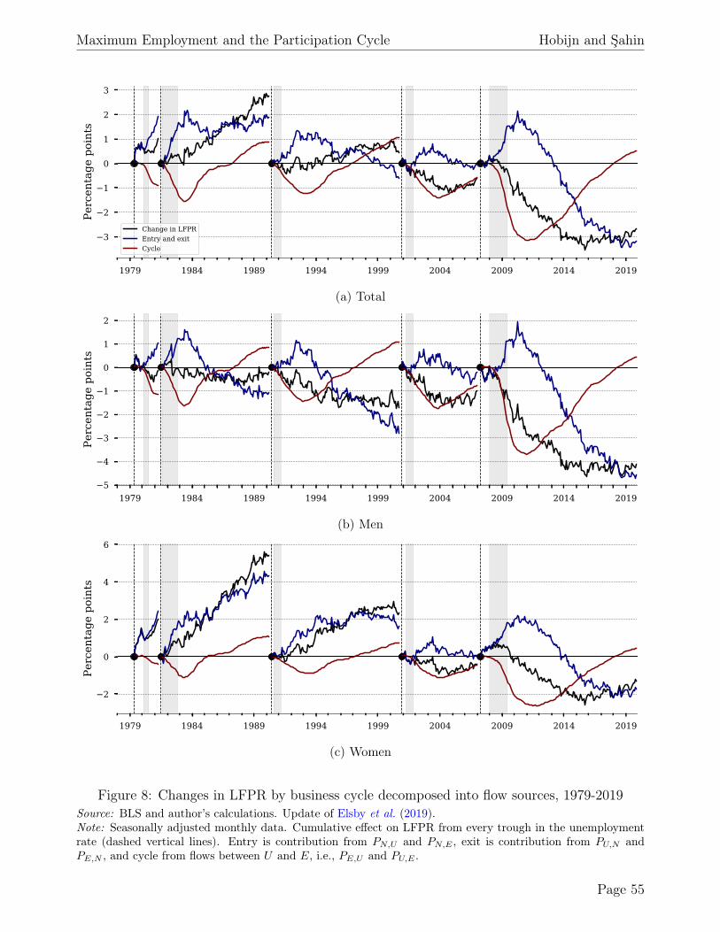
Maximum Employment and the Participation Cycle Hobijn and Şahin
1979 1984 1989 1994 1999 2004 2009 2014 2019
3
2
1
0
1
2
3Pe
rcen
tage
poi
nts
Change in LFPREntry and exitCycle
(a) Total
1979 1984 1989 1994 1999 2004 2009 2014 20195
4
3
2
1
0
1
2
Perc
enta
ge p
oint
s
(b) Men
1979 1984 1989 1994 1999 2004 2009 2014 2019
2
0
2
4
6
Perc
enta
ge p
oint
s
(c) Women
Figure 8: Changes in LFPR by business cycle decomposed into flow sources, 1979-2019Source: BLS and author’s calculations. Update of Elsby et al. (2019).Note: Seasonally adjusted monthly data. Cumulative effect on LFPR from every trough in the unemploymentrate (dashed vertical lines). Entry is contribution from PN,U and PN,E , exit is contribution from PU,N andPE,N , and cycle from flows between U and E, i.e., PE,U and PU,E .
Page 55

Maximum Employment and the Participation Cycle Hobijn and Şahin
1979 1984 1989 1994 1999 2004 2009 2014 2019
3
2
1
0
1
Perc
enta
ge p
oint
s
Unemployment cycleLFPR cycle
(a) Total
1979 1984 1989 1994 1999 2004 2009 2014 20195
4
3
2
1
0
1
Perc
enta
ge p
oint
s
(b) Men
1979 1984 1989 1994 1999 2004 2009 2014 2019
2
1
0
1
Perc
enta
ge p
oint
s
(c) Women
Figure 9: Cyclical pressures on EPOP ratio by cycle, 1979-2019Source: BLS, CBO, and author’s calculations.Note: Seasonally adjusted monthly data. Cumulative effect on EPOP ratio from every trough in the unem-ployment rate (dashed vertical lines). Unemployment gap is cumulative sum of −LFPRt∆ut and LFPR cycleis cumulative sum of (1− ut) ∆LFPRc
t . See equation (19). u∗t is the CBO’s natural rate of unemployment(long-term).
Page 56

Maximum Employment and the Participation Cycle Hobijn and Şahin
1979 1984 1989 1994 1999 2004 2009 2014 2019
14
16
18
20
22
Perc
enta
ge p
oint
Attachment wedge
(a) Total
1979 1984 1989 1994 1999 2004 2009 2014 2019
10
12
14
16
18
20
Perc
enta
ge p
oint
Attachment wedge
(b) Men
1979 1984 1989 1994 1999 2004 2009 2014 2019
18
20
22
24
26
Perc
enta
ge p
oint
Attachment wedge
(c) Women
Figure 10: Attachment wedge, total and by gender, 1978-2019Source: BLS and author’s calculations. Seasonally adjusted monthly data. Attachment wedge is differencebetween margin-adjusted pu,n,t and pe,n,t.
Page 57

Maximum Employment and the Participation Cycle Hobijn and Şahin
1979 1984 1989 1994 1999 2004 2009 2014 2019
2
0
2
4
6Pe
rcen
tage
poi
nts
TotalMenWomen
(a) Sex
1979 1984 1989 1994 1999 2004 2009 2014 2019
4
2
0
2
4
6
8
10
Perc
enta
ge p
oint
s
Total16-2425-5455 and over
(b) Age
1979 1984 1989 1994 1999 2004 2009 2014 2019
4
2
0
2
4
6
8
Perc
enta
ge p
oint
s
TotalLess than high schoolHigh school diplomaSome collegeCollege degree or higher
(c) Education
1979 1984 1989 1994 1999 2004 2009 2014 2019
4
2
0
2
4
6
8
Perc
enta
ge p
oint
s
TotalWhiteBlackHispanic
(d) Race and ethnicity
Figure 11: Change in unemployment rate across recessions by different demographics, 1978-2019Source: BLS and author’s calculations.
Page 58
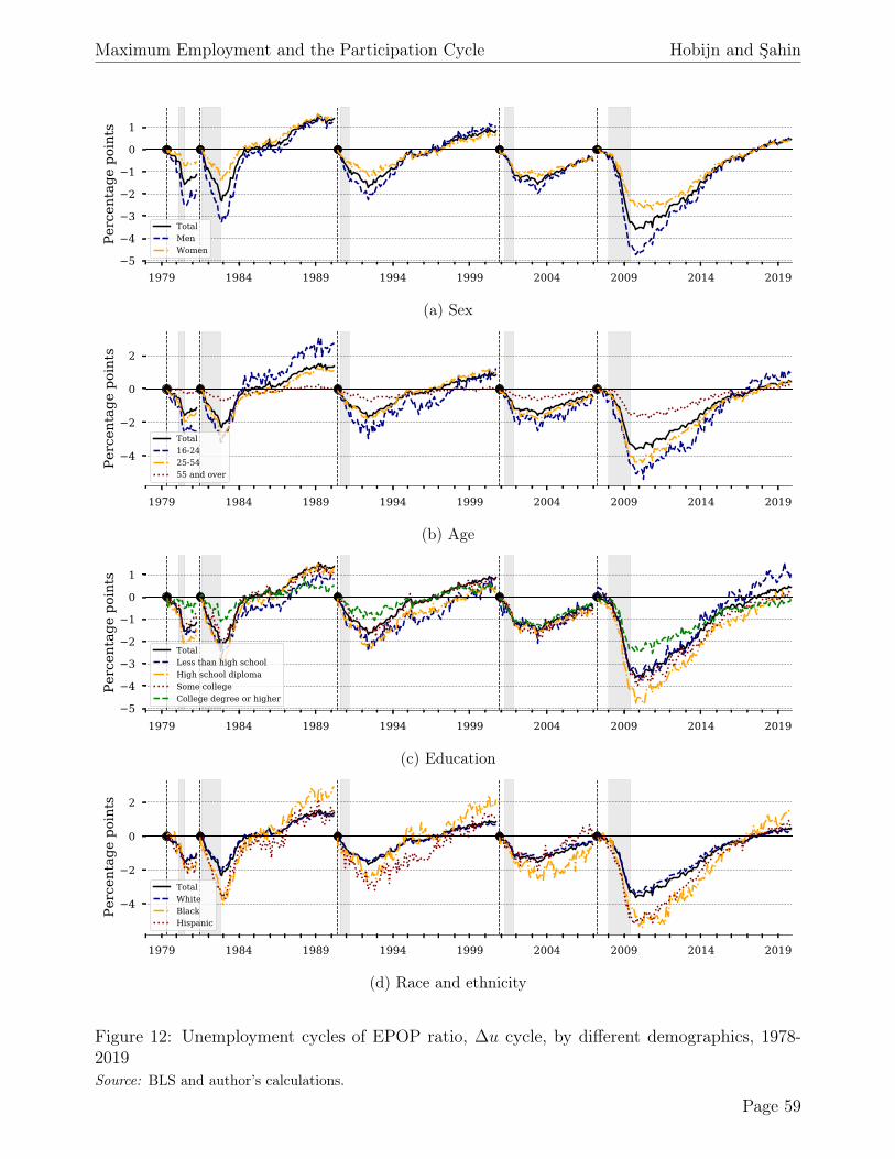
Maximum Employment and the Participation Cycle Hobijn and Şahin
1979 1984 1989 1994 1999 2004 2009 2014 20195
4
3
2
1
0
1Pe
rcen
tage
poi
nts
TotalMenWomen
(a) Sex
1979 1984 1989 1994 1999 2004 2009 2014 2019
4
2
0
2
Perc
enta
ge p
oint
s
Total16-2425-5455 and over
(b) Age
1979 1984 1989 1994 1999 2004 2009 2014 20195
4
3
2
1
0
1
Perc
enta
ge p
oint
s
TotalLess than high schoolHigh school diplomaSome collegeCollege degree or higher
(c) Education
1979 1984 1989 1994 1999 2004 2009 2014 2019
4
2
0
2
Perc
enta
ge p
oint
s
TotalWhiteBlackHispanic
(d) Race and ethnicity
Figure 12: Unemployment cycles of EPOP ratio, ∆u cycle, by different demographics, 1978-2019Source: BLS and author’s calculations.
Page 59

Maximum Employment and the Participation Cycle Hobijn and Şahin
1979 1984 1989 1994 1999 2004 2009 2014 2019
3
2
1
0
1Pe
rcen
tage
poi
nts
TotalMenWomen
(a) Sex
1979 1984 1989 1994 1999 2004 2009 2014 20193.02.52.01.51.00.50.00.51.0
Perc
enta
ge p
oint
s
Total16-2425-5455 and over
(b) Age
1979 1984 1989 1994 1999 2004 2009 2014 2019
3
2
1
0
1
Perc
enta
ge p
oint
s
TotalLess than high schoolHigh school diplomaSome collegeCollege degree or higher
(c) Education
1979 1984 1989 1994 1999 2004 2009 2014 2019
3
2
1
0
1
Perc
enta
ge p
oint
s
TotalWhiteBlackHispanic
(d) Race and ethnicity
Figure 13: Participation cycles of EPOP ratio, LFPRc, by different demographics, 1978-2019Source: BLS and author’s calculations.
Page 60
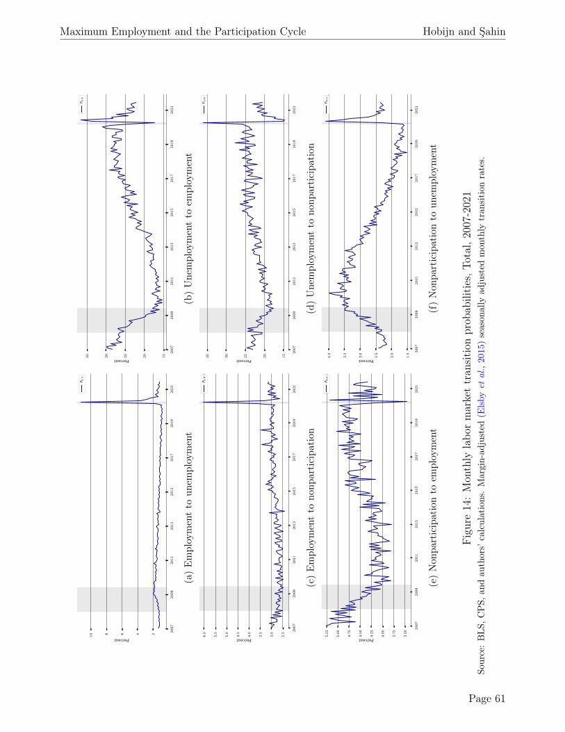
Maximum Employment and the Participation Cycle Hobijn and Şahin
2007
2009
2011
2013
2015
2017
2019
2021
246810 Percent
P E,U
(a)Employ
mentto
unem
ployment
2007
2009
2011
2013
2015
2017
2019
2021
1520253035 Percent
P U,E
(b)Une
mploy
mentto
employment
2007
2009
2011
2013
2015
2017
2019
2021
2.5
3.0
3.5
4.0
4.5
5.0
5.5
6.0
Percent
P E,N
(c)Employ
mentto
nonp
articipa
tion
2007
2009
2011
2013
2015
2017
2019
2021
1520253035 Percent
P U,N
(d)Une
mploy
mentto
nonp
articipa
tion
2007
2009
2011
2013
2015
2017
2019
2021
3.50
3.75
4.00
4.25
4.50
4.75
5.00
5.25
Percent
P N,E
(e)Non
participationto
employment
2007
2009
2011
2013
2015
2017
2019
2021
1.5
2.0
2.5
3.0
3.5
4.0
Percent
P N,U
(f)Non
participationto
unem
ployment
Figure14
:Mon
thly
labo
rmarkettran
sition
prob
abilities,T
otal,2
007-20
21So
urce:BLS
,CPS,
andau
thors’
calculations.Margin-ad
justed
(Elsby
etal
.,2015)season
ally
adjusted
mon
thly
tran
sition
rates.
Page 61

Maximum Employment and the Participation Cycle Hobijn and Şahin
2007 2009 2011 2013 2015 2017 2019 2021
2
3
4
5
6
7
8
9Pe
rcen
tActual UPOPFlow steady state UPOP
(a) unemployment-to-population (UPOP)
2007 2009 2011 2013 2015 2017 2019 2021
30
35
40
45
50
55
60
65
70
Perc
ent
Actual LFPRFlow steady state LFPR
(b) labor force participation rate (LFPR)
2007 2009 2011 2013 2015 2017 2019 2021
20
30
40
50
60
Perc
ent
Actual EPOPFlow steady state EPOP
(c) employment-to-population (EPOP)
Figure 15: Actual and flow steady-state UPOP ratio, EPOP ratio, LFPR, Jan 2007-Jun 2021Source: BLS, CPS, and authors’ calculations.
Page 62

Maximum Employment and the Participation Cycle Hobijn and Şahin
2007 2009 2011 2013 2015 2017 2019 2021
0
2
4
6
8
10
12Pe
rcen
tage
poi
nts
TotalMenWomen
(a) Sex
2007 2009 2011 2013 2015 2017 2019 2021
0
5
10
15
20
Perc
enta
ge p
oint
s
Total16-2425-5455 and over
(b) Age
2007 2009 2011 2013 2015 2017 2019 2021
5
0
5
10
15
Perc
enta
ge p
oint
s
TotalLess than high schoolHigh school diplomaSome collegeCollege degree or higher
(c) Education
2007 2009 2011 2013 2015 2017 2019 2021
2.5
0.0
2.5
5.0
7.5
10.0
12.5
15.0
Perc
enta
ge p
oint
s
TotalWhiteBlackHispanic
(d) Race and ethnicity
Figure 16: Change in unemployment rate across in Great and COVID-19 RecessionsSource: BLS and author’s calculations.
Page 63

Maximum Employment and the Participation Cycle Hobijn and Şahin
2007 2009 2011 2013 2015 2017 2019 2021
4
3
2
1
0
Perc
enta
ge p
oint
s
TotalMenWomen
(a) Sex
2007 2009 2011 2013 2015 2017 2019 2021
6
4
2
0
2
Perc
enta
ge p
oint
s
Total16-2425-5455 and over
(b) Age
2007 2009 2011 2013 2015 2017 2019 20217
6
5
4
3
2
1
0
Perc
enta
ge p
oint
s
TotalLess than high schoolHigh school diplomaSome collegeCollege degree or higher
(c) Education
2007 2009 2011 2013 2015 2017 2019 2021
4
3
2
1
0
Perc
enta
ge p
oint
s
TotalWhiteBlackHispanic
(d) Race and ethnicity
Figure 17: Change in participation rate in Great and COVID-19 RecessionsSource: BLS and author’s calculations.
Page 64

Maximum Employment and the Participation Cycle Hobijn and Şahin
2022 2023 2024 2025 2026
3.5
4.0
4.5
5.0
5.5
6.0
perc
ent
Post-2014 recoveryAccelerated post-2014 recovery
(a) Unemployment rate
2022 2023 2024 2025 2026
1.6
1.4
1.2
1.0
0.8
0.6
0.4
0.2
0.0
Perc
enta
ge p
oint
s
Post-2014 recovery: Unemployment cyclePost-2014 recovery: Participation cycleAccelerated post-2014 recovery: Unemployment cycleAccelerated post-2014 recovery: Participation cycle
(b) Unemployment and participation cycles
Figure 18: Projections based on post-2014 recovery in flow ratesSource: BLS and author’s calculations.Note: Unemployment and participation cycles plotted in terms of percentage point cyclical pressures on theEPOP ratio.“Post-2014 recovery” based on path of flow rates from Sep 2014 - Feb 2020. In case of “Acceleratedpost-2014 recovery”path of flow rates is three times faster than the baseline case. Transition probabilities forprojections calculated using equations (38)-(40) explained in the Appendix. These projections are not meantas forecasts but to illustrate the potential labor market dynamics during the recovery going forward.
Page 65

Maximum Employment and the Participation Cycle Hobijn and Şahin
Table1:
Uneveness
inun
employ
mentan
dpa
rticipationcycles.
u∆u
LFPR
Att.
wedge
∆ucycle
trou
ghLFPR
c
trou
ghTroug
hratio
LFPR
c
lag
topic
grou
p
Total
6.2
3.3
65.2
20.0
-2.2
-1.5
69.3
9.0
Sex
Men
6.3
3.9
74.0
17.5
-3.0
-1.8
59.9
8.4
Wom
en6.1
2.6
57.2
23.0
-1.5
-1.1
73.6
11.0
Age
16-24
12.7
5.2
63.0
23.2
-3.3
-1.2
35.5
4.0
25-54
5.1
3.2
82.2
17.2
-2.6
-1.5
56.7
8.2
55an
dover
3.9
2.4
34.5
20.7
-0.8
-0.7
81.5
13.8
Edu
cation
Less
than
high
scho
ol12.6
5.8
42.7
24.7
-2.5
-1.5
60.7
7.6
Highscho
oldiplom
a7.0
4.2
65.2
18.8
-2.8
-1.8
65.2
9.8
Somecollege
5.2
3.0
71.6
18.6
-2.2
-1.3
58.4
8.8
College
degree
orhigh
er2.8
1.7
79.0
15.3
-1.3
-0.8
49.7
2.2
Race
White
5.4
3.0
65.5
19.0
-2.0
-1.5
73.8
8.8
Black
11.8
5.4
63.2
22.5
-3.4
-1.6
45.2
5.2
Ethnicity
Hispa
nic
8.6
4.9
66.7
21.4
-3.3
-1.9
58.3
5.8
Sour
ce:BLS
,CPS,
andau
thors’
calculations
Not
es:Sa
mpleis
allrecessions,except
theCOVID
recession.
uis
theaverageun
employmentrate
from
1978-2019.LFPR
istheaveragepa
rticipation
rate.Att.wedge
isaveragefrom
1994-2019(due
toCPSredesign
).∆uis
averagepe
rcentage
pointincrease
inun
employ
mentrate
across
recessions
(exceptCOVID
recession).
∆u
cycletrou
ghis
averagetrou
ghin
EPOP
unem
ploymentcycleacross
recessions,LFPR
ctrou
ghis
thesameforthe
participationcycle.
Troug
hratiois
theaverageLFPR
ctrou
ghas
ape
rcentof
the
∆ucycleacross
recessions.LFPR
clagis
theaveragenu
mbe
rof
mon
thsthat
thepa
rticipationcycletrou
ghlags
theun
employmentcycleacross
recessions.
Page 66

Maximum Employment and the Participation Cycle Hobijn and Şahin
Table 2: Deviations from the Perry-Okun rule by group.
mean stdtopic group
Total 0.03 0.17Sex Men 0.00 0.24
Women 0.02 0.15Age 16-24 -0.22 0.39
25-54 -0.04 0.2055 and over 0.01 0.11
Education Less than high school -0.05 0.32High school diploma 0.04 0.25Some college -0.04 0.22College degree or higher -0.00 0.19
Race White 0.05 0.18Black -0.12 0.50
Ethnicity Hispanic -0.05 0.48
Source: BLS, CBO, CPS, and authors’ calculationsNotes: Mean and standard deviation of the residual from the Perry-Okun rule (in percentage points of EPOPratio). Perry-Okun rule is calculated as difference between cumulative 12-month change in participation cycleand unemployment cycle of EPOP during labor market expansions when the unemployment rate is less thanhalf a percentage point higher than the long-run natural rate of the CBO.
Page 67
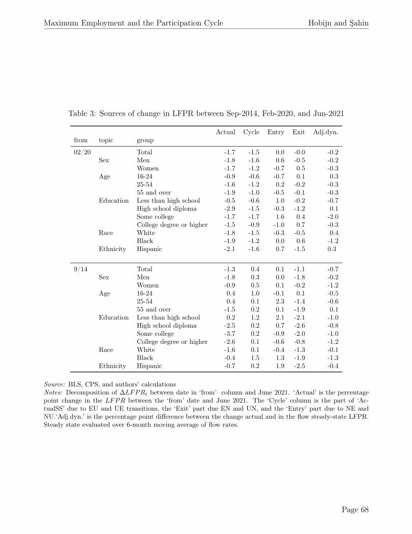
Maximum Employment and the Participation Cycle Hobijn and Şahin
Table 3: Sources of change in LFPR between Sep-2014, Feb-2020, and Jun-2021
Actual Cycle Entry Exit Adj.dyn.from topic group
02/20 Total -1.7 -1.5 0.0 -0.0 -0.2Sex Men -1.8 -1.6 0.6 -0.5 -0.2
Women -1.7 -1.2 -0.7 0.5 -0.3Age 16-24 -0.9 -0.6 -0.7 0.1 0.3
25-54 -1.6 -1.2 0.2 -0.2 -0.355 and over -1.9 -1.0 -0.5 -0.1 -0.3
Education Less than high school -0.5 -0.6 1.0 -0.2 -0.7High school diploma -2.9 -1.5 -0.3 -1.2 0.1Some college -1.7 -1.7 1.6 0.4 -2.0College degree or higher -1.5 -0.9 -1.0 0.7 -0.3
Race White -1.8 -1.5 -0.3 -0.5 0.4Black -1.9 -1.2 0.0 0.6 -1.2
Ethnicity Hispanic -2.1 -1.6 0.7 -1.5 0.3
9/14 Total -1.3 0.4 0.1 -1.1 -0.7Sex Men -1.8 0.3 0.0 -1.8 -0.2
Women -0.9 0.5 0.1 -0.2 -1.2Age 16-24 0.4 1.0 -0.1 0.1 -0.5
25-54 0.4 0.1 2.3 -1.4 -0.655 and over -1.5 0.2 0.1 -1.9 0.1
Education Less than high school 0.2 1.2 2.1 -2.1 -1.0High school diploma -2.5 0.2 0.7 -2.6 -0.8Some college -3.7 0.2 -0.9 -2.0 -1.0College degree or higher -2.6 0.1 -0.6 -0.8 -1.2
Race White -1.6 0.1 -0.4 -1.3 -0.1Black -0.4 1.5 1.3 -1.9 -1.3
Ethnicity Hispanic -0.7 0.2 1.9 -2.5 -0.4
Source: BLS, CPS, and authors’ calculationsNotes: Decomposition of ∆LFPRt between date in ‘from’ column and June 2021. ‘Actual’ is the percentagepoint change in the LFPR between the ‘from’ date and June 2021. The ‘Cycle’ column is the part of ‘Ac-tualSS’ due to EU and UE transitions, the ‘Exit’ part due EN and UN, and the ‘Entry’ part due to NE andNU.‘Adj.dyn.’ is the percentage point difference between the change actual and in the flow steady-state LFPR.Steady state evaluated over 6-month moving average of flow rates.
Page 68

Maximum Employment and the Participation Cycle Hobijn and Şahin
A Mathematical and computational details
Distributed Lag of Past Changes in Flow Steady State
Recursively solving (11) forward we obtain
∆st = P t (I + P t−1)P−1t−1∆st−1 − P t∆st (23)
= P t (I + P t−1) (I + P t−2)P t−2∆st−2 − P t (I + P t−1) ∆st−1 − P t∆st (24)
= −P t (I + P t)−1
∞∑l=0
l∏j=0
(I + P t−j) ∆st−l (25)
The minus sign in the last line of this equation might be confusing, but most elements of P t,
except the first row second column, are negative. Thus, the current change in the labor market
state vector is a complicated lag structure of the past changes in the flow steady-state.
Substituting in (14) yields
∆st = P t (I + P t)−1
∞∑l=0
l∏j=0
(I + P t−j)
[1
2(P t−l + P t−l−1)
]−1(26)
×[∆dt−l +
1
2∆P t−l (st−l + st−l−1)
]. (27)
Participation cycle and the attachment wedge
The LFPR cycle is the changes in ι′2st due changes in PE,U,t and PU,E,t. The main intuition of
what is driving this cycle is to ignore the lagged effects because of deviations from the steady
state and, instead, focus on the effect of PE,U,t and PU,E,t on ι′st.
This involves identifying the parts of (14) associated with ∆PE,U,t and ∆PU,E,t. For this, it
is important to realize that
∂dt∂PE,U,t
=∂dt
∂PU,E,t= 0,
∂P t
∂PE,U,t=
[−1 0
1 0
], and
∂P t
∂PU,E,t=
[0 1
0 −1
]. (28)
Using equation (14) this yields that
∂st∂PE,U,t
= (P t + P t−1)−1
[ (Et + Et−1
)−(Et + Et−1
)] and (29)
∂st∂Pu,e,t
= (P t + P t−1)−1
[−(Ut + Ut−1
)(Ut + Ut−1
) ] , (30)
Page 69

Maximum Employment and the Participation Cycle Hobijn and Şahin
The change in the LFPR cycle is given by
∆LFPRct = ι′2
(∂st
∂PE,U,t∆pE,U,t +
∂st∂PU,E,t
∆pU,E,t
)(31)
= ι′2 (P t + P t−1)−1
[1
−1
] ((Et + Et−1
)∆pe,u,t −
(Ut + Ut−1
)∆pU,E,t
)(32)
= ι′2 (P t + P t−1)−1
[1
−1
]LFPRt ((1− ut) ∆pe,u,t − ut∆pu,e,t) , (33)
where,
LFPRt = 1/2(Et + Et−1 + Ut + Ut−1
)and ut =
1/2(Ut + Ut−1
)LFPRt
. (34)
LFPRt is the flow steady-state labor force participation rate and ut is the flow steady-state
unemployment rate, both averaged across periods t and t−1. Solving for the matrix expression
at the beginning of this equation yields
ι′2P−1t
[1
−1
]=
1
Dt
(PE,N,t − PU,N,t
)(35)
Where Dt is the determinant of P t = 1/2 (P t + P t−1), PE,N,t = 1/2 (PE,N,t + PE,N,t−1), and
PU,N,t = 1/2 (PU,N,t + PU,N,t−1).
This gives that the part of the change in the LFPR cycle that works through the contem-
poraneous effect on the flow steady state equals
∆LFPRct = − 1
Dt
LFPRt
(PU,N,t − PE,N,t
)((1− ut) ∆PE,U,t − ut∆PU,E,t) (36)
Perry-Okun rule residuals
The mean of the Perry-Okun residual for group i, µi, reported in Table 2, is calculated as
µi =1
nH
∑t∈H
εi,t, εi,t =
12∑j=0
(1− ui,t−j) ∆LFPRci,t−j︸ ︷︷ ︸
participation cycle
− 12∑j=0
−LFPRi,t−j∆ui,t−j︸ ︷︷ ︸unemployment cycle
, (37)
Here H is the set of months, t that occur in a hot labor market that has lasted for more than a
year. This consists of months t during labor market expansions when the unemployment rate,
ut, is smaller than the natural rate, u∗t , plus 0.5 percentage points and the same is true for
t − 12. nH is the number of months in this set. The standard deviations are calculated in a
Page 70

Maximum Employment and the Participation Cycle Hobijn and Şahin
similar way.
Path of transition probabilities for projections
The assumed paths of the transition probabilities for the projections presented in Subsection
6.4 are calculated using
PS,S′,t = φδt (PS,S′,Jun−21 − PS,S′,Sep−14) + PS,S′,τ , where (38)
τ = min {Sep− 14 + δ ×m (t, Jun− 21) , Feb− 2020} , and (39)
φ = m (t, Jun− 21) /m (t, Jun− 21) (40)
Here m (t′, t) measures the distance between two dates in months. The parameter δ determines
the speed of the recovery in the projections. For the baseline case, labeled the “Post-2014
recovery”, δ = 1. For the accelerated recovery case δ = 3.
B Data details
Reason for nonparticipation
The reason for nonparticipation is constructed by combining data on an individuals’ employ-
ment status, reason for not looking for work, and major activity while not in the labor force.
Retired persons are the nonparticipants who report their employment status as retired. For
those who are not retired, we first classify non-participants based on the reasons they report
for not looking for work. Those who do not report such a reason are then classified based on
their main activity while not participating in the labor market. 45
C Additional empirical results
45The results in this paper are calculated using the CPS-IPUMS extracts described in Flood et al. (2020).
Page 71

Maximum Employment and the Participation Cycle Hobijn and Şahin
2004 2009 2014 2019 2024 2029
32
34
36
38
40
42
44pe
rcen
t
Actual
(a) Total, 65 and over
2004 2009 2014 2019 2024 2029
87
88
89
90
91
92
perc
ent
Actual
(b) Men, prime age (25-54)
2004 2009 2014 2019 2024 2029
52
54
56
58
60
62
64
66
perc
ent
Actual
(c) Women, 55 to 64
Figure C.1: BLS LFPR projections for different age-gender groups.Source: BLS Labor Force Projections, CPS, and authors’ calculations.Notes: Vintage of forecast is indicated by dot. Actual is seasonally adjusted monthly observations. Forecastsare linearly interpolated between beginning and end of 10-year forecast period.
Page 72

Maximum Employment and the Participation Cycle Hobijn and Şahin
1979
1984
1989
1994
1999
2004
2009
2014
2019
0.75
1.00
1.25
1.50
1.75
2.00
2.25
2.50
2.75
Percent
P E,U
(a)Employ
mentto
unem
ployment
1979
1984
1989
1994
1999
2004
2009
2014
2019
1520253035 Percent
P U,E
(b)Une
mploy
mentto
employment
1979
1984
1989
1994
1999
2004
2009
2014
2019
1.8
2.0
2.2
2.4
2.6
2.8
Percent
P E,N
(c)Employ
mentto
nonp
articipa
tion
1979
1984
1989
1994
1999
2004
2009
2014
2019
1.8
2.0
2.2
2.4
2.6
2.8
Percent
P E,N
(d)Une
mploy
mentto
nonp
articipa
tion
1979
1984
1989
1994
1999
2004
2009
2014
2019
4.0
4.5
5.0
5.5
6.0
6.5
7.0
7.5
8.0
Percent
P N,E
(e)Non
participationto
employment
1979
1984
1989
1994
1999
2004
2009
2014
2019
2.0
2.5
3.0
3.5
4.0
4.5
5.0
Percent
P N,U
(f)Non
participationto
unem
ployment
FigureC.2:Mon
thly
labo
rmarkettran
sition
prob
abilities,M
en,1
978-20
19So
urce:BLS
,CPS,
andau
thors’
calculations.Margin-ad
justed
(Elsby
etal
.,2015)season
ally
adjusted
mon
thly
tran
sition
rates.
Page 73

Maximum Employment and the Participation Cycle Hobijn and Şahin
1979
1984
1989
1994
1999
2004
2009
2014
2019
0.8
1.0
1.2
1.4
1.6
1.8
2.0
2.2
Percent
P E,U
(a)Employ
mentto
unem
ployment
1979
1984
1989
1994
1999
2004
2009
2014
2019
1520253035 Percent
P U,E
(b)Une
mploy
mentto
employment
1979
1984
1989
1994
1999
2004
2009
2014
2019
3.0
3.5
4.0
4.5
5.0
5.5
Percent
P E,N
(c)Employ
mentto
nonp
articipa
tion
1979
1984
1989
1994
1999
2004
2009
2014
2019
3.0
3.5
4.0
4.5
5.0
5.5
Percent
P E,N
(d)Une
mploy
mentto
nonp
articipa
tion
1979
1984
1989
1994
1999
2004
2009
2014
2019
3.5
4.0
4.5
5.0
5.5
Percent
P N,E
(e)Non
participationto
employment
1979
1984
1989
1994
1999
2004
2009
2014
2019
1.5
2.0
2.5
3.0
3.5
Percent
P N,U
(f)Non
participationto
unem
ployment
FigureC.3:Mon
thly
labo
rmarkettran
sition
prob
abilities,W
omen,1
978-20
19So
urce:BLS
,CPS,
andau
thors’
calculations.Margin-ad
justed
(Elsby
etal
.,2015)season
ally
adjusted
mon
thly
tran
sition
rates.
Page 74

Maximum Employment and the Participation Cycle Hobijn and Şahin
1979
1984
1989
1994
1999
2004
2009
2014
2019
42024
Percentage point
Cha
nge
in L
FPR
Initi
al c
hang
e in
EPO
PIn
itial
cha
nge
in U
POP
pEU
pEN
pUE
pUN
pNE
pNU
Initi
al s
tate
FigureC.4:Six-flo
wdecompo
sition
ofchan
gein
LFPR.
Sour
ce:BLS
,CPS,
andau
thor’s
calculations
Not
e:Cum
ulativecontribu
tion
sof
chan
gesin
each
ofthesixlabo
rmarketstatus
flow
rateson
thechan
gein
theEPOP
ratiosincethebe
ginn
ingof
1978.
Page 75

Maximum Employment and the Participation Cycle Hobijn and Şahin
1979 1984 1989 1994 1999 2004 2009 2014 2019
4
2
0
2
4
Perc
enta
ge p
oint
Change in LFPRExitEntryCycleInitial state
(a) Total
1979 1984 1989 1994 1999 2004 2009 2014 2019
12
10
8
6
4
2
0
2
Perc
enta
ge p
oint
Change in LFPRExitEntryCycleInitial state
(b) Men
1979 1984 1989 1994 1999 2004 2009 2014 2019
2
0
2
4
6
8
10
Perc
enta
ge p
oint
Change in LFPRExitEntryCycleInitial state
(c) Women
Figure C.5: Change in LFPR since January 1978 decomposed, 1978-2019Source: BLS and author’s calculations. Update of Elsby et al. (2019).Note: Seasonally adjusted monthly data. Cumulative effect on EPOP ratiosince January 1978. Entry iscontribution from PN,U and PN,E , exit is contribution from PU,N and PE,N , and cycle from flows between Uand E, i.e., PE,U and PU,E .
Page 76

Maximum Employment and the Participation Cycle Hobijn and Şahin
2007 2009 2011 2013 2015 2017 2019 2021
2
3
4
5
6
7
8
9Pe
rcen
tActual UPOPFlow steady state UPOP
(a) Total
2007 2009 2011 2013 2015 2017 2019 2021
3
4
5
6
7
8
9
Perc
ent
Actual UPOPFlow steady state UPOP
(b) Men
2007 2009 2011 2013 2015 2017 2019 2021
2
3
4
5
6
7
8
9
Perc
ent
Actual UPOPFlow steady state UPOP
(c) Women
Figure C.6: Actual and flow steady-state UPOP ratio, Jan 2007-Jun 2021Source: BLS, CPS, and authors’ calculations.
Page 77

Maximum Employment and the Participation Cycle Hobijn and Şahin
Table C.4: Sources of change in UPOP between Sep-2014, Feb-2020, and Jun-2021
Actual Cycle Entry Exit Adj.dyn.from topic group
02/20 Total 1.5 0.7 0.5 0.2 0.1Sex Men 1.7 0.9 0.5 0.2 0.1
Women 1.3 0.5 0.5 0.2 0.1Age 16-24 1.3 0.6 0.4 0.2 0.1
25-54 1.9 1.0 0.6 0.2 0.155 and over 0.8 0.3 0.3 0.1 0.1
Education Less than high school 0.9 0.3 0.2 0.3 0.0High school diploma 1.5 0.7 0.5 0.1 0.2Some college 1.8 0.9 0.7 0.1 0.2College degree or higher 1.2 0.5 0.4 0.2 0.1
Race White 1.3 0.7 0.4 0.2 0.1Black 1.9 0.7 0.8 0.1 0.2
Ethnicity Hispanic 2.2 1.1 0.6 0.3 0.3
9/14 Total -0.1 -0.2 -0.2 0.2 0.0Sex Men -0.1 -0.1 -0.3 0.3 -0.0
Women -0.1 -0.2 -0.2 0.2 0.0Age 16-24 -1.5 -0.9 -1.2 0.5 0.1
25-54 0.2 -0.1 0.1 0.2 0.055 and over 0.1 -0.1 0.1 0.0 0.1
Education Less than high school -1.0 -0.6 -0.6 0.2 0.0High school diploma -0.2 -0.1 -0.2 0.1 0.1Some college -0.1 -0.1 -0.3 0.2 0.1College degree or higher 0.3 -0.0 0.1 0.1 0.1
Race White -0.0 -0.1 -0.2 0.2 0.0Black -1.3 -0.9 -0.7 0.2 0.0
Ethnicity Hispanic 0.1 -0.1 -0.3 0.4 0.2
Source: BLS, CPS, and authors’ calculationsNotes: Decomposition of ∆UPOPt between date in ‘from’ column and June 2021. ‘Actual’ is the percentagepoint change in the UPOP between the ‘from’ date and June 2021. The ‘Cycle’ column is the part of ‘Ac-tualSS’ due to EU and UE transitions, the ‘Exit’ part due EN and UN, and the ‘Entry’ part due to NE andNU.‘Adj.dyn.’ is the percentage point difference between the change actual and in the flow steady-state UPOP.Steady state evaluated over 6-month moving average of flow rates.
Page 78