maximizing power to track alzheimer's disease and mci

UNCO

RRECTED P

RO

OF

1 Maximizing power to track Alzheimer's disease and MCI progression by LDA-based2 weighting of longitudinal ventricular surface features

3 Boris A.Q1 Gutman a, Xue Hua a, Priya Rajagopalan a, Yi-Yu Chou a, Yalin Wang b, Igor Yanovsky c,4 Arthur W. Toga a, Clifford R. Jack Jr. d, Michael W. Weiner e,f,g, Paul M. Thompson a,h,⁎5 and for the Alzheimer's Disease Neuroimaging Initiative 1

6 a Imaging Genetics Center, Laboratory of Neuro Imaging, Dept. of Neurology, UCLA School of Medicine, Los Angeles, CA, USAQ117 b School of Computing, Informatics, and Decision Systems Engineering, Arizona State University, Tempe, AZ, USA8 c UCLA Joint Institute for Regional Earth System Science and Engineering, Los Angeles, CA, USA9 d Mayo Clinic, Rochester, MN, USA10 e Dept. of Radiology and Biomedical Imaging, UC San Francisco, San Francisco, CA, USA11 f Dept. of Medicine, UC San Francisco, San Francisco, CA, USA12 g Dept. of Psychiatry, UC San Francisco, San Francisco, CA, USA13 h Dept. of Psychiatry, Semel Institute, UCLA School of Medicine, Los Angeles, CA, USA

14

15

a b s t r a c ta r t i c l e i n f o

16 Article history:17 Accepted 18 December 201218 Available online xxxx19202122 Keywords:23 Linear Discriminant Analysis24 Shape analysis25 ADNI26 Lateral ventricles27 Alzheimer's disease28 Mild cognitive impairment29 Biomarker30 Drug trial31 Machine learning

32Wepropose a newmethod tomaximize biomarker efficiency for detecting anatomical change over time in serial33MRI. Drug trials using neuroimaging become prohibitively costly if vast numbers of subjects must be assessed, so34it is vital to develop efficient measures of brain change. A popular measure of efficiency is the minimal sample35size (n80) needed to detect 25% change in a biomarker, with 95% confidence and 80% power. For multivariate36measures of brain change, we can directly optimize n80 based on a Linear Discriminant Analysis (LDA). Here37we use a supervised learning framework to optimize n80, offering two alternative solutions. With a newmedial38surface modeling method, we track 3D dynamic changes in the lateral ventricles in 2065 ADNI scans. We apply39our LDA-based weighting to the results. Our best average n80—in two-fold nested cross-validation—is 104 MCI40subjects (95% CI: [94,139]) for a 1-year drug trial, and 75 AD subjects [64,102]. This compares favorably with41other MRI analysis methods. The standard “statistical ROI” approach applied to the same ventricular surfaces42requires165 MCI or 94 AD subjects. At 2 years, the best LDA measure needs only 67 MCI and 52 AD subjects,43versus 119 MCI and 80 AD subjects for the stat-ROI method. Our surface-based measures are unbiased: they44give no artifactual additive atrophy over three time points. Our results suggest that statistical weighting may45boost efficiency of drug trials that use brain maps.46© 2012 Published by Elsevier Inc.

4748

49

50

51 Introduction

52 Biomarkers of Alzheimer's disease based on brain imaging must53 offer relatively high power to detect longitudinal changes in subjects54 scanned repeatedly over time (Cummings, 2010; Ross et al., 2012;55 WymanQ12 et al., accepted for publication). Even so, recruitment and56 scanning are costly, and a drug trial may not be attempted at all,

57unless disease-slowing effects can be detected in an achievable sam-58ple size, and in a reasonable amount of time. Imaging measures from59standard structural MRI show considerable promise. Their use stems60from the premise that longitudinal changes may be more precisely61and reproducibly measured with MRI than comparable changes in62clinical, CSF, or proteomic assessments; clearly, whether that is true63depends on the measures used. Brain measures that are helpful for64diagnosis, such as PET scanning to assess brain amyloid or CSF mea-65sures of amyloid and tau proteins, may not be stable for longitudinal66trials that aim to slow disease progression. As a result, there is inter-67est in testing the reproducibility of biomarkers, as well as methods to68weight or combine them to make the most of all the available mea-69sures (Yuan et al., 2012).70Recent studies have tested the reproducibility and accuracy of a71variety of MRI-derived measures of brain change. Several are highly72correlated with clinical measures, and can predict future decline on73their own, or in combination with other relevantmeasures. Although74not the only important consideration, some analyses have assessed

NeuroImage xxx (2013) xxx–xxx

⁎ Corresponding author at: Imaging Genetics Center, Laboratory of Neuro Imaging,Dept. of Neurology, UCLA School of Medicine, Neuroscience Research Building 225E,635 Charles Young Drive, Los Angeles, CA 90095-1769, USA. Fax: +1 310 206 5518.

E-mail address: [email protected] (P.M. Thompson).1 Data used in preparation of this article were obtained from the Alzheimer's Disease

Neuroimaging Initiative (ADNI) database (adni.loni.ucla.edu). As such, the investiga-tors within the ADNI contributed to the design and implementation of ADNI and/orprovided data but did not participate in analysis or writing of this report. A completelisting of ADNI investigators can be found at: http://adni.loni.ucla.edu/wp-content/uploads/how_to_apply/ADNI_Acknowledgement_List.pdf.

YNIMG-10054; No. of pages: 16; 4C: 4, 5, 6, 7, 8, 9, 11, 14

1053-8119/$ – see front matter © 2012 Published by Elsevier Inc.http://dx.doi.org/10.1016/j.neuroimage.2012.12.052

Contents lists available at SciVerse ScienceDirect

NeuroImage

j ourna l homepage: www.e lsev ie r .com/ locate /yn img

Please cite this article as: Gutman, B.A., et al., Maximizing power to track Alzheimer's disease and MCI progression by LDA-based weighting oflongitudinal ventricular surface features, NeuroImage (2013), http://dx.doi.org/10.1016/j.neuroimage.2012.12.052

B X P Y Y IA C M P O

UNCO

RRECTED P

RO

OF

75 which MRI-based measures show greatest effect sizes for measuring76 brain change over time, while avoiding issues of bias and asymmetry77 that can complicate longitudinal image analysis (Fox et al., 2011;78 Holland et al., 2011; Hua et al., 2011), and while avoiding removing79 scans from the analysis that may lead to unfairly optimistic sample80 size estimates (Hua et al., 2012; Wyman et al., accepted for publication).81 Promising MRI-based measures include the brain boundary shift integral82 (Leung et al., 2012; Schott et al., 2010), the ventricular boundary shift83 integral (Schott et al., 2010) and measures derived from anatomical84 segmentation software such as Quarc or FreeSurfer, some of which have85 been recently modified to handle longitudinal data more accurately86 (Fischl and Dale, 2000; Holland and Dale, 2011; Reuter et al., 2012;87 Smith et al., 2002).88 Although several approaches are possible, one type of power analysis,89 advocated by the ADNI Biostatistics Core (Beckett, 2000), is to estimate90 theminimal sample size required to detect,with 80% power, a 25% reduc-91 tion in the mean annual change, using a two-sided test and standard92 significance level α=0.05 for a hypothetical two-arm study (treatment93 versus placebo). The estimate for the minimum sample size is computed94 from the formula below. β̂ denotes the annual change (average across the95 group) and σ̂ 2

D refers to the variance of the annual rate of change.

n ¼2σ̂ 2

D z1−α=2 þ zpower

� �2

0:25β̂� �2 ð1Þ

969798 Here zα is the value of the standard normal distribution for which P99 [Zbzα]=α. The sample size required to achieve 80% power is common-100 ly denoted by n80. Typical n80s for competitivemethods are under 150101 AD subjects and under 300 MCI subjects; the larger numbers for MCI102 reflect the fact that brain changes tend to be slower in MCI than AD103 and MCI is an etiologically more heterogeneous clinical category. For104 this reason, it is harder to detect a modification of changes that are105 inherently smaller, so greater sample sizes are needed to guarantee106 sufficient power to detect the slowing of disease. In addition, there is107 some interest in prevention trials targeting cognitively normal subjects108 who are at risk for AD by virtue of a family history or specific genetic109 profile (e.g., ApoE genotype); for these and other cohorts, efficiency110 must be a high priority, and measures that can distinguish AD from111 normal aging may be unable to track subtle changes efficiently in112 controls.113 Many algorithms can detect localized or diffuse changes in the brain,114 creating detailed 3D maps of changes (Avants et al., 2008; Leow et al.,115 2007; Shi et al., 2009), but the detail in the maps they produce is often116 disregarded when making sample size estimates according to Eq.117 (1), as the formula expects a single, univariate measure of change. In118 other words, it requires a single number, or ‘numeric summary’ to repre-119 sent all the relevant changes occurring within the brain. To mitigate this120 problem, Hua et al. (2009) defined a “statistical ROI” based on a small121 sample of AD subjects by thresholding the t-statistic of each feature122 (voxel) and summing the relevant features over the ROI; this approach123 was initially advocated in the FDG-PET literature to home in on regions124 that show greatest effects (Chen et al., 2010). In spirit, the statistical125 ROI is a rudimentary supervised learning approach, as it finds regions126 that show detectable effects in a training sample, and uses them to127 empower the analysis of future samples; the samples used are non-128 overlapping and independent, to avoid circularity. However, a simple129 threshold-based masking is known to potentially eliminate useful fea-130 tures, as binarization loses a lot of the information present in continuous131 weights (Duda et al., 2001). While many studies have used machine132 learning to predict the progression of neurodegenerative diseases and133 differentiate diagnostic groups such as AD, MCI, and controls (Kloppel134 et al., 2012; Kohannim et al., 2010; Vemuri et al., 2008), we found no135 attempts in the literature that used learning to directly optimize power136 to detect brain change. The closest work is perhaps that of Hobbs et al.

137(2010). In this paper, SVM was used to separate subjects with138Huntington's disease fromcontrols, and the resulting score used to calcu-139late sample size estimates. Our goal here was to generalize the very140simple binary feature weighting in the stat-ROI approach by directly141maximizing the power estimate in a training sample. A linear weighting142that optimizes Eq. (1) directly, while using multiple features at once,143is exactly analogous to a one-class Linear Discriminant Analysis (LDA),144discriminating the disease class from an imaginary sample of zero145mean whose covariance is identical to the disease group. We propose146two approaches to perform this task: one optimizes Eq. (1) directly by147Tikhonov regularization; the other is based on principal components148analysis (PCA).149A common criticism of the power analysis provided by Eq. (1) is150that it does not take into consideration normal ageing in non-high151risk healthy subjects (Holland et al., 2011). To mitigate this, several152researchers have proposed simply subtracting the mean value of153the change computed from controls, while using only the diseased154subjects for a variance estimate. This same issue can be directly155addressed in the LDA framework. In this case, the problem reduces156to the usual 2-class LDA classification, except that the covariance157structure is based on the diseased group only, and no assumption158of homoscedasticity (equality of variance) is made. This modification159is particularly useful for revealing subtle disease-specific atrophy in160regions that also change, to some extent, with normal aging.161We apply our LDA approach to maps of surface-based “thickness”162changes in the lateral ventricles over intervals of 1 and 2 years after a163baseline scan. The analyses are performed on MRI scans from the164ADNI-1 dataset. Using two follow-up time points, where available,165in addition to the baseline scan allows us to estimate the presence166of any longitudinal bias, or intransitivity, which has been a subject167of controversy in recent ADNI studies (Hua et al., 2011, 2012;168Thompson and Holland, 2011). To register the ventricles and compute169radial thickness measures, wemodify a recently proposed (Gutman et170al., 2012) medial curve algorithm for longitudinal registration. Our171general approach is to compute a single continuous curve skeleton172and use the curve to induce feature functions on the surface. Shape173registration is then performed parametrically by minimizing the L2

174difference (summed squared difference) between corresponding fea-175ture functions of a pair of shapes.176We note that ventricular expansion is not specific to AD and the177ventricles are often also abnormally enlarged in vascular dementia,178frontotemporal lobar degeneration, traumatic brain injury, Huntington's179disease, and schizophrenia, among other conditions. Even so, using180detailed surface-basedmaps of the location of expansion—in conjunction181with amodified2-class LDA—helps to reveal aspects of ventricular expan-182sion associated with the progression of Alzheimer's disease.

183Materials and methods

184Alzheimer's Disease Neuroimaging Initiative

185Data used in the preparation of this article were obtained from186the Alzheimer's Disease Neuroimaging Initiative (ADNI) database187(adni.loni.ucla.edu). The ADNI was launched in 2003 by the National188Institute on Aging (NIA), the National Institute of Biomedical Imaging189and Bioengineering (NIBIB), the Food and Drug Administration (FDA),190private pharmaceutical companies and non-profit organizations, as191a $60 million, 5-year public-private partnership. The primary goal192of ADNI has been to test whether serial magnetic resonance imaging193(MRI), positron emission tomography (PET), other biological markers,194and clinical and neuropsychological assessment can be combined to195measure the progression of mild cognitive impairment (MCI) and196early Alzheimer's disease (AD). Determination of sensitive and specific197markers of very early AD progression is intended to aid researchers198and clinicians to develop new treatments and monitor their effective-199ness, as well as lessen the time and cost of clinical trials.

2 B.A. Gutman et al. / NeuroImage xxx (2013) xxx–xxx


(

A

UNCO

RRECTED P

RO

OF

200 The Principal Investigator of this initiative is Michael W. Weiner,201 MD, VA Medical Center and University of California, San Francisco.202 ADNI is the result of efforts of many co-investigators from a broad203 range of academic institutions and private corporations, and subjects204 have been recruited from over 50 sites across the U.S. and Canada. The205 initial goal of ADNI was to recruit 800 adults, ages 55 to 90, to participate206 in the research, approximately 200 cognitively normal older individuals207 to be followed for 3 years, 400 people with MCI to be followed for208 3 years and 200 people with early AD to be followed for 2 years. For209 up-to-date information, see www.adni-info.org.210 Longitudinal brain MRI scans (1.5 T) and associated study data211 (age, sex, diagnosis, genotype, and family history of Alzheimer's dis-212 ease) were downloaded from the ADNI public database (http://213 www.loni.ucla.edu/ADNI/Data/) on July 1st 2012. The first phase of214 ADNI, i.e., ADNI-1, was a five-year study launched in 2004 to develop215 longitudinal outcome measures of Alzheimer's progression using216 serial MRI, PET, biochemical changes in CSF, blood and urine, and217 cognitive and neuropsychological assessments acquired at multiple218 sites similar to typical clinical trials.219 All subjects underwent thorough clinical and cognitive assess-220 ment at the time of scan acquisition. All AD patients met NINCDS/221 ADRDA criteria for probable AD (McKhann et al., 1984). The ADNI222 protocol lists more detailed inclusion and exclusion criteria (Mueller223 et al., 2005a, 2005b), available online http://www.alzheimers.org/224 clinicaltrials/fullrec.asp?PrimaryKey=208). The study was conducted225 according to the Good Clinical Practice guidelines, the Declaration of226 Helsinki and U.S. 21 CFR Part 50-Protection of Human Subjects, and227 Part 56-Institutional Review Boards. Written informed consent was228 obtained from all participants before performing experimental proce-229 dures, including cognitive testing.

230 MRI acquisition and image correction

231 All subjects were scanned with a standardized MRI protocol devel-232 oped for ADNI (Jack et al., 2008). Briefly, high-resolution structural233 brain MRI scans were acquired at 59 ADNI sites using 1.5 Tesla MRI234 scanners (GE Healthcare, PhilipsMedical Systems, or Siemens). Addition-235 al datawas collected at 3-T, but is not usedhere as itwas only collected on236 a subsample that is too small for making comparative assessments of237 power. Using a sagittal 3D MP-RAGE scanning protocol, the typical238 acquisition parameters were repetition time (TR) of 2400 ms, minimum239 full echo time (TE), inversion time (TI) of 1000 ms, flip angle of 8°,240 24 cm field of view, 192×192×166 acquisition matrix in the x-, y-,241 and z-dimensions, yielding a voxel size of 1.25×1.25×1.2 mm3, later242 reconstructed to 1 mm isotropic voxels. For every ADNI exam, the243 sagittal MP-RAGE sequence was acquired a second time, immediately244 after the first using an identical protocol. The MP-RAGE was run twice245 to improve the chance that at least one scan would be usable for analy-246 sis and for signal averaging if desired.247 The scan quality was evaluated by the ADNI MRI quality control248 (QC) center at theMayoClinic to exclude failed scans due tomotion, tech-249 nical problems, significant clinical abnormalities (e.g., hemispheric infarc-250 tion), or changes in scanner vendor during the time-series (e.g., from GE251 to Philips). Image corrections were applied using a standard processing252 pipeline consisting of four steps: (1) correction of geometric distortion253 due to gradient non-linearity (Jovicich et al., 2006), i.e. “gradwarp”254 (2) “B1-correction” for adjustment of image intensity inhomogeneity255 due to B1 non-uniformity (Jack et al., 2008), (3) “N3” bias field correc-256 tion for reducing residual intensity inhomogeneity (Sled et al., 1998),257 and (4) phantom-based geometrical scaling to remove scanner and258 session specific calibration errors (Gunter et al., 2006).

259 The ADNI-1 dataset

260 For our experiments, we analyzed data from 683 ADNI subjects261 with baseline and 1 year scans, and 542 subjects with baseline,

2621 year and 2 year scans. The former group consisted of 144 AD subjects263(age at screening: 75.5±7.4, 67 females (F)/77 males (M)), 337 subjects264with Mild Cognitive Impairment (MCI) (74.9±7.2, 122 F/215 M), and265202 age-matched healthy controls (NC) (76.0±5.1, 95 F/107 M). The2662-year group (i.e., people with scans at baseline, and after a 1-year and2672-year interval) had 111 AD (75.7±7.3, 52 F/59 M), 253 MCI (74.9±2687.1, 87 F/166 M), and 178 NC (76.2±5.2, 85 F/93 M) subjects. All raw269scans, images with different steps of corrections, and the standard270ADNI-1 collections are available to the general scientific community at271http://www.loni.ucla.edu/ADNI/Data/. We used exactly all ADNI sub-272jects available to us (on Feb. 1, 2012) who had both baseline and27312 month scans, and all subjects with 24 month scans (available274July 1, 2012). The use of all subjects without data exclusion has275been advocated by (Wyman et al., accepted for publication) and276(Hua et al., 2012), because any scan exclusion can lead to power277estimates that are unfairly optimistic, and many drug trials prohibit278the exclusion of any scans at all.

279Surface extraction

280Our surfaceswere extracted from9-parameter affine-registered, fully281processed T1-weighted anatomical scans. We used amodified version of282Chou's registration-based segmentation (Chou et al., 2008), using283inverse-consistent fluid registration with a mutual information fidelity284term (Leow et al., 2007). To avoid issues of bias and non-transitivity,285we segmented each of our subjects' two or three scans separately. In286this approach, a set of hand-labeled “templates” are aligned to each287scan, with multiple atlases being used to greatly reduce error. There288were an equal number of templates from each of the three diagnostic289groups, with an equal number of males and females in each. However,290using only AD or MCI templates instead is unlikely to have any measur-291able effect on the segmentation, due to the fact that many templates are292used (Table 1 Q13).

293Medial curve-based surface registration

294In this study, we focus onmapping changes in the lateral ventricles, a295fluid-filled space that expands as brain atrophy progresses (Fig. 1). Clear-296ly, other features could be used with our multivariate approach, and it297would be equally possible to apply the learning of discriminative features298from voxel-basedmaps of changes throughout the brain, as measured by299tensor-based morphometry, for example. The method is completely300general, and it could even be simultaneously applied to multiple types301of features; for example, thickness measures from anatomical surfaces302(cortical and subcortical), maps of volumetric changes throughout the303brain, and any other biomarkers such as maps of brain amyloid or CSF304analytes. In that case themeaning of a 25% slowing the pattern of change305would be less intuitive, but it might identify biomarkers whose progres-306sion is slowed by a treatment. For simplicity we present our analysis on307measures of ventricular expansion, computed from surface models of308the ventricles in serial MRI. For completeness, we first explain some309mathematical concepts from differential geometry—such as medial310curves andmappings—that are usefulwhenanalyzingpatterns of changes311on these surface meshes.

Table 1 t1:1

t1:2Available scans for ADNI-1 on February 1, 2012, for 12 months and July 1, 2012, fort1:324 months. Total number of scans used: N=2065.

t1:4Screening 12Mo 24Mo

t1:5AD 200 144 111t1:6MCI 408 337 253t1:7Normal 232 202 178t1:8Total 840 683 542

3B.A. Gutman et al. / NeuroImage xxx (2013) xxx–xxx


)

75

7 ±5

,

5

E

5±

h

UNCO

RRECTED P

RO

OF

312 Mathematical preliminaries313 Anatomical surfaces in the brain, such as the ventricles, hippocam-314 pus, or caudate, have often been analyzed using surface meshes and315 features derived from them, such as a medial curve, or “skeleton”,316 that threads down the center of a 3D structure (Thompson et al.,317 2004). These reference curves are often used to compute the “thick-318 ness” of the structure, by assessing the distance from each boundary319 point to a central line or curve that runs through a structure.320 The problem of finding the “medial curve” or “skeleton” of an321 orientable surface is not well-defined, but a few properties are gener-322 ally accepted as desirable (Cornea et al., 2005). Here we focus on323 those properties that are particularly pertinent for registering and324 comparing surfaces across multiple subjects:

325 (1) Centered: we would like our curve to be “locally” in the middle326 of the shape. This is important for accurately estimating local327 thickness on boundaries of shapes.328 (2) Onto, smooth mapping: There must exist a subjective, smooth329 mapping from the surface to the curve. This is essential in330 order to use the medial curve for registration.331 (3) Consistent geometry: The geometry of the curve should vary332 smoothly with smooth variations of the shape.

333 Exploiting the approximately tubular structure of many subcortical334 regions of interest (ROI), we make the simplifying assumption that our335 skeleton is a single open curve with no branches or loops. While this is336 a strong assumption, it greatly simplifies computation, and allows us to337 focus on (P1) and (P3). In practice, single curve skeletons are robust,338 even for representing branching shapes like the ventricles (Gutman et339 al., 2012). Focusing on (P1), we say that a curve is the medial curve if it340 is smooth and every point on it is “locally in the middle” of the shape.341 Formalizing this intuition for approximately tubular shapes, we have342 the following expression for a medial cost function. Given a surface ℳ,343 the medial curve c : 0;1½ �→R3, should be a global minimum of

R c; c0;M

� �¼ ∫

1

0

∫p∈M

w c tð Þ; c0tð Þ; p;M

� �c tð Þ−pj j2dMdt; ð2Þ

344345 where c 0ð Þ; c 1ð Þ∈M: Here, w c; c0; p;M� �is the weight defining the

346 “localness” of point p relative to c. Our weight function is defined as in347 Gutman et al. (2012). Adding a smoothness term penalizing curvature348 κc, we have our final cost function:

L c; c0;M

� �¼ R c; c0;M� �þ β∫

1

0

κc tð Þj j2 dt: ð3Þ349350

351While (P3) is not formally satisfied, it generally holds in practice352due to the regularization and the fact that w c; c0;p;Mð Þ is piecewise353smooth. We equip the shapes with two scalar functions for registra-354tion based on the medial curve, the global orientation function355(GOF) G and medial thickness D:

G pð Þ ¼ arg mint

c tð Þ−pj j; t 0;1½ �f g ð4Þ

356357D pð Þ ¼ c G pð Þ½ �−pj j ð5Þ

358359360An example of a medial curve and the corresponding GOF is shown361in Fig. 2(A) and the weighting function is illustrated in Fig. 2(B). To362ensure (P2), we apply constrained Laplacian smoothing to the GOF if363there are any local extrema not at curve endpoints. This step generally364requires just a few iterations and is needed in only a small proportion365of cases. Wemodify the framework of Gutman et al. (2012) for longitu-366dinal registration by adding the longitudinal change term:

▵D pð Þ ¼ D2 pð Þ−D1 pð Þ; ð6Þ367368369We first perform longitudinal registration following (Gutman et370al., 2012) between each follow-up ventricle model and the corre-371sponding baseline model. Thus, the group-wise registration step of372Gutman et al. (2012) is done on only two shapes at a time. We then373register each pair of shapes to a corresponding target pair. Unlike374Gutman et al. (2012), we do not use group-wise registration during375the cross-sectional step to avoid “peaking,” or unfairly biasing our376n80 estimate by using information from the testing sample during377the learning stage. Instead, we modify the GOF to minimize the L2 dif-378ference between the 1D thickness and thickness change maps of the379target surface and each new surface, expressed as

f � tð Þ ¼∫

p∈Mf G pð Þ¼tj g � pð ÞdM∫

p∈Mf G pð Þ¼tj gdM; ð7Þ

380381where * can correspond to D or Ś▵D. The 1D registration minimizes382C(r, r')=

∫1

0

wD f D t−r tð Þ½ �−gD t½ �ð Þ2 þw▵D f ▵D t−r tð Þ½ �−g▵D t½ �ð Þ2 þ σ2r0 tð Þ2 dt;t−r tð Þ½ �∈ 0;1½ �:

ð8Þ

383384385Here the functions f* are the feature functions of each subject's386surface, and g* are the corresponding features of the target shape. The

Fig. 1. Lateral ventricles in the human brain.



UNCO

RRECTED P

RO

OF

387 1D displacement field r is restricted by r: [0,1]→(−1, 1). The GOF is388 adjusted by Gadj=h−1∘G, h(t)=t−r(t). Surfaces are then registered389 parametrically on the sphere by simultaneously minimizing the L2

390 difference between Gadj, D, and ▵D of the new shape and the target391 shape. The target shape is excluded from LDA training or testing. In this392 way, each time point and each subject are treated entirely independently;393 adding new subjects or time points to the dataset does not affect previous394 results.

395 LDA-based feature weighting

396 In designing an imaging biomarker, one generally seeks a balance397 between the intuitiveness of the biomarker and its power to detect398 disease or disease progression. A natural choice for ventricular399 shape-based features is radial expansion. It directly measures ana-400 tomical change that correlates with the severity of AD and MCI401 (Carmichael et al., 2007; Chou et al., 2009; Nestor et al., 2008; Ott402 et al., 2010; Schott et al., 2010; Thompson et al., 2004; Weiner,403 2008). We use the thickness change defined in Eq. (7) as our local404 measure. Having made this choice, we would now like to find an op-405 timal linear weighting for each vertex on the surface tomaximize the406 effect size of our combined global measure of change. A linear model407 may not have the intuitive clarity of a binary weighting (i.e., specify-408 ing ormasking a restricted region tomeasure), but its meaning is still409 sufficiently clear and can be easily visualized. Thus we would like to410 minimize our sample size estimate (1) as a function of the weights,411 w:

n wð Þ ¼ C1

N−1∑ xTi w−mTw

� �2

mTw� �2 ¼ 1

N−1CwTSWwwTSBw

: ð9Þ

412413414 Here C ¼ 32 z1−α=2

þ zpower� �2, xi is the thickness change for the ith

415 subject, m is the mean vector, the covariance matrix SW ¼ ∑i¼1

416 N xi−mð Þ xi−mð ÞT , and SB=mmT. Minimizing Eq. (9) is equivalent to417 maximizing

J wð Þ ¼ wTSBwwTSWw

; ð10Þ

418419 which is a special case of the LDA cost function,with amaximumgiven by

w ¼ S−1W m: ð11Þ

420421422 For our purposes, m represents the mean of the diseased group.423 We denote this by m=mAD,MCI, where mAD,MCI stands for the mean424 expansion vector in the combined MCI and AD group. We make no425 distinction between these two groups during LDA training. Maximiz-426 ing (10) directly is generally not stable when SW has a high condition427 number, as is typically the case when the number of features greatly428 exceeds the number of examples. For the same reason, even if a stable429 solution is found, it is unlikely to generalize to a new sample. This is430 indeed observed for our ventricle data: direct unregularized solutions431 yield 1-year training n80s between 10 and 30 for MCI subjects, but

432applying the weighting to a new, non-overlapping sample of MCI data433can lead to n80s over 200, comparable to the stat-ROI results. To434mitigate this, we use two regularization approaches, one aimed at435speed and scalability, and the other at precision and generalizability.436To avoid dealing with dense covariance matrices directly, we437apply Principal Components Analysis to our training sample, storing438the first k principal components (PCs) in the rows of a matrix, P,439and computing the corresponding k eigenvalues λj. This is a standard440approach when applying LDA to actual two-class problems, as it441makes the mixed covariance matrix nearly diagonal. In our case, the442covariance in PCA space is exactly diagonal, which reduces Eq. (11)443to a direct computation:

w ¼ PTω; where ωj ¼ Pm½ �j=λj: ð12Þ444445446This approach is very fast: one can compute the first k eigenvectors447and eigenvalues of SW without explicitly computing SW itself. An alter-448native to PCA is to incorporate spatial smoothing into Eq. (11) as449Tikhonov regularization. This approach is not as efficient as PCA, but450allows us to incorporate prior knowledge about the spatial distribution451of vertexweights into the solution. Thus it has better potential to gener-452alize across samples. The regularized solution then becomes

w ¼ S2W þ aLTL� �−1

SWm: ð13Þ453454455Here a is the smoothing weight, and L is the Tikhonovmatrix.We use456the matrix of surface Laplacian weights between vertices of the average457shape computed from healthy controls. To avoid “peaking” with respect458to the test n80s for control subjects, a different average shape and459Laplacian matrix are computed for each fold during cross-validation. To460address the potential lack of disease specificity of ventricular expansion461and the power analysis of Eq. (1), we also optimize Eq. (10) for462NC-modified sample size estimates. In this case, the mean estimate is463modified to

m ¼ mAD;MCI−mNC ; ð14Þ

464465wheremNC is the mean expansion among controls.466The order of subjects in each diagnostic group is randomly changed to467avoid any confounds such as scanner type, as well as the age or sex of the468subject. This step is needed mainly because the standard ADNI subject469order corresponds to scanning cites. Where the subjects are scanned is470known to correlate with reliability in many morphometric measures.471This is only done once before LDA training, with the same order and472same subdivision of diagnostic groups used for each method. To validate473our data-driven weighting approaches, we create two groups of equal474size, with an equal number of MCI, AD and NC subjects in each. Each of475these folds is then used to optimize the relevant parameter, i.e., the num-476ber of principal components k, the smoothingweight a, or the parametric477p-value threshold for stat-ROI. The training fold is again divided into two478groupswith equal number of AD andMCI subjects in each, to tune the pa-479rameters. The best parameter is then used to train a model on the whole480fold, and the model is tested on the other fold. We note that for the PCA

Fig. 2. The medial curve of a lateral ventricle surface in one subject from the ADNI cohort. (A) Mesh vertices are colorized by the corresponding Global Orientation Function. (B) Surfaceweightmap from Eq. (2) corresponding to the curve point marked in red. Theweight ismaximal at the cross-section of the surfacewith the normal plane of the curve, and decays quicklyaway from the normal plane.



UNCO

RRECTED P

RO

OF

481 approach, a different set of principal components is computed for each482 fold so that the covariance information from the test set is not used. We483 further stress that group-wise registration, even if it is blind to diagnosis484 and time, would constitute a circular analysis here, as the covariance485 structure of the test set would again be used to inform the training even486 if indirectly. In fact, themethod proposed inGutman et al. (2012) exploits487 covariance quite directly. One alternativewould be to group-wise register488 each fold separately. The analysis would even remain objective if we489 then registered the test fold to a probabilistic atlas created with the490 training fold, in which case each fold would have two independent ho-491 mologies, one for testing, and the other for training. However, we did

492not pursue such complicated schemes, and simply registered all sub-493jects to a single subject template.494A thoughtful reviewer suggested that the two novel aspects of the495LDA model compared to the stat-ROI—the continuous weighting, and496the multivariate analysis compared to the mass-univariate approach—497should be tested separately. In practice, this suggests two additional498weightings: a continuous t-statistic weighting, which can be computed499directly with no parameter tuning; and a masked version of the LDA. In500the latter case, two parameters need to be tuned. In addition to the sin-501gle parameter already embedded in the model, we also need to find an502optimal threshold. For computational speed,we choose to threshold the

Fig. 3. P-maps show the group differences in annual atrophy rates between healthy controls and (left) AD, and (right) MCI subjects. The progressive expansion from normal aging toMCI/AD is in line with prior reports. Loss of significance near the ends of the medial curve are likely due to the nature of the measurement rather than true anatomical change.

Fig. 4. Continuous weight maps, scaled by standard deviation of the weights. (A) PCA-LDA; (B) Tikhonov-LDA; (C) t-statistic weighting; (D) 2-class PCA-LDA. The weights in (A) and(B) are quite different from the stat-ROI, which indicates that areas of importance in detecting atrophy do not always correspond to the area with highest t-statistic. Compared to(A), (B) shows a similar, but smoother pattern. Most of the area is positively weighted - as expected - though some ventricular contraction is used for a scalar measure as well. Thismay be partially explained by registration artifact and imprecision in the medial axis, as there is no obvious biological explanation. (D) shows a more disease-specific atrophy pat-tern. Significantly more weight is given to the inferior horns bordering the hippocampus, and more weighting is also given to the middle of the occipital horns, characteristic ofwhite matter degeneration. Unlike (A)–(C), this map is directly comparable with Fig. 3. The pattern is again different compared to a mass-univariate weighting.



UNCO

RRECTED P

RO

OF

503 PCA model. To devise a reasonable set of mask thresholds to test, we504 compute the cumulative distribution functions (CDFs) of the vertex505 weights, and space our cutoff values at regular intervals along the506 y-axis. In other words, each subsequent threshold adds a surface region507 of a roughly constant area. Further, because the LDA maps are signed,508 we consider both signed and unsigned masks. For the unsigned case,509 we use the prior knowledge that ventricles are generally expected to510 expand, thus considering only positively weighted areas, and weighing511 the vertices by 1 when the threshold is exceeded. For the signed case,512 we also assign a value of−1 to vertices whose contraction rate exceeds513 a threshold. In the latter case, different CDFs and threshold magnitudes514 are used for the positive and negative regions.515 To compute meaningful anatomical summary from the vertex516 weights of each weighting scheme, we normalized the weights by517 their 1-norm, which corresponds to averaging over the ROI for the518 discrete methods, assuming equal area elements for all vertices.519 This assumption, however, is only approximately true. These results520 do not exactly correspond to mean sample sizes reported, since the521 mean n80 is defined as the average of the two folds' sample size522 estimates.

523 Results

524 To verify that our measure of annual thickness change has good525 potential as a biomarker of AD and MCI, we initially performed a526 group mean comparison of radial thickness change over 1 year527 using a permutation test as in Thompson et al. (2004). This test relies528 on the standard t statistic at each vertex, and computes a non-529 parametric null distribution for the surface area that exceeds the530 given t-threshold. A threshold corresponding to αb0.05 was used531 as in Thompson et al. (2004). We compared AD vs. NC groups, and532 MCI vs. NC. After 100000 random re-assignments of the group data,533 permutation-based p-values for the overall pattern of group differ-534 ence for AD vs. NC and MCI vs. NC were below the threshold for535 each hemisphere, i.e., pb10−5. Localized p-maps of the results are536 shown in Fig. 3, and are consistent with prior papers by Carmichael537 et al. (2007), Wang et al. (2011).538 Below we compare the performance of our PCA-based vertex539 weighting, the Tikhonov-regularized weighting, and the standard540 stat-ROI approach, as well as t-statistic weighting and signed and541 unsigned LDA-ROI weightings. In testing each of these weighting542 methods, we used nested 2-fold cross-validation. Only AD and MCI543 subjects were used in the training stage. Further, we restricted our

544training sample to include only 1-year changes. Twenty-four545month data was only used for testing, applying 1-year models to546the non-overlapping subgroups of the 24-month data.547Our 1-year sample size estimates based on cross-validation were548nearly identical for the PCA and the Tikhonov approaches. During training549of the PCA model, the optimal number of principal components was550chosen to be 28, and 47 for folds 1 and 2, respectively. Maps of the551weights averaged over the two folds are shown in Fig. 4A. The Tikhonov552approach resulted in predictably smoother weight maps, the mean of553which is shown in Fig. 4B. Twenty exponentially increasing values of554smoothing weight a were tested, between a=10−2 and a=107. The555two folds returned 103.5 and 104 as the optimal values.556The “stat-ROI” approach led to inferior results with n80s notably557higher for all three diagnostic groups, especially MCI. The optimal558t-threshold was chosen to be p=10−6 in both folds. The range of559tested p-values contained every power of 10 between p=10−4

560and p=10−20, which corresponded to ROIs of every size, from561patches covering nearly the entire surface (>95%) to just a handful562of mesh vertices. The average stat-ROI mask is shown in Fig. 5C. As563an additional control, we computed sample size estimates based on564ventricular volume change in both hemispheres. Volume-based esti-565mates for the n80 were significantly higher than the three surface-566based measures. Table 2 shows a summary of all 1 year sample size567estimates. Fig. 6 illustrates the mean sample size estimates for all568four measures at 1 year. Bootstrapped 95% confidence intervals (CIs)569for each fold were computed as in Schott et al. (2010). To estimate confi-570dence intervals for the whole cohort in an unbiased way, we normalized571the linear weights of each fold by their standard deviation. Although the572scale of the weighting vector has no bearing on Eq. (1) within each fold,573the relative scales of the two vectors can skew the CIs significantly574when considered together. Thus, a similar scaling is necessary when575computing overall CIs. After this step, the overall CIs were computed576the same way as for each fold. We also computed bootstrapped mean577n80 comparisons between the different methods for each fold, and for578the overall sample. While the two LDA approaches were not significantly579different, both led to significantly lower n80s for anMCI clinical trial. The580PCA method showed significantly lower estimates for NC subjects, if not581corrected for multiple comparisons. P-values for n80 comparisons across582the first three methods are summarized in Table 3a.583The sample sizes based on t-statistic weighting were very similar584to stat-ROI results, with no significant difference, though stat-ROI585n80s were generally slightly lower. These weights are visualized586in Fig. 4C. The LDA-ROI sample sizes were greater than the

Fig. 5. Discrete weight maps. (A) Unsigned LDA-ROI; (B) Signed LDA-ROI; (C) Stat-ROI. Positive ROI is colored in red, negative in blue.



OF

UNCO

RRECTED P

RO

OF

587 continuous weighting, though the difference only reached signifi-588 cance for the unsigned case. For the signed case, 81 and 71 PCs589 were selected during parameter tuning for the two folds, and the590 threshold corresponded to 80% of the vertices. For the unsigned591 case, only 15 and 7 PCs were used, with the threshold set at 90% of592 the vertices. Comparisons of continuous vs. discrete weightings593 are presented in Table 3b. The masks resulting from the three dis-594 crete methods are visualized in Fig. 5. P-values for n80 comparisons595 between the discrete and the corresponding continuous weightings596 are summarized in Table 3b.597 Finally, the control-augmented sample sizes resulting from the598 2-class LDA model resulted in noticeably different maps compared to599 the 1-class models. We again used the PCA approach, with 32 and 54600 principal components used in the two folds. The pattern of the 2-class601 LDA model was characteristic of AD: significantly more weight was602 given to the inferior horns bordering the hippocampus, and more603 weightingwas also given to themiddle of the occipital horns, character-604 istic of white matter degeneration. These results are displayed in605 Fig. 4D. For comparison purposes, we show the control-adjusted606 sample size estimates for our weightings in Table 4b and Fig. 7B,607 and also those reported in Holland et al. (2011), in Fig. 9B.608 All methods had good agreement between the two folds' models.609 The sample sizes in each fold were similar, and the weight patterns610 were also in good agreement. We used ordinary linear regression611 for each weighting scheme's pair of linear models. The null hypothe-612 sis that the regression model does not fit the data (F-test) returned613 pb10−20 for all weighting schemes.614 Tables 4a, 4b and 5 show corresponding results for 24-month615 sample sizes. Here, the general trend is similar to 1-year, though the616 sample size estimates in controls are closer to estimates for MCI and617 AD. Fig. 7 illustrates this effect graphically.618 To assess whether there is any evidence of longitudinal bias of our619 weighted measures, we applied our 1 year models to healthy controls620 at 12 and 24 months. Using a method similar to Hua et al. (2011), we621 used the y-intercept of the linear regression as a measure of bias622 (bearing in mind the caveats noted that there may be some biological623 acceleration or deceleration that could appear to be a bias). We again624 used bootstrapping to estimate the intercept and linear fit confidence625 intervals (DiCicio and Efron, 1996). Fig. 8 shows the regression plots626 for all surface models over the two follow-up time points. Confidence627 intervals for the linear fits are shown in dotted green lines. The units628 of change along the y-axis represent the weighted ventricular expan-629 sion, normalized by the 1-norm of the weight vectors. The 95% confi-630 dence interval for the PCA method was (−0.0218, 0.036) mm, with a

631mean expansion of 0.111 mm at 1 year and 0.214 mm at 2 years. For632the Tikhonov model, the 95% CI was (−0.0126, 0.0242), with mean633change at 1 and 2 years of 0.0704 mm and 0.1351 mm,634respectively. The stat-ROI summary resulted in a 95% CI of (−0.0411,6350.0645) mm, mean expansion 0.158 mm at 1 year, and 0.306 mm at636two years. The bias test results are summarized in Table 6. Group aver-637ages for atrophy rates, with each model, are reported in Tables 7a and6387b.

639Discussion

640Here we introduced and tested an approach to increase the efficien-641cy of clinical trials in Alzheimer's disease and MCI, based on multiple642neuroimaging features, with a straightforward application of Linear643Discriminant Analysis (LDA). We applied our measure of brain change644to a surface-based measure of atrophy in the lateral ventricles. Despite645the simplicity of our approach, the resulting sample size estimates are646significantly better than the stat-ROI approach, which has been the stan-647dard feature weighting method to date. The linear feature weighting also648produces an intuitive, univariate measure of change—a single number649summary that can be correlated to other relevant variables and outcome650measures. The linear weights can be easily visualized, adding insight into651the pattern and 3D profile of disease progression. Our longitudinal652ventricular morphometry showed high sensitivity to local differences in653shape change due to AD. Local maps of shape change were consistent654with previous studies.

Q4 Table 2t2:1

t2:2 Sample size estimates for clinical trials, using ventricular change over 12 months as an outcome measure. Depending on howwe weight the features on the ventricular surfaces, thet2:3 sample size estimates can be reduced, and the power of the study increased. The two LDA-based methods (top two rows) show lower sample size estimates (i.e., greater effect sizes)t2:4 than the standard “statistical ROI” approach, which uses a binary mask to select a region of interest. The “t-stat” row shows results when weighting the vertex expansion rates witht2:5 the t-statistic. “PCA sign.” and “PCA uns.” show results when thresholding PCA-LDA based weight maps, with “sign.” meaning that negatively weighted areas were considered andt2:6 assigned a weight of−1 when below the threshold. “Uns.”means “unsigned,” i.e. only positively weighed vertices were considered, and weighed with 1 if exceeding the threshold.t2:7 All surface-based approaches (top six rows) outperform measures of change based on ventricular volume. The “mean” columns display n80s and CIs of the two folds' estimatest2:8 averaged.

t2:9 MCI AD NC Mean MCI Mean AD Mean NC

t2:10 PCA 111/96(85,150)/(75,127)

65/86(46,92)/(64,128)

134/192(106,177)/(150,260)

104(94,139)

75(64,102)

163(114,190)

t2:11 Tik. 116/105(92,154)/(81,146)

71/95(49,100)/(65,155)

155/186(121,205)/(156,247)

110(92,135)

83(63,110)

170(119,196)

t2:12 Stat-ROI 184/145(143,256)/(108,215)

95/94(64,143)/(67,143)

207/201(159,279)/(155,271)

165(134,209)

94(72,125)

204(156,273)

t2:13 t-stat 205/151(154,289)/(112,247)

91/99(63,143)/(67,147)

218/212(166,298)/(162,288)

178(143,232)

95(72,128)

215(175,264)

t2:14 PCAsign.

134/111(104,184)/(83,157)

85/81(61,124)/(55,128)

170/187(128,242)/(144,251)

123(100,154)

83(63,111)

178(146,222)

t2:15 PCAuns.

226/161(166,332)/(120,263)

95/100(65,146)/(68,150)

242/233(182,339)/(176,323)

193(155,261)

98(74,130)

237(192,296)

t2:16 Vol. – – – 266(216,355)

145(108,199)

352(262,533)

Fig. 6. Sample Size Estimates at 1 year. The surface-based estimates are based onnested cross-validation, and averaging the estimates in each non-overlapping fold.PCA and Tikhonov methods require nearly identical samples, while Stat-ROI requiresa significantly larger sample of MCI subjects. All surface-based methods need fewersubjects than ventricular volume.



b

UNCO

RRECTED P

RO

OF655 We applied our LDA approach to local ventricular shape change

656 features, with promising results. We used two alternative methods657 for solving the LDA optimization problem. The first approach, based658 on principal components analysis, is very fast and scalable to larger659 feature sets, such as dense Jacobian determinant maps in volumetric660 Tensor Based Morphometry (TBM). The other optimization method661 exploits the relatively sparse nature of our surface data by adding662 Tikhonov regularization in the form of surface-based scalar Laplacian663 smoothing.664 To distinguish between the two novel aspects of the LDA approach665 with respect to the stat-ROI—multivariate analysis and continuous666 weighting—we compared three additional weighting schemes. The667 first is simply the continuous version of the mass-univariate approach668 used in the stat-ROI, the t-statistic weighting. In cross-validation, this669 weighting performed slightly worse than the stat-ROI, but the difference670 did not reach significance. The second and third weighting schemes671 were designed to be discrete analogues of the PCA-LDA model. These672 performed worse than the continuous PCA model, with the difference673 between the unsigned LDA-ROI and the PCAmodels reaching significance674 for MCI and NC subjects. However, the signed LDA-ROI model performed675 notably better than the stat-ROI. These results together suggest that both676 the continuous and themultivariate aspects of the LDAmodels contribute677 to sample size reduction, but the multivariate aspect may play a larger678 role.

679 Shape analysis

680 We have modified a shape registration approach for longitudinal681 shape analysis in the lateral ventricles. A variety of “medial-curve682 type” analysis methods for subcortical shapes have been developed683 over the years. A discrete approach called M-reps was popularized684 by Pizer et al. (2005) and extended to the continuous setting by685 Yushkevich et al. (2005). M-reps consist of a discrete web of “atoms,”686 each of which describes the position, width and local directions to the687 boundary, and anobject angle between correspondingboundary points.688 The approach leads to an extremely compact representation of the689 shape model. However, the method requires a specific m-rep model690 for each type of shape. For a given brain region, this model may need691 to be modified before it can be applied to a different dataset, if the692 geometry of the new set of shapes is slightly different, e.g. after being693 segmented using a different protocol. This drawback is partially over-694 come when the medial core is continuous.

695“CM-reps” are an elegant extension of M-reps to the 2-D continuous696medial core. CM-reps offer a way to derive boundaries from skeletons,697by solving a Poisson-type partial differential equation with a nonlinear698boundary condition (Yushkevich et al., 2005). The resulting 2D medial699“sheet” continuously parameterizes the shape-enclosed volumetric700region, as well as the surface. Thus in spirit it is very similar to our ap-701proach: a particular topology of the continuous medial model is as-702sumed, and the model is deformed to fit each shape. However in703certain practical applications, the 2D aspect of the cm-reps model can704become a liability, leading to inconsistent parameterization for a family705of similar shapes. One such case is the lateral ventricle, where the 2D706medial sheet can twist unpredictably around the junction of the superior707and occipital horns. Instead, our general approach is to compute a single7081D continuous curve skeleton and use the curve to induce feature func-709tions on the surface. Shape registration is then performed parametrically710byminimizing the L2 difference between corresponding feature functions711of a pair of shapes.Wang et al. (2011) used radial distance in conjunction712with a conformal parameterization and surface-based TBM as an im-713provedmeasure of ventricular expansion. In this case, a single-curve skel-714eton was computed based on the conformal parameterization for each715ventricular horn. Curve-skeletons of fixed topology have also been used716before in medical imaging with distance fields (DFs) (Golland et al.,7171999). Our approach avoids the use of DFs, and defines a cost function718relating the skeleton directly to the surface, eliminating the imprecision719associated with the additional discretization due to DFs. Further, relying720only on the discretization of the surface allows us to greatly speed up721computation, making analysis of many hundreds of 3D shapes with the

Q5 Table 3at3:1

t3:2 P-values estimating the evidence that the true 12-month n80 (sample size require-t3:3 ment) of the first method is equal to or greater than that of the second method. Nullt3:4 distributions were created by bootstrapping 100,000 samples with replacement. Notet3:5 that depending on how rigorous one is about hypothesis testing, the true p-valuest3:6 may need a Bonferroni correction by a factor of 3, if one accepts a separate correctiont3:7 for each subset of the data, or 9 (in which case the two p-values lower than 0.05/9,t3:8 here, should be considered significant). In either case, n80s for NC subjects are not sig-t3:9 nificantly different among the surface-based methods. At 12 months, the two LDA-t3:10 based methods give statistically indistinguishable results.

t3:11 PCA vs. Tikhonov PCA vs. stat-ROI Tikhonov vs. stat-ROI

t3:12 MCI AD NC MCI AD NC MCI AD NC

t3:13 0.545 0.437 0.419 0.00475 0.200 0.0366 0.0035 0.256 0.0529

Q6 Table 3bt4:1

t4:2 P-values estimating the evidence that the true 12-month n80 (sample size requirement) of the first method is equal to or greater than that of the second method. For LDA, continuoust4:3 weighting gives better results, but the difference is only significant when using unsigned masking. For stat-ROI, masking is better, but the improvement is not significant.

t4:4 PCA vs. signed LDA-ROI PCA vs. unsigned LDA-ROI Stat-ROI vs. t-stat weighting


t4:6 0.27697 0.43547 0.27105 0.00037 0.15134 0.00421 0.30627 0.48339 0.35982

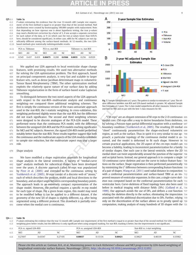
Fig. 7. Sample Size Estimates at 2 years. The pattern is similar to estimates at 1 year. The rel-ative difference between stat-ROI and LDA-based methods is greater. NC-adjusted SampleSize Estimates at 2 years. The 2-class model outperforms all other measures. Volume is sec-ond best for MCI and on par with the best 1-class measures for AD.



UNCO

RRECTED P

RO

OF722 continuous medial axis achievable in little timewithout using large com-

723 puting clusters.

724 Machine learning in shape analysis and Alzheimer's disease

725 PCA-type approaches have been used in prior shape analyses. A726 regularized components analysis approach called LoCA (Alcantara et727 al., 2009) is similar to sparse PCA (Zou et al., 2006). The idea, similar728 to PCA, is to generate an orthogonal basis for shape space, while729 adding a penalty term. However, instead of penalizing the number730 of non-zero weights in each basis vector, as is done in sparse PCA,731 LoCA instead forces all the non-zero components to be spatially clus-732 tered on a surface, which gives each component a clearer anatomical733 meaning. However, both of these methods come at a much higher734 computational cost than ordinary PCA: they are iterative, while PCA735 only relies on eigen-decomposition, making it feasible for much larg-736 er feature sets. LoCA has been applied to shape analysis in AD, includ-737 ing ADNI hippocampal data (Carmichael et al., 2012), finding specific738 component associations with AD and other biomarkers. Here, the739 measure used was very similar to ours, the radial distance. Only base-740 line data were used in assessing morphometric differences, while our741 current study is longitudinal.742 Sparse basis decomposition has also been used as a preprocessing743 step for training an AD classifier, for example by applying Independent744 Component Analysis (ICA) to gray matter density maps before using745 machine learning methods, such as Support Vector Machines (SVM),746 for classification (Yang et al., 2010).Manymachine learning approaches747 have been applied to image-based diagnosis or classification of AD and748 MCI. Davatzikos and colleagues applied SVM to RAVENS maps (Fan et749 al., 2008), an approach similar to modified VBM (Good et al., 2002)750 which assigns relative tissue composition to every voxel after a751 high-dimensional warp. A similar approach was used by Vemuri et al.

752(2008), using tissue probability maps (TPMs)—essentially the same753VBM measures that are constructed using the SPM package. Kloppel et754al. (2008) further showed that such a model can be stable across differ-755ent datasets. In general, classification algorithms can achieve AD-NC756cross-validation accuracy in the mid-nineties (~95%) within the same757dataset, although performance inevitably degrades when applied to758new datasets, especially if the cohort demographics or scanning proto-759cols are different.760Cuingnet et al. (2010) developed a Laplacian-regularized SVM ap-761proach for classifying AD and NC subjects, which is very similar in762spirit to our Tikhonov-regularized LDA. They show that using the763Laplacian regularizer improves classification rates for AD vs. NC sub-764jects. SVM has also been used, in our prior work, to separate AD and765NC subjects based on hippocampal shape invariants and spherical766harmonics (Gutman et al., 2009). Another recent surface-based classi-767fication effort by Cho et al. (2012) uses an approach very similar to768our PCA method, where surface atlas-registered cortical thickness769data is smoothed with a low-pass filter of the Laplace-Beltrami oper-770ator, computed on the atlas shape. Following this procedure, PCA is771performed on the smoothed surface thickness data and LDA is772performed on a subset of the PCA coefficients to train a linear classifi-773er. The resulting classification accuracy is very competitive. Another774surface-based classifier (Gerardin et al., 2009) uses the SPHARM-775PDM approach to classify AD and NC subjects based on hippocampal776shape. SPHARM-PDM (Styner et al., 2005) computes a small number777of spherical harmonic coefficients based on an area-preserving sur-778face map, and normalizes the spherical correspondence by aligning779the first-order ellipsoid with the poles. The result is a rudimentary780surface registration and a spectral decomposition of the shape.781Gerardin et al. reported competitive classification rates compared to782whole-brain approaches. Shen et al. (2010) recently used a Bayesian783feature selection approach and classification on cortical thickness

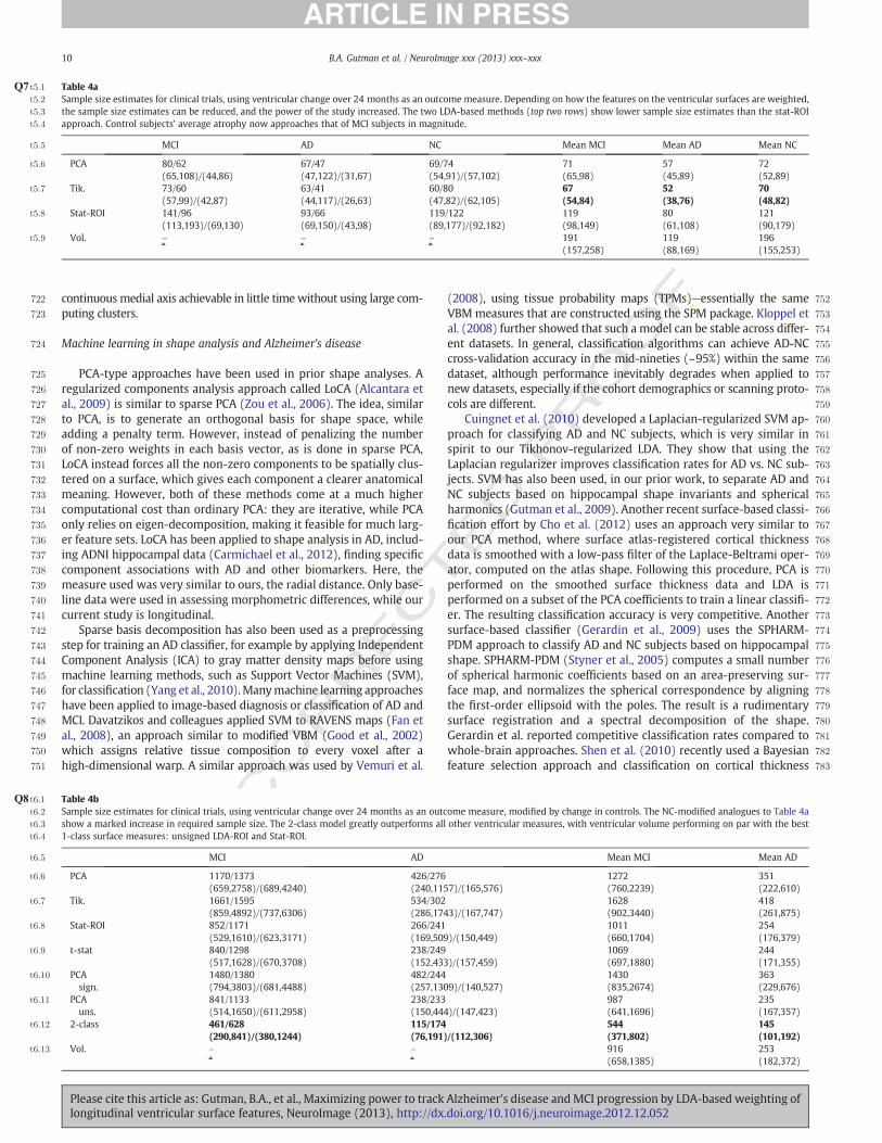
Q7 Table 4at5:1

t5:2 Sample size estimates for clinical trials, using ventricular change over 24 months as an outcome measure. Depending on how the features on the ventricular surfaces are weighted,t5:3 the sample size estimates can be reduced, and the power of the study increased. The two LDA-based methods (top two rows) show lower sample size estimates than the stat-ROIt5:4 approach. Control subjects' average atrophy now approaches that of MCI subjects in magnitude.

t5:5 MCI AD NC Mean MCI Mean AD Mean NC

t5:6 PCA 80/62(65,108)/(44,86)

67/47(47,122)/(31,67)

69/74(54,91)/(57,102)

71(65,98)

57(45,89)

72(52,89)

t5:7 Tik. 73/60(57,99)/(42,87)

63/41(44,117)/(26,63)

60/80(47,82)/(62,105)

67(54,84)

52(38,76)

70(48,82)

t5:8 Stat-ROI 141/96(113,193)/(69,130)

93/66(69,150)/(43,98)

119/122(89,177)/(92,182)

119(98,149)

80(61,108)

121(90,179)

t5:9 Vol. – – – 191(157,258)

119(88,169)

196(155,253)

Q8 Table 4bt6:1

t6:2 Sample size estimates for clinical trials, using ventricular change over 24 months as an outcome measure, modified by change in controls. The NC-modified analogues to Table 4at6:3 show a marked increase in required sample size. The 2-class model greatly outperforms all other ventricular measures, with ventricular volume performing on par with the bestt6:4 1-class surface measures: unsigned LDA-ROI and Stat-ROI.

t6:5 MCI AD Mean MCI Mean AD

t6:6 PCA 1170/1373(659,2758)/(689,4240)

426/276(240,1157)/(165,576)

1272(760,2239)

351(222,610)

t6:7 Tik. 1661/1595(859,4892)/(737,6306)

534/302(286,1743)/(167,747)

1628(902,3440)

418(261,875)

t6:8 Stat-ROI 852/1171(529,1610)/(623,3171)

266/241(169,509)/(150,449)

1011(660,1704)

254(176,379)

t6:9 t-stat 840/1298(517,1628)/(670,3708)

238/249(152,433)/(157,459)

1069(697,1880)

244(171,355)

t6:10 PCAsign.

1480/1380(794,3803)/(681,4488)

482/244(257,1309)/(140,527)

1430(835,2674)

363(229,676)

t6:11 PCAuns.

841/1133(514,1650)/(611,2958)

238/233(150,444)/(147,423)

987(641,1696)

235(167,357)

t6:12 2-class 461/628(290,841)/(380,1244)

115/174(76,191)/(112,306)

544(371,802)

145(101,192)

t6:13 Vol. – – 916(658,1385)

253(182,372)



UNCO

RRECTED P

RO

OF784 data and showed that AD-NC and MCI-NC classification accuracy re-

785 mains competitive with SVM. Finally, to combine multiple modalities786 for classification, Zhang et al. (2011) developed a multiple kernel SVM787 classifier to further improve diagnostic AD and MCI classification.788 It is important to stress that while many studies have used machine789 learning to derive a single measure of “AD-like” morphometry for790 discriminating AD and MCI subjects from the healthy group, no study791 we are aware of has used machine learning to maximize the power of792 absolute atrophy rates in AD. We have attempted this by using a straight-793 forward application of LDA, using either PCA or Tikhonov regularization.794 The Tikhonov approach was intended to improve generalization relative795 to PCA, but surprisingly, there were essentially no major differences in

796test sample size estimates for AD and MCI subjects between the two797methods. Only one subgroup at 24 months approached a trend level for798a difference in efficiency (sample size difference) between the Tikhonov799and PCA model. The Tikhonov method was slightly better for reducing800sample size estimates in MCI, generalizing better - as expected. A poten-801tial cause of this may be an insufficiently thorough optimal parameter802search for the Tikhonov approach, as the searchmust remain fairly coarse803due to computational constraints. On theother hand, it is possible that the804covariance structure of the training samples captures the spatial priors805sufficiently well, and an explicit prior does not significantly improve806generalizability.807Outside of Alzheimer's literature we found one approach for ex-808plicitly minimizing sample size estimates (Qazi et al., 2010), and809another that uses SVM for classification of Huntington's disease pa-810tients versus controls, with reduced sample sizes as a by-product811(Hobbs et al., 2010). The first paper is methodologically closest in812spirit to this work: a fidelity term is explicitly defined to be the813control-adjusted sample size estimate. A number of non-linear814constraints are then added: the total variation norm (TV1-norm),815sparsity and non-negativity. While the first two have analogues816that can be linearly optimized as we do here (TV2 and L2 norm),817the third constraint forces the authors to use non-linear conjugate818gradient (CG), which leads to far slower convergence than the lin-819ear CG we use. More importantly, due to the differences in the na-820ture of their data—knee cartilage CT images—and ours, the sparsity821and non-negativity constraints are perhaps not appropriate for

Fig. 8. Regression plots for surface-based ventricular expansion measures in controls. 95% confidence belts for the regression models are shown with dotted green lines. All surfacemodels are longitudinally unbiased, since the zero intercept is contained in the 95% confidence interval on the intercept, for each of the methods. The 2-class model is trending onadditive bias; however, in this model the mean of controls is subtracted for power estimates.

Q9 Table 5t7:1

t7:2 P-values estimating the chance that the true 24 month n80 of the first method is equalt7:3 to or greater than that of the second method. Null distributions were created byt7:4 bootstrapping 100,000 samples with replacement. Note that depending on how rigor-t7:5 ous one is about hypothesis testing, the true p-values may need a Bonferroni correctiont7:6 by a factor of 3, if one accepts a separate correction for each subset of the data, or 9. Thet7:7 improvement of the Tikhonov-LDA method over the stat-ROI approach reaches signif-t7:8 icance, when uncorrected, for AD subjects. At 24 months, the improvement in powert7:9 when using Tikhonov-regularized LDA model over the PCA model approaches trendt7:10 levels for MCI subjects.

t7:11 Tikhonov vs. PCA PCA vs. stat-ROI Tikhonov vs. stat-ROI


t7:13 0.129 0.257 0.334 0.00249 0.11 0.00278 0.0001 0.0276 0.00076



P

UNCO

RRECTED P

RO

OF

822 brain imaging. We expect the effect over soft tissue to be diffuse823 without many discontinuities, and non-negativity is generally not824 appropriate in brain MR either. Admittedly, though, as we have825 focused only on the ventricles, non-negativity would probably be826 appropriate here, though it would lead to slower convergence.827 The second paper (Hobbs et al., 2010), which we mention in the in-828 troduction, simply uses leave-one-out linear SVM weighting of829 fluid registration-based TBM maps to derive an atrophy measure.830 No spatial regularization, or sample size-specific modification to831 the learning approach is used. In both of these cases the measure832 used is based on the difference between the mean of controls and833 the diseased group, which is not the main goal of the present834 work. Though we have used the NC-adjusted measure here as835 well to show the potential to reveal AD-specific ventricular change836 patterns, the main goal was to optimize detection of absolute837 change.

838 Other ventricular measures

839 Several studies have used a ventricularmeasure alone, as a predictor840 of cognitive decline. Ott et al. (2010) showed that ventricular volume is841 associated with CSF Aβ. Carmichael et al. (2007) compared ventricular842 volume and ventricle–brain ratio (VBR) across MCI converters and843 non-converters with significantly increased volume, and VBR at base-844 line among converters. Nestor et al. (2008) used a semi-automated845 highly precise ventricular segmentation to estimate differences in846 rates of volumetric change. Rates of volumetric increase in the ventri-847 cles were significantly greater in MCI and AD subjects compared to848 NC, which is in line with expectations about the rates of atrophy in849 each group. Chou et al. (2009) performed a cross-sectional ventricular850 study on the baseline ADNI dataset, using a surface-based model. Sur-851 faces were registered—in a similar way to Thompson et al. (2004)—by852 separating each horn and computing three separate medial axes. The853 radial distance measure was shown to be significantly different be-854 tween NC and AD, and NC and MCI subjects. Several other cognitive855 measures and CSF biomarkers were shown to correlate significantly856 with the local ventricular surface expansion, in a direction expected857 from the advancing pathology and the intensification of the disease.858 Ferrarini et al. (2006) showed differences in local ventricular surface859 morphometry between AD and NC subjects using permutations testing860 and a novel algorithm—known as “GAMEs”—for surface meshing and861 matching.

862 Power estimates of other measures in AD

863 Our ventricular change measures outperformed other common ven-864 tricularmeasures as an AD biomarker with respect to the sample size re-865 quirements, assuming of course that the reference data are comparable.866 Schott et al. (2010) reported 1-year n80s for the “Ventricular Boundary867 Shift Integral” (VBSI) of 118 (92, 157) for AD and 234 (191,295) for868 MCI at 1 year. Holland et al. (2011) reported a Quarc ventricle measure869 of 92 (69, 135) for AD and 183 (146, 241) for MCI for a 2-year trial.870 FreeSurfer ventricular measures give similar 2-year estimates of 90871 (68,128) for AD and 164 (133, 211) for MCI. Our approach performs872 comparably well or better thanmany other imagingmeasures, in partic-873 ular those using the entire cortex. An FSL tool, known as SIENA (Smith et874 al., 2002; Cover et al., 2011), achieved a 1-year point estimate for sample

875size of 132 for AD and 278 for MCI. Quarc achieved 2-year whole brain876estimates of 84 (63, 123) for AD and 149 (121, 193) for MCI. FreeSurfer877is reported (Holland et al., 2011) to achieve 2-yearwhole brain estimates878of 252 (175, 408) for AD and 384 (294, 531) forMCI. Schott reported that879BBSI, awhole brain graymatter atrophymeasure (Schott et al., 2010), re-880quired 1-year samples of 81 (64, 109) for AD and 149 (122, 188) forMCI.881Huaet al. (2012) used improved Tensor BasedMorphometry (TBM)with882the stat-ROI voxelweighting to achieve 1-year sample sizes of 58 (45,81)883for AD and 124 (98,160) for MCI. These comparisons are summarized in884Figs. 9 and 10. Though all sample size estimates mentioned here are885based on the same ADNI-1 dataset, different studies were done on886ADNI subsamples of different size. To shed some light on this, we give887the number of subjects used for each study in Table 8. Comparison888between our study and others is more meaningful where there are889fewer exclusions. We note that while the Quarc and Freesurfer results890fromHolland et al. (2011) are for a 2-year study, and using a slightly dif-891ferent power calculation, in fact even subjects who only had scans up to8921 year were considered. The variance and disease effect in these calcula-893tions were based on a mixed effect model using all available time points894for each subject. However, there are still roughly 10% fewer subjects used895for Quarc and 7% fewer for Freesurfer compared to the full ADNI dataset.

896Algorithmic bias

897Importantly, we showed that our surface-based measures are lon-898gitudinally unbiased according to the intercept CI test (Yushkevich et899al., 2010), alleviating common concerns about overly optimistic sam-900ple size estimates due to, for example, additive algorithmic bias. The901fact that the baseline and follow-up scans were processed identically,902and independently, avoids several sources of subtle bias in longitudi-903nal image processing that can arise from not handling the images in a904uniform way (Thompson and Holland, 2011). Some issues have been905raised regarding the validity of the intercept CI test as a test for bias in906estimating rates of change. The CI test assumes that the true morpho-907metric change from baseline increases in magnitude linearly over908time in healthy controls. Relying on this assumption, the test exam-909ines whether the intercept of the linear model, fitted through mea-910sures of change at successive time intervals in controls, is zero. If911this is not the case, the measure of change is said to have additive912bias. There are two common criticisms of this test. First, the linearity913assumption may not always be valid, i.e., true biological changes may914be nonlinear. In this case, a truly unbiased algorithm could fail the915test, while giving accurate results. For example, the loss of tissue916may be proportional to the amount of tissue left, so the change in917volume as measured by TBM, or medial distance to a ventricular918boundary relative to baseline might decay or expand exponentially.919Alternatively, if loss of tissue volume is linear in time, radial distance920measures might be expected to change in proportion to the cube-root921of time, or to vary according to some empirical power law relating the922distance to volumetric measures, depending on which directional923changes contribute most to the overall change (Zhang and Sejnowski,9242000; Brun et al., 2009). This may partially explain the slight additive925“bias” that is detectable in AD andMCI subjects (though not in controls).926In disease, the power law describing changes as a function of time may927be different compared to controls due to disease effects. As a result, only928control subjects should be used when using the linear fit CI test, but

Table 6t8:1

t8:2 Longitudinal bias analysis of ventricular surface-based measures. Change in healthy controls is linearly regressed over two time points. The intercept is very close to zero, with thet8:3 confidence interval clearly containing zero for each method. The surface-based measures do not show any algorithmic bias according to the CI test.

t8:4 PCA Tikhonov T-stat 2-classLDA

Signed LDA-ROI Unsigned LDA-ROI Stat-ROI

t8:5 0.0064(−0.0218, 0.06)

0.0048(−0.0126, 0.0242)

−0.0102(−0.0617, 0.0416)

0.0172(−0.0031, 0.036)

−0.0031(−0.0208, 0.0143)

−0.0189(−0.0665, 0.0304)

0.0115(−0.0411, 0.0645)



UNCO

RRECTED P

RO

OF

929even in that case, it is not a perfect test, in that an accurate algorithm930could fail the test.931The second common criticism of the CI bias test is that non-932additive, atrophy-dependent type of bias may not be detected with933the test. In other words, if there exists a complex transfer function be-934tween the true change and measured change, a simple linear regres-935sion through several time points may not reveal this as a non-zero936y-intercept. However, care must be taken when such a transfer func-937tion is discovered in an algorithm. It is not simply enough to show the938existence of such a function to call an algorithm “biased”; one must939also show that the function systematically scales the square of the940mean and the variance of the whole sample differently over any num-941ber of time points. To address this, we will break the possible transfer942functions into four somewhat-overlapping categories, ordered by943plausibility, and discuss each. We assume that in all cases an observed944transfer function for the mean change is similar in form to the true945transfer function for individual subjects.

9461. No additive bias and a transfer function whose second derivative has the947same sign everywhere. This is perhaps the most likely scenario. For948example, measures derived from non-linear deformation fields949such as TBM are known to undergo this kind of bias when950inverse-consistency is not enforced; page 5 of Tagare et al. (2009)951gives a clear explanation for this. In this case, assuming a linear952true change, the measured change will follow a non-decreasing (or953non-increasing) curve with the same convexity everywhere. Since954we assume a zero y-intercept for the curve, a linear fit through two955or more time points will inevitably show a non-zero intercept,956given enough true change. Thus, the CI intercept test can detect957this kind of bias even with just two time points in addition to base-958line. Most “known” cases of algorithmic bias that the CI test has so959far revealed in literature (Yushkevich et al., 2010; Holland et al.,9602011) may well fall in this category.9612. An additive bias and a transfer function whose second derivative has962the same sign everywhere. In this case, the additive bias may indeed963cancel out the effect of the atrophy-dependent bias, if the second964derivative and the additive bias have the same sign. However,965this would require quite a special set of circumstances: the sam-966pled time-points and the additive portion of the bias would have967to be just right for the linear fit to have a zero y-intercept. With968sufficiently many time points, this situation becomes virtually im-969possible. However, as we have only used three time points, we970must admit that this is a possibility, however unlikely, in our study.9713. A strictly linear transfer function with or without additive bias. This972scenario is the clearest example of when the CI test would fail. In973this case, the measured mean change would be a constant multiple974of true mean change. However, it is unclear whether this kind of975transfer function can be properly called a “bias.” If such a transfer976function had similar form for individual subjects as their sample977mean, the sample size estimates would remain unchanged, as the978variance would scale in the same way as the square of the mean.979On the other hand, it is somewhat difficult to imagine a linear980bias that scales the variance and the square of the mean differently981for many time points. This would violate our assumption.9824. “Other:” A transfer function with one or more inflection points, with983or without additive bias. Though experience with image processing984algorithms shows that this scenario is highly improbable, in the985interest of completeness we note that this kind of bias can indeed986be missed by the CI test, while unfairly inflating power estimates.987This is also the only scenario in which our assumption regarding988individual bias and bias of the mean will be invalid.

989Having gone through this exercise, we hope to have shown that990while certain kinds of non-additive bias can potentially be left991undetected by the intercept CI test, such a bias is either improbable992or does not lead to unfair sample size estimation. Far more likely is993the breakdown in the linearity assumption of the CI test, which

Q10

Table7a

t9:1

t9:2

Ven

tricular

surfacesu

mmaryatroph

ymea

suresforco

ntinuo

usweigh

ting

s.Ave

rage

san

dstan

dard

deviations

foratroph

yratesarein

millim

etersof

radial

expa

nsion.

Theve

rtex

weigh

tsareno

rmalized

bytheir1-no

rm,w

hich

correspo

ndsto

t9:3

averag

ingov

ertheRO

Ifor

thestat-R

OIm

etho

d,assu

mingeq

uala

reaelem

ents

forallv

ertices.

t9:4

Tikh

onov

PCA

t-stat

2-classLD

A

t9:5

MCI

AD

NC

MCI

AD

NC

MCI

AD

NC

MCI

AD

NC

t9:6

12mo

0.08

72±

0.06

00.10

5±

0.06

20.07

04±

0.05

40.15

1±

0.10

0.19

1±

0.11

0.11

1±

0.08

40.24

7±

0.21

0.34

9±

0.21

0.14

6±

0.14

0.05

8±

0.06

0.08

35±

0.07

30.02

99±

0.05

t9:7

24mo

0.14

6±

0.07

90.18

1±

0.08

60.13

5±

0.06

70.25

7±

0.14

0.33

±0.17

0.21

4±

0.11

0.46

±0.32

0.68

±0.37

0.30

4±

0.21

0.10

1±

0.1

0.17

5±

0.13

0.04

12±

0.08



UNCO

RRECTED P

RO

OF

994 renders the test inappropriate. Using a subset of the data in which the995 change is small enough to be at least approximately linear in time, i.e.996 the control subjects, alleviates the latter issue.997 We deliberately chose to use only 12-month data in training our998 optimized atrophy models. This choice was motivated by practical999 concerns: we wanted to show that using LDA for optimizing power1000 generalizes sufficiently well to later time points without requiring1001 real drug trials to recompute the atrophy measure for all scans with1002 each new batch of data. This latter situation could be considered a1003 “moving target.”While it may be argued that a better, more parsimoni-1004 ous model could be trained on a sample that includes all available time1005 points, perhaps even incorporating the time variable explicitly, such an1006 approach potentially hides anymethodological bias that is inherent in a1007 particular algorithm. Further, a real clinical trial would likely require an1008 ability to apply the same measure to new follow-up scans without1009 requiring one to recompute the measure for all time points every time1010 a new batch of follow-up scans becomes available. In this way, we1011 avoid the moving target problem that bedevils methods requiring1012 scans from all time points. Further, because such methods rely on1013 data-driven techniques to reduce longitudinal bias, for example by1014 computing a per-subject brain atlas based on all available time points,1015 the perceived absence of bias does not indicate that the imaging algo-1016 rithms themselves are unbiased. This may be called a kind of “peaking”

1017or circularity, as the data used to assess the bias is also used to compute1018the atrophymeasure. However, we do not rely on any data-driven tech-1019niqueswhich explicitly force the results to be transitive over time for all1020available scans. In this sense, the absence of bias in our measures is1021more indicative of algorithmic objectivity with respect to the amount1022and direction of morphometric change.

1023Total and relative atrophy

1024There has been some recent debate regarding the need to subtract1025the mean of the healthy controls when estimating sample sizes for a1026drug trial. Some ADNI collaborators seem to have rejected this idea1027(Hua et al., 2012; Wyman et al., accepted for publication), in part be-1028cause real drug trials do not tend to enroll controls, and even if they1029did, many controls already harbor incipient Alzheimer pathology or1030some degree of vascular pathology that may also be resisted by treat-1031ment. However, the idea is not completely without merit, since all1032meaningful trials must compare a treatment against another (placebo1033or established) treatment group. Further, any additive algorithmic1034bias could be excluded by subtracting the mean rate of controls. In1035this paper, we addressed this issue by computing an additional linear1036ventricular expansion model, specific to AD and MCI progression. We1037did this by directly applying a 2-class, as opposed to 1-class, LDA with1038the covariance defined strictly by the diseased group, as required by1039the current practice of NC-adjusted sample size estimates. The1040resulting power estimates for NC-adjusted atrophy outperform all1041previous ventricular measures.

1042Future work

1043Future work will include combination of multiple biomarkers, in-1044cluding other imaging biomarkers, such as TBM or even non-imaging1045biomarkers (such as CSF or proteomic measures), into the framework.1046For example, there is no mathematical reason why only the ventricular1047measures should be included, as any pertinent structural or functional1048measure could be incorporated. In the former case, only the PCA-1049based approach would be feasible due to the high computational cost.1050It is also important to validate the LDA-weighted measures as well as

Q2 Table 7bt10:1

t10:2 Ventricular surface summary atrophy measures for discrete weightings. Discrete analogues of results in Table 7a, because negative weights are allowed in signed LDA-ROI, the nor-t10:3 malized average expansion is closer to the 2-class LDA result, while the unsigned version is closer to stat-ROI and t-statistic weighting.

t10:4 stat-ROI Signed LDA-ROI Unsigned LDA-ROI


t10:6 12 months 0.262±0.21 0.367±0.22 0.158±0.14 0.0602±0.042 0.0796±0.046 0.0411±0.035 0.226±0.2 0.328±0.2 0.132±0.13t10:7 24 months 0.468±0.32 0.690±0.39 0.306±0.21 0.108±0.06 0.14±0.068 0.083±0.046 0.438±0.3 0.652±0.36 0.284±0.19

Fig. 9. A. Sample size estimates for different ventricular biomarkers. The PCAmethod is des-ignated here as “Medial Vent-LDA.” The Quarc and Freesurfer measures are for a two-yeartrial. B. NC-adjusted Sample size estimates for different ventricular biomarkers. The 2-classPCA method is designated here as “Medial Vent-LDA.” All other results are taken fromHolland et al. (2011).

Fig. 10. Sample size estimates for differentwhole biomarkers compared to our ventricularmeasure. The PCA method applied to ventricular surfaces is designated here as “MedialVent-LDA.” The Quarc and Freesurfer measures are for a 2-year trial. SIENA estimatesare computed from the means and variances reported in Cover et al. (2011).



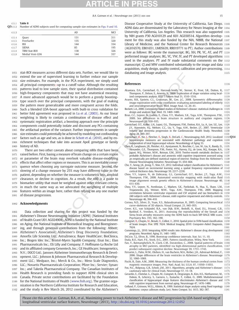
UNCO

RRECTED P

RO

OF

1051 stat-ROI measures across different data sets. Further, we would like to1052 extend the use of supervised learning to further reduce our sample1053 size estimates. For example, in the PCA experiment, we simply used1054 all principal components—up to a cutoff value. Although the resulting1055 patterns lead to low sample sizes, their spatial distribution contained1056 high-frequency components that may not have anatomical meaning.1057 A more advanced approach would be to perform a greedy boosting-1058 type search over the principal components, with the goal of making1059 the pattern more generalizable and more congruent across the folds.1060 Such a blended LDA-boost approach with built-in cross validation for1061 better fold agreement was proposed in Lu et al. (2003). As our linear1062 weighting is likely to contain a combination of disease effect and1063 systematic registration artifact, a boosting approach over the principle1064 components could potentially isolate and discount any PCs containing1065 the artifactual portion of the variance. Further improvements in sample1066 size estimates could potentially be achievedbymodeling out confounding1067 factors such as age and sex, as is done in Schott et al. (2010), and by en-1068 richment techniques that take into account ApoE genotype or family1069 history of AD.1070 There are two other caveats about comparing n80s that have been1071 raised before. First, basing ameasure of brain change on a certain region1072 or parameter of the brain may overlook valuable disease-modifying1073 effects that affect other regions ormeasures. This is an inevitable conse-1074 quence when choosing any surrogate outcome measure. Second, the1075 slowing of a change measure by 25% may have different value to the1076 patient, depending on whether the measure is volumetric loss, amyloid1077 clearance, or decline in cognition. As a result, the n80 is a guide to1078 biomarker utility that must be weighed against other relevant criteria,1079 in much the same way as we advocated the weighting of multiple1080 features within an image here, rather than relying on any one marker1081 of disease progression.

1082 Acknowledgments

1083 Data collection and sharing for this project was funded by the1084 Alzheimer's Disease Neuroimaging Initiative (ADNI) (National Institutes1085 of Health Grant U01 AG024904). ADNI is funded by the National Institute1086 on Aging, the National Institute of Biomedical Imaging and Bioengineer-1087 ing, and through generous contributions from the following: Abbott;1088 Alzheimer's Association; Alzheimer's Drug Discovery Foundation;1089 Amorfix Life Sciences Ltd.; AstraZeneca; Bayer HealthCare; BioClinica,1090 Inc.; Biogen Idec Inc.; Bristol-Myers Squibb Company; Eisai Inc.; Elan1091 Pharmaceuticals Inc.; Eli Lilly and Company; F. Hoffmann-La Roche Ltd1092 and its affiliated company Genentech, Inc.; GEHealthcare; Innogenetics,1093 N.V.; IXICO Ltd.; Janssen Alzheimer Immunotherapy Research & Devel-1094 opment, LLC.; Johnson & Johnson Pharmaceutical Research & Develop-1095 ment LLC.; Medpace, Inc.; Merck & Co., Inc.; Meso Scale Diagnostics,1096 LLC.; Novartis Pharmaceuticals Corporation; Pfizer Inc.; Servier; Synarc1097 Inc.; and Takeda Pharmaceutical Company. The Canadian Institutes of1098 Health Research is providing funds to support ADNI clinical sites in1099 Canada. Private sector contributions are facilitated by the Foundation1100 for the National Institutes of Health (www.fnih.org). The grantee orga-1101 nization is the Northern California Institute for Research and Education,1102 and the study is Rev March 26, 2012 coordinated by the Alzheimer's

1103Disease Cooperative Study at the University of California, San Diego.1104ADNI data are disseminated by the Laboratory for Neuro Imaging at the1105University of California, Los Angeles. This research was also supported1106by NIH grants P30 AG010129 and K01 AG030514. Algorithm develop-1107ment for this study was also funded by the NIA, NIBIB, the National1108Library of Medicine, and the National Center for Research Resources1109(AG016570, EB01651, LM05639, RR019771 to PT). Author contributions1110were as follows: BG wrote the manuscript; BG, XH, PR, YC, AT, and PT1111performed image analyses; BG, YC, YW, IY, and PT developed algorithms1112used in the analyses. PT and IY made substantial comments on the1113manuscript; CJ and MW contributed substantially to the image and data1114acquisition, study design, quality control, calibration and pre-processing,1115databasing and image analysis.

1116References

1117Alcantara, D.A., Carmichael, O., Harcourt-Smith, W., Sterner, K., Frost, S.R., Dutton, R.,1118Thompson, P., Delson, E., Amenta, N., 2009. Exploration of shape variation using local-1119ized components analysis. IEEE T Pattern Anal 31, 1510–1516.1120Avants, B.B., Epstein, C.L., Grossman, M., Gee, J.C., 2008. Symmetric diffeomorphic1121image registration with cross-correlation: evaluating automated labeling of elderly1122and neurodegenerative brain. Med. Image Anal. 12, 26–41.1123Beckett, L.A., 2000. Community-based studies of Alzheimer's disease: statistical challenges in1124design and analysis. Stat. Med. 19, 1469–1480.1125Brun, C.C., Lepore, N., Luders, E., Chou, Y.Y., Madsen, S.K., Toga, A.W., Thompson, P.M.,11262009. Sex differences in brain structure in auditory and cingulate regions.1127Neuroreport 20, 930–935.1128Carmichael, O.T., Kuller, L.H., Lopez, O.L., Thompson, P.M., Dutton, R.A., Lu, A., Lee, S.E., Lee,1129J.Y., Aizenstein, H.J., Meltzer, C.C., Liu, Y., Toga, A.W., Becker, J.T., 2007. Ventricular1130volume and dementia progression in the Cardiovascular Health Study. Neurobiol.1131Aging 28, 389–397.1132Q14Carmichael, O., Xie, J., Fletcher, E., Singh, B., DeCarli, C., Neuroimaging AsD, 2012. Localized1133hippocampus measures are associated with Alzheimer pathology and cognition1134independent of total hippocampal volume. Neurobiology of Aging 33.1135Chen, K., Langbaum, J.B., Fleisher, A.S., Ayutyanont, N., Reschke, C., Lee, W., Liu, X., Bandy, D.,1136Alexander, G.E., Thompson, P.M., Foster, N.L., Harvey, D.J., de Leon, M.J., Koeppe, R.A.,1137Jagust, W.J., Weiner, M.W., Reiman, E.M., 2010. Twelve-month metabolic declines in1138probable Alzheimer's disease and amnestic mild cognitive impairment assessed using1139an empirically pre-defined statistical region-of-interest: findings from the Alzheimer's1140Disease Neuroimaging Initiative. Neuroimage 51, 654–664.1141Cho, Y., Seong, J.K., Jeong, Y., Shin, S.Y., 2012. Individual subject classification for Alzheimer's1142disease based on incremental learning using a spatial frequency representation of1143cortical thickness data. Neuroimage 59, 2217–2230.1144Chou, Y.Y., Lepore, N., de Zubicaray, G.I., Carmichael, O.T., Becker, J.T., Toga, A.W.,1145Thompson, P.M., 2008. Automated ventricular mapping with multi-atlas fluid1146image alignment reveals genetic effects in Alzheimer's disease. Neuroimage 40,1147615–630.1148Chou, Y.Y., Lepore, N., Avedissian, C., Madsen, S.K., Parikshak, N., Hua, X., Shaw, L.M.,1149Trojanowski, J.Q., Weiner, M.W., Toga, A.W., Thompson, P.M., 2009. Mapping1150correlations between ventricular expansion and CSF amyloid and tau biomarkers in1151240 subjects with Alzheimer's disease, mild cognitive impairment and elderly controls.1152Neuroimage 46, 394–410.1153Cornea, N.D., Silver, D., Yuan, X.S., Balasubramanian, R., 2005. Computing hierarchical1154curve-skeletons of 3D objects. Visual Comput. 21, 945–955.1155Cover, K.S., van Schijndel, R.A., van Dijk, B.W., Redolfi, A., Knol, D.L., Frisoni, G.B.,1156Barkhof, F., Vrenken, H., 2011. Assessing the reproducibility of the SienaX and1157Siena brain atrophy measures using the ADNI back-to-back MP-RAGE MRI scans.1158Psychiatry Res. 193, 182–190.1159Cuingnet, R., Chupin, M., Benali, H., Colliot, O., 2010. Spatial prior in SVM-based classification1160of brain images. Proc SPIE 7624: Medical Imaging 2010: Computer-Aided Diagnosis,11617624.1162Cummings, J.L., 2010. Integrating ADNI results into Alzheimer's disease drug development1163programs. Neurobiol. Aging 31, 1481–1492.1164DiCicio, T.J., Efron, B., 1996. Bootstrap confidence intervals. Stat. Sci. 11, 10.1165Duda, R.O., Hart, P.E., Stork, D.G., 2001. Pattern classification. Wiley, New York.1166Fan, Y., Batmanghelich, N., Clark, C.M., Davatzikos, C., 2008. Spatial patterns of brain1167atrophy in MCI patients, identified via high-dimensional pattern classification,1168predict subsequent cognitive decline. Neuroimage 39, 1731–1743.1169Ferrarini, L., Palm, W.M., Olofsen, H., van Buchem, M.A., Reiber, J.H., Admiraal-Behloul, F.,11702006. Shape differences of the brain ventricles in Alzheimer's disease. Neuroimage117132, 1060–1069.1172Fischl, B., Dale, A.M., 2000. Measuring the thickness of the human cerebral cortex from1173magnetic resonance images. Proc. Natl. Acad. Sci. U.S.A. 97, 11050–11055.1174Fox, N.C., Ridgway, G.R., Schott, J.M., 2011. Algorithms, atrophy and Alzheimer's disease:1175cautionary tales for clinical trials. Neuroimage 57, 15–18.1176Gerardin, E., Chetelat, G., Chupin, M., Cuingnet, R., Desgranges, B., Kim, H.S., Niethammer, M.,1177Dubois, B., Lehericy, S., Garnero, L., Eustache, F., Colliot, O., 2009. Multidimensional1178classification of hippocampal shape features discriminates Alzheimer's disease and1179mild cognitive impairment from normal aging. Neuroimage 47, 1476–1486.1180Golland, P., Grimson, W.E.L., Kikinis, R., 1999. Statistical shape analysis using fixed topology1181skeletons: corpus callosum study. Lect. Notes Comput. Sci. 1613, 382–387.

Table 8t11:1

t11:2 Number of ADNI subjects used for computing sample size estimates in Figs. 9 and 10.Q3

t11:3 AD MCI

t11:4 Quarc 131 311t11:5 FreeSurfer 135 320t11:6 BSI 144 334t11:7 SIENA 85 195t11:8 TBM Stat-ROI 138 326t11:9 Medial Vent-LDA 144 337



troopo

Ed

i 624

UNCO

RRECTED P

RO

OF

1182 Good, C.D., Scahill, R.I., Fox, N.C., Ashburner, J., Friston, K.J., Chan, D., Crum, W.R., Rossor,1183 M.N., Frackowiak, R.S., 2002. Automatic differentiation of anatomical patterns in1184 the human brain: validation with studies of degenerative dementias. Neuroimage1185 17, 29–46.1186 Gunter, J., Bernstein, M., Borowski, B., Felmlee, J., Blezek, D., Mallozzi, R., Levy, J., Schuff,1187 N., Jack Jr., C.R., 2006. Validation testing of the MRI calibration phantom for the1188 Alzheimer's Disease Neuroimaging Initiative Study. ISMRM 14th Scientific Meeting1189 and Exhibition.1190 Gutman, B., Wang, Y., Morra, J., Toga, A.W., Thompson, P.M., 2009. Disease classification1191 with hippocampal shape invariants. Hippocampus 19, 572–578.1192 Gutman, B.A., Yalin, W., Rajagopalan, P., Toga, A.W., Thompson, P.M., 2012. Shape1193 matching with medial curves and 1-D group-wise registration. Biomedical Imaging1194 (ISBI), 2012 9th IEEE International Symposium on, pp. 716–719.1195 Hobbs, N.Z., Henley, S.M.D., Ridgway, G.R., Wild, E.J., Barker, R.A., Scahill, R.I., Barnes, J., Fox,1196 N.C., Tabrizi, S.J., 2010. The progression of regional atrophy in premanifest and early1197 Huntington's disease: a longitudinal voxel-based morphometry study. J. Neurol.1198 Neurosurg. Psychiatry 81, 756–763.1199 Holland, D., Dale, A.M., 2011. Nonlinear registration of longitudinal images and measure-1200 ment of change in regions of interest. Med. Image Anal. 15, 489–497.1201Q15 Holland, D., McEvoy, L.K., Dale, A.M., 2011. Unbiased comparison of sample size estimates1202 from longitudinal structural measures in ADNI. Hum. Brain Mapp.1203 Hua, X., Lee, S., Yanovsky, I., Leow, A.D., Chou, Y.Y., Ho, A.J., Gutman, B., Toga, A.W., Jack Jr.,1204 C.R., Bernstein, M.A., Reiman, E.M., Harvey, D.J., Kornak, J., Schuff, N., Alexander, G.E.,1205 Weiner, M.W., Thompson, P.M., 2009. Optimizing power to track brain degeneration in1206 Alzheimer's disease and mild cognitive impairment with tensor-based morphometry:1207 an ADNI study of 515 subjects. Neuroimage 48, 668–681.1208 Hua, X., Gutman, B., Boyle, C.P., Rajagopalan, P., Leow, A.D., Yanovsky, I., Kumar, A.R.,1209 Toga, A.W., Jack Jr., C.R., Schuff, N., Alexander, G.E., Chen, K., Reiman, E.M.,1210 Weiner, M.W., Thompson, P.M., 2011. Accurate measurement of brain changes in1211 longitudinal MRI scans using tensor-based morphometry. Neuroimage 57, 5–14.1212Q16 Hua, X., Hibar, D.P., Ching, C.R.K., Boyle, C.P., Rajagopalan, P., Gutman, B.A., Leow, A.D.,1213 Toga, A.W., Jack, C.R., Harvey, D., Weiner, M.W., Thompson, P.M., 2012. Unbiased1214 tensor-based morphometry: improved robustness and sample size estimates for1215 Alzheimer's disease clinical trials. Neuroimage.1216 Jack Jr., C.R., Bernstein, M.A., Fox, N.C., Thompson, P., Alexander, G., Harvey, D., Borowski,1217 B., Britson, P.J., Whitwell, J.L., Ward, C., Dale, A.M., Felmlee, J.P., Gunter, J.L., Hill, D.L.,1218 Killiany, R., Schuff, N., Fox-Bosetti, S., Lin, C., Studholme, C., DeCarli, C.S., Krueger, G.,1219 Ward, H.A., Metzger, G.J., Scott, K.T., Mallozzi, R., Blezek, D., Levy, J., Debbins, J.P.,1220 Fleisher, A.S., Albert, M., Green, R., Bartzokis, G., Glover, G., Mugler, J., Weiner,1221 M.W., 2008. The Alzheimer's Disease Neuroimaging Initiative (ADNI): MRI methods.1222 J. Magn. Reson. Imaging 27, 685–691.1223 Jovicich, J., Czanner, S., Greve, D., Haley, E., van der Kouwe, A., Gollub, R., Kennedy, D.,1224 Schmitt, F., Brown, G., Macfall, J., Fischl, B., Dale, A., 2006. Reliability in multi-site1225 structural MRI studies: effects of gradient non-linearity correction on phantom1226 and human data. Neuroimage 30, 436–443.1227 Kloppel, S., Stonnington, C.M., Barnes, J., Chen, F., Chu, C., Good, C.D., Mader, I., Mitchell,1228 L.A., Patel, A.C., Roberts, C.C., Fox, N.C., Jack Jr., C.R., Ashburner, J., Frackowiak, R.S.,1229 2008. Accuracy of dementia diagnosis: a direct comparison between radiologists1230 and a computerized method. Brain 131, 2969–2974.1231 Kloppel, S., Abdulkadir, A., Jack Jr., C.R., Koutsouleris, N., Mourao-Miranda, J., Vemuri, P.,1232 2012. Diagnostic neuroimaging across diseases. Neuroimage 61, 457–463.1233 Kohannim, O., Hua, X., Hibar, D.P., Lee, S., Chou, Y.Y., Toga, A.W., Jack Jr., C.R., Weiner,1234 M.W., Thompson, P.M., 2010. Boosting power for clinical trials using classifiers1235 based on multiple biomarkers. Neurobiol. Aging 31, 1429–1442.1236 Leow, A.D., Yanovsky, I., Chiang, M.C., Lee, A.D., Klunder, A.D., Lu, A., Becker, J.T., Davis,1237 S.W., Toga, A.W., Thompson, P.M., 2007. Statistical properties of Jacobian maps and1238 the realization of unbiased large-deformation nonlinear image registration. IEEE1239 Trans. Med. Imaging 26, 822–832.1240 Leung, K.K., Ridgway, G.R., Ourselin, S., Fox, N.C., Neuroimaging AsD, 2012. Consistent1241 multi-time-point brain atrophy estimation from the boundary shift integral.1242 Neuroimage 59, 3995–4005.1243 Lu, J., Plataniotis, K.N., Venetsanopoulos, A.N., 2003. Boosting linear discriminant analysis1244 for face recognition. ICIP, pp. 657–660.1245 McKhann, G., Drachman, D., Folstein, M., Katzman, R., Price, D., Stadlan, E.M., 1984.1246 Clinical diagnosis of Alzheimer's disease: report of the NINCDS-ADRDA Work1247 Group under the auspices of Department of Health and Human Services Task1248 Force on Alzheimer's Disease. Neurology 34, 939–944.1249 Mueller, S.G., Weiner, M.W., Thal, L.J., Petersen, R.C., Jack, C.R., Jagust, W., Trojanowski,1250 J.Q., Toga, A.W., Beckett, L., 2005a. Ways toward an early diagnosis in Alzheimer's1251 disease: the Alzheimer's Disease Neuroimaging Initiative (ADNI). Alzheimers1252 Dement. 1, 55–66.1253 Mueller, S.G., Weiner, M.W., Thal, L.J., Petersen, R.C., Jack, C., Jagust, W., Trojanowski,1254 J.Q., Toga, A.W., Beckett, L., 2005b. The Alzheimer's Disease Neuroimaging Initia-1255 tive. Neuroimaging Clin. N. Am. 15, 869–877 (xi-xii).1256 Nestor, S.M., Rupsingh, R., Borrie, M., Smith, M., Accomazzi, V., Wells, J.L., Fogarty, J.,1257 Bartha, R., 2008. Ventricular enlargement as a possible measure of Alzheimer's dis-

1258ease progression validated using the Alzheimer's disease neuroimaging initiative1259database. Brain 131, 2443–2454.1260Ott, B.R., Cohen, R.A., Gongvatana, A., Okonkwo, O.C., Johanson, C.E., Stopa, E.G.,1261Donahue, J.E., Silverberg, G.D., 2010. Brain ventricular volume and cerebrospinal1262fluid biomarkers of Alzheimer's disease. J. Alzheimers Dis. 20, 647–657.1263Pizer, S.M., Fletcher, P.T., Joshi, S., Gash, A.G., Stough, J., Thall, A., Tracton, G., Chaney,1264E.L., 2005. A method and software for segmentation of anatomic object ensembles1265by deformable m-reps. Med. Phys. 32, 1335–1345.1266Qazi, A.A., Jorgensen, D.R., Lillholm, M., Loog, M., Nielsen, M., Dam, E.B., 2010. A framework1267for optimizing measurement weight maps to minimize the required sample size. Med.1268Image Anal. 14, 255–264.1269Reuter, M., Schmansky, N.J., Rosas, H.D., Fischl, B., 2012. Within-subject template esti-1270mation for unbiased longitudinal image analysis. Neuroimage 61, 1402–1418.1271Ross, J., Thompson, P.M., Tariot, P., Reiman, E.M., Schneider, L., Frigerio, E., Fiorentini, F.,1272Giardino, L., Calzà, L., Norris, D., Cicirello, H., Casula, D., Imbimbo, B.P., 2012. Primary1273and Secondary Prevention Trials in Subjects at Risk of Developing Alzheimer's1274Disease: the GEPARD-AD (Genetically Enriched Population At Risk of Developing1275Alzheimer's Disease) Studies. CTAD conference Monte Carlo, Monaco.1276Schott, J.M., Bartlett, J.W., Barnes, J., Leung, K.K., Ourselin, S., Fox, N.C., 2010. Reduced sample1277sizes for atrophy outcomes in Alzheimer's disease trials: baseline adjustment. Neurobiol.1278Aging 31, 1452–1462 (1462 e1451-1452).1279Shen, L., Qi, Y., Kim, S., Nho, K., Wan, J., Risacher, S.L., Saykin, A.J., 2010. Sparse bayesian1280learning for identifying imaging biomarkers in AD prediction. Med. Image Comput.1281Comput. Assist. Interv. 13, 611–618.1282Shi, Y., Morra, J.H., Thompson, P.M., Toga, A.W., 2009. Inverse-consistent surface mapping1283with Laplace–Beltrami eigen-features. Information processing in medical imaging:1284proceedings of the conference, 21, pp. 467–478.1285Sled, J.G., Zijdenbos, A.P., Evans, A.C., 1998. A nonparametric method for automatic1286correction of intensity nonuniformity in MRI data. IEEE Trans. Med. Imaging 17,128787–97.1288Smith, S.M., Zhang, Y., Jenkinson, M., Chen, J., Matthews, P.M., Federico, A., De Stefano,1289N., 2002. Accurate, robust, and automated longitudinal and cross-sectional brain1290change analysis. Neuroimage 17, 479–489.1291Styner, M., Lieberman, J.A., McClure, R.K., Weinberger, D.R., Jones, D.W., Gerig, G., 2005.1292Morphometric analysis of lateral ventricles in schizophrenia and healthy controls1293regarding genetic and disease-specific factors. Proc. Natl. Acad. Sci. U.S.A. 102,12944872–4877.1295Tagare, H.D., Groisser, D., Skrinjar, O., 2009. Symmetric non-rigid registration: a geometric1296theory and some numerical techniques. J. Math. Imaging Vision 34, 61–88.1297Thompson, W.K., Holland, D., 2011. Bias in tensor based morphometry Stat-ROI measures1298may result in unrealistic power estimates. Neuroimage 57, 1–4.1299Thompson, P.M., Hayashi, K.M., De Zubicaray, G.I., Janke, A.L., Rose, S.E., Semple, J., Hong,1300M.S., Herman, D.H., Gravano, D., Doddrell, D.M., Toga, A.W., 2004.Mapping hippocampal1301and ventricular change in Alzheimer disease. Neuroimage 22, 1754–1766.1302Vemuri, P., Gunter, J.L., Senjem,M.L.,Whitwell, J.L., Kantarci, K., Knopman, D.S., Boeve, B.F.,1303Petersen, R.C., Jack Jr., C.R., 2008. Alzheimer's disease diagnosis in individual subjects1304using structural MR images: validation studies. Neuroimage 39, 1186–1197.1305Wang, Y., Song, Y., Rajagopalan, P., An, T., Liu, K., Chou, Y.Y., Gutman, B., Toga, A.W.,1306Thompson, P.M., 2011. Surface-based TBM boosts power to detect disease effects1307on the brain: an N=804 ADNI study. Neuroimage 56, 1993–2010.1308Weiner, M.W., 2008. Expanding ventricles may detect preclinical Alzheimer disease.1309Neurology 70, 824–825.1310Q17Wyman, B.T., Harvey, D.J., Crawford, K., Bernstein, M.A., Carmichael, O., Cole, P.E., Crane,1311P., DeCarli, C., Fox, N.C., Gunter, J., Hill, D., Killiany, R., Pachai, C., Schwarz, A., Schuff,1312N., Senjem, M., Suhy, J., Thompson, P.M., Weiner, M.W., Jack, C.R., accepted for pub-1313lication. Standardization of analysis sets for reporting results from ADNI MRI data,1314J. Alzheimers Dement. (epub ahead of print).1315Yang,W., Chen, X., Hong, X., Huang, X., 2010. ICA-Based Automatic Classification ofMagnetic1316Resonance Images fromADNIData. Proceedings of the 2010 international conference on1317Life systemmodeling and simulation and intelligent computing, and 2010 international1318conference on Intelligent computing for sustainable energy and environment: Part III 8.1319Yuan, L., Wang, Y., Thompson, P.M., Narayan, V.A., Ye, J., 2012. Multi-source feature1320learning for joint analysis of incomplete multiple heterogeneous neuroimaging1321data. Neuroimage 61, 622–632.1322Yushkevich, P.A., Zhang, H., Gee, J.C., 2005. Parametric medial shape representation in 3-D1323via the Poisson partial differential equation with non-linear boundary conditions. Inf.1324Process. Med. Imaging 19, 162–173.1325Yushkevich, P.A., Avants, B.B., Das, S.R., Pluta, J., Altinay,M., Craige, C., 2010. Bias in estimation1326of hippocampal atrophy using deformation-based morphometry arises from asymmet-1327ric global normalization: an illustration in ADNI 3 TMRI data. Neuroimage 50, 434–445.1328Zhang, K., Sejnowski, T.J., 2000. A universal scaling law between gray matter and white1329matter of cerebral cortex. Proc. Natl. Acad. Sci. U.S.A. 97, 5621–5626.1330Zhang, D., Wang, Y., Zhou, L., Yuan, H., Shen, D., 2011. Multimodal classification of1331Alzheimer's disease and mild cognitive impairment. Neuroimage 55, 856–867.1332Zou, H., Hastie, T., Tibshirani, R., 2006. Sparse principal component analysis. J. Comput.1333Graph. Stat. 15, 265–286.

1334

1335



:

01111

G B B F B M L SJ

G Y T T

H M D

k 2Jd

f

A L b T ' mN gin

R T R S F FL C N C C I

S B B L O FFF

Sh OOOOf

A

maximizing power to track alzheimer's disease and mci

Documents