matrix assembly in fea - padtinc.com

Solving the Matrix Equations

2011 Alex Grishin MAE 323 Chapter 9: Grishin 1

Matrix Assembly in

FEA



•In Chapter 2, we spoke about how the global matrix equations are

assembled in the finite element method. We now want to revisit that

discussion and add some details. For example, during matrix assembly,

how do we know (in general) how to associate nodal DoFs with matrix

row and column entries?

•First, let’s revisit the three-spring system we used as an example

x

y

u1

u2

u3,F3

k2

k1

k3

1

2

3

•When we first looked at this problem, we weren’t

concerned with node numbering. With the

system at the left the spring one is constrained at

one of it’s nodes (not shown). At that time, we

simply called it node 0

•This time, we’re going to be more careful and use

everything we’ve already learned about finite

element analysis to determine how this problem

is actually solved in real software today



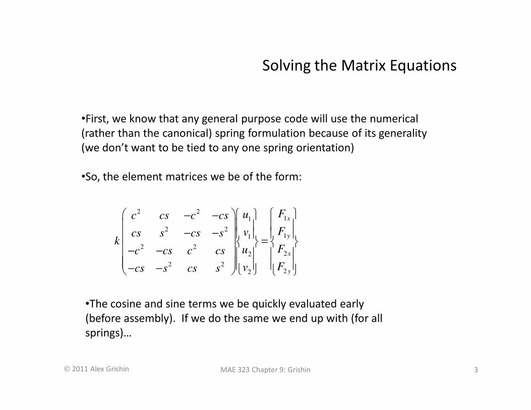
•First, we know that any general purpose code will use the numerical

(rather than the canonical) spring formulation because of its generality

(we don’t want to be tied to any one spring orientation)

•So, the element matrices we be of the form:

2 211

2 211

2 222

2 222

x

y

x

y

Fuc cs c cs

Fvcs s cs sk

Fuc cs c cs

Fvcs s cs s

− −

− − = − − − −

•The cosine and sine terms we be quickly evaluated early

(before assembly). If we do the same we end up with (for all

springs)…



11

11

22

22

0 0 0 0

0 1 0 1

0 0 0 0

0 1 0 1

x

y

x

y

Fu

Fvk

Fu

Fv

− = −

x

y

u1

u2

u3,F3

k2

k1

k3

2

3

4

1

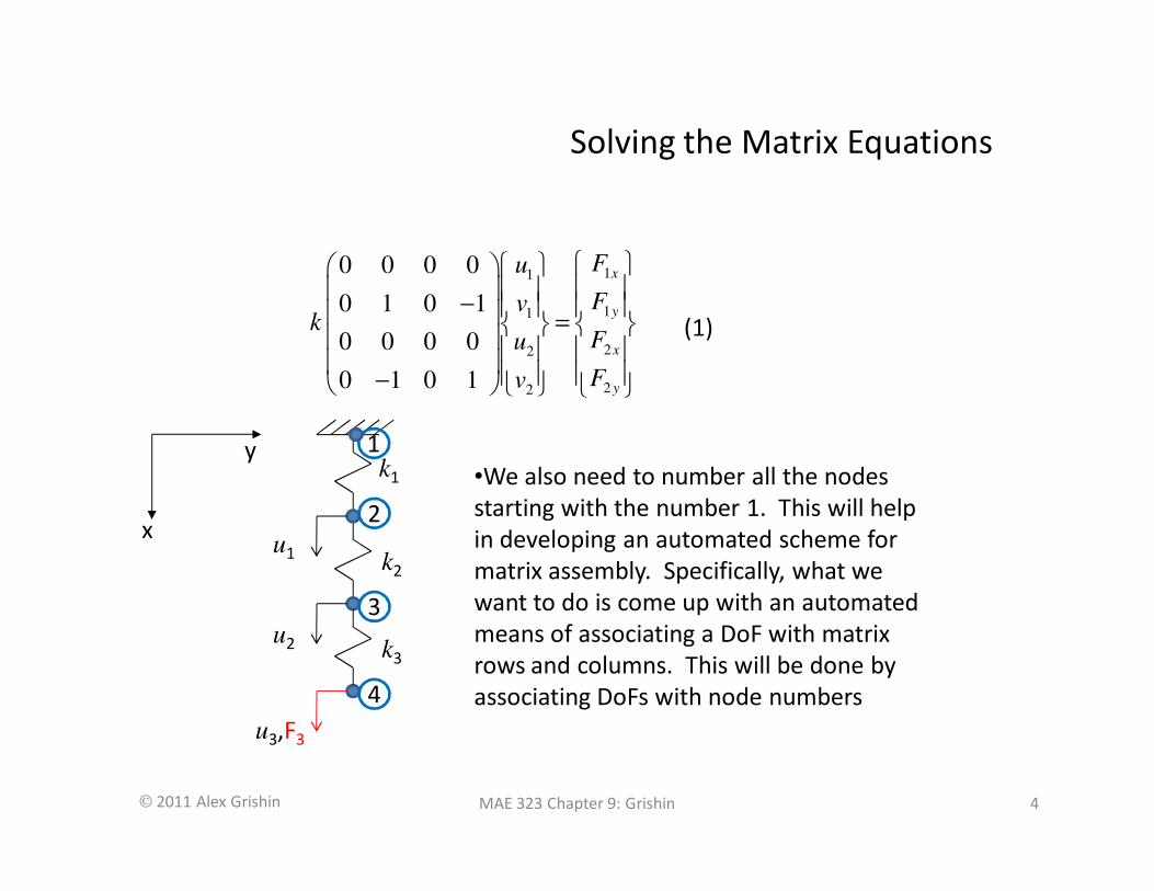
•We also need to number all the nodes

starting with the number 1. This will help

in developing an automated scheme for

matrix assembly. Specifically, what we

want to do is come up with an automated

means of associating a DoF with matrix

rows and columns. This will be done by

associating DoFs with node numbers

(1)



•A simple and common way to assocate DoFs with node

numbers is to number them with a scheme such as:

# * , { | ,0 }DoF n i q q q q q n= − = ∈ ≤ ≤ℕ

where i is the node number, n is the number of DoFs per node,

and q is an integer than ranges between 0 and n (inclusive)

•Thus, for example, element 1 (k1) with nodes 1 and 2, would receive the

following DoF indices (third column below):

element # node # q n DoF # (n*i-q) description

1 1 1 2 1 ux1

1 1 0 2 2 uy1

1 2 1 2 3 ux2

1 2 0 2 4 uy2



•And, similarly for elements 2 and 3:


3 3 1 2 5 Ux3

3 3 0 2 6 Uy3

3 4 1 2 7 Ux4

3 4 0 2 8 uy4


2 2 1 2 3 Ux2

2 2 0 2 4 Uy2

2 3 1 2 5 Ux3

2 3 0 2 6 uy3

•Notice the last DoF number (8) corresponds with the size of the

assembled matrix (which we already knew thanks to our

estimate of number of nodes x number of DoFs per node):



•We now have everything we need to assemble the global stiffness

matrix and applied load vector (the system equations). Recall from

Chapter 2 that the Direct Stiffness Method (DSM) gives us the assembly

algorithm:

1

1

N

n

n

N

n

n

=

=

=

=

∑

∑

K k

F f

Where K and F are the assembled stiffness matrix and force vector,

respectively, and kn and fn are the element stiffness matrix and force

vector for element n in the global reference frame (this last part is

important).

•And the global matrix indices for each element (and associated load

vector) are given by the three tables we saw previously

(2)



•So, to keep things simple, lets assume that the k1=k2=k3=k. We can re-

rewrite (1) using the global indices:

1

2

1 1 1

3

4

0 0 0 0 0

0 1 0 1 0

0 0 0 0 0

0 1 0 1 0

u

uk

u

u

− = = = −

k u f

Similarly, for the other elements:

3

4

2 2 2

5

6

0 0 0 0 0

0 1 0 1 0

0 0 0 0 0

0 1 0 1 0

u

uk

u

u

− = = = −

k u f

5

6

3 3 3

7

8

0 0 0 0 0

0 1 0 1 0

0 0 0 0 0

0 1 0 1

u

uk

u

u F

− = = = −

k u f

(3)

(4)

(5)



•The global matrix equation is assembled by first initializing

an 8 x 8 matrix and an 8 x 1 vector for K and F respectively.

Then equation (2) is applied using (3), (4), and (5) to yield:

1

2

3

4

5

6

7

8

0 0 0 0 0 0 0 0 0

0 1 0 1 0 0 0 0 0

0 0 0 0 0 0 0 0 0

0 1 0 2 0 1 0 0 0

0 0 0 0 0 0 0 0 0

0 0 0 1 0 2 0 1 0

0 0 0 0 0 0 0 0 0

0 0 0 0 1 0 0 1

u

u

u

uk

u

u

u

u F

−

− − =

− − −

•But now we have a problem. What to do about the zeros on the

diagonal? These correspond to the fact that the springs have no stiffness

in the x-direction. Although we don’t have any loads in the x-direction,

we still have a singular system. If we were solving this system by hand,

we might simply eliminate the rows and columns with zeros in them.

However, this is not a robust programming solution

(6)



•A simpler programming approach (which allows us to keep the same

matrix size throughout) would be to use the “zero-one rule”. This

rule operates as follows. For each prescribed DoF, uJ:

1. Subtract KiJ⋅uJ from the RHS

2. Set entries on row J equal to zero

3. Set the diagonal member on row J (JJ) equal to 1 and set

FJ=uJ

*This is a common solution. Note, however that a complication arises if there are forces in the x-

direction. Typical solutions to this complication can yield misleading results

1

2

3

4

5

6

7

8

1/ 0 0 0 0 0 0 0 0

0 1/ 0 0 0 0 0 0 0

0 0 1/ 0 0 0 0 0 0

0 0 0 2 0 1 0 0 0

0 0 0 0 1/ 0 0 0 0

0 0 0 1 0 2 0 1 0

0 0 0 0 0 0 1/ 0 0

0 0 0 0 1 0 0 1

uk

uk

uk

uk

uk

u

uk

u F

− =

− − −

•Application of these rules to u2 , but also all x DoFs yields:

(7)



•Solution of (7) yields: 0

0

0

/

0

2 /

0

3 /

F k

F k

F k

=

u

•Which we immediately recognize to be the correct solution

•Now, we have applied the zero-one rule, not only to the applied zero y-

displacement at node 1 (u2), but also to all the DoFs in the x-direction. We

have done this because:

•We know we don’t have DoFs in the x-direction (so setting them equal to

zero shouldn’t hurt anything. For exceptions, see the footnote on the

previous slide). We’ll revisit this concept later

•We can’t solve the system otherwise



•Equation (7) reveals another important property of finite element equations –

Namely, that they result in “sparse” systems. A sparse matrix is one which is

made mostly of zeroes. Another helpful feature of finite element equations is

that they tend to be “banded”, meaning that the majority of nonzero terms

cluster around the main diagonal (or can be made to do so). This feature greatly

reduces solution times in “direct” solvers. We will spend some time explaining

these concepts in more detail.

•An official definition of “bandwidth” is* the following: For a square banded

matrix A=aij, all matrix elements are zero outside a diagonally bordered band

whose range is given by constants k1 and k2. More formally:

* http://en.wikipedia.org/wiki/Matrix_bandwidth

1 2 1 20 if or , where , 0ija j i k j i k k k= < − > + ≥

•The quantities k1 and k2 are called the left and right half-bandwidth.

The matrix bandwidth is k1+k2+1



•In other words, the bandwidth is the smallest number of adjacent

diagonals to which all nonzero elements are confined. Clearly, as the

bandwidth approaches the matrix size, the matrix is no longer considered

“banded”..

•Some examples: The K matrix of equation (7) has a half bandwidth of 2

and a bandwidth of 5. it is sometimes helpful to plot such matrices as a

grid with nonzero entries represented as colored cells, and each cell of

the grid representing a matrix element (symbolic math software tends to

come with such functionality. We’re using Mathematica). The stiffness

matrix of (7) looks like this when plotted in this way:

•We’ll call such a

plot “the

sparsity pattern”

of the matrix



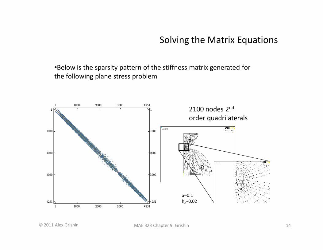
•Below is the sparsity pattern of the stiffness matrix generated for

the following plane stress problem

a

a∼0.1

hc∼0.02

Ω1

Ω2

2100 nodes 2nd

order quadrilaterals



•Hopefully, the student can now see the value of sparse matrices. Consider

the case shown in the previous slide, for example. This matrix is 4251 x

4251. Now, if the computer is using double-precision arithmetic, each

element of the matrix would get stored as a floating point number consisting

of 8 bytes of memory*. This results in 4251 x 4251 x 8 bytes, or

approximately 144 Mbytes of storage.

•One can see that this quickly gets out of hand, as the storage requirement

grows in proportion to the square of the matrix size. For example, if the

matrix size were increased by a factor of 10, the storage requirement would

grow to approximately 14 Gbyte! In this case, a factor of 10 increase in

matrix size corresponds to only a factor of 5 increase in model size (node

count). In other words, a 10,000 node model would push the current limits

on personal computing!

*on 64-bit machines using the IEEE 754 standard



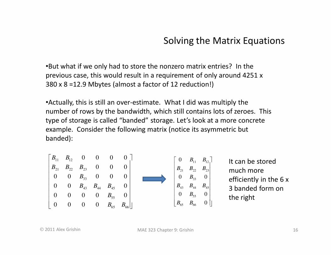
•But what if we only had to store the nonzero matrix entries? In the

previous case, this would result in a requirement of only around 4251 x

380 x 8 =12.9 Mbytes (almost a factor of 12 reduction!)

•Actually, this is still an over-estimate. What I did was multiply the

number of rows by the bandwidth, which still contains lots of zeroes. This

type of storage is called “banded” storage. Let’s look at a more concrete

example. Consider the following matrix (notice its asymmetric but

banded):

11 12

21 22 23

33

43 44 45

55

65 66

0 0 0 0

0 0 0

0 0 0 0 0

0 0 0

0 0 0 0 0

0 0 0 0

B B

B B B

B

B B B

B

B B

11 12

21 22 23

33

43 44 45

55

65 66

0

0 0

0 0

0

B B

B B B

B

B B B

B

B B

It can be stored

much more

efficiently in the 6 x

3 banded form on

the right



•So, banded storage certainly helps. But one can see there’s still room for

improvement. In the previous example, we managed to reduce the storage

requirement for a 6 x 6 down to a 6 x 3. But this is still 50 percent larger

than the number of nonzero entries (12).

•So , we can see that, to the extent that not all banded matrices are

“perfectly” banded (that is to say: still contain zeroes within their bands),

and not all sparse matrices will be banded (for example, adding constraints

tends to destroy bandedness), a more robust storage mechanism is

required. Such storage mechanisms are usually referred to as “sparse”

•Solvers can be modified to operate on matrices stored in banded format

without too much effort (both Cholesky and LU deocomposition methods,

for example, can be easily modified to accommodate the banded format).

Such banded storage schemes and solvers dominated much finite element

code from the late 70’s into the early 90’s



•Sparse matrix storage involves storing the nonzero terms of a matrix

in a vector. The row and column indices of each entry are stored in

separate vectors. Several competing methods exist which are beyond

the scope of this course. It is important, however, to know whether a

particular linear solver operates on matrices stored in a sparse

format or not.

•Because such solvers are relatively new to the marketplace

(beginning in the 90’s), not all commercial codes may utilize sparse

matrix solvers or formats



Matrix Solvers



•There are basically two types of matrix solvers. We might call these

“direct” and “iterative”. Direct matrix solvers use some variant of the

Gaussian elimination procedure, while iterative solvers start with an

solution vector “guess”, and then iterate until a residual is smaller

than some threshold value.

•Depending on the software either or both of these methods might

be available. Typically either or both will support either banded or

sparse matrix formats.



Direct Methods

•Most direct methods use a factorization scheme (decomposition*) with back

substitution**. What these means in practice is that, in order to be successful:

•The system equations must be easily factorable (positive definite, for

example)

•You must have enough computer resources (usually RAM) in order to

perform this costly step

•The model must be fully constrained and not have material

properties which vary greatly (Ratios of Young’s modulus, for

example, that exceed values of around 1,000)

•The last requirement is rather important. When material properties are vastly

different, the matrix behaves as though the model is not properly constrained.

Most solvers catch this during the “pivot” operation, in which they attempt to

perform row or column operations to maximize the absolute value of numbers

on the diagonal. This operation is important for stability and accuracy

see: http://en.wikipedia.org/wiki/Matrix_factorization

**: http://en.wikipedia.org/wiki/Back_substitution#Forward_and_back_substitution



Direct Methods

•We should mention here that some codes offer another variant of the direct

method, which uses a Gaussian procedure to incrementally solve the model

AS the matrices are being assembled! Such solvers are called “frontal” or

“wavefront” solvers (this option is still available in ANSYS Mechanical APDL)

•The number of equations which are active after any element has been

processed is called the “wavefront” at that time. The maximum size of this

wavefront can be controlled. This is very beneficial when one has limited

available RAM (this is why the procedure was once quite popular –it dates to a

time when such memory was only available on the CPU itself – and then only

at a fraction of what is available today)

•The total number of operations performed with this method, while still vastly

smaller than if one solved the full (unbanded) system at once, is still greater

than that achieved in sparse solvers. Again, the main benefit here is when

available RAM is severely limited (as might be the case with an old computer)



Iterative Methods

•If a matrix fails to obey any or all of the previous requirements of direct solvers,

it may be beneficial to use an iterative technique. Most modern commercial

codes will have at least one such method available, which will operate either on

a banded or sparse matrix format. The most popular and general method

available today is the Conjugate Gradient Method (of which there many variants.

This is the default solver you get when you choose an iterative solver in

Workbench). Benefits of iterative methods are:

•They tend to use less RAM than direct methods for the same problem

size

•They can still converge to reasonable solutions even when the

matrices are ill-conditioned, as can occur when the model is either

improperly constrained, or has considerably dissimilar material

properties

•Their performance is far less dependent on matrix properties such as

symmetry. This makes them well-suited for nonlinear tasks such as

contact with friction and fluid/structure interaction



Solving Structural

Problems in ANSYS



•From the ANSYS 13.0 documentation (March, 2011. Performance Guide), we

learn the following very important facts:

•The amount of memory needed to assemble a matrix entirely

within available RAM is approximately 1 Gbyte per million DoFs

•The amount of memory needed to hold the factored matrix in

memory is approximately 10 to 20 Gbyte per million DoFs

•The second bullet above is more relevant to our discussion. It means

that if you want to use the direct solver (the default in Workbench), and

you have a model with one million DoFs (not uncommon today), you

need anywhere from 10 to Gbyte of RAM if you want to solve entirely

within available RAM!



•The factor of 10-20 to 1 (factored matrix to assembled sparse matrix) is

a direct result of the fact that decomposed triangular matrices (which is

what the factorization routine tries to achieve) are necessarily dense,

even if the parent matrix was very sparse!

•This represents a significant obstacle to the efficient solving of sparse

systems. ANSYS offers their own rather unique solution to this

restriction with an “out-of-core” solution capability. This is a

proprietary means of solving the factored matrix incrementally by

reading and writing pieces of it to the disk drive sequentially

•When this happens, the user is informed through the output window

(Solution Information in Workbench) that an out-of-core solution is

taking place. The user is also told how much RAM is required for a

complete in-core solution



•By contrast the iterative family of solvers have the

following basic system requirements:

•Base amount of availabe RAM: 1 Gbyte per

Million DoFs

•Basic I/O requirement (disk read/write): 1.5

Gbyte per Million DoFs

•So one sees that the iterative solver is potentially much more efficient for

large problems. Although a precise prediction of the performance can get

rather complicated, it is the instructor’s experience (and that of PADT

generally) that the PCG solver usually produces the fastest results. In

addition, we have found it to be superior in handling systems with many

constraints. Students should beware, however, that this directly contradicts

the ANSYS documentation

matrix assembly in fea - padtinc.com

Documents