matrices: theory and applications - 213.230.96.51:8090
TRANSCRIPT

Matrices:Theory and Applications
Denis Serre
Springer

Graduate Texts in Mathematics 216Editorial Board
S. Axler F.W. Gehring K.A. Ribet

This page intentionally left blank

Denis Serre
MatricesTheory and Applications

Denis SerreEcole Normale Superieure de LyonUMPALyon Cedex 07, [email protected]
Editorial Board:S. Axler F.W. Gehring K.A. RibetMathematics Department Mathematics Department Mathematics DepartmentSan Francisco State East Hall University of California,
University University of Michigan BerkeleySan Francisco, CA 94132 Ann Arbor, MI 48109 Berkeley, CA 94720-3840USA USA [email protected] [email protected] [email protected]
Mathematics Subject Classification (2000): 15-01
Library of Congress Cataloging-in-Publication DataSerre, D. (Denis)
[Matrices. English.]Matrices : theory and applications / Denis Serre.
p. cm.—(Graduate texts in mathematics ; 216)Includes bibliographical references and index.ISBN 0-387-95460-0 (alk. paper)1. Matrices I. Title. II. Series.
QA188 .S4713 2002512.9′434—dc21 2002022926
ISBN 0-387-95460-0 Printed on acid-free paper.
Translated from Les Matrices: Theorie et pratique, published by Dunod (Paris), 2001.
2002 Springer-Verlag New York, Inc.All rights reserved. This work may not be translated or copied in whole or in part without thewritten permission of the publisher (Springer-Verlag New York, Inc., 175 Fifth Avenue, New York,NY 10010, USA), except for brief excerpts in connection with reviews or scholarly analysis. Usein connection with any form of information storage and retrieval, electronic adaptation, computersoftware, or by similar or dissimilar methodology now known or hereafter developed is forbidden.The use in this publication of trade names, trademarks, service marks, and similar terms, even ifthey are not identified as such, is not to be taken as an expression of opinion as to whether or notthey are subject to proprietary rights.
Printed in the United States of America.
9 8 7 6 5 4 3 2 1 SPIN 10869456
Typesetting: Pages created by the author in LaTeX2e.
www.springer-ny.com
Springer-Verlag New York Berlin HeidelbergA member of BertelsmannSpringer Science+Business Media GmbH

To Pascale and Joachim

This page intentionally left blank

Preface
The study of matrices occupies a singular place within mathematics. Itis still an area of active research, and it is used by every mathematicianand by many scientists working in various specialities. Several examplesillustrate its versatility:
• Scientific computing libraries began growing around matrix calculus.As a matter of fact, the discretization of partial differential operatorsis an endless source of linear finite-dimensional problems.
• At a discrete level, the maximum principle is related to nonnegativematrices.
• Control theory and stabilization of systems with finitely many degreesof freedom involve spectral analysis of matrices.
• The discrete Fourier transform, including the fast Fourier transform,makes use of Toeplitz matrices.
• Statistics is widely based on correlation matrices.
• The generalized inverse is involved in least-squares approximation.
• Symmetric matrices are inertia, deformation, or viscous tensors incontinuum mechanics.
• Markov processes involve stochastic or bistochastic matrices.
• Graphs can be described in a useful way by square matrices.

viii Preface
• Quantum chemistry is intimately related to matrix groups and theirrepresentations.
• The case of quantum mechanics is especially interesting: Observablesare Hermitian operators, their eigenvalues are energy levels. In theearly years, quantum mechanics was called “mechanics of matrices,”and it has now given rise to the development of the theory of largerandom matrices. See [23] for a thorough account of this fashionabletopic.
This text was conceived during the years 1998–2001, on the occasion ofa course that I taught at the Ecole Normale Superieure de Lyon. As such,every result is accompanied by a detailed proof. During this course I triedto investigate all the principal mathematical aspects of matrices: algebraic,geometric, and analytic.
In some sense, this is not a specialized book. For instance, it is not asdetailed as [19] concerning numerics, or as [35] on eigenvalue problems,or as [21] about Weyl-type inequalities. But it covers, at a slightly higherthan basic level, all these aspects, and is therefore well suited for a gradu-ate program. Students attracted by more advanced material will find oneor two deeper results in each chapter but the first one, given with fullproofs. They will also find further information in about the half of the170 exercises. The solutions for exercises are available on the author’s sitehttp://www.umpa.ens-lyon.fr/ ˜serre/exercises.pdf.
This book is organized into ten chapters. The first three contain thebasics of matrix theory and should be known by almost every graduatestudent in any mathematical field. The other parts can be read more orless independently of each other. However, exercises in a given chaptersometimes refer to the material introduced in another one.
This text was first published in French by Masson (Paris) in 2000, underthe title Les Matrices: theorie et pratique. I have taken the opportunityduring the translation process to correct typos and errors, to index a listof symbols, to rewrite some unclear paragraphs, and to add a modestamount of material and exercises. In particular, I added three sections,concerning alternate matrices, the singular value decomposition, and theMoore–Penrose generalized inverse. Therefore, this edition differs from theFrench one by about 10 percent of the contents.
Acknowledgments. Many thanks to the Ecole Normale Superieure de Lyonand to my colleagues who have had to put up with my talking to themso often about matrices. Special thanks to Sylvie Benzoni for her constantinterest and useful comments.
Lyon, France Denis SerreDecember 2001

Contents
Preface vii
List of Symbols xiii
1 Elementary Theory 11.1 Basics . . . . . . . . . . . . . . . . . . . . . . . . . . . . 11.2 Change of Basis . . . . . . . . . . . . . . . . . . . . . . . 81.3 Exercises . . . . . . . . . . . . . . . . . . . . . . . . . . . 13
2 Square Matrices 152.1 Determinants and Minors . . . . . . . . . . . . . . . . . . 152.2 Invertibility . . . . . . . . . . . . . . . . . . . . . . . . . 192.3 Alternate Matrices and the Pfaffian . . . . . . . . . . . . 212.4 Eigenvalues and Eigenvectors . . . . . . . . . . . . . . . 232.5 The Characteristic Polynomial . . . . . . . . . . . . . . . 242.6 Diagonalization . . . . . . . . . . . . . . . . . . . . . . . 282.7 Trigonalization . . . . . . . . . . . . . . . . . . . . . . . . 292.8 Irreducibility . . . . . . . . . . . . . . . . . . . . . . . . . 302.9 Exercises . . . . . . . . . . . . . . . . . . . . . . . . . . . 31
3 Matrices with Real or Complex Entries 403.1 Eigenvalues of Real- and Complex-Valued Matrices . . . 433.2 Spectral Decomposition of Normal Matrices . . . . . . . 453.3 Normal and Symmetric Real-Valued Matrices . . . . . . 47

x Contents
3.4 The Spectrum and the Diagonal of Hermitian Matrices . 513.5 Exercises . . . . . . . . . . . . . . . . . . . . . . . . . . . 55
4 Norms 614.1 A Brief Review . . . . . . . . . . . . . . . . . . . . . . . 614.2 Householder’s Theorem . . . . . . . . . . . . . . . . . . . 664.3 An Interpolation Inequality . . . . . . . . . . . . . . . . 674.4 A Lemma about Banach Algebras . . . . . . . . . . . . . 704.5 The Gershgorin Domain . . . . . . . . . . . . . . . . . . 714.6 Exercises . . . . . . . . . . . . . . . . . . . . . . . . . . . 73
5 Nonnegative Matrices 805.1 Nonnegative Vectors and Matrices . . . . . . . . . . . . . 805.2 The Perron–Frobenius Theorem: Weak Form . . . . . . . 815.3 The Perron–Frobenius Theorem: Strong Form . . . . . . 825.4 Cyclic Matrices . . . . . . . . . . . . . . . . . . . . . . . 855.5 Stochastic Matrices . . . . . . . . . . . . . . . . . . . . . 875.6 Exercises . . . . . . . . . . . . . . . . . . . . . . . . . . . 91
6 Matrices with Entries in a Principal Ideal Domain;Jordan Reduction 976.1 Rings, Principal Ideal Domains . . . . . . . . . . . . . . 976.2 Invariant Factors of a Matrix . . . . . . . . . . . . . . . . 1016.3 Similarity Invariants and Jordan Reduction . . . . . . . 1046.4 Exercises . . . . . . . . . . . . . . . . . . . . . . . . . . . 111
7 Exponential of a Matrix, Polar Decomposition, andClassical Groups 1147.1 The Polar Decomposition . . . . . . . . . . . . . . . . . . 1147.2 Exponential of a Matrix . . . . . . . . . . . . . . . . . . 1167.3 Structure of Classical Groups . . . . . . . . . . . . . . . 1207.4 The Groups U(p, q) . . . . . . . . . . . . . . . . . . . . . 1227.5 The Orthogonal Groups O(p, q) . . . . . . . . . . . . . . 1237.6 The Symplectic Group Spn . . . . . . . . . . . . . . . . 1277.7 Singular Value Decomposition . . . . . . . . . . . . . . . 1287.8 Exercises . . . . . . . . . . . . . . . . . . . . . . . . . . . 130
8 Matrix Factorizations 1368.1 The LU Factorization . . . . . . . . . . . . . . . . . . . . 1378.2 Choleski Factorization . . . . . . . . . . . . . . . . . . . 1428.3 The QR Factorization . . . . . . . . . . . . . . . . . . . . 1438.4 The Moore–Penrose Generalized Inverse . . . . . . . . . 1458.5 Exercises . . . . . . . . . . . . . . . . . . . . . . . . . . . 147
9 Iterative Methods for Linear Problems 149

Contents xi
9.1 A Convergence Criterion . . . . . . . . . . . . . . . . . . 1509.2 Basic Methods . . . . . . . . . . . . . . . . . . . . . . . . 1519.3 Two Cases of Convergence . . . . . . . . . . . . . . . . . 1539.4 The Tridiagonal Case . . . . . . . . . . . . . . . . . . . . 1559.5 The Method of the Conjugate Gradient . . . . . . . . . . 1599.6 Exercises . . . . . . . . . . . . . . . . . . . . . . . . . . . 165
10 Approximation of Eigenvalues 16810.1 Hessenberg Matrices . . . . . . . . . . . . . . . . . . . . 16910.2 The QR Method . . . . . . . . . . . . . . . . . . . . . . . 17310.3 The Jacobi Method . . . . . . . . . . . . . . . . . . . . . 18010.4 The Power Methods . . . . . . . . . . . . . . . . . . . . . 18410.5 Leverrier’s Method . . . . . . . . . . . . . . . . . . . . . 18810.6 Exercises . . . . . . . . . . . . . . . . . . . . . . . . . . . 190
References 195
Index 199

This page intentionally left blank

List of Symbols
|A|, 80a|b, 97A B, 59A†, 145A ≥ 0, 80a ≺ b, 52a ∼ b, 97A∗, 15, 97
B ⊗ C, 13(b), 97BP , 106
Cn, 33Cr, 83
∆n, 87δj
i , 5detM , 16Di, 71diag(d1, . . . , dn), 5dim E, 3dimK F , 3Dk(N), 102
e, 87ei, 3
EK(λ), 28Eλ, 29End(E), 7ε(σ), 16exp A, 116
F + G, 2F ⊕ G, 3F ⊕⊥ G, 12F⊥, 11
G, 152G, 121G(A), 71Gα, 125GCC , 3gcd, 98GLn(A), 20G0, 126
H ≥ h, 42H ≥ 0n, 42Hn, 41HPDn, 42√
H , 115
, imaginary part, 56

xiv List of Symbols
In, 5
J , 151J(a; r), 110Jik, 100J2, 132J3, 132J4, 132
K(A), 162K, 4kerM , 7keru, 7KI , 2K(M), 6Kn, 57K[X], 15k[X, Y ], 99
λk(A), 57L(E,F ), 7Lω, 152
adjM , 17M , 40M , 17
M
(i1 i2 · · · ipj1 j2 · · · jp
), 17
Mk, 6M−1, 20M−k, 20M−T , 20[M, N ], 6Mn(K), 5Mn×m(K), 5M∗, 40M−∗, 40MT , 10
‖ A ‖, 64‖ A ‖p, 65‖ x ‖p, 61‖ x ‖A, 154‖ x ‖∞, 61‖ · ‖′, 64||| · |||, 65
ωJ , 1580n, 5
On(K), 200nm, 5O−
n , 123O(p, q), 120⊥A, 160
Pf, 22PG, 156π0, 125PJ , 156PM , 24Pω, 156p′, 62PSL2(IR), 56
RA(F ), 57rk M , 5, real part, 63R(h; A), 92ρ(A), 61R(M), 8r(x), 70, 160
〈x, y〉, 11, 41S∆n, 90σr, 188sj(A), 75sk(a), 52SLn(A), 20sm, 189Sn, 15SOn(K), 20S1, 86Sp(M), 24SpK(M), 24SPDn, 42Spm, 120Spm, 120S2, 56, 126SUn, 41Symn(K), 10
τ , 151τCG, 164Tk, 162Tr M , 25
Un, 41Up, 85

List of Symbols xv
U(p, q), 120u∗, 42uT , 11
V (a), 173
|x|, 80x ≤ y, 80x > 0, 80x ≥ 0, 80

This page intentionally left blank

1Elementary Theory
1.1 Basics
1.1.1 Vectors and Scalars
Fields. Let (K, +, ·) be a field. It could be IR, the field of real numbers, CC(complex numbers), or, more rarely, QQ (rational numbers). Other choicesare possible, of course. The elements of K are called scalars.
Given a field k, one may build larger fields containing k: algebraic ex-tensions k(α1, . . . , αn), fields of rational fractions k(X1, . . . , Xn), fields offormal power series k[[X1, . . . , Xn]]. Since they are rarely used in this book,we do not define them and let the reader consult his or her favorite textbookon abstract algebra.
The digits 0 and 1 have the usual meaning in a field K, with 0 + x =1 · x = x. Let us consider the subring ZZ1, composed of all sums (possiblyempty) of the form ±(1 + · · ·+ 1). Then ZZ1 is isomorphic to either ZZ orto a field ZZ/pZZ. In the latter case, p is a prime number, and we call it thecharacteristic of K. In the former case, K is said to have characteristic 0.
Vector spaces. Let (E, +) be a commutative group. Since E is usuallynot a subset of K, it is an abuse of notation that we use + for the additivelaws of both E and K. Finally, let
(a, x) → ax,
K × E → E,

2 1. Elementary Theory
be a map such that
(a + b)x = ax + bx, a(x + y) = ax + ay.
One says that E is a vector space over K (one often speaks of a K-vectorspace) if moreover,
a(bx) = (ab)x, 1x = x,
hold for all a, b ∈ K and x ∈ E. The elements of E are called vectors. In avector space one always has 0x = 0 (more precisely, 0Kx = 0E).
When P, Q ⊂ K and F, G ⊂ E, one denotes by PQ (respectively P +Q, F+G, PF ) the set of products pq as (p, q) ranges over P×Q (respectivelyp+q, f+g, pf as p, q, f, g range over P, Q, F, G). A subgroup (F, +) of (E, +)that is stable under multiplication by scalars, i.e., such that KF ⊂ F , isagain a K-vector space. One says that it is a linear subspace of E, or just asubspace. Observe that F , as a subgroup, is nonempty, since it contains 0E .The intersection of any family of linear subspaces is a linear subspace. Thesum F + G of two linear subspaces is again a linear subspace. The trivialformula (F + G) + H = F + (G + H) allows us to define unambiguouslyF + G+ H and, by induction, the sum of any finite family of subsets of E.When these subsets are linear subspaces, their sum is also a linear subspace.
Let I be a set. One denotes by KI the set of maps a = (ai)i∈I : I → Kwhere only finitely many of the ai’s are nonzero. This set is naturallyendowed with a K-vector space structure, by the addition and productlaws
(a + b)i := ai + bi, (λa)i := λai.
Let E be a vector space and let i → fi be a map from I to E. A linearcombination of (fi)i∈I is a sum ∑
i∈I
aifi,
where the ai’s are scalars, only finitely many of which are nonzero (in otherwords, (ai)i∈I ∈ KI). This sum involves only finitely many terms. It is avector of E. The family (fi)i∈I is free if every linear combination but thetrivial one (when all coefficients are zero) is nonzero. It is a generatingfamily if every vector of E is a linear combination of its elements. In otherwords, (fi)i∈I is free (respectively generating) if the map
KI → E,
(ai)i∈I →∑i∈I
aifi,
is injective (respectively onto). Last, one says that (fi)i∈I is a basis of E ifit is free and generating. In that case, the above map is bijective, and it isactually an isomorphism between vector spaces.

1.1. Basics 3
If G ⊂ E, one often identifies G and the associated family (g)g∈G . The setG of linear combinations of elements of G is a linear subspace E, called thelinear subspace spanned by G. It is the smallest linear subspace E containingG, equal to the intersection of all linear subspaces containing G. The subsetG is generating when G = E.
One can prove that every K-vector space admits at least one basis. Inthe most general setting, this is a consequence of the axiom of choice.All the bases of E have the same cardinality, which is therefore called thedimension of E, denoted by dimE. The dimension is an upper (respectivelya lower) bound for the cardinality of free (respectively generating) families.In this book we shall only use finite-dimensional vector spaces. If F, G aretwo linear subspaces of E, the following formula holds:
dim F + dimG = dimF ∩G + dim(F + G).
If F ∩ G = 0, one writes F ⊕ G instead of F + G, and one says that Fand G are in direct sum. One has then
dimF ⊕G = dim F + dimG.
Given a set I, the family (ei)i∈I , defined by
(ei)j =
0, j = i,1, j = i,
is a basis of KI , called the canonical basis. The dimension of KI is thereforeequal to the cardinality of I.
In a vector space, every generating family contains at least one basis ofE. Similarly, given a free family, it is contained in at least one basis of E.This is the incomplete basis theorem.
Let L be a field and K a subfield of L. If F is an L-vector space, then Fis also a K-vector space. As a matter of fact, L is itself a K-vector space,and one has
dimK F = dimL F · dimK L.
The most common example (the only one that we shall consider) is K = IR,L = CC, for which we have
dimIR F = 2 dimCC F.
Conversely, if G is an IR-vector space, one builds its complexification GCC
as follows:
GCC = G×G,
with the induced structure of an additive group. An element (x, y) of GCC
is also denoted x + iy. One defines multiplication by a complex number by
(λ = a + ib, z = x + iy) → λz := (ax− by, ay + bx).

4 1. Elementary Theory
One verifies easily that GCC is a CC-vector space, with
dimCC GCC = dimIR G.
Furthermore, G may be identified with an IR-linear subspace of GCC by
x → (x, 0).
Under this identification, one has GCC = G+ iG. In a more general setting,one may consider two fields K and L with K ⊂ L, instead of IR and CC, butthe construction of GL is more delicate and involves the notion of tensorproduct. We shall not use it in this book.
One says that a polynomial P ∈ L[X ] splits over L if it can be writtenas a product of the form
a
r∏i=1
(X − ai)ni , a, ai ∈ L, r ∈ IN, ni ∈ IN ∗.
Such a factorization is unique, up to the order of the factors. A field L inwhich every nonconstant polynomial P ∈ L[X ] admits a root, or equiva-lently in which every polynomial P ∈ L[X ] splits, is algebraically closed. Ifthe field K ′ contains the field K and if every polynomial P ∈ K[X ] admitsa root in K ′, then the set of roots in K ′ of polynomials in K[X ] is an alge-braically closed field that contains K, and it is the smallest such field. Onecalls K ′ the algebraic closure of K. Every field K admits an algebraic clo-sure, unique up to isomorphism, denoted by K. The fundamental theoremof algebra asserts that IR = CC. The algebraic closure of QQ, for instance,is the set of algebraic complex numbers, meaning that they are roots ofpolynomials P ∈ ZZ[X ].
1.1.2 Matrices
Let K be a field. If n, m ≥ 1, a matrix of size n×m with entries in K is amap from 1, . . . , n × 1, . . . , m with values in K. One represents it asan array with n rows and m columns, an element of K (an entry) at eachpoint of intersection of a row an a column. In general, if M is the name ofthe matrix, one denotes by mij the element at the intersection of the ithrow and the jth column. One has therefore
M =
m11 . . . m1m
.... . .
...mn1 . . . mnm
,
which one also writes
M = (mij)1≤i≤n,1≤j≤m.
In particular circumstances (extraction of matrices or minors, for example)the rows and the columns can be numbered in a different way, using non-

1.1. Basics 5
consecutive numbers. One needs only two finite sets, one for indexing therows, the other for indexing the columns.
The set of matrices of size n × m with entries in K is denoted byMn×m(K). It is an additive group, where M + M ′ denotes the matrix M ′′
whose entries are given by m′′ij = mij + m′
ij . One defines likewise multipli-cation by a scalar a ∈ K. The matrix M ′ := aM is defined by m′
ij = amij .One has the formulas a(bM) = (ab)M , a(M + M ′) = (aM) + (aM ′), and(a + b)M = (aM) + (bM), which endow Mn×m(K) with a K-vector spacestructure. The zero matrix is denoted by 0, or 0nm when one needs to avoidambiguity.
When m = n, one writes simply Mn(K) instead of Mn×n(K), and 0n
instead of 0nn. The matrices of sizes n× n are called square matrices. Onewrites In for the identity matrix, defined by
mij = δji =
0, if i = j,1, if i = j.
In other words,
In =
1 0 · · · 0
0. . . . . .
......
. . . . . . 00 · · · 0 1
.
The identity matrix is a special case of a permutation matrix, which aresquare matrices having exactly one nonzero entry in each row and eachcolumn, that entry being a 1. In other words, a permutation matrix Mreads
mij = δσ(j)i
for some permutation σ ∈ Sn.A square matrix for which i < j implies mij = 0 is called a lower
triangular matrix. It is upper triangular if i > j implies mij = 0. It isstrictly upper triangular if i ≥ j implies mij = 0. Last, it is diagonal if mij
vanishes for every pair (i, j) such that i = j. In particular, given n scalarsd1, . . . , dn ∈ K, one denotes by diag(d1, . . . , dn) the diagonal matrix whosediagonal term mii equals di for every index i.
When m = 1, a matrix M of size n × 1 is called a column vector. Oneidentifies it with the vector of Kn whose ith coordinate in the canonicalbasis is mi1. This identification is an isomorphism between Mn×1(K) andKn. Likewise, the matrices of size 1×m are called row vectors.
A matrix M ∈ Mn×m(K) may be viewed as the ordered list of itscolumns M (j) (1 ≤ j ≤ m). The dimension of the linear subspace spannedby the M (j) in Kn is called the rank of M and denoted by rk M .

6 1. Elementary Theory
1.1.3 Product of Matrices
Let n, m, p ≥ 1 be three positive integers. We define a (noncommutative)multiplication law
Mn×m(K)×Mm×p(K) → Mn×p(K),(M, M ′) → MM ′,
which we call the product of M and M ′. The matrix M ′′ = MM ′ is givenby the formula
m′′ij =
m∑k=1
mikm′kj , 1 ≤ i ≤ n, 1 ≤ j ≤ p.
We check easily that this law is associative: if M , M ′, and M ′′ haverespective sizes n×m, m× p, p× q, one has
(MM ′)M ′′ = M(M ′M ′′).
The product is distributive with respect to addition:
M(M ′ + M ′′) = MM ′ + MM ′′, (M + M ′)M ′′ = MM ′′ + M ′M ′′.
It also satisfies
a(MM ′) = (aM)M ′ = M(aM ′), ∀a ∈ K.
Last, if m = n, then InM ′ = M ′. Similarly, if m = p, then MIm = M .The product is an internal composition law in Mn(K), which endows
this space with a structure of a unitary K-algebra. It is noncommutativein general. For this reason, we define the commutator of M and N by[M, N ] := MN − NM . For a square matrix M ∈ Mn(K), one definesM2 = MM , M3 = MM2 = M2M (from associativity), ..., Mk+1 = MkM .One completes this notation by M1 = M and M0 = In. One has M jMk =M j+k for all j, k ∈ IN . If Mk = 0 for some integer k ∈ IN , one says thatM is nilpotent. One says that M is idempotent if In −M is nilpotent.
One says that two matrices M, N ∈ Mn(K) commute with each otherif MN = NM . The powers of a square matrix M commute pairwise. Inparticular , the set K(M) formed by polynomials in M , which cinsists ofmatrices of the form
a0In + a1M + · · ·+ arMr, a0, . . . , ar ∈ K, r ∈ IN,
is a commutative algebra.One also has the formula (see Exercise 2)
rk(MM ′) ≤ minrk M, rk M ′.
1.1.4 Matrices as Linear Maps
Let E, F be two K-vector spaces. A map u : E → F is linear (one alsospeaks of a homomorphism) if u(x + y) = u(x) + u(y) and u(ax) = au(x)

1.1. Basics 7
for every x, y ∈ E and a ∈ K. One then has u(0) = 0. The preimageu−1(0), denoted by keru, is the kernel of u. It is a linear subspace of E.The range u(E) is also a linear subspace of F . The set of homomorphismsof E into F is a K-vector space, denoted by L(E, F ). If F = E, one definesEnd(E) := L(E, F ); its elements are the endomorphisms of E.
The identification of Mn×1(K) with Kn allows us to consider the matri-ces of size n×m as linear maps from Km to Kn. If M ∈ Mn×m(K), oneproceeds as in the following diagram:
Km → Mm×1(K) → Mn×1(K) → Kn,x → X → Y = MX → y.
Namely, the image of the vector x with coordinates x1, . . . , xm is the vectory with coordinates y1, . . . , yn given by
yi =m∑
j=1
mijxj . (1.1)
One thus obtains an isomorphism between Mn×m(K) and L(Km; Kn),which we shall use frequently in studying matrix properties.
More generally, if E, F are K-vector spaces of respective dimensions mand n, in which one chooses bases β = e1, . . . , em and γ = f1, . . . , fn,one may construct the linear map u : E → F by
u(x1e1 + · · ·+ xmem) = y1f1 + · · ·+ ynfn,
via the formulas (1.1). One says that M is the matrix of u in the bases β,γ.
Let E, F , G be three K-vector spaces of dimensions p, m, n. Let uschoose respective bases α, β, γ. Given two matrices M, M ′ of sizes n ×mand m × p, corresponding to linear maps u : F → G and u′ : E → F , theproduct MM ′ is the matrix of the linear map u u′ : E → G. Here liesthe origin of the definition of the product of matrices. The associativityof the product expresses that of the composition of maps. One will note,however, that the isomorphism between Mn×m(K) and L(E, F ) is by nomeans canonical, since the correspondence M → u always depends on anarbitrary choice of two bases. One thus cannot reduce the entire theory ofmatrices to that of linear maps, and vice versa.
When E = F is a K-vector space of dimension n, it is often worthchoosing a single basis (γ = β with the previous notation). One then hasan algebra isomorphism M → u between Mn(K) and End(E), the algebraof endomorphisms of E. Again, this isomorphism depends on an arbitrarychoice of basis.
If M is the matrix of u ∈ L(E, F ) in the bases α, β, the linear subspaceu(E) is spanned by the vectors of F whose representations in the basis βare the columns M (j) of M . Its dimension thus equals rkM .
If M ∈ Mn×m(K), one defines the kernel of M to be the set kerM ofthose X ∈ Mm×1(K) such that MX = 0n. The image of Km under M is

8 1. Elementary Theory
called the range of M , sometimes denoted by R(M). The kernel and therange of M are linear subspaces of Km and Kn, respectively. The range isspanned by the columns of M and therefore has dimension rk M .
Proposition 1.1.1 Let K be a field. If M ∈Mn×m(K), then
m = dim kerM + rk M.
ProofLet f1, . . . , fr be a basis of R(M). By construction, there exist vectors
e1, . . . , er of Km such that Mej = fj . Let E be the linear subspacespanned by the ej . If e =
∑j ajej ∈ kerM , then
∑j ajfj = 0, and thus the
aj vanish. It follows that the restriction M : E → R(M) is an isomorphism,so that dimE = rk M .
If e ∈ Km, then Me ∈ R(M), and there exists e′ ∈ E such that Me′ =Me. Therefore, e = e′ + (e − e′) ∈ E + kerM , so that Km = E + kerM .Since E ∩ kerM = 0, one has m = dimE + dim kerM .
1.2 Change of Basis
Let E be a K-vector space, in which one chooses a basis β = e1, . . . , en.Let P ∈Mn(K) be an invertible matrix.1 The set β′ = e′1, . . . , e′n definedby
e′i =n∑
j=1
pjiej
is a basis of E. One says that P is the matrix of the change of basis β → β′,or the change-of-basis matrix. If x ∈ E has coordinates (x1, . . . , xn) in thebasis β and (x′
1, . . . , x′n) in the basis β′, one then has the formulas
xj =n∑
i=1
pjix′i.
If u : E → F is a linear map, one may compare the matrices of u fordifferent choices of the bases of E and F . Let β, β′ be bases of E and letγ, γ′ be bases of F . Let us denote by P, Q the change-of-basis matrices ofβ → β′ and γ → γ′. Finally, let M, M ′ be the matrices of u in the basesβ, γ and β′, γ′, respectively. Then
MP = QM ′,
or M ′ = Q−1MP , where Q−1 denotes the inverse of Q. One says that Mand M ′ are equivalent. Two equivalent matrices have same rank.
1See Section 2.2 for the meaning of this notion.

1.2. Change of Basis 9
If E = F and u ∈ End(E), one may compare the matrices M, M ′ of uin two different bases β, β′ (here γ = β and γ′ = β′). The above formulabecomes
M ′ = P−1MP.
One says that M and M ′ are similar, or that they are conjugate (the latterterm comes from group theory). One also says that M ′ is the conjugate ofM by P .
The equivalence and the similarity of matrices are two equivalencerelations. They will be studied in Chapter 6.
1.2.1 Block Decomposition
Considering matrices with entries in a ring A does not cause difficulties, aslong as one limits oneself to addition and multiplication. However, when Ais not commutative, it is important to choose the formula
m∑j=1
MijM′jk
when computing (MM ′)ik, since this one corresponds to the compositionlaw when one identifies matrices with A-linear maps from Am to An.
When m = n, the product is a composition law in Mn(K). This spaceis thus a K-algebra. In particular, it is a ring, and one may consider thematrices with entries in B = Mn(K). Let M ∈Mp×q(B) have entries Mij
(one chooses uppercase letters in order to keep in mind that the entriesare themselves matrices). One naturally identifies M with the matrix M ′ ∈Mpn×qn(K), whose entry of indices ((i − 1)n + k, (j − 1)n + l), for i ≤ p,j ≤ q, and k, l ≤ n, is nothing but
(Mij)kl.
One verifies easily that this identification is an isomorphism betweenMp×q(B) and Mpn×qn(K) as K-vector spaces.
More generally, choosing decompositions n = n1+· · ·+nr, m = m1+· · ·+ms with nk, ml ≥ 1, one may associate to every matrix M ∈ Mn×m(K)an array M with r rows and s columns whose element of index (k, l) is amatrix Mkl ∈Mnk×ml
(K). Defining
νk =∑t<k
nt, µl =∑t<l
mt (ν1 = µ1 = 0),
one has by definition
(Mkl)ij = mνk+i,µl+j , 1 ≤ i ≤ nk, 1 ≤ j ≤ ml.
This procedure, which depends on the choice of nk, ml, is called blockdecomposition.

10 1. Elementary Theory
Though M is not strictly speaking a matrix (except in the case studiedpreviously where the nk, ml are all equal to each other), one still may definethe sum and the product of such objects. Concerning the product of M andM ′, we must of course be able to compute the products MjkM ′
kl, and thusthe sizes of blocks must be compatible. One verifies easily that the blockdecomposition behaves well with respect to the addition and the product.For instance, if n = n1 + n2, m = m1 + m2 and p = p1 + p2, two matricesM, M ′ of sizes n×m and m× p, with block decomposition Mij , M ′
kl, havea product M ′′ = MM ′ ∈ Mn×p(K), whose block decomposition M ′′
ij isgiven by
M ′′ij = Mi1M
′1j + Mi2M
′2j .
A square matrix M , whose block decomposition is the same according torows and columns (that is mk = nk, in particular the diagonal blocks aresquare matrices) is said lower block-triangular if the blocks Mkl with k < lare null blocks. One defines similarly the upper block-triangular matrices orthe block-diagonal matrices.
1.2.2 Transposition
If M ∈ Mn×m(K), one defines the transposed matrix of M (or simply thetranspose of M) by
MT = (mji)1≤i≤m,1≤j≤n.
The transposed matrix has size m × n, and its entries mij are given bymij = mji. When the product MM ′ makes sense, one has (MM ′)T =(M ′)T MT (note that the orders in the two products are reversed). For twomatrices of the same size, (M + M ′)T = MT + (M ′)T . Finally, if a ∈ K,then (aM)T = a(MT ). The map M →M ′ defined on Mn(K) is thus linear,but it is not an algebra endomorphism.
A matrix and its transpose have the same rank. A proof of this fact isgiven at the end of this section.
For every matrix M ∈Mn×m(K), the products MT M and MMT alwaysmake sense. These products are square matrices of sizes m×m and n× n,respectively.
A square matrix is said to be symmetric if MT = M , and skew-symmetricif MT = −M (notice that these two notions coincide when K has char-acteristic 2). When M ∈ Mn×m(K), the matrices MT M and MMT aresymmetric. We denote by Symn(K) the subset of symmetric matrices inMn(K). It is a linear subspace of Mn(K). The product of two symmetricmatrices need not be symmetric.
A square matrix is called orthogonal if MT M = In. We shall see inSection 2.2 that this condition is equivalent to MMT = In.
If M ∈ Mn×m(K), y ∈ Km, and x ∈ Kn, then the product xT Mybelongs to M1(K) and is therefore a scalar, equal to yT MT x. Saying that

1.2. Change of Basis 11
M = 0 amounts to writing xT My = 0 for every x and y. If m = n andxT Mx = 0 for every x, one says that M is alternate. An alternate matrixis skew-symmetric, since
xT (M +MT )y = xT My+yTMx = (x+y)T M(x+y)−xT Mx−yT My = 0.
The converse holds whenever the characteristic of K is not 2, since
2xT Mx = xT (M + MT )x = 0.
However, in characteristic 2 there exist matrices that are skew-symmetricbut not alternate. As a matter of fact, the diagonal of an alternate matrixmust vanish, though this need not be the case for a skew-symmetric matrixin characteristic 2.
The interpretation of transposition in terms of linear maps is thefollowing. One provides Kn with the bilinear form
〈x, y〉 := xT y = yT x = x1y1 + · · ·+ xnyn,
called the canonical scalar product; one proceeds similarly in Km. If M ∈Mn×m(K), there exists a unique matrix N ∈Mm×n(K) satisfying
〈Mx, y〉 = 〈x, Ny〉,for all x ∈ Km and y ∈ Kn (notice that the scalar products are defined ondistinct vector spaces). One checks easily that N = MT . More generally, ifE, F are K-vector spaces endowed with nondegenerate symmetric bilinearforms, and if u ∈ L(E, F ), then one can define a unique uT ∈ L(F, E) fromthe identity
〈u(x), y〉F = 〈x, uT (y)〉E , ∀x ∈ E, y ∈ F.
When E = Km and F = Kn are endowed with their canonical bases andcanonical scalar products, the matrix associated to uT is the transpose ofthe matrix associated to u.
Let K be a field. Let us endow Km with its canonical scalar product. IfF is a linear subspace of Km, one defines the orthogonal subspace of F by
F⊥ := x ∈ Km; 〈x, y〉 = 0, ∀y ∈ F.It is a linear subspace of Km. We observe that for a general field, theintersection F ∩ F⊥ can be nontrivial, and Km may differ from F + F⊥.One has nevertheless
dimF + dimF⊥ = m.
Actually, F⊥ is the kernel of the linear map T : Km → L(F ; K) =: F ∗,defined by T (x)(y) = 〈x, y〉 for x ∈ Km, y ∈ F . Let us show that T is onto.If f1, . . . , fr is a basis of F , then every linear form l on F is a map
f =∑
j
zjfj → l(f) =∑
j
l(fj)zj .

12 1. Elementary Theory
Completing the basis of F as a basis of Km, one sees that l is the restric-tion of a linear form L on Km. Let us define the vector x ∈ Km by itscoordinates in the canonical basis: xj = L(ej). One has L(y) = 〈x, y〉 forevery y ∈ Km; that is, l = T (x). Finally, we obtain
m = dim kerT + rk T = dimF⊥ + dimF ∗.
The dual formulas between kernels and ranges are frequently used. IfM ∈Mn×m(K), one has
Km = kerM ⊕⊥ R(MT ), Kn = ker(MT )⊕⊥ R(M),
where ⊕⊥ means a direct sum of orthogonal subspaces. We conclude that
rk MT = dimR(MT ) = m− dim R(MT )⊥ = m− dimkerM,
and finally, that
rk MT = rk M.
1.2.3 Matrices and Bilinear Forms
Let E, F be two K-vector spaces. One chooses two respective bases β =e1, . . . , en and γ = f1, . . . , fm. If B : E × F → K is a bilinear form,then
B(x, y) =∑i,j
B(ei, fj)xiyj ,
where the xi, yj are the coordinates of x, y. One can define a matrix M ∈Mn×m(K) by mij = B(ei, fj). Conversely, if M ∈Mn×m(K) is given, onecan construct a bilinear form on E × F by the formula
B(x, y) := xT My =∑i,j
mijxiyj .
Therefore, there is an isomorphism between Mn×m(K) and the set of bi-linear forms on E × F . One says that M is the matrix of B with respectto the bases β, γ. This isomorphism depends on the choice of the bases.A particular case arises when E = Kn and F = Km are endowed withcanonical bases.
If M is associated to B, it is clear that MT is associated to the bilinearform defined on F × E by
(y, x) → B(x, y).
When M is a square matrix, one may take F = E and γ = β. In thatcase, M is symmetric if and only if B is symmetric: B(x, y) = B(y, x).Likewise, one says that B is alternate if B(x, x) ≡ 0, that is if M itself isan alternate matrix.

1.3. Exercises 13
If B : E × F → K is bilinear, one can compare the matrices M andM ′ of B with respect to the bases β, γ and β′, γ′. Denoting by P, Q thechange-of-basis matrices of β → β′ and γ → γ′, one has
m′ij = B(e′i, f
′j) =
∑k,l
pkiqljB(ek, fl) =∑k,l
pkiqljmkl.
Therefore,
M ′ = PT MQ.
When F = E and γ = β, γ′ = β′, the change of basis has the effect ofreplacing M by M ′ = PT MP . In general, M ′ is not similar to M , thoughit is so if P is orthogonal. If M is symmetric, then M ′ is too. This wasexpected, since one expresses the symmetry of the underlying bilinear formB.
If the characteristic of K is distinct from 2, there is an isomorphismbetween Symn(K) and the set of quadratic forms on Kn. This isomorphismis given by the formula
Q(ei + ej)−Q(ei)−Q(ej) = 2mij.
In particular, Q(ei) = mii.
1.3 Exercises
1. Let G be an IR-vector space. Verify that its complexification GCC is aCC-vector space and that dimCC GCC = dimIR G.
2. Let M ∈Mn×m(K) and M ′ ∈Mm×p(K) be given. Show that
rk(MM ′) ≤ minrk M, rk M ′.First show that rk(MM ′) ≤ rk M , and then apply this result to thetranspose matrix.
3. Let K be a field and let A, B, C be matrices with entries in K, ofrespective sizes n×m, m× p, and p× q.
(a) Show that rkA + rkB ≤ m + rkAB. It is sufficient to considerthe case where B is onto, by considering the restriction of A tothe range of B.
(b) Show that rkAB + rkBC ≤ rkB + rkABC. One may usethe vector spaces Kp/ kerB and R(B), and construct threehomomorphisms u, v, w, with v being onto.
4. (a) Let n, n′, m, m′ ∈ IN∗ and let K be a field. If B ∈Mn×m(K) andC ∈Mn′×m′(K), one defines a matrix B ⊗C ∈Mnn′×mm′(K),

14 1. Elementary Theory
the tensor product, whose block form is
B ⊗ C =
b11C · · · b1mC...
...bn1C · · · bnmC
.
Show that (B, C) → B ⊗C is a bilinear map and that its rangespans Mnn′×mm′(K). Is this map onto?
(b) If p, p′ ∈ IN∗ and D ∈ Mm×p(K), E ∈ Mm′×p′(K), thencompute (B ⊗ C)(D ⊗ E).
(c) Show that for every bilinear form φ : Mn×m(K)×Mn′×m′(K)→K, there exists one and only one linear form
L : Mnn′×mm′(K)→ K
such that L(B ⊗ C) = φ(B, C).

2Square Matrices
The essential ingredient for the study of square matrices is the determinant.For reasons that will be given in Section 2.5, as well as in Chapter 6, itis useful to consider matrices with entries in a ring. This allows us toconsider matrices with entries in ZZ (rational integers) as well as in K[X ](polynomials with coefficients in K). We shall assume that the ring A ofscalars is a commutative (meaning that the multiplication is commutative)integral domain (meaning that it does not have zero divisors: ab = 0 implieseither a = 0 or b = 0), with a unit denoted by 1, that is, an elementsatisfying 1x = x1 = x for every x ∈ A. Observe that the ring Mn(A) isnot commutative if n ≥ 2. For instance,(
0 10 0
)(0 01 0
)=(
1 00 0
)=(
0 00 1
)=(
0 01 0
)(0 10 0
).
An element a of A is invertible if there exists b ∈ A such that ab = 1.The element b is unique (because A is an integral domain), and one calls itthe inverse of a, with the notation b = a−1. The set of invertible elementsof A is a multiplicative group, denoted by A∗. One has
(ab)−1 = b−1a−1 = a−1b−1.
2.1 Determinants and Minors
We recall that Sn, the symmetric group, denotes the group of permutationsover the set 1, . . . , n.

16 2. Square Matrices
Let M ∈Mn(A) be a square matrix. Its determinant is defined by
detM :=∑
σ∈Sn
ε(σ)m1σ(1) · · ·mnσ(n),
where the sum ranges over all the permutations of the integers 1, . . . , n.We denote by ε(σ) = ±1 the signature of σ, equal to +1 if σ is the productan even number of transpositions, and −1 otherwise. Recall that ε(σσ′) =ε(σ)ε(σ′).
If M is triangular, then all the products vanish other than the oneassociated with the identity (that is, σ(j) = j). The determinant of atriangular M is thus equal to the product of diagonal entries mii. In par-ticular, det In = 1 and det 0n = 0. An analogous calculation shows thatthe determinant of a block triangular matrix is equal to the product of thedeterminants of the diagonal blocks Mjj .
Since ε(σ−1) = ε(σ), one has
detMT = detM.
Looking at M as a row matrix with entries in An, one may view thedeterminant as a multilinear form of the n columns of M :
detM = det(M (1), . . . , M (n)
).
This form is alternate: If two columns are equal, the determinant vanishes.As a matter of fact, if the ith and the jth columns are equal, one groups thepermutations pairwise (σ, τσ), where τ is the transposition (i, j). For eachpair, both products are equal, up to the signatures, which are opposite;their sum is thus zero. Likewise, if two rows are equal, the determinant iszero.
More generally, if the columns of M satisfy a non trivial linear relation(a1, . . . , an not all zero) of linear dependence
a1M1 + · · ·+ anMn = 0
(that is, if rk M < n), then det M is zero. Let us assume, for instance, thata1 is nonzero. For j ≥ 2, one has
det(M (j), M (2), . . . , M (n)
)= 0.
Using the multilinearity, one has thus
a1 det M = det(a1M
(1) + · · ·+ anM (n), M (2), . . . , M (n))
= det(0, M (2), . . .
)= 0.
Since A is an integral domain, we conclude that detM = 0.For a matrix M ∈Mn×m(A), not necessarily square, and p ≥ 1 an integer
with p ≤ m, n, one may extract a p × p matrix M ′ ∈ Mp(A) by retainingonly p rows and p columns of M . The determinant of such a matrix M ′ is

2.1. Determinants and Minors 17
called a minor of order p. Once the choice of the row indices i1 < · · · < ipand column indices j1 < · · · < jp has been made, one denotes by
M
(i1 i2 · · · ipj1 j2 · · · jp
)
the corresponding minor. A principal minor is a minor with equal row andcolumn indices, that is, of the form
M
(i1 i2 · · · ipi1 i2 · · · ip
).
In particular, the leading principal minor of order p is
M
(1 2 · · · p1 2 · · · p
).
Given a matrix M ∈ Mn(A), one associates the matrix M of cofactors,defined as follows: its (i, j)-th entry mij is the minor of order n−1 obtainedby removing the ith row and the jth column multiplied by (−1)i+j . It isalso the factor of mij in the formula for the determinant of M . Finally, wedefine the adjoint matrix adjM by
adjM := MT .
Proposition 2.1.1 If M ∈Mn(A), one has
M(adjM) = (adjM)M = detM · In. (2.1)
ProofThe identity is clear as far as diagonal terms are concerned; it amounts to
the definition of the determinant (see also below). The off-diagonal termsm′
ij of M(adjM) are sums involving on the one hand an index, and onthe other hand a permutation σ ∈ Sn. One groups the terms pairwise,corresponding to permutations σ and στ , where τ is the tranposition (i, j).The sum of two such terms is zero, so that m′
ij = 0.
Proposition 2.1.1 contains the well-known and important expansion for-mula for the determinant with respect to either a row or a column. Theexpansion with respect to the ith row is written
detM = (−1)i+1mi1mi1 + · · ·+ (−1)i+nminmin,
while the expansion with respect to the ith column is
detM = (−1)i+1m1im1i + · · ·+ (−1)i+nmnimni.
2.1.1 Irreducibility of the Determinant
By definition, the determinant is a polynomial function, in the sense thatdetM is the value taken by a polynomial DetA ∈ A[x11, . . . , xnn] when the

18 2. Square Matrices
xij ’s are replaced by the scalars mij . We observe that DetA does not reallydepend on the ring A, in the sense that it is the image of DetZZ throughthe canonical ring homomorphism ZZ → A. For this reason, we shall simplywrite Det. The polynomial Det may be viewed as the determinant of thematrix X = (xij)1≤i,j≤n ∈Mn(A[x11, . . . , xnn]).
Theorem 2.1.1 The polynomial Det is irreducible in A[x11, . . . , xnn].
ProofWe shall proceed by induction on the size n. If n = 1, there is nothing
to prove. Thus let us assume that n ≥ 2. We denote by D the ring ofpolynomials in the xij with (i, j) = (1, 1), so that A[x11, . . . , xnn] = D[x11].From the expansion with respect to the first row, we see that Det = x11P +Q, with P, Q ∈ D. Since Det is of degree one as a polynomial in x11,any factorization must be of the form (x11R + S)T , with R, S, T ∈ D. Inparticular, RT = P .
By induction, and since P is the polynomial Det of (n − 1) × (n − 1)matrices, it is irreducible in E, the ring of polynomials in the xij ’s withi, j > 1. Therefore, it is also irreducible in D, since D is the polynomialring E[x12, . . . , x1n, x21, . . . , xn1]. Therefore, we may assume that either Ror T equals 1.
If the factorization is nontrivial, then R = 1 and T = P . It follows thatP divides Det. An expansion with respect to various rows shows similarlythat every minor of size n−1, considered as an element of A[x11, . . . , xnn],divides Det. However, each such minor is irreducible, and they are pairwisedistinct, since they do not depend on the same set of xij ’s. We concludethat the product of all minors of size n− 1 divides Det. In particular, thedegree n of Det is greater than or equal to the degree n2(n − 1) of thisproduct, an obvious contradiction.
2.1.2 The Cauchy–Binet Formula
In the sequel, we shall use also the following result.
Proposition 2.1.2 Let B ∈ Mn×m(A), C ∈ Mm×l(A), and an integerp ≤ n, l be given. Let 1 ≤ i1 < · · · < ip ≤ n and 1 ≤ k1 < · · · < kp ≤ l beindices. Then the minor
(BC)(
i1 i2 · · · ipk1 k2 · · · kp
)
is given by the formula∑
1≤j1<j2<···<jp≤m
B
(i1 i2 · · · ipj1 j2 · · · jp
)· C
(j1 j2 · · · jp
k1 k2 · · · kp
).

2.2. Invertibility 19
Corollary 2.1.1 Let b, c ∈ A. If b divides every minor of order p of Band if c divides every minor of order p of C, then bc divides every minorof order p of BC.
The particular case l = m = n is fundamental:
Theorem 2.1.2 If B, C ∈Mn(A), then det(BC) = detB · detC.
In other words, the determinant is a multiplicative homomorphism fromMn(A) to A.
ProofThe corollaries are trivial. We only prove the Cauchy–Binet formula.
Since the calculation of the ith row (respectively the jth column) of BCinvolves only the ith row of B (respectively the jth column of C), onemay assume that p = n = l. The minor to be evaluated is then detBC. Ifm < n, there is nothing to prove, since on the one hand the rank of BCis less than or equal to m, thus detBC is zero, and on the other hand theleft-hand side sum in the formula is empty.
There remains the case m ≥ n. Let us write the determinant of a ma-trix P as that of its columns Pj and let us use the multilinearity of thedeterminant:
det BC = det
n∑
j1=1
cj11Bj1 , (BC)2, . . . , (BC)n
=n∑
j1=1
cj11 det
Bj1 ,
n∑j2=1
cj22Bj2 , (BC)3, . . . , (BC)n
= · · · =∑
1≤j1,... ,jn≤n
cj11 · · · cjnn det(Bj1 , . . . , Bjn).
In the sum the determinant is zero as soon as f → jf is not injective,since then there are two identical columns. If on the contrary j is injective,this determinant is a minor of B, up to the sign. This sign is that of thepermutation that puts j1, . . . , jp in increasing order. Grouping in the sumthe terms corresponding to the same minor, we find that det BC equals
∑1≤k1<···<kn≤m,
∑σ∈Sn
ε(σ)ck1σ(1) · · · cknσ(n)B
(1 2 · · · nk1 k2 · · · kn
),
which is the required formula.
2.2 Invertibility
Since Mn(A) is not an integral domain, the notion of invertible elementsof Mn(A) needs an auxiliary result, presented below.

20 2. Square Matrices
Proposition 2.2.1 Given M ∈ Mn(A), the following assertions areequivalent:
1. There exists N ∈Mn(A) such that MN = In.
2. There exists N ′ ∈Mn(A) such that N ′M = In.
3. detM is invertible.
If M satisfies one of these equivalent conditions, then the matrices N, N ′
are unique and one has N = N ′.
Definition 2.2.1 One then says that M is invertible. One also says some-times that M is nonsingular, or regular. One calls the matrix N = N ′ theinverse of M , and one denotes it by M−1. If M is not invertible, one saysthat M is singular.
ProofLet us show that (1) is equivalent to (3). If MN = In, then detM ·
detN = 1; hence detM ∈ A∗. Conversely, if detM is invertible,(detM)−1MT is an inverse of M by (2.1). Analogously, (2) is equivalentto (3). The three assertions are thus equivalent.
If MN = N ′M = In, one has N = (N ′M)N = N ′(MN) = N ′. Thisequality between the left and right inverses shows that these are unique.
The set of the invertible elements of Mn(A) is denoted by GLn(A) (for“general linear group”). It is a multiplicative group, and one has
(MN)−1 = N−1M−1, (Mk)−1 = (M−1)k, (MT )−1 = (M−1)T .
The matrix (MT )−1 is also written M−T . If k ∈ IN , one writes M−k =(Mk)−1 and one has M jMk = M j+k for every j, k ∈ ZZ.
The set of the matrices of determinant one is a normal subgroup ofGLn(A), since it is the kernel of the homomorphism M → detM . It iscalled the special linear group and is denoted by SLn(A).
The orthogonal matrices are invertible, and they satisfy the relationM−1 = MT . In particular, orthogonality is equivalent to MMT = In.The set of orthogonal matrices with entries in a field K is obviously amultiplicative group, and is denoted by On(K). It is called the orthogonalgroup. The determinant of an orthogonal matrix equals ±1, since
1 = detM · det MT = (det M)2.
The set SOn(K) of orthogonal matrices with determinant equal to 1 isobviously a normal subgroup of the orthogonal group. It is called the specialorthogonal group. It is simply the intersection of On(K) with SLn(K).
A triangular matrix is invertible if and only if its diagonal entries areinvertible; its inverse is then triangular of the same type, upper or lower.The proposition below is an immediate application of Theorem 2.1.2.

2.3. Alternate Matrices and the Pfaffian 21
Proposition 2.2.2 If M, M ′ ∈ Mn(A) are similar (that is, M ′ =P−1MP with P ∈ GLn(A)), then
detM ′ = det M.
2.3 Alternate Matrices and the Pfaffian
The very simple structure of alternate forms is described in the followingstatement.
Proposition 2.3.1 Let B be an alternate bilinear form on a vector spaceE, of dimension n. Then there exists a basis
x1, y1, . . . , xk, yk, z1, . . . , zn−2ksuch that the matrix of B in this basis is block-diagonal, equal todiag(J, . . . , J, 0, . . . , 0), with k blocks J defined by
J =(
0 1−1 0
).
ProofWe proceed by induction on the dimension n. If B = 0, there is nothing to
prove. If B is nonzero, there exist two vectors x1, y1 such that B(x1, y1) = 0.Multiplying one of them by B(x1, y1)−1, one may assume that B(x1, y1) =1. Since B is alternate, x1, y1 is free. Let N be the plane spanned by x1, y1.The set of vectors x satisfying B(x, v) = 0 (or equivalently B(v, x) = 0,since B must be skew-symmetric) for every v in N is denoted by N⊥. Theformulas
B(ax1 + by1, x1) = −b, B(ax1 + by1, y1) = a
show that N ∩N⊥ = 0. Additionally, every vector x ∈ E can be writtenas x = y + n, where n ∈ N and y ∈ N⊥ are given by
n = B(x, y1)x1 −B(x, x1)y1, y := x− n.
Therefore, E = N ⊕ N⊥. We now consider the restriction of B to thesubspace N⊥ and apply the induction hypothesis. There exists a basisx2, y2, . . . , xk, yk, z1, . . . , zn−2k such that the matrix of the restriction ofB in this basis is block-diagonal, equal to diag(J, . . . , J, 0, . . . , 0), with k−1blocks J , which means that B(xj , yj) = 1 = −B(yj, xj) and B(u, v) = 0for every other choice of u, v in the basis. Obviously, this property extendsto the form B itself and the basis x1, y1, . . . , xk, yk, z1, . . . , zn−2k.
We now choose an alternate matrix M ∈Mn(K) and apply Proposition2.3.1 to the form defined by M . In view of Section 1.2.3, we have thefollowing.

22 2. Square Matrices
Corollary 2.3.1 Given an alternate matrix M ∈ Mn(K), there exists amatrix Q ∈ GLn(K) such that
M = QT diag(J, . . . , J, 0, . . . , 0)Q. (2.2)
Obviously, the rank of M , being the same as that of the block-diagonalmatrix, equals twice the number of J blocks. Finally, since det J = 1, wehave det M = ε(detQ)2, where ε = 0 if there is a zero diagonal block in thedecomposition, and ε = 1 otherwise. Thus we have proved the followingresult.
Proposition 2.3.2 The rank of an alternate matrix M is even. The num-ber of J blocks in the identity (2.2) is the half of that rank. In particular,it does not depend on the decomposition. Finally, the determinant of analternate matrix is a square in K.
A very important application of Proposition 2.3.2 concerns the Pfaffian,whose crude definition is a polynomial whose square is the determinant ofthe general alternate matrix. First of all, since the rank of an alternatematrix is even, det M = 0 whenever n is odd. Therefore, we restrict ourattention from now on to the even-dimensional case n = 2m. Let us considerthe field F = QQ(xij) of rational functions with rational coefficients, inn(n − 1)/2 indeterminates xij , i < j. We apply the proposition to thealternate matrix X whose (i, i)-entry is 0 and (i, j)-entry (respectively (j, i)-entry) is xij (respectively −xij). Its determinant, a polynomial in ZZ[xij ], isthe square of some irreducible rational function f/g, where f and g belongto ZZ[xij ]. From g2 detX = f2, we see that g divides f in ZZ[xij ]. But sincef and g are coprime, one finds that g is invertible; in other words g = ±1.Thus
detX = f2. (2.3)
Now let k be a field and let M ∈ Mn(k) be alternate. There existsa unique homomorphism from ZZ[xij ] into k sending xij to mij . Fromequation (2.3) we obtain
detM = (f(m12, . . . , mn−1,n))2. (2.4)
In particular, if k = QQ and M = diag(J, . . . , J), one has f2 = 1. Upto multiplication by ±1, which leaves unchanged the identity (2.3), wemay assume that f = 1 for this special case. This determination of thepolynomial f is called the Pfaffian and is denoted by Pf. It may be viewedas a polynomial function on the vector space of alternate matrices withentries in a given field k. equation (2.4) now reads
detM = (Pf(M))2. (2.5)
Given an alternate matrix M ∈ Mn(k) and a matrix Q ∈ Mn(k), weconsider the Pfaffian of the alternate matrix QT MQ. We first consider thecase of the field of fractions QQ(xij , yij) in the n2+n(n−1)/2 indeterminates

2.4. Eigenvalues and Eigenvectors 23
xij (1 ≤ i < j ≤ n) and yij (1 ≤ i, j ≤ n). Let Y be the matrix whose(i, j)-entry is yij . Then, with X as above,
(Pf(Y T XY ))2 = detY T XY = (detY )2 detX = (Pf(X) detY )2.
Since ZZ[xij , yij ] is an integral domain, we have the polynomial identity
Pf(Y T XY
)= ε Pf(X) detY, ε = ±1.
As above, one infers that Pf(QT MQ) = ±Pf(M) detQ for every field k,matrix Q ∈ Mn(k), and alternate matrix M ∈ Mn(k). Inspection of theparticular case Q = In yields ε = 1. We summarize these results now.
Theorem 2.3.1 Let n = 2m be an even integer. There exists a uniquepolynomial Pf in the indeterminates xij (1 ≤ i < j ≤ n) with integercoefficients such that:
• For every field k and every alternate matrix M ∈ Mn(k), one hasdetM = Pf(M)2.
• If M = diag(J, . . . , J), then Pf(M) = 1.
Moreover, if Q ∈Mn(k) is given, then Pf(QT MQ
)= Pf(M) detQ.
We warn the reader that if m > 1, there does not exist a matrix Z ∈ QQ[xij ]such that X = ZT diag(J, . . . , J)Z. The factorization of the polynomialdetX does not correspond to a similar factorization of X itself. In otherwords, the decomposition X = QT diag(J, . . . , J)Q in Mn(QQ(xij)) cannotbe written within Mn(QQ[xij ]).
The Pfaffian is computed easily for small values of n. For instance,Pf(X) = x12 if n = 2, and Pf = x12x34 − x13x24 + x14x23 if n = 4.
2.4 Eigenvalues and Eigenvectors
Let K be a field and E, F two vector spaces of finite dimension. Let usrecall that if u : E → F is a linear map, then
dimE = dim keru + rku,
where rku denotes the dimension of u(E) (the rank of u). In particular, ifu ∈ End(E), then
u is bijective ⇐⇒ u is injective ⇐⇒ u is surjective.
However, u is bijective, that is invertible, in End(E), if and only if itsmatrix M in some basis β is invertible, that is if its determinant is nonzero.As a matter of fact, the matrix of u−1 is M−1; the existence of an inverse(either that of M or that of u) implies that of the other one. Finally, ifM ∈Mn(K), then detM = 0 is equivalent to
∀X ∈ Kn, MX = 0 =⇒ X = 0.

24 2. Square Matrices
In other words,
detM = 0 ⇐⇒ (∃X ∈ Kn, X = 0, MX = 0).
More generally, since MX = λX (λ ∈ K) can also be written (λIn−M)X =0, one sees that det(λIn −M) is zero if and only if there exists a nonzerovector in Kn such that MX = λX . One then says that λ is an eigenvalueof M in K, and that X is an eigenvector associated to λ. An eigenvectoris thus always a nonzero vector. The set of the eigenvalues of M in K iscalled the spectrum of M and is denoted by SpK(M).
A matrix in Mn(K) may have no eigenvalues in K, as the followingexample demonstrates, with K = IR:(
0 1−1 0
).
In order to understand in detail in the structure of a square matrix M ∈Mn(K), one is thus led to consider M as a matrix with entries in K. Onethen writes Sp(M) instead of SpK(M), and one has SpK(M) = K∩Sp(M),since the eigenvalues are characterized by det(λIn − M) = 0, and thisequality has the same meaning in K as in K when λ ∈ K.
2.5 The Characteristic Polynomial
The previous calculations show that the eigenvalues of M ∈ Mn(K) arethe roots of the polynomial
PM (X) := det(XIn −M).
Let us observe in passing that if X is an indeterminate, then XIn −M ∈Mn(K(X)). Its determinant PM is thus well-defined, since K(X) is acommutative integral domain with a unit element. One calls PM the charac-teristic polynomial of M . Substituting 0 for X , one sees that the constantterm in PM is simply (−1)n detM . Since the term corresponding to thepermutation σ = id in the computation of the determinant is of degreen (it is
∏i(X −mii)) and since the products corresponding to the other
permutations are of degree less than or equal to n− 2, one sees that PM isof degree n, with
PM (X) = Xn −(
n∑i=1
mii
)Xn−1 + · · ·+ (−1)n detM.
The coefficientn∑
i=1
mii

2.5. The Characteristic Polynomial 25
is called the trace of M and is denoted by TrM . One has the trivial formulathat if N ∈Mn×m(K) and P ∈Mm×n(K), then
Tr(NP ) = Tr(PN).
For square matrices, this identity also becomes
Tr[N, P ] = 0.
Since PM possesses n roots in K, counting multiplicities, one sees thata square matrix has always at least one eigenvalue, which, however, doesnot necessarily belong to K. The multiplicity of λ as a root of PM is calledalgebraic multiplicity of the eigenvalue λ. The geometric multiplicity of λ isthe dimension of ker(λIn−M) in Kn. The sum of the algebraic multiplicitiesof the eigenvalues of M (considered in K) is n, the size of the matrix. Aneigenvalue of algebraic multiplicity one (that is, a simple root of PM ) iscalled simple. It is geometrically simple if its geometric multiplicity equalsone.
The characteristic polynomial is a similarity invariant, in the followingsense:
Proposition 2.5.1 If M and M ′ are similar, then PM = PM ′ . Inparticular, detM = det M ′ and Tr M = TrM ′.
The proof is immediate. One deduces that the eigenvalues and theiralgebraic multiplicities are similarity invariants. This is also true for thegeometric multiplicities, by a direct comparison of the kernel of λIn −M and of λIn −M ′. Furthermore, the expression obtained above for thecharacteristic polynomial provides the following result.
Proposition 2.5.2 The product of the eigenvalues of M (considered inK), counted with their algebraic multiplicities, is detM . Their sum is Tr M .
Let µ be the geometric multiplicity of an eigenvalue λ of M . Let us choosea basis γ of ker(λIn −M), and then a basis of β of K
nthat completes γ.
Using the change-of-basis matrix from the canonical basis to β, one seesthat M is similar to a matrix M ′ = P−1MP , whose µ first columns havethe form (
λIµ
0n−µ,µ
).
A direct calculation shows then that (X−λ)µ divides PM ′ , that is, PM . Thegeometric multiplicity is thus less than or equal to the algebraic multiplicity.
The characteristic polynomials of M and MT are equal. Thus, M andMT have the same eigenvalues. We shall show in Chapter 6 a much deeperresult, namely M and MT are similar.
The main result concerning the characteristic polynomial is the Cayley–Hamilton theorem:

26 2. Square Matrices
Theorem 2.5.1 Let M ∈Mn(K). Let
PM (X) = Xn + a1Xn−1 + · · ·+ an
be its characteristic polynomial. Then the matrix
Mn + a1Mn−1 + · · ·+ anIn
equals 0n.
One also writes PM (M) = 0. Though this formula looks trivial (obviously,det(MIn − M) = 0), it is not. Actually, it must be understood in thefollowing way. Let us consider the expression XIn −M as a matrix withentries in K[X ]. When one substitutes a matrix N for the indeterminateX in XIn −M , one obtains a matrix of Mn(A), where A is the subringof Mn(K) spanned by In and N (one denotes it by K(N)). The ring A iscommutative (but is not an integral domain in general), since it is the setof the q(N) for q ∈ K[X ]. Therefore,
PM (N) =
N −m11In
. . . −mijIn
. . .N −mnnIn
.
The Cayley–Hamilton theorem expresses that the determinant (which isan element of Mn(K), rather than of K) of this matrix is zero.
ProofLet R ∈Mn(K(X)) be the matrix XIn−M , and let S be the adjoint of
R. Each sij is a polynomial of degree less than or equal to n− 1, becausethe products arising in the calculation of the cofactors involve n− 1 linearor constant terms. Thus we may write
S = S0Xn−1 + · · ·+ Sn−1,
where Sj ∈Mn(K). Let us now write RS = (det R)In = PM (X)In:
(XIn −M)(S0Xn−1 + · · ·+ Sn−1) = (Xn + a1X
n−1 + · · ·+ an)In.
Identifying the powers of X , we obtain
S0 = In,
S1 −MS0 = a1In,
...Sj −MSj−1 = ajIn,
...Sn−1 −MSn−2 = an−1In,
−MSn−1 = anIn.

2.5. The Characteristic Polynomial 27
Let us multiply these rows by the powers of M , beginning with Mn andending with M0 = In. Summing the obtained equalities, we obtain theexpected formula.
For example, every 2× 2 matrix satisfies the identity
M2 − (Tr M)M + (detM)I2 = 0.
2.5.1 The Minimal Polynomial
For a square matrix M ∈ Mn(K), let us denote by JM the set of polyno-mials Q ∈ K[X ] such that Q(M) = 0. It is clearly an ideal of K[X ]. SinceK[X ] is Euclidean, hence principal (see Sections 6.1.1 and 6.1.2), there ex-ists a polynomial QM such that JM = K[X ]QM . In other words, Q(M) = 0and Q ∈ K[X ] imply QM |Q. Theorem 2.5.1 shows that the ideal JM doesnot reduce to 0, because it contains the characteristic polynomial. Hence,QM = 0 and one may choose it monic. This choice determines QM in aunique way, and one calls it the minimal polynomial of M . It divides thecharacteristic polynomial.
Contrary to the case of the characteristic polynomial, it is not immedi-ate that the minimal polynomial is independent of the field in which oneconsiders JM (note that we consider only fields that contain the entries ofM). We shall see in Section 6.3.2 that if L is a field containing K, then theminimal polynomials of M in K[X ] and L[X ] are the same. This explainsthe terminology.
Two similar matrices obviously have the same minimal polynomial, since
Q(P−1MP ) = P−1Q(M)P.
If λ is an eigenvalue of M , associated to an eigenvector X , and if q ∈K[X ], then q(λ)X = q(M)X . Applied to the minimal polynomial, thisequality shows that the minimal polynomial is divisible by X − λ. Hence,if PM splits over K in the form
r∏j=1
(X − λj)nj ,
the λj all being distinct, then the minimal polynomial can be written as
r∏j=1
(X − λj)mj ,
with 1 ≤ mj ≤ nj . In particular, if every eigenvalue of M is simple, theminimal polynomial and the characteristic polynomial are equal.
An eigenvalue is called semi-simple if it is a simple root of the minimalpolynomial.

28 2. Square Matrices
2.6 Diagonalization
If λ ∈ K is an eigenvalue of M , one calls the linear subspace EK(λ) =ker(M − λIn) in Kn the eigenspace associated to λ. It is formed of eigen-vectors associated to λ on the one hand, and of the zero vector on the otherhand. Its dimension is nonzero. If L is a field containing K (an “extension”of K), then dimK EK(λ) = dimL EL(λ). This equality is not obvious. Itfollows from the third canonical form with Jordan blocks, which we shallsee in Section 6.3.3.
If λ1, . . . , λr are distinct eigenvalues, then the eigenspaces are in directsum. That is,
(x1 ∈ EK(λ1), . . . , xr ∈ EK(λr), x1+· · ·+xr = 0) =⇒ (x1 = · · · = xr = 0).
As a matter of fact, if there existed a relation x1 + · · · + xs = 0 wherex1, . . . , xs did not vanish simultaneously (we say that it has length s), onecould choose such a relation of minimal length r. One then would haver ≥ 2. Multiplying this relation by M − λrIn, one would obtain
(λ1 − λr)x1 + · · ·+ (λr−1 − λr)xr−1 = 0,
which is a nontrivial relation of length r − 1 for the vectors (λj − λr)xj ∈EK(λj). This contradicts the minimality of r.
If all the eigenvalues of M are in K and if the algebraic and geometricmultiplicities coincide for each eigenvalue of M , the sum of the dimensionsof the eigenspaces equals n. Since these linear subspaces are in direct sum,one deduces that
Kn = E(λ1)⊕ · · · ⊕E(λr).
Thus one may choose a basis of Kn formed of eigenvectors. If P is thechange-of-basis matrix from the canonical basis to the new one, thenM ′ = P−1MP is diagonal, and its diagonal terms are the eigenvalues,repeted with their multiplicities. One says that M is diagonalizable in K.A particular case is that in which the eigenvalues of M are in K and aresimple.
Conversely, if M is similar, in Mn(K), to a diagonal matrix M ′ =P−1MP , then P is a change-of-basis matrix from the canonical basis toan eigenbasis (that is, a basis composed of eigenvectors) of M . Hence, Mis diagonalizable if and only if the algebraic and geometric multiplicities ofeach eigenvalue coincide.
Two obstacles could prevent M from being diagonalizable in K. Thefirst one is that an eigenvalue of M does not belong to K. One can alwaysovercome this difficulty by moving towards Mn(K). The second one is moreserious: In K, the geometric multiplicity of an eigenvalue can be strictlyless than its algebraic multiplicity. For instance, a triangular matrix whosediagonal vanishes has only one eigenvalue, zero, of algebraic multiplicityn. Such a matrix is nilpotent. However it is diagonalizable only if it is 0n,

2.7. Trigonalization 29
since M = PM ′P−1 and M ′ = 0 imply M = 0. Hence,(
0 10 0
)
is not diagonalizable.
2.7 Trigonalization
Let us begin with an application of the Cayley–Hamilton theorem.
Proposition 2.7.1 Let M ∈Mn(K) and let PM be its characteristic poly-nomial. If PM = QR with coprime factors Q, R ∈ K[X ], then Kn = E⊕F ,where E, F are the ranges of Q(M) and R(M), respectively. Moreover, onehas E = kerR(M), F = kerQ(M).
More generally, if PM = R1 · · ·Rs, where the Rs are coprime, one hasKn = E1 ⊕ · · · ⊕Es with Ej = kerRj(M).
ProofIt is sufficient to prove the first assertion. From Bezout’s theorem, there
exists R1, Q1 ∈ K[X ] such that RR1 + QQ1 = 1. Hence, every x ∈ Kn canbe written as a sum y + z with y = Q(M)(Q1(M)x) ∈ E, and similarlyz = R(M)(R1(M)x) ∈ F . Hence Kn = E + F .
Furthermore, for every y ∈ E, the Cayley–Hamilton theorem says thatR(M)y = 0. Likewise, z ∈ F implies Q(M)z = 0. If x ∈ E ∩ F , one hasthus R(M)x = Q(M)x = 0. Again using Bezout’s theorem, one obtainsx = 0. This proves Kn = E ⊕ F .
Finally, E ⊂ kerR(M). Since these two vector spaces have the samedimension (namely n− dimF ), they are equal.
If K is algebraically closed, we can split PM in the form
PM (X) =∏
λ∈Sp(M)
(X − λ)nλ .
From Proposition 2.7.1 one has Kn = ⊕λEλ, where Eλ = ker(M − λI)nλ
is called a generalized eigenspace. Choosing a basis in each Eλ, we obtain anew basis B of Kn. If P is the matrix of the linear transformation from thecanonical basis to B, the matrix PMP−1 is block-diagonal, because eachEλ is stable under the action of M :
PMP−1 = diag(. . . , Mλ, . . . ).
The matrix Mλ is that of the restriction of M to Eλ. Since Eλ = ker(M −λI)nλ , one has (Mλ−λI)nλ = 0, so that λ is the unique eigenvalue of Mλ.

30 2. Square Matrices
Let us define Nλ = Mλ − λInλ, which is nilpotent. Let us also write
D′ = diag(. . . , λInλ, . . . ),
N ′ = diag(. . . , Nλ, . . . ),
and then D = P−1D′P , N = P−1N ′P . The matrices D′, N ′ are respec-tively diagonal and nilpotent. Moreover, they commute with each other:D′N ′ = N ′D′. One deduces the following result.
Proposition 2.7.2 If K is algebraically closed, every matrix M ∈Mn(K)decomposes as a sum M = D+N , where D is diagonalizable, N is nilpotent,DN = ND, and Sp(D) = Sp(M).
Let us continue this analysis.
Lemma 2.7.1 Every nilpotent matrix is similar to a strictly uppertriangular matrix (and also to a strictly lower triangular one).
ProofLet us consider the nondecreasing sequence of linear subspaces Ek =
kerNk. Since E0 = 0 and Er = Kn for a suitable r, one can find a basisx1, . . . , xn of Kn such that x1, . . . , xj is a basis of Ek if j = dim Ek
(use the theorem that any linearly independent set can be enlarged toa basis). Since N(Ek+1) = Ek, Nxj ∈ Ek. If P is the change-of-basismatrix from this basis to the canonical one, then PNP−1 is strictly uppertriangular.
Let us return to the decomposition PMP−1 = D′ + N ′ above. Each Nλ
can be written, from the lemma, in the form R−1λ TλRλ, where Tλ is strictly
upper triangular. Then Rλ(Dλ + Nλ)R−1λ = Dλ + Tλ is triangular. Let us
set
R = diag(. . . , Rλ, . . . ).
Then (RP )M(RP )−1 is block-diagonal, with the diagonal blocks uppertriangular, and hence this matrix is itself upper triangular.
Theorem 2.7.1 If K is algebraically closed, then every square matrix issimilar to a triangular matrix (one says that it is trigonalizable).
More generally, if the characteristic polynomial of M ∈Mn(K) splits asthe product of linear factors, then M is trigonalizable.
A direct proof of this theorem that does not use the three previousstatements is possible. Its strategy is used in the proof of Theorem 3.1.3
2.8 Irreducibility
A square matrix A is said reducible if there exists a nontrivial partition1, . . . , n = I ∪ J such that (i, j) ∈ I × J implies aij = 0. It is irreducible

2.9. Exercises 31
otherwise. Saying that a matrix is reducible is equivalent to saying thatthere exists a permutation matrix P such that PAP−1 is of block-triangularform (
B C0p,n−p D
),
with 1 ≤ p ≤ n− 1. As a matter of fact, P is the matrix of the transforma-tion from a basis γ to the canonical one, γ being obtained by first writingthe vectors ej with j ∈ J , and then those with j ∈ I. Working in the newbasis amounts to decomposing the linear system Ax = b into two subsys-tems Dz = d and By = c − Cz, which are to be solved successively. Thespectrum of A is the union of those of B and D, so that many interestingquestions concerning square matrices reduce to questions about irreduciblematrices.
We shall see in the exercises a characterization of irreducible matrices interms of graphs. Here is a useful consequence of irreducibility.
Proposition 2.8.1 Let M ∈ Mn(K) be an irreducible matrix such thati ≥ j + 2 implies mij = 0. Then the eigenvalues of M are geometricallysimple.
ProofThe hypothesis implies that all entries mi+1,i are nonzero. If λ is an eigen-
value, let us consider the matrix N ∈ Mn−1(K), obtained from M − λIn
by deleting the first row and the last column. It is a triangular matrix,whose diagonal terms are nonzero. It is thus invertible, which impliesrk(M − λIn) = n− 1. Hence ker(M − λIn) is of dimension one.
2.9 Exercises
1. Verify that the product of two triangular matrices of the same type(upper or lower) is triangular, of the same type.
2. Prove in full detail that the determinant of a triangular matrix (re-spectively a block-triangular one) equals the product of its diagonalterms (respectively the product of the determinants of its diagonalblocks).
3. Find matrices M, N ∈ M2(K) such that MN = 02 and NM = 02.Such an example shows that MN and NM are not necessarily similar,though they would be in the case where M or N is invertible.
4. Characterize the square matrices that are simultaneously orthogonaland triangular.

32 2. Square Matrices
5. One calls any square matrix M satisfying M2 = M a projectionmatrix, or projector.
(a) Let P ∈Mn(K) be a projector, and let E = kerP , F = ker(In−P ). Show that Kn = E ⊕ F .
(b) Let P, Q be two projectors. Show that (P −Q)2 commute withP and with Q. Also, prove the identity
(P −Q)2 + (In − P −Q)2 = In.
6. Let M be a square matrix over a field K, which we write blockwiseas
M =(
A BC D
).
The formula detM = det(AD−BC) is meaningless in general, exceptwhen A, B, C, D have the same size. In that case the formula is false,with the exception of scalar blocks. Compare with Schur’s formula(Proposition 8.1.2).
7. If A, B, C, D ∈Mm(K) and if AC = CA, show that the determinantof
M =(
A BC D
)
equals det(AD − CB). Begin with the case where A is invertible, bycomputing the product (
Im 0m
−C A
)M.
Then apply this intermediate result to the matrix A−zIn, with z ∈ Ka suitable scalar.Compare with the previous exercise.
8. Verify that the inverse of a triangular matrix, whenever it exists, istriangular of the same type.
9. Show that the eigenvalues of a triangular matrix are its diagonalentries. What are their algebraic multiplicities?
10. Let A ∈ Mn(K) be given. One says that a list (a1σ(1), . . . , anσ(n))is a diagonal of A if σ is a permutation (in that case, the diagonalgiven by the identity is the main diagonal). Show the equivalence ofthe following properties.
• Every diagonal of A contains a zero element.• There exists a null matrix extracted from A of size k × l with
k + l > n.

2.9. Exercises 33
11. Compute the number of elements in the group GL2(ZZ/2ZZ). Showthat it is not commutative. Show that it is isomorphic to thesymmetric group Sm, for a suitable integer m.
12. If (a0, . . . , an−1) ∈ CCn is given, one defines the circulant matrixcirc(a0, . . . , an−1) ∈Mn(CC) by
circ(a0, . . . , an−1) :=
a0 a1 . . . an−1
an−1 a0. . .
......
. . . . . . a1
a1 . . . an−1 a0
.
We denote by Cn the set of circulant matrices. Obviously, the ma-trix circ(1, 0, 0, . . . , 0) is the identity. The matrix circ(0, 1, 0, . . . , 0)is denoted by π.
(a) Show that Cn is a subalgebra of Mn(CC), equal to CC[π]. Deducethat it is isomorphic to the quotient ring CC[X ]/(Xn − 1).
(b) Let C be a circulant matrix. Show that C∗, as well as P (C), iscirculant for every polynomial P . If C is nonsingular, show thatC−1 is circulant.
(c) Show that the elements of Cn are diagonalizable in a commoneigenbasis.
(d) Replace CC by any field K. If K contains a primitive nth root ωof unity (that is, ωn = 1, and ωm = 1 implies m ∈ nZZ), showthat the elements of Cn are diagonalizable.Note: A thorough presentation of circulant matrices andapplications is given in Davis’s book [12].
(e) One assumes that the characteristic of K divides n. Show thatCn contains matrices that are not diagonalizable.
13. Show that the Pfaffian is linear with respect to any row or columnof an alternate matrix. Deduce that the Pfaffian is an irreduciblepolynomial in ZZ[xij ].
14. (Schur’s Lemma).Let k be an algebraically closed field and S a subset of Mn(k). As-sume that the only linear subspaces of kn that are stable under everyelement of S are 0 and kn itself. Let A ∈Mn(k) be a matrix thatcommutes with every element of S. Show that there exists c ∈ k suchthat A = cIn.
15. (a) Show that A ∈Mn(K) is irreducible if and only if for every pair(j, k) with 1 ≤ j, k ≤ n, there exists a finite sequence of indicesj = l1, . . . , lr = k such that alp,lp+1 = 0.
(b) Show that a tridiagonal matrix A ∈ Mn(K), for which none ofthe aj,j+1’s and aj+1,j ’s vanish, is irreducible.

34 2. Square Matrices
16. Let A ∈ Mn(k) (k = IR or CC) be given, with minimal polynomial q.If x ∈ kn, the set
Ix := p ∈ k[X ] | p(A)x = 0is an ideal of k[X ], which is therefore principal.
(a) Show that Ix = (0) and that its monic generator, denoted bypx, divides q.
(b) One writes rj instead of px when x = ej. Show that q is theleast common multiple of r1, . . . , rn.
(c) If p ∈ k[X ], show that the set
Vp := x ∈ kn | px ∈ (p)(the vectors x such that p divides px) is open.
(d) Let x ∈ kn be an element for which px is of maximal degree.Show that px = q. Note: In fact, the existence of an element xsuch that px equals the minimal polynomial holds true for everyfield k.
17. Let k be a field and A ∈Mn×m(k), B ∈Mm×n(k) be given.
(a) Let us define
M =(
XIn AB XIm
).
Show that Xm detM = Xn det(X2Im−BA) (search for a lowertriangular matrix M ′ such that M ′M is upper triangular).
(b) Find an analogous relation between det(X2In−AB) and detM .Deduce that XnPBA(X) = XmPAB(X).
(c) What do you deduce about the eigenvalues of A and of B?
18. Let k be a field and θ : Mn(k)→ k a linear form satisfying θ(AB) =θ(BA) for every A, B ∈Mn(k).
(a) Show that there exists α ∈ k such that for all X, Y ∈ kn, onehas θ(XY T ) = α
∑j xjyj .
(b) Deduce that θ = α Tr.
19. Let An be the ring K[X1, . . . , Xn] of polynomials in n variables.Consider the matrix M ∈Mn(An) defined by
M =
1 · · · 1X1 · · · Xn
X21 · · · X2
n...
...Xn−1
1 · · · Xn−1n
.
Let us denote by ∆(X1, . . . , Xn) the determinant of M .

2.9. Exercises 35
(a) Show that for every i = j, the polynomial Xj −Xi divides ∆.(b) Deduce that
∆ = a∏i<j
(Xj −Xi),
where a ∈ K.(c) Determine the value of a by considering the monomial
n∏j=1
Xjj .
(d) Redo this analysis for the matrix
Xp11 · · · Xp1
n...
...Xpn
1 · · · Xpnn
,
where p1, . . . , pn are nonnegative integers.
20. Deduce from the previous exercise that the determinant of theVandermonde matrix
1 · · · 1a1 · · · an
a21 · · · a2
n...
...an−11 · · · an−1
n
, a1, . . . , an ∈ K,
is zero if and only if at least two of the aj ’s coincide.
21. A matrix A ∈ Mn(IR) is called a totally positive matrix when allminors
A
(i1 i2 · · · ipj1 j2 · · · jp
)
with 1 ≤ p ≤ n, 1 ≤ i1 < · · · < ip ≤ n and 1 ≤ j1 < · · · < jp ≤ n arepositive.
(a) Prove that the product of totally positive matrices is totallypositive.
(b) Prove that a totally positive matrix admits an LU factorization(see Chapter 8), and that every “nontrivial” minor of L and Uis positive. Here, “nontrivial” means
L
(i1 i2 · · · ipj1 j2 · · · jp
)
with 1 ≤ p ≤ n, 1 ≤ i1 < · · · < ip ≤ n, 1 ≤ j1 < · · · < jp ≤ l,and is ≥ js for every s. For U , read is ≤ js instead. Note: Onesays that L and U are triangular totally positive.

36 2. Square Matrices
(c) Show that a Vandermonde matrix (see the previous exercise) istotally positive whenever 0 < a1 < · · · < an.
22. Multiplying a Vandermonde matrix by its transpose, show that
det
n s1 · · · sn−1
s1 s2 . . ....
... . . ....
sn−1 · · · · · · s2n−2
=
∏i<j
(aj − ai)2,
where sq := aq1 + · · ·+ aq
n.
23. The discriminant of a matrix A ∈Mn(k) is the number
d(A) :=∏i<j
(λj − λi)2,
where λ1, . . . , λn are the eigenvalues of A, counted with multiplicity.
(a) Verify that the polynomial
∆(X1, . . . , Xn) :=∏i<j
(Xj −Xi)2
is symmetric. Therefore, there exists a unique polynomial Q ∈ZZ[Y1, . . . , Yn] such that
∆ = Q(σ1, . . . , σn),
where the σj ’s are the elementary symmetric polynomials
σ1 = X1 + · · ·+ Xn, . . . , σn = X1 · · ·Xn.
(b) Deduce that there exits a polynomial D ∈ ZZ[xij ] in the indeter-minates xij , 1 ≤ i, j ≤ n, such that for every k and every squarematrix A,
d(A) = D(a11, a12, . . . , ann).
(c) Consider the restriction DS of the discriminant to symmetricmatrices, where xji is replaced by xij whenever i < j. Prove thatDS takes only nonnegative values on IRn(n+1)/2. Show, however,that DS is not the square of a polynomial if n ≥ 2 (consider firstthe case n = 2).

2.9. Exercises 37
24. Let P ∈ k[X ] be a polynomial of degree n that splits completely ink. Let BP be the companion matrix
BP :=
0 · · · · · · 0 −an
1. . .
......
0. . . . . .
......
.... . . . . . 0
...0 · · · 0 1 −a1
.
Find a matrix H ∈Mn(k), whose transpose is of Vandermonde type,such that
HBP = diag(λ1, . . . , λn)H.
This furnishes a direct proof of the fact that when the roots of P aresimple, BP is diagonalizable.
25. (E. Formanek [14])Let k be a field of characteristic 0.
(a) Show that for every A, B, C ∈M2(k),[[A, B]2, C
]= 0.
Hint: use the Cayley–Hamilton theorem.(b) Show that for every M, N ∈M2(k),
MN + NM − Tr(M)N − Tr(N)M+(Tr(M)Tr(N)− Tr(MN))I2 = 0.
One may begin with the case M = N and recognize a classicaltheorem, then “bilinearize” the formula.
(c) If π ∈ Sr (Sr is the symmetric group over 1, . . . , r), onedefines a map Tπ : M2(k)r → k in the following way. One de-composes π as a product of disjoint cycles, including the cyclesof order one, which are the fixed points of π:
π = (a1, . . . , ak1)(b1, . . . , bk2) · · · .One sets then
Tπ(N1, . . . , Nr) = Tr(Na1 · · ·Nak1)Tr(Nb1 · · ·Nbk2
) · · ·(note that the right-hand side depends neither on the order ofthe cycles in the product nor on the choice of the first indexinside each cycle, because of the formula Tr(AB) = Tr(BA)).Show that for every N1, N2, N3 ∈M2(k), one has∑
π∈S3
ε(π)Tπ(N1, N2, N3) = 0.

38 2. Square Matrices
(d) Generalize this result to Mn(k): for every N1, . . . , Nn+1 ∈Mn(k), one has ∑
π∈Sn+1
ε(π)Tπ(N1, . . . , Nn+1) = 0.
Note: Polynomial identities satisfied by every n×n matrix havebeen studied for decades. See [15] for a thorough account. Oneshould at least mention the theorem of Amitsur and Levitzki:
Theorem 2.9.1 Consider the free algebra ZZ[x1, . . . , xr] (wherex1, . . . , xr are noncommuting indeterminates) define the stan-dard polynomial Sr by
Sr(x1, . . . , xr) =∑
π∈Sr
ε(π)xπ(1) · · ·xπ(r).
Then, given a commutative ring A, one has the polynomialidentity
S2n(Q1, . . . , Q2n) = 0n, ∀Q1, . . . , Q2n ∈Mn(A).
26. Let k be a field and let A ∈ Mn(k) be given. For every set J ⊂1, . . . , n, denote by AJ the matrix extracted from A by keepingonly the indices i, j ∈ J . Hence, AJ ∈ Mp(k) for p = cardJ . Letλ ∈ k.
(a) Assume that for every J whose cardinality is greater than orequal to n − p, λ is an eigenvalue of AJ . Show that λ is aneigenvalue of A, of algebraic multiplicity greater than or equalto p+1 (express the derivatives of the characteristic polynomial).
(b) Conversely, let q be the geometric multiplicity of λ as an eigen-value of A. Show that if cardJ > n− q, then λ is an eigenvalueof AJ .
27. Let A ∈ Mn(k) and l ∈ IN be given. Show that there exists a poly-nomial ql ∈ k[X ], of degree at most n − 1, such that Al = ql(A). IfA is invertible, show that there exists rl ∈ k[X ], of degree at mostn− 1, such that A−l = rl(A).
28. Let k be a field and A, B ∈ Mn(k). Assume that λ = µ for everyλ ∈ Sp A, µ ∈ Sp B. Show, using the Cayley–Hamilton theorem,that the linear map M → AM −MB is an automorphism of Mn(k).
29. Let k be a field and (Mjk)1≤j,k≤n a set of matrices of Mn(k), atleast one of which is nonzero, such that MijMkl = δk
j Mil for all1 ≤ i, j, k, l ≤ n.
(a) Show that none of the matrices Mjk vanishes.(b) Verify that each Mii is a projector. Denote its range by Ei.
2.9. Exercises 39
(c) Show that E1, . . . , En are in direct sum. Deduce that each Ej
is a line.(d) Show that there exist generators ej of each Ej such that Mjkel =
δlkej.
(e) Deduce that every algebra automorphism of Mn(k) is interior:For every σ ∈ AutMn(k), there exists P ∈ GLn(k) such thatσ(M) = P−1MP For every M ∈Mn(k).

3Matrices with Real or Complex Entries
Definitions
A square matrix M ∈Mn(IR) is said to be normal if M and MT commute:MT M = MMT . The real symmetric, skew-symmetric, and orthogonalmatrices are normal.
In considering matrices with complex entries, a useful operation is com-plex conjugation z → z. One denotes by M the matrix obtained from Mby conjugating the entries. We then define the Hermitian adjoint matrix1
M∗ by
M∗ := (M)T = MT .
One therefore has m∗ij = mji and detM∗ = detM . The map M → M∗
is an anti-isomorphism, which means that it is antilinear (meaning that(λM)∗ = λM∗) and satisfies, moreover, the product formula
(MN)∗ = N∗M∗.
When a square matrix M ∈Mn(CC) is invertible, then (M∗)−1 = (M−1)∗.This matrix is sometimes denoted by M−∗.
One says that a square matrix M ∈Mn(CC) is Hermitian if M∗ = M andskew-Hermitian if M∗ = −M . If M ∈ Mn×m(CC), the matrices MM∗ and
1We warn the reader about the possible confusion between the adjoint and the Her-mitian adjoint of a matrix. One may remark that the Hermitian adjoint is defined forevery rectangular matrix with complex entries, while the adjoint is defined for everysquare matrix with entries in a commutative ring.

3. Matrices with Real or Complex Entries 41
M∗M are Hermitian. We denote by Hn the set of Hermitian matrices inMn(CC). It is an IR-linear subspace of Mn(CC), though it is not a CC-linearsubspace, since iM is skew-Hermitian when M is Hermitian.
A square matrix M ∈Mn(CC) is said to be unitary if M∗M = In. Sincethis means that M is invertible, with inverse M∗, and since the left andthe right inverses are equal, an equivalent criterion is MM∗ = In. Theset of unitary matrices in Mn(CC) forms a multiplicative group, denotedby Un. Unitary matrices satisfy | detM | = 1, since det M∗M = | detM |2for every matrix M . The set of unitary matrices whose determinant equals1, denoted by SUn is obviously a normal subgroup of Un. Finally, M issaid to be normal if M and M∗ commute: MM∗ = M∗M . The Hermitian,skew-Hermitian, and unitary matrices are normal.
Observe that the real orthogonal (respectively symmetric, skew-sym-metric) matrices are unitary (respectively Hermitian, skew-Hermitian).Conversely, if M is real and either unitary, symmetric, or skew-symmetric,then M is either orthogonal, Hermitian, or skew-Hermitian.
A sesquilinear form on a complex vector space is a map
(x, y) → 〈x, y〉,linear in x and satisfying
〈y, x〉 = 〈x, y〉.It is thus antilinear in y:
〈x, λy〉 = λ〈x, y〉.When y = x, 〈x, y〉 = 〈x, x〉 is a real number. The map x → 〈x, x〉 is calleda Hermitian form. The correspondence between sesquilinear and Hermitianforms is one-to-one.
Given a matrix M ∈Mn(CC), the form
(x, y) →∑j,k
mjkxjyk,
defined on CCn × CCn, is sesquilinear if and only if M is Hermitian. It fol-lows that there is an isomorphism between the sets of Hermitian matrices,Hermitian, and sesquilinear forms on CCn. As a matter of fact, a Hermitianform can be written in the form
x →∑j,k
mjkxj xk.
The kernel of a Hermitian or a sesquilinear form is the set of vectorsx ∈ E such that 〈x, y〉 = 0 for every y ∈ E. It equals the set of vectorsy ∈ E such that 〈x, y〉 = 0 for every x ∈ E. If E = CCn, it is also the kernelof MT , where M is the (Hermitian) matrix associated to the Hermitianform. One says that the Hermitian form is degenerate if its kernel does not

42 3. Matrices with Real or Complex Entries
reduce to 0. When E = CCn, this amounts to detM = 0. One says thatthe form is nondegenerate otherwise.
If both E and F are endowed with nondegenerate sequilinear forms 〈·, ·〉Eand 〈·, ·〉F , respectively, and if u ∈ L(E, F ), one defines u∗ by the formula
〈u∗(x), y〉E = 〈x, u(y)〉F , ∀x ∈ F, y ∈ E.
The map u → u∗ is an IR-isomorphism from L(E, F ) onto L(F, E), andone has (λu)∗ = λu∗, (u∗)∗ = u. When E = CCn and F = CCm are endowedwith the canonical sesquilinear forms x1y1 + · · · , the matrix associatedto u∗ is simply the Hermitian adjoint of the matrix associated to u. Thecanonical Hermitian form over CCn is positive definite: 〈x, x〉 > 0 if x = 0. Itallows us to define a norm by ‖x‖ =
√〈x, x〉. Identifying CCn with columnvectors, one also defines ‖X‖ =
√X∗X if X ∈ Mn×1(CC). This norm will
be denoted by ‖ · ‖2 in Chapter 4. A matrix is unitary if and only if it isassociated with an isometry of CCn:
‖u(x)‖ = ‖x‖, ∀x ∈ CCn.
More generally, let M be a Hermitian matrix and 〈·, ·〉 the form that itdefines on CCn. One says that M is positive definite if 〈x, x〉 > 0 for ev-ery x = 0. Again,
√〈x, x〉 is a norm on CCn. We shall denote by HPDn
the set of the positive definite Hermitian matrices; it is an open cone inHn. Its closure consists of the Hermitian matrices M that define a posi-tive semidefinite Hermitian form over CCn (〈x, x〉 ≥ 0 for every x). Theyare called positive semidefinite Hermitian matrices. One defines similarly,among the real symmetric matrices, those that are positive definite, respec-tively positive semidefinite. The positive definite real symmetric matricesform an open cone in Symn(IR), denoted by SPDn.
The natural ordering on Hermitian forms induces an ordering on Hermi-tian matrices. One writes H ≥ 0n when the Hermitian form associated to Htakes nonnegative values. More generally, one writes H ≥ h if H − h ≥ 0n.We likewise define an ordering on real-valued symmetric matrices, referringto the ordering on real-valued quadratic forms.2
If U is unitary, the matrix U∗MU is similar to M . If M is Hermitian,skew-Hermitian, normal, or unitary and if U is unitary, then U∗MU is stillHermitian, skew-Hermitian, normal, or unitary.
2We warn the reader that another, completely different, order still denoted by thesymbol ≥ will be defined in Chapter 5. This one will concern real-valued matrices thatare neither symmetric nor even square. One expects that the context is never ambiguous.

3.1. Eigenvalues of Real- and Complex-Valued Matrices 43
3.1 Eigenvalues of Real- and Complex-ValuedMatrices
Since CC is algebraically closed, every complex-valued square matrix, andevery endomorphism of a CC-vector space of dimension n ≥ 1, possesseseigenvalues. As a matter of fact, the characteristic polynomial has roots.A real-valued square matrix may not have eigenvalues in IR, but it has atleast one in CC. If n is odd, M ∈ Mn(IR) has at least a real eigenvalue,because PM is real of odd degree.
Proposition 3.1.1 The eigenvalues of Hermitian matrices, as well asthose of real symmetric matrices, are real.
ProofLet M ∈ Mn(CC) be a Hermitian matrix and let λ be one of its eigen-
values. Let us choose an eigenvector X : MX = λX . Taking the Hermitianadjoint, we obtain X∗M = λX . Hence,
λX∗X = X∗(MX) = (X∗M)X = λX∗X,
or
(λ− λ)X∗X = 0.
However X∗X =∑
j |xj |2 > 0. Therefore, we are left with λ−λ = 0. Henceλ is real.
We leave it to the reader to show, as an exercise, that the eigenvalues ofskew-Hermitian matrices are purely imaginary.
Proposition 3.1.2 The eigenvalues of the unitary matrices, as well asthose of real orthogonal matrices, are complex numbers of modulus one.
ProofAs before, if X is an eigenvector associated to λ, one has
|λ|2‖X‖2 = (λX)∗(λX) = (MX)∗MX = X∗M∗MX = X∗X = ‖X‖2,and therefore |λ|2 = 1.
3.1.1 Continuity of Eigenvalues
One of the more delicate statements in the elementary theory of matricesconcerns the continuity of the eigenvalues. Though a proof might be pro-vided througth explicit bounds, it is easier to use Rouche’s theorem aboutholomorphic functions. We begin with a statement concerning polynomials,that is a bit less precise than Rouche’s theorem.

44 3. Matrices with Real or Complex Entries
Theorem 3.1.1 Let n ∈ IN and let P ∈ CC[X ] be a polynomial of degreen,
P (X) = p0 + p1X + · · ·+ pnXn.
Let x be a root of P , with multiplicity µ, and let d be the distance from x tothe other roots of P . Let D be an open disk, D = D(x; ρ), with 0 < ρ < d.Then there exists a number ε > 0 such that if Q ∈ CC[X ] has degree n,
Q(X) = q0 + q1X + · · ·+ qnXn,
and if
maxj|qj − pj| < ε,
then D contains exactly µ roots of Q, counting multiplicities.
Let us apply this result to the characteristic polynomial of a given matrix.Since the coefficients of the characteristic polynomial pM are polynomialfunctions of the entries of M , the map M → pM is continuous from Mn(CC)to the set of polynomials of degree n. From Rouche’s theorem, we have thefollowing result.
Theorem 3.1.2 Let M ∈Mn(CC), and let λ be one of its eigenvalues, withmultiplicity µ, and let d be the distance from λ to the other eigenvalues ofM . Let D be an open disk, D = D(λ; ρ), with 0 < ρ < d. Let us fix a normon Mn(CC).
There exists an ε > 0 such that if A ∈ Mn(CC) and ‖A‖ < ε, the sum ofalgebraic multiplicities of the eigenvalues of M + A in D equals µ.
Let us remark that this statement becomes false if one considers thegeometric multiplicities.
One often invokes this theorem by saying that the eigenvalues of a ma-trix are continuous functions of its entries. Here is an interpretation. Oneadapts the Hausdorff distance between compact sets so as to take into ac-count the multiplicity of the eigenvalues. If M, N ∈Mn(CC), let us denoteby (λ1, . . . , λn) and (θ1, . . . , θn) their eigenvalues, repeated according totheir multiplicities. One then defines
d(SpM, SpN) := infσ∈Sn
maxj|λj − θσ(j)|,
where Sn is the group of permutations of the indices 1, . . . , n. This num-ber is called the distance between the spectra of M and N . With thisnotation, one may rewrite Theorem 3.1.2 in the following form.
Proposition 3.1.3 If M ∈ Mn(CC) and α > 0, there exists ε > 0 suchthat ‖N −M‖ < ε implies d(SpM, SpN) < α.
A useful consequence of Theorem 3.1.2 is the following.

3.2. Spectral Decomposition of Normal Matrices 45
Corollary 3.1.1 In Mn(k) (k = IR or CC) the set of diagonalizablematrices is an open subset.
3.1.2 Trigonalization in an Orthonormal Basis
From now on we say that two matrices are unitarily similar if they aresimilar through a unitary transformation. Two real matrices are unitarilysimilar if they are similar through an orthogonal transformation.
If K = CC, one may sharpen Theorem 2.7.1:
Theorem 3.1.3 (Schur) If M ∈ Mn(CC), there exists a unitary matrixU such that U∗MU is upper triangular.
One also says that every matrix with complex entries is unitarilytrigonalizable.
ProofWe proceed by induction on the size n of the matrices. The statement is
trivial if n = 1. Let us assume that it is true in Mn−1(CC), with n ≥ 2. LetM ∈ Mn(CC) be a matrix. Since CC is algebraically closed, M has at leastone eigenvalue λ. Let X be an eigenvector associated to λ. By dividing Xby ‖X‖, one can assume that X is a unit vector. One can then find anorthonormal basis X1, X2, . . . , Xn of CCn whose first element is X . Letus consider the matrix V := (X1 = X, X2, . . . , Xn), which is unitary, andlet us form the matrix M ′ := V ∗MV . Since
V M ′e1 = MV e1 = MX = λX = λV e1,
one obtains M ′e1 = λe1. In other words, M ′ has the block-triangular form:
M ′ =(
λ · · ·0n−1 N
),
where N ∈ Mn−1(CC). Applying the induction hypothesis, there existsW ∈ Un−1 such that W ∗NW is upper triangular. Let us denote by Wthe (block-diagonal) matrix diag(1, W ) ∈ Un. Then W ∗M ′W is uppertriangular. Hence, U = V W satisfies the conditions of the theorem.
3.2 Spectral Decomposition of Normal Matrices
We recall that a matrix M is normal if M∗ commutes with M . For realmatrices, this amounts to saying that MT commutes with M . Since it isequivalent for a Hermitian matrix H to be zero or to satisfy x∗Hx = 0 forevery vector x, we see that M is normal if and only if ‖Ax‖2 = ‖A∗x‖2for every vector, where ‖x‖2 denotes the standard Hermitian (Euclidean)norm (take H = AA∗ −A∗A).

46 3. Matrices with Real or Complex Entries
Theorem 3.2.1 If K = CC, the normal matrices are diagonalizable, usingunitary matrices:
(M∗M = MM∗) =⇒ (∃U ∈ Un; M = U−1 diag(d1, . . . , dn)U).
Again, one says that normal matrices are unitarily diagonalizable. Thistheorem contains the following properties.
Corollary 3.2.1 Unitary, Hermitian, and skew-Hermitian matrices areunitarily diagonalizable.
Observe that among normal matrices one distinguishes each of the abovefamilies by the nature of their eigenvalues. Those of unitary matrices havemodulus one, while those of Hermitian matrices are real. Finally, those ofskew-Hermitian matrices are purely imaginary.
ProofWe proceed by induction on the size n of the matrix M . If n = 0, there
is nothing to prove. Otherwise, if n ≥ 1, there exists an eigenpair (λ, x):
Mx = λx, ‖x‖2 = 1.
Since M is normal, M−λIn is, too. From above, we see that ‖(M∗−λ)x‖2 =‖(M − λ)x‖2 = 0, and hence M∗x = λx. Let V be a unitary matrix suchthat V e1 = x. Then the matrix M1 := V ∗MV is normal and satisfiesM1e1 = λe1. Hence it satisfies M∗
1 e1 = λe1. This amounts to saying thatM1 is block-diagonal, of the form M1 = diag(λ, M ′). Obviously, M ′ inheritsthe normality of M1. From the induction hypothesis, M ′, and therefore M1
and M , are unitarily diagonalizable.
One observes that the same matrix U diagonalizes M∗, because M =U−1DU implies M∗ = U∗D∗U−1∗ = U−1D∗U , since U is unitary.
Let us consider the case of a positive semidefinite Hermitian matrix H . IfHX = λX , then 0 ≤ X∗HX = λ‖X‖2. The eigenvalues are thus nonnega-tive. Let λ1, . . . , λp be the nonzero eigenvalues of H . Then H is unitarilysimilar to
D := diag(λ1, . . . , λp, 0, . . . , 0).
From this, we conclude that rkH = p. Let U ∈ Un be such that H =UDU∗. Defining the vectors Xα =
√λαUα, where the Uα are the columns
of U , we obtain the following statement.
Proposition 3.2.1 Let H ∈Mn(CC) be a positive semidefinite Hermitianmatrix. Let p be its rank. Then H has p real, positive eigenvalues, while theeigenvalue λ = 0 has multiplicity n− p. There exist p column vectors Xα,pairwise orthogonal, such that
H = X1X∗1 + · · ·+ XpX
∗p .
Finally, H is positive definite if and only if p = n (in which case, λ = 0 isnot an eigenvalue).

3.3. Normal and Symmetric Real-Valued Matrices 47
3.3 Normal and Symmetric Real-Valued Matrices
The situation is a bit more involved if M , a normal matrix, has real en-tries. Of course, one can consider M as a matrix with complex entries anddiagonalize it in an orthonormal basis, but we quit in general the field ofreal numbers when doing so. We prefer to allow bases consisting of onlyreal vectors. Since some of the eigenvalues might be nonreal, one cannot ingeneral diagonalize M . The statement is thus the following.
Theorem 3.3.1 Let M ∈Mn(IR) be a normal matrix. There exists an or-thogonal matrix O such that OMO−1 be block-diagonal, the diagonal blocksbeing 1× 1 (those corresponding to the real eigenvalues of M) or 2× 2, thelatter being matrices of direct similitude:3(
a b−b a
)(b = 0).
Similarly, OMT O−1 is block-diagonal, the diagonal blocks being eigen-values or matrices of direct similitude.
ProofOne again proceeds by induction on n. When n ≥ 1, the proof is the same
as in the previous section whenever M has at least one real eigenvalue.If this is not the case, then n is even. Let us first consider the case n = 2.
Then
M =(
a bc d
).
Since M is normal, we have b2 = c2 and (a − d)(b − c) = 0. However,b = c, since otherwise M would be symmetric, hence would have two realeigenvalues. Hence b = −c and a = d.
Now let us consider the general case, with n ≥ 4. We know that M hasan eigenpair (λ, z), where λ is not real. If the real and imaginary parts ofz were colinear, M would have a real eigenvector, hence a real eigenvalue,a contradiction. In other words, the real and imaginary parts of z span aplane P in IRn. As before, Mz = λz implies MT z = λz. Hence we haveMP ⊂ P and MT P ⊂ P . Now let V be an orthogonal matrix that mapsthe plane P0 := IRe1 ⊕ IRe2 onto P . Then the matrix M1 := V T MV isnormal and satisfies
M1P0 ⊂ P0, MT1 P0 ⊂ P0.
This means that M1 is block-diagonal. Of course, each diagonal block (ofsizes 2×2 and (n−2)× (n−2)) inherits the normality of M1. Applying theinduction hypothesis, we know that these blocks are unitarily similar to a
3A similitude is an endomorphism of a Euclidean space that preserves angles. It splitsas aR, where R is orthogonal and a is a scalar. It is direct if its determinant is positive.

48 3. Matrices with Real or Complex Entries
block-diagonal matrix whose diagonal blocks are direct similitudes. HenceM1 and M are unitarily similar to such a matrix.
Corollary 3.3.1 Real symmetric matrices are diagonalizable over IR,through orthogonal conjugation. In other words, given M ∈ Symn(IR),there exists an O ∈ On(IR) such that OMO−1 is diagonal.
In fact, since the eigenvalues of M are real, OMO−1 has only 1× 1 blocks.We say that real symmetric matrices are orthogonally diagonalizable.
The interpretation of this statement in terms of quadratic forms is thefollowing. For every quadratic form Q on IRn, there exists an orthonor-mal basis e1, . . . , en in which this form can be written with at most nsquares:4
Q(x) =n∑
i=1
aix2i .
Replacing the basis vector ej by |aj |1/2ej, one sees that there also existsan orthogonal basis in which the quadratic form can be written
Q(x) =r∑
i=1
x2i −
s∑j=1
x2j+r ,
with r+s ≤ n. This quadratic form is nondegenerate if and only if r+s = n.The pair (r, s) is unique and called the signature or the Sylvester index ofthe quadratic form. In such a basis, the matrix associated to Q is
1. . . 0
1−1
. . .−1
0
0. . .
0
.
3.3.1 Rayleigh Quotients
Let M be a real n × n symmetric matrix, and let λ1 ≤ · · · ≤ λn be itseigenvalues arranged in increasing order and counted with multiplicity. Let
4In solid mechanics, when Q is the matrix of inertia, the vectors of this basis arealong the inertia axes, and the aj , which then are positive, are the momenta of inertia.

3.3. Normal and Symmetric Real-Valued Matrices 49
us denote by B = v1, . . . , vn an orthonormal eigenbasis (Mvj = λjvj).If x ∈ IRn, let us denote by y1, . . . , yn the coordinates of x in the basis B.Finally, let us denote by ‖ · ‖2 the usual Euclidean norm on IRn. Then
xT Mx =∑
j
λjy2j ≤ λn
∑j
y2j = λn‖x‖22.
Since vTn Mvn = λn‖vn‖22, we deduce the value of the largest eigenvalue of
M :
λn = maxx =0
xT Mx
‖x‖22= max
xT Mx | ‖x‖22 = 1
. (3.1)
Similarly, the smallest eigenvalue of a real symmetric matrix is given by
λ1 = minx =0
xT Mx
‖x‖22= minxT Mx | ‖x‖22 = 1. (3.2)
For a Hermitian matrix, the formulas (3.1,3.2) remain valid when we replacexT by x∗.
We evaluate the other eigenvalues of M ∈ Symn(IR) in the followingway. For every linear subspace F of IRn of dimension k, let us define
R(F ) = maxx∈F\0
xT Mx
‖x‖22= max
xT Mx |x ∈ F, ‖x‖22 = 1
.
The intersection of F with the linear subspace spanned by vk, . . . , vn isof dimension greater than or equal to one. There exists, therefore, a nonzerovector x ∈ F such that y1 = · · · = yk−1 = 0. One has then
xT Mx =n∑
j=k
λjy2j ≥ λk
∑j
y2j = λk‖x‖22.
Hence, R(F ) ≥ λk. Furthermore, if G is the space spanned by v1, . . . , vk,one has R(G) = λk. Thus, we have
λk = minR(F ) | dim F = k.Finally, we may state the following theorem.
Theorem 3.3.2 Let M be an n×n real symmetric matrix and λ1, . . . , λn
its eigenvalues arranged in increasing order, counted with multiplicity. Then
λk = mindim F=k
maxx∈F\0
xT Mx
‖x‖22.
If M is complex Hermitian, one has similarly
λk = mindim F=k
maxx∈F\0
x∗Mx
‖x‖22.
This formula generalizes (3.1, 3.2).

50 3. Matrices with Real or Complex Entries
3.3.2 Applications
Theorem 3.3.3 Let H ∈ Hn−1, x ∈ CCn−1, and a ∈ IR be given. Letλ1 ≤ · · · ≤ λn−1 be the eigenvalues of H and µ1 ≤ · · · ≤ µn those of theHermitian matrix
H ′ =(
H xx∗ a
).
One has then µ1 ≤ λ1 ≤ · · · ≤ µj ≤ λj ≤ µj+1 ≤ · · · .ProofBy Theorem 3.3.2, the inequality µj ≤ λj is obvious, because the infimum
is taken over a smaller set.Conversely, let π : x → (x1, . . . , xn−1)T be the projection from CCn on
CCn−1. If F is a linear subspace of CCn of dimension j + 1, its image underπ contains a linear subspace G of dimension j (it will often be exactly ofdimension j). By Theorem 3.3.2, applied to H , one therefore has
R′(F ) ≥ R(G) ≥ λj .
Taking the infimum, we obtain µj+1 ≥ λj .
The previous theorem is optimal, in the following sense.
Theorem 3.3.4 Let λ1 ≤ · · · ≤ λn−1 and µ1 ≤ · · · ≤ µn be real numberssatisfying µ1 ≤ λ1 ≤ · · · ≤ µj ≤ λj ≤ µj+1 ≤ · · · . Then there exist a vectorx ∈ IRn and a ∈ IR such that the real symmetric matrix
H =(
Λ xxT a
),
where Λ = diag(λ1, . . . , λn−1), has the eigenvalues µj.
ProofLet us compute the characteristic polynomial of H from Schur’s
complement formula5 (see Proposition 8.1.2):
pn(X) =(X − a− xT (XIn−1 − Λ)−1x
)det(XIn−1 − Λ)
=
X − a−
∑j
x2j
X − λj
∏
j
(X − λj).
Let us assume for the moment that all the inequalities µj ≤ λj ≤ µj+1
hold strictly. In particular, the λj ’s are distinct. Let us consider the partialfraction decomposition of the rational function∏
l(X − µl)∏j(X − λj)
= X − a−∑
j
cj
X − λj.
5One may equally (exercise) compute it by induction on n.

3.4. The Spectrum and the Diagonal of Hermitian Matrices 51
One thus obtains
a =∑
l
µl −∑
j
λj ,
a formula that could also have been found by comparing the traces of Λand of H . The inequalities λj−1 < µj < λj ensure that each cj is positive,because
cj = −∏
l(λj − µl)∏k =j(λj − λk)
.
Let us put, then, xj = √cj (or −xj = √
cj). We obtain, as announced,
pn(X) =∏
l
(X − µl).
In the general case one may choose sequences µ(m)l and λ
(m)j that con-
verge to the µl’s and the λj ’s as m → +∞ and that satisfy the inequalitiesin the hypothesis strictly. The first part of the proof (case with strict in-equalities) provides matrices H(m). Since the spectral radius is a norm overSymn(IR) (the spectral radius is defined in the next Chapter), the sequence(H(m))m∈IN is bounded. In other words, (a(m), x(m)) remains bounded. Letus extract a subsequence that converges to a pair (a, x) ∈ IR× IRn−1. Thematrix H associated to (a, x) solves our problem, since the eigenvaluesdepend continuously on the entries of the matrix.
Corollary 3.3.2 Let H ∈ Symn−1(IR) with eigenvalues λ1 ≤ · · · ≤ λn−1.Let µ1, . . . , µn be real numbers satisfying µ1 ≤ λ1 ≤ · · · ≤ µj ≤ λj ≤µj+1 ≤ · · · . Then there exist a vector x ∈ IRn and a ∈ IR such that the realsymmetric matrix
H ′ =(
H xxT a
)
has the eigenvalues µj.
The proof consists in diagonalizing H through an orthogonal conjugation,then applying the theorem, and finally performing the inverse conjugation.
3.4 The Spectrum and the Diagonal of HermitianMatrices
Let us begin with an order relation between finite sequences of real num-bers. If a = (a1, . . . , an) is a sequence of n real numbers, and if 1 ≤ l ≤ n,

52 3. Matrices with Real or Complex Entries
we denote by sk(a) the number
min
∑j∈J
aj | cardJ = k
.
Definition 3.4.1 Let a = (a1, . . . , an) and b = (b1, . . . , bn) be two se-quences of n real numbers. One says that b majorizes a, and one writesa ≺ b, if
sk(a) ≤ sk(b), ∀1 ≤ k ≤ n, sn(a) = sn(b).
The functions sk are symmetric:
sk(a) = sk(aσ(1), . . . , aσ(n))
for every permutation σ. One thus may always restrict attention to thecase of nondecreasing sequences a1 ≤ · · · ≤ an. One has then sk(a) =a1 + · · ·+ ak. The relation a ≺ b for nondecreasing sequences, can now bewritten as
a1 + · · ·+ ak ≤ b1 + · · ·+ bk, k = 1, . . . , n− 1,
a1 + · · ·+ an = b1 + · · ·+ bn.
The latter equality plays a crucial role in the analysis below. The relation≺ is a partial ordering.
Proposition 3.4.1 Let x, y ∈ IRn. Then x ≺ y if and only if for everyreal number t,
n∑j=1
|xj − t| ≥n∑
j=1
|yj − t|. (3.3)
ProofWe may assume that x and y are nondecreasing. If the inequality (3.3)
holds, we write it first for t outside the interval I containing the xj ’s andthe yj’s. This gives sn(x) = sn(y). Then we write it for t = xk. Usingsn(x) = sn(y), we obtain
∑j
|xj − xk| =k∑1
(xk − yj) +n∑
k+1
(yj − xk) + 2(sk(y)− sk(x))
≤∑
j
|yj − xk|+ 2(sk(y)− sk(x)),
which with (3.3) gives sk(x) ≤ sk(y).Conversely, let us assume that x ≺ y. Let us define φ(t) :=
∑j |xj −
t| − ∑j |yj − t|. This is a piecewise linear function, zero outside I. Its
derivative, integer-valued, is piecewise constant. It increases at the pointsxj ’s and decreases at the points yj ’s only. If minφ(t); t ∈ IR < 0, thisminimum will thus be reached at some xk, with φ′(xk−0) ≤ 0 ≤ φ′(xk +0),

3.4. The Spectrum and the Diagonal of Hermitian Matrices 53
from which one obtains yk−1 ≤ xk ≤ yk+1. Therefore, there are two cases,depending on the position of yx with respect to xk. For example, if yk ≤ xk,we compute
∑j
|xj − xk| =n∑
k+1
(xj − xk) +k∑1
(xk − xj).
From the assumption, it follows that
∑j
|xj − xk| ≥n∑
k+1
(yj − xk) +k∑1
(xk − yj) =∑j =k
|yj − xk|,
which means that φ(xk) ≥ 0, which contradicts the hypothesis. Hence, φ isa nonnegative function.
Our first statement expresses an order between the diagonal and thespectrum of a Hermitian matrix.
Theorem 3.4.1 (Schur) Let H be a Hermitian matrix with diagonal aand spectrum λ. Then a λ.
ProofLet n be the size of H . We argue by induction on n. We may assume that
an is the largest component of a. Since sn(λ) = TrA, one has sn(λ) = sn(a).In particular, the theorem holds true for order 1. Let us assume that it holdsfor order n− 1. Let A be the matrix obtained from H by deleting the nthrow and the nth column. Let µ = (µ1, . . . , µn−1) be the spectrum of A.Let us arrange λ and µ in increasing order. From Theorem 3.3.3, one hasλ1 ≤ µ1 ≤ λ2 ≤ · · · ≤ µn−1 ≤ λn. It follows that sk(µ) ≥ sk(λ) forevery k < n. The induction hypothesis tells us that sk(µ) ≤ sk(a′), wherea′ = (a1, . . . , an−1). Finally, we have sk(a′) = sk(a), and sk(λ) ≤ sk(a) forevery k < n, which ends the induction.
.Here is the converse.
Theorem 3.4.2 Let a and λ be two sequences of n real numbers such thata λ. Then there exists a real symmetric matrix of size n × n whosediagonal is a and spectrum is λ.
ProofWe proceed by induction on n. The statement is trivial if n = 1. If n ≥ 2,
we use the following lemma, which will be proved afterwards.
Lemma 3.4.1 Let n ≥ 2 and α, β two nondecreasing sequences of n realnumbers, satisfying α ≺ β. Then there exists a sequence γ of n − 1 realnumbers such that
α1 ≤ γ1 ≤ α2 ≤ · · · ≤ γn−1 ≤ αn

54 3. Matrices with Real or Complex Entries
and γ ≺ β′ = (β1, . . . , βn−1).
We apply the lemma to the sequences α = λ, β = a. Since γ ≺ a′, theinduction hypothesis tells us that there exists a real symmetric matrix Sof size (n− 1)× (n− 1) with diagonal a′ and spectrum γ. From Corollary3.3.2, there exist a vector y ∈ IRn and b ∈ IR such that the matrix
Σ =(
S yT
y b
)
has spectrum λ. Since sn(a) = sn(λ) = Tr Σ = Tr S + b = sn−1(a′) + b, wehave b = an. Hence, a is the diagonal of Σ.
We prove now Lemma 3.4.1. Let ∆ be the set of sequences δ of n−1 realnumbers satisfying
α1 ≤ δ1 ≤ α2 ≤ · · · ≤ δn−1 ≤ αn (3.4)
together with
k∑j=1
δj ≤k∑
j=1
βj , ∀k ≤ n− 2. (3.5)
We must show that there exists δ ∈ ∆ such that sn−1(δ) = sn−1(β′). Since∆ is convex and compact (it is closed and bounded in IRn), it is enough toshow that
infδ∈∆
sn−1(δ) ≤ sn−1(β′) ≤ supδ∈∆
sn−1(δ). (3.6)
On the one hand, α′ = (α1, . . . , αn−1) belongs to ∆ and sn−1(α′) ≤sn−1(β′) from the hypothesis, which proves the first inequality in (3.6).
Let us now choose a δ that achieves the supremum of sn−1 over ∆. Let rbe the largest index less than or equal to n−2 such that sr(δ) = sr(β′), withr = 0 if all the inequalities are strict. From sj(δ) < sj(β′) for r < j < n−1,one has δj = αj+1, since otherwise, there would exist ε > 0 such thatδ := δ + εej belong to ∆, and one would have sn−1(δ) = sn−1(δ) + ε,contrary to the maximality of δ. Now let us compute
sn−1(δ)− sn−1(β′) = sr(β)− sn−1(β) + αr+2 + · · ·+ αn
= sr(β)− sn−1(β) + sn(α)− sr+1(α)≥ sr(β)− sn−1(β) + sn(β)− sr+1(β)= βn − βr+1 ≥ 0.
This proves (3.6) and completes the proof of the lemma.

3.5. Exercises 55
3.4.1 Hadamard’s Inequality
Proposition 3.4.2 Let H ∈ Hn be a positive semidefinite Hermitianmatrix. Then
detH ≤n∏
j=1
hjj .
If H ∈ HPDn, the equality holds only if H is diagonal.
ProofIf detH = 0, there is nothing to prove, because the hjj are nonnegative
(these are numbers (ej)∗Hej). Otherwise, H is positive definite and onehas hjj > 0. We restrict attention to the case with a constant diagonalby letting D := diag(h−1/2
11 , . . . , h−1/2nn ) and writing (det H)/(
∏j hjj) =
detDHD = det H ′, where the diagonal entries of H ′ equal one. Thereremains to prove that detH ′ ≤ 1. However, the eigenvalues µ1, . . . , µn ofH ′ are strictly positive, of sum n. Since the logarithm is concave, one has
1n
log detH ′ =1n
∑j
log µj ≤ log1n
∑µj = log 1 = 0,
which proves the inequality. Since the concavity is strict, the equality holdsonly if µ1 = · · · = µn = 1, but then H ′ is similar, thus equal to In. In thatcase, H is diagonal.
Applying proposition 3.4.2 to matrices of the form M∗M or MM∗, oneobtains the following result.
Theorem 3.4.3 For M ∈Mn(CC), one has
| detM | ≤n∏
i=1
n∑
j=1
|mij |2
1/2
, | detM | ≤n∏
j=1
(n∑
i=1
|mij |2)1/2
.
When M ∈ GLn(CC), the first (respectively the second) inequality is anequality only if the rows (respectively the columns) of M are pairwiseorthogonal.
3.5 Exercises
1. Show that the eigenvalues of skew-Hermitian matrices, or as wellthose of real skew-symmetric matrices, are pure imaginary.
2. Let P, Q ∈Mn(IR) be given. Assume that P + iQ ∈ GLn(CC). Showthat there exist a, b ∈ IR such that aP + bQ ∈ GLn(IR). Deduce thatif M, N ∈ Mn(IR) are similar in Mn(CC), then these matrices aresimilar in Mn(IR).

56 3. Matrices with Real or Complex Entries
3. Show that a triangular and normal matrix is diagonal. Deduce thatif U∗TU is a unitary trigonalization of M , and if M is normal, thenT is diagonal.
4. For A ∈Mn(IR), symmetric positive definite, show that
maxi,j≤n
|aij | = maxi≤n
aii.
5. Given an invertible matrix
M =(
a bc d
)∈ GL2(IR),
define a map hM from S2 := CC ∪ ∞ into itself by
hM (z) :=az + b
cz + d.
(a) Show that hM is a bijection.(b) Show that h : M → hM is a group homomorphism. Compute its
kernel.(c) Let H be the upper half-plane, consisting on those z ∈ CC with
z > 0. Compute hM (z) in terms of z and deduce that thesubgroup
GL+2 (IR) := M ∈ GL2(IR) | detM > 0
acts on H.(d) Conclude that the group PSL2(IR) := SL2(IR)/±I2, called
the modular group, acts on H.(e) Let M ∈ SL2(IR) be given. Determine, in terms of TrM , the
number of fixed points of hM on H.
6. Show that the supremum of a family of convex functions on IRN isconvex. Deduce that the map M → λn (largest eigenvalue of M)defined on Hn is convex.
7. Show that M ∈Mn(CC) is normal if and only if there exists a unitarymatrix U such that M∗ = MU .
8. Show that in Mn(CC) the set of diagonalizable matrices is dense. Hint:Use Theorem 3.1.3.
9. Let (a1, . . . , an) and (b1, . . . , bn) be two sequences of real numbers.Find the supremum and the infimum of Tr(AB) as A (respectively B)runs over the Hermitian matrices with spectrum equal to (a1, . . . , an)(respectively (b1, . . . , bn)).
10. (Kantorovich inequality)
3.5. Exercises 57
(a) Let a1 ≤ · · · ≤ an be a list of real numbers, with a−1n = a1 > 0.
Define
l(u) :=n∑
j=1
ajuj , L(u) :=n∑
j=1
uj
aj.
Let Kn be the simplex of IRn defined by the constraints uj ≥ 0for every j = 1, . . . , n, and
∑j uj = 1. Show that there exists
an element v ∈ Kn that maximizes l + L and minimizes |L − l|on Kn simultaneously.
(b) Deduce that
maxu∈Kn
l(u)L(u) =(
a1 + an
2
)2
.
(c) Let A ∈ HPDn and let a1, an be the smallest and largesteigenvalues of A. Show that for every x ∈ Cn,
(x∗Ax)(x∗A−1x) ≤ (a1 + an)2
4a1an‖x‖4.
11. (Weyl’s inequalities)Let A, B be two Hermitian matrices of size n × n whose respectiveeigenvalues are α1 ≤ · · · ≤ αn and β1 ≤ · · · ≤ βn. Define C = A + Band let γ1 ≤ · · · ≤ γn be its eigenvalues.
(a) Show that αj + β1 ≤ γj ≤ αj + βn.(b) Let us recall that if F is a linear subspace of CCn, one writes
RA(F ) = maxx∗Ax |x ∈ F, ‖x‖2 = 1.Show that if G, H are two linear subspaces of CCn, then RC(G∩H) ≤ RA(G) + RB(H).
(c) Deduce that if l, m ≥ 1 and l+m = k+n (hence l+m ≥ n+1),then
γk ≤ αl + βm.
(d) Similarly, show that l + m = k + 1 implies
γk ≥ αl + βm.
(e) Conclude that the function A → λk(A) that associates to a Her-mitian matrix its kth eigenvalue (in increasing order) is Lipschitzwith ratio 1, meaning that
|λk(B) − λk(A)| ≤ ‖B −A‖2 = ρ(B −A)
(see the next chapter for the meaning of the norm ‖M‖2 and forthe spectral radius ρ(M)).
Remark: The description of the set of the 3n-tuplets (α, β,γ) as Aand B run over Hn is especially delicate. For a complete historical

58 3. Matrices with Real or Complex Entries
account of this question, one may read the first section of Fulton’sand Bhatia’s articles [16, 6]. For another partial result, see Exercise19 of Chapter 5 (theorem of Lidskii).
12. Let A be a Hermitian matrix of size n × n whose eigenvalues areα1 ≤ · · · ≤ αn. Let B be a Hermitian positive semidefinite matrix.Let γ1 ≤ · · · ≤ γn be the eigenvalues of A + B. Show that γk ≥ αk.
13. Let M, N be two Hermitian matrices such that N and M − N arepositive semidefinite. Show that detN ≤ detM .
14. Let A ∈Mp(CC), C ∈Mq(CC) be given with p, q ≥ 1. Assume that
M :=(
A BB∗ C
)
is Hermitian positive definite. Show that detM ≤ (detA)(det C). Usethe previous exercise and Proposition 8.1.2.
15. For M ∈ HPDn, we denote by Pk(M) the product of all the principalminors of order k of M . There are(
nk
)
such minors.Applying Proposition 3.4.2 to the matrix M−1, show that
Pn(M)n−1 ≤ Pn−1(M),
and then in general that
Pk+1(M)k ≤ Pk(M)n−k.
16. Let d : Mn(IR)→ IR+ be a multiplicative function; that is,
d(MN) = d(M)d(N)
for every M, N ∈ Mn(IR). If α ∈ IR, define δ(α) := d(αIn)1/n.Assume that d is not constant.
(a) Show that d(0n) = 0 and d(In) = 1. Deduce that P ∈ GLn(IR)implies d(P ) = 0 and d(P−1) = 1/d(P ). Show, finally, that if Mand N are similar, then d(M) = d(N).
(b) Let D ∈Mn(IR) be diagonal. Find matrices D1, . . . , Dn−1, sim-ilar to D, such that DD1 · · ·Dn−1 = (detD)In. Deduce thatd(D) = δ(det D).
(c) Let M ∈Mn(IR) be a diagonalizable matrix. Show that d(M) =δ(detM).
(d) Using the fact that MT is similar to M , show that d(M) =δ(detM) for every M ∈Mn(IR).

3.5. Exercises 59
17. Let B ∈ GLn(CC). Verify that the inverse and the Hermitian adjointof B−1B∗ are similar. Conversely, let A ∈ GLn(CC) be a matrix whoseinverse and the Hermitian adjoint are similar: A∗ = PA−1P−1.
(a) Show that there exists an invertible Hermitian matrix H suchthat H = A∗HA. Look for an H as a linear combination of Pand of P ∗.
(b) Show that there exists a matrix B ∈ GLn(CC) such that A =B−1B∗. Look for a B of the form (aIn + bA∗)H .
18. Let A ∈Mn(CC) be given, and let λ1, . . . , λn be its eigenvalues. Show,by induction on n, that A is normal if and only if
∑i,j
|aij |2 =n∑1
|λl|2.
Hint: The left-hand side (whose square root is called Schur’s norm)is invariant under conjugation by a unitary matrix. It is then enoughto restrict attention to the case of a triangular matrix.
19. (a) Show that | det(In + A)| ≥ 1 for every skew-Hermitian matrixA, and that equality holds only if A = 0n.
(b) Deduce that for every M ∈Mn(CC) such that H := (M +M∗)/2is positive definite,
detH ≤ | detM |by showing that H−1(M −M∗) is similar to a skew-Hermitianmatrix. You may use the square root defined at Chapter 7.
20. Describe every positive semidefinite matrix M ∈ Symn(IR) such thatmjj = 1 for every j and possessing the eigenvalue λ = n (first showthat M has rank one).
21. If A, B ∈Mn×m(CC), define the Hadamard product of A and B by
A B := (aijbij)1≤i≤n,1≤j≤m.
(a) Let A, B be two Hermitian matrices. Verify that A B isHermitian.
(b) Assume that A and B are positive semidefinite, of respectiveranks p and q. Using Proposition 3.2.1, show that there exist pqvectors zαβ such that
A B =∑α,β
zαβz∗αβ .
Deduce that A B is positive semi-definite.(c) If A and B are positive definite, show that A B also is positive
definite.

60 3. Matrices with Real or Complex Entries
(d) Construct an example for which p, q < n, but A B is positivedefinite.
22. (Fiedler and Ptak [13]) Given a matrix A ∈Mn(IR), we wish to provethe equivalence of the following properties:
P1 For every vector x = 0 there exists an index k such thatxk(Ax)k > 0.
P2 For every vector x = 0 there exists a diagonal matrix D withpositive diagonal elements such that the scalar product (Ax, Dx)is positive.
P3 For every vector x = 0 there exists a diagonal matrix D withnonnegative diagonal elements such that the scalar product(Ax, Dx) is positive.
P4 The real eigenvalues of all principal submatrices of A are positive.P5 All principal minors of A are positive.
We shall use the following notation: if x ∈ IRn and if J is the index setof its nonzero components, then xJ denotes the vector in IRk, and kthe cardinality of J , where one retains only the nonzero componentsof x. To the set J one also associates the matrix AJ , retaining onlythe indices in J .
(a) Prove that Pj implies P(j+1) for every j = 1, . . . , 4.(b) Assume P5. Show that for every diagonal matrix D with
nonnegative entries, one has det(A + D) > 0.(c) Then prove that P5 implies P1.

4Norms
4.1 A Brief Review
In this Chapter, the field K will always be IR or CC and E will denote Kn.If A ∈ Mn(K), the spectral radius of A, denoted by ρ(A), is defined as
the largest modulus of the eigenvalues of A:
ρ(A) = max|λ|; λ ∈ Sp(A).
When K = IR, one takes into account the complex eigenvalues whencomputing ρ(A).
The scalar (if K = IR) or Hermitian (if K = CC) product on E is denotedby (x, y) :=
∑j xj yj. The vector space E is endowed with various norms,
pairwise equivalent since E has finite dimension (Proposition 4.1.3 below).Among these, the most used norms are the lp norms:
‖x‖p =
∑
j
|xj |p
1/p
, ‖x‖∞ = maxj|xj |.
Proposition 4.1.1 For 1 ≤ p ≤ ∞, the map x → ‖x‖p is a norm on E.In particular, one has Minkowski’s inequality
‖x + y‖p ≤ ‖x‖p + ‖y‖p. (4.1)

62 4. Norms
Furthermore, one has Holder’s inequality
|(x, y)| ≤ ‖x‖p‖y‖p′ ,1p
+1p′
= 1. (4.2)
The numbers p, p′ are called conjugate exponents.ProofEverything except the Holder and Minkowski inequalities is obvious.
When p = 1 or p = ∞, these inequalities are trivial. We thus assumethat 1 < p <∞.
Let us begin with (4.2). If x or y is null, it is obvious. Indeed, one caneven assume, by decreasing the value of n, that none of the xj , yj ’s is null.Likewise, since |(x, y)| ≤∑
j |xj ||yj |, one can also assume that the xj , yj arereal and positive. Dividing by ‖x‖p and by ‖y‖p′ , one may restrict attentionto the case where ‖x‖p = ‖y‖p′ = 1. Hence, xj , yj ∈ (0, 1] for every j. Letus define
aj = p log xj , bj = p′ log yj .
Since the exponential function is convex,
eaj/p+bj/p′ ≤ 1peaj +
1p′
ebj ,
that is,
xjyj ≤ 1pxp
j +1p′
yp′j .
Summing over j, we obtain
(x, y) ≤ 1p‖x‖p
p +1p′‖y‖p′
p′ =1p
+1p′
= 1,
which proves (4.2).We now turn to (4.1). First, we have
‖x + y‖pp =
∑k
|xk + yk|p ≤∑
k
|xk||xk + yk|p−1 +∑
k
|yk||xk + yk|p−1.
Let us apply Holder’s inequality to each of the two terms of the right-handside. For example,
∑k
|xk||xk + yk|p−1 ≤ ‖x‖p
(∑k
|xk + yk|(p−1)p′)1/p′
,
which amounts to∑k
|xk||xk + yk|p−1 ≤ ‖x‖p‖x + y‖p−1p .
Finally,
‖x + y‖pp ≤ (‖x‖p + ‖y‖p)‖x + y‖p−1
p ,

4.1. A Brief Review 63
which gives (4.1).
For p = 2, the norm ‖ · ‖2 is given by a Hermitian form and thus satisfiesthe Cauchy–Schwarz inequality:
|(x, y)| ≤ ‖x‖2‖y‖2.This is a particular case of Holder’s inequality.
Proposition 4.1.2 For conjugate exponents p, p′, one has
‖x‖p = supy =0
(x, y)‖y‖p′
.
ProofThe inequality ≥ is a consequence of Holder’s. The reverse inequality is
obtained by taking yj = xj |xj |p−2 if p < ∞. If p = ∞, choose yj = xj foran index j such that |xj | = ‖x‖∞. For k = j, take yk = 0.
Definition 4.1.1 Two norms N and N ′ on a (real or complex) vectorspace are said to be equivalent if there exist two numbers c, c′ ∈ IR suchthat
N ≤ cN ′, N ′ ≤ c′N.
The equivalence between norms is obviously an equivalence relation, asits name implies. As announced above, we have the following result.
Proposition 4.1.3 All norms on E = Kn are equivalent. For example,
‖x‖∞ ≤ ‖x‖p ≤ n1/p‖x‖∞.
ProofIt is sufficient to show that every norm is equivalent to ‖ · ‖1.Let N be a norm on E. If x ∈ E, the triangle inequality gives
N(x) ≤∑
i
|xi|N(ei),
where (e1, . . . , en) is the canonical basis. One thus has N ≤ c‖ · ‖1 forc := maxi N(ei). Observe that this first inequality expresses the fact thatN is Lipschitz (hence continuous) on the metric space X = (E, ‖ · ‖1).
For the reverse inequality, we reduce ad absurdum: Let us assume thatthe supremum of ‖x‖1/N(x) is infinite for x = 0. By homogeneity, therewould then exist a sequence of vectors (xm)m∈IN such that ‖xm‖1 = 1 andN(xm) → 0 when m → +∞. Since the unit sphere of X is compact, onemay assume (up to the extraction of a subsequence) that xm converges toa vector x such that ‖x‖1 = 1. In particular, x = 0. Since N is continuouson X , one has also N(x) = limm→+∞ N(xm) = 0. Since N is a norm, wededuce x = 0, a contradiction.

64 4. Norms
4.1.1 Duality
Definition 4.1.2 Given a norm ‖ · ‖ on IRn, its dual norm on IRn isdefined by
‖x‖′ := supy =0
yT x
‖y‖ .
The fact that ‖ · ‖′ is a norm is obvious. The dual of a norm on CCn isdefined in a similar way, with y∗x instead of yT x. For every x, y ∈ CCn,one has
y∗x ≤ ‖x‖ · ‖y‖′. (4.3)
Proposition 4.1.2 shows that the dual norm of ‖·‖p is ‖·‖q for 1/p+1/q = 1.This suggests the following property.
Proposition 4.1.4 The bidual (dual of the dual norm) of a norm is thisnorm itself:
(‖ · ‖′)′ = ‖ · ‖.ProofFrom (4.3), one has (‖ · ‖′)′ ≤ ‖ · ‖. The converse is a consequence of
the Hahn–Banach theorem: the unit ball B of ‖ · ‖ is convex and compact.If x is a point of its boundary (that is, ‖x‖ = 1), there exists an IR-affine (that is, of the form constant plus IR-linear) function that is zeroat x and nonpositive on B. Such a function can be written in the formz → z∗y + c, where c is a constant, necessarily equal to −z∗x. Withoutloss of generality, one may assume that z∗x is real. Hence
‖y‖′ = sup‖z‖=1
y∗z = y∗x.
One deduces
(‖x‖′)′ ≥ y∗x‖y‖′ = 1 = ‖x‖.
By homogeneity, this is true for every x ∈ CCn.
4.1.2 Matrix Norms
Let us recall that Mn(K) can be identified with the set of endomorphismsof E = Kn by
A → (x → Ax).
Definition 4.1.3 If ‖ · ‖ is a norm on E and if A ∈Mn(K), we define
‖A‖ := supx =0
‖Ax‖‖x‖ .

4.1. A Brief Review 65
Equivalently,
‖A‖ = sup‖x‖≤1
‖Ax‖ = max‖x‖≤1
‖Ax‖.
One verifies easily that A → ‖A‖ is a norm on Mn(K). It is called the norminduced by that of E, or the norm subordinated to that of E. Though weadopted the same notation ‖ · ‖ for the two norms, that on E and that onMn(K), these are, of course, distinct objects. In many places, one finds thenotation ||| · ||| for the induced norm. When one does not wish to mentionfrom which norm on E a given norm on Mn(K) is induced, one says thatA → ‖A‖ is a matrix norm. The main properties of matrix norms are
‖AB‖ ≤ ‖A‖ ‖B‖, ‖In‖ = 1.
These properties are those of any algebra norm (otherwise called norm ofalgebra, see Section 4.4). In particular, one has ‖Ak‖ ≤ ‖A‖k for everyk ∈ IN .
Here are a few examples induced by the norms lp:
‖A‖1 = max1≤j≤n
i=n∑i=1
|aij |,
‖A‖∞ = max1≤i≤n
j=n∑j=1
|aij |,
‖A‖2 = ρ(A∗A)1/2.
To prove these formulas, we begin by proving the inequalities ≥, selectinga suitable vector x, and writing ‖A‖p ≥ ‖Ax‖p/‖x‖p. For p = 1 we choosean index j such that the maximum in the above formula is achieved. Thenwe let xj = 1, while xk = 0 otherwise. For p = ∞, we let xj = ai0j/|ai0j |,where i0 achieves the maximum in the above formula; For p = 2 we choosean eigenvector of A∗A associated to an eigenvalue of maximal modulus.We thus obtain three inequalities. The reverse inequalities are direct con-sequences of the definitions. The values of ‖A‖1 and ‖A‖∞ illustrate aparticular case of the general formula
‖A∗‖′ = ‖A‖ = supx =0
supy =0
(y∗Ax)‖x‖ · ‖y‖′ .
Proposition 4.1.5 For an induced norm, the condition ‖B‖ < 1 impliesthat In −B is invertible, with inverse given by the sum of the series
∞∑k=0
Bk.
ProofThe series
∑k Bk is normally convergent, since
∑k ‖Bk‖ ≤ ∑
k ‖B‖k,where the latter series converges because ‖B‖ < 1. Since Mn(K) is com-

66 4. Norms
plete, the series∑
k Bk converges. Furthermore, (In − B)∑
k≤N Bk =In −BN+1, which tends to In. The sum of the series is thus the inverse ofIn −B. One has, moreover,
‖(In −B)−1‖ ≤∑
k
‖B‖k =1
1− ‖B‖ .
One can also deduce Proposition 4.1.5 from the following statement.
Proposition 4.1.6 For every induced norm, one has
ρ(A) ≤ ‖A‖.Proof
The case K = CC is easy, because there exists an eigenvector X ∈ Eassociated to an eigenvalue of modulus ρ(A):
ρ(A)‖X‖ = ‖λX‖ = ‖AX‖ ≤ ‖A‖ ‖X‖.If K = IR, one needs a more involved trick.
Let us choose a norm on CCn and let us denote by N the induced normon Mn(CC). We still denote by N its restriction to Mn(IR); it is a norm.Since this space has finite dimension, any two norms are equivalent: Thereexists C > 0 such that N(B) ≤ C‖B‖ for every B in Mn(IR). Using theresult already proved in the complex case, one has for every m ∈ IN that
ρ(A)m = ρ(Am) ≤ N(Am) ≤ C‖Am‖ ≤ C‖A‖m.
Taking the mth root and letting m tend to infinity, and noticing that C1/m
tends to 1, one obtains the announced inequality.In general, the equality does not hold. For example, if A is nilpotent
though nonzero, one has ρ(A) = 0 < ‖A‖ for every matrix norm.
Proposition 4.1.7 Let ‖ · ‖ be a norm on Kn and P ∈ GLn(K). Hence,N(x) := ‖Px‖ defines a norm on Kn. Denoting still by ‖ · ‖ and N theinduced norms on Kn, one has N(A) = ‖PAP−1‖.Proof
Using the change of dummy variable y = Px, we have
N(A) = supx =0
‖PAx‖‖Px‖ = sup
y =0
‖PAP−1y‖‖y‖ = ‖PAP−1‖.
4.2 Householder’s Theorem
Householder’s theorem is a kind of converse of the inequality ρ(B) ≤ ‖B‖.

4.3. An Interpolation Inequality 67
Theorem 4.2.1 For every B ∈Mn(CC) and all ε > 0, there exists a normon CCn such that for the induced norm
‖B‖ ≤ ρ(B) + ε.
In other words, ρ(B) is the infimum of ‖B‖, as ‖ · ‖ ranges over the setof matrix norms.
ProofFrom Theorem 2.7.1 there exists P ∈ GLn(CC) such that T := PBP−1
is upper triangular. From Proposition 4.1.7, one has
inf ‖B‖ = inf ‖PBP−1‖ = inf ‖T ‖,where the infimum is taken over the set of induced norms. Since B andT have the same spectra, hence the same spectral radius, it is enough toprove the theorem for upper triangular matrices.
For such a matrix T , Proposition 4.1.7 still gives
inf ‖T ‖ ≤ inf‖QTQ−1‖2; Q ∈ GLn(CC).Let us now take Q(µ) = diag(1, µ, µ2, . . . , µn−1). The matrix Q(µ)TQ(µ)−1
is upper triangular, with the same diagonal as that of T . Indeed, the entrywith indices (i, j) becomes µi−jtij . Hence,
limµ→∞Q(µ)TQ(µ)−1
is simply the matrix D = diag(t11, . . . , tnn). Since ‖ · ‖2 is continuous (asis every norm), one deduces
inf ‖T ‖ ≤ limµ→∞ ‖Q(µ)TQ(µ)−1‖2 = ‖D‖2 =
√ρ(D∗D) = max |tjj | = ρ(T ).
Remark: The theorem tells us that ρ(A) = Λ(A), where
Λ(A) := inf ‖A‖,the infimum being taken over the set of matrix norms. The first part of theproof tells us that ρ and Λ coincide on the set of diagonalizable matrices,which is a dense subset of Mn(CC). But this is insufficient to conclude,since Λ is a priori only upper semicontinuous, as the infimum of continuousfunctions. The continuity of Λ is actually a consequence of the theorem.
4.3 An Interpolation Inequality
Theorem 4.3.1 (case K = CC) Let ‖ · ‖p be the norm on Mn(CC) inducedby the norm lp on CCn. The function
1/p → log ‖A‖p,
[0, 1] → IR,

68 4. Norms
is convex. In other words, if 1/r = θ/p + (1− θ)/q with θ ∈ (0, 1), then
‖A‖r ≤ ‖A‖θp‖A‖1−θ
q .
Remark:
1. The proof uses the fact that K = CC. However, the norms inducedby the ‖ · ‖p’s on Mn(IR) and Mn(CC) take the same values on realmatrices, even though their definitions are different (see Exercise 6).The statement is thus still true in Mn(IR).
2. The case (p, q, r) = (1,∞, 2) admits a direct proof. See the exercises.
3. The result still holds true in infinite dimension, at the expense ofsome functional analysis. One even can take different Lp norms atthe source and target spaces. Here is an example:
Theorem 4.3.2 (Riesz–Thorin) Let Ω be an open set in IRD andω an open set in IRd. Let p0, p1, q0, q1 be four numbers in [1, +∞].Let θ ∈ [0, 1] and p, q be defined by
1p
=1− θ
p0+
θ
p1,
1q
=1− θ
q0+
θ
q1.
Consider a linear operator T defined on Lp0∩Lp1(Ω), taking values inLq0∩Lq1(ω). Assume that T can be extended as a continuous operatorfrom Lpj(Ω) to Lqj (ω), with norm Mj, j = 1, 2 :
Mj := supf =0
‖Tf‖qj
‖f‖pj
.
Then T can be extended as a continuous operator from Lp(Ω) toLq(ω), and its norm is bounded above by
M1−θ0 Mθ
1 .
4. A fundamental application is the continuity of the Fourier transformfrom Lp(IRd) into its dual Lp′
(IRd) when 1 ≤ p ≤ 2. We have onlyto observe that (p0, p1, q0, q1) = (1, 2, +∞, 2) is suitable. It can beproved by inspection that every pair (p, q) such that the Fourier trans-form is continuous from Lp(IRd) into Lq(IRd) has the form (p, p′) with1 ≤ p ≤ 2.
5. One has analogous results for Fourier series. There lies the origin ofRiesz–Thorin theorem.
Proof (due to F. Riesz)Let us fix x and y in Kn. We have to bound
|(Ax, y)| =∣∣∣∣∣∣∑j,k
ajkxj yk
∣∣∣∣∣∣ .

4.3. An Interpolation Inequality 69
Let B be the strip in the complex plane defined by z ∈ [0, 1]. Given z ∈ B,define (conjugate) exponents r(z) and r′(z) by
1r(z)
=z
p+
1− z
q,
1r′(z)
=z
p′+
1− z
q′.
Set
Xj(z) := |xj |−1+r/r(z)xj = xj exp((
r
r(z)− 1
)log |xj |
),
Yj(z) := |yj |−1+r′/r′(z)yj .
We then have
‖X(z)‖r(z) = ‖x‖r/r(z)r , ‖Y (z)‖r′(z) = ‖y‖r′/r′(z)
r′ .
Next, define a holomorphic map in the strip B by f(z) := (AX(z), Y (z)).It is bounded, because the numbers Xj(z) and Yk(z) are. For example,
|Xj(z)| = |xj |r/r(z)
lies between |xj |r/p and |xj |r/q.Let us set M(θ) = sup|f(z)|;z = θ. Hadamard’s three lines lemma
(see [29], Chapter 12, exercise 8) expresses that
θ → log M(θ)
is convex on (0, 1). However, r(0) = q, r(1) = p, r′(0) = q′, r′(1) = p′,r(θ) = r, r′(θ) = r′, X(θ) = x, and Y (θ) = y. Hence
|(Ax, y)| = |f(θ)| ≤M(θ) ≤M(1)θM(0)1−θ.
Now we have
M(1) = sup|f(z)|;z = 1≤ sup‖AX(z)‖r(1)‖Y (z)‖r(1)′ ;z = 1= sup‖AX(z)‖p‖Y (z)‖p′ ;z = 1≤ ‖A‖p sup‖X(z)‖p‖Y (z)‖p′ ;z = 1= ‖A‖p‖x‖r/p
r ‖y‖r′/p′
r′ .
Likewise, M(0) ≤ ‖A‖q‖x‖r/qr ‖y‖r′/q′
r′ . Hence
|(Ax, y)| ≤ ‖A‖θp‖A‖1−θ
q ‖x‖r(θ/p+(1−θ)/q)r ‖y‖r′(θ/p′+(1−θ)/q′)
r′
= ‖A‖θp‖A‖1−θ
q ‖x‖r‖y‖r′.
Finally,
‖Ax‖r = supy =0
|(Ax, y)|‖y‖r′
≤ ‖A‖θp‖A‖1−θ
q ‖x‖r,
which proves the theorem.

70 4. Norms
4.4 A Lemma about Banach Algebras
Definition 4.4.1 A normed algebra is a K-algebra endowed with a normsatisfying ‖xy‖ ≤ ‖x‖ ‖y‖. Such a norm is called an algebra norm. Whena normed algebra is complete (which is always true in finite dimension), itis called a Banach algebra.
Lemma 4.4.1 Let A be a normed algebra and let x ∈ A. The sequenceum := ‖xm‖1/m converges to its infimum, denoted by r(x). Additionally,if K = CC, and if A has a unit element and is complete, then 1/r(x) isthe radius of the largest open ball B(0; R) such that e− zx is invertible forevery z ∈ B(0; R).
Of course, one may apply the lemma to A = Mn(CC) endowed witha matrix norm. One then has r(x) = ρ(x), because e − zx = I − zA isinvertible, provided that z is not the inverse of an eigenvalue. In the caseK = IR, one uses an auxiliary norm N that is the restriction to Mn(IR) ofan induced norm on Mn(CC). Since ‖ · ‖ and N are equivalent, one simplywrites
ρ(A) = ρ(Am)1/m ≤ ‖Am‖1/m ≤ C1/mN(Am)1/m.
The latter sequence converges to ρ(A) from the lemma, which implies theconvergence of the former. We thus have the following result.
Proposition 4.4.1 If A ∈Mn(K), then
ρ(A) = limm→∞ ‖A
m‖1/m
for every matrix norm.
Proof
Convergence. The result is trivial if xm = 0 for some exponent. In theopposite case, we use the following inequalities, which come directlyfrom the definition:
‖xap+r‖ ≤ ‖xp‖a‖xr‖, ∀a, p, r ∈ IN.
We then define
vm =1m
log ‖xm‖ = log um.
Let us fix an integer p and perform Euclidean division of m by p:m = ap + r with 0 ≤ r ≤ p− 1. This yields
vap+r ≤ apvp + rvr
ap + r.
As m, hence a, tends to infinity, the right-hand side converges,because rvr remains bounded:
lim sup vm ≤ vp.

4.5. The Gershgorin Domain 71
Since this holds true for every p, we conclude that
lim sup vm ≤ inf vp ≤ lim inf vp,
which proves the convergence to the infimum.
Characterization (complex case). If R < 1/r(x), the Taylor series∑m∈IN
zmxm, z ∈ CC,
converges in norm in the ball B(0; R). Its sum equals (e− zx)−1 (seethe proof of Proposition 4.1.5).The domain of the map z → (e− zx)−1 is open, since if it contains apoint z0, the previous paragraph shows that e− (z− z0)(e− z0x)−1xis invertible for every z satisfying
|z − z0|r((e− z0x)−1x
)< 1.
Denoting by Xz the inverse, we see that Xz(e− z0x)−1 is an inverseof e− zx. In particular, f : z → (e− z)−1 is holomorphic.If f is defined on a ball B(0; s), Cauchy’s formula
xm =1m!
f (m)(0) =1
2iπ
∫B(0;s)
f(z)zm+1
dz
shows that ‖xm‖ = O(s−m). Hence, 1/r(x) ≥ s.
Corollary 4.4.1 Let B ∈Mn(K) be given. Then Bm m→+∞→ 0 if and onlyif ρ(B) < 1.
Indeed, ρ(B) ≥ 1 implies ‖Bm‖ ≥ ρ(Bm) ≥ 1 for every m. Conversely,ρ(B) < 1 implies ‖Bm‖ < rm for m large enough, where r is selected in(ρ(B), 1).
We observe that this result is also a consequence of Householder’stheorem.
4.5 The Gershgorin Domain
Let A ∈Mn(CC), and let λ be an eigenvalue and x an associated eigenvector.Let i be an index such that |xi| = ‖x‖∞. Then xi = 0 and
|aii − λ| =∣∣∣∣∣∣∑j =i
aijxj
xi
∣∣∣∣∣∣ ≤∑j =i
|aij |.
Proposition 4.5.1 (Gershgorin) The spectrum of A is included in theGershgorin domain G(A), defined as the union of the Gershgorin disksDi := D(aii;
∑j =i |aij |).

72 4. Norms
This result can also be deduced from Proposition 4.1.5: Let us decomposeA = D + C, where D is the diagonal part of A. If λ = aii for every i, thenλIn − A = (λIn −D)(In − B) with B = (λIn −D)−1C. Hence, if λ is aneigenvalue, then either λ is an aii, or ‖B‖∞ ≥ 1.
One may improve this result by considering the connected componentsof G. Let G be one of them. It is the union of the Dk’s that meet it. Letp be the number of such disks. One then has G = ∪i∈IDi where I hascardinality p.
Theorem 4.5.1 There are exactly p eigenvalues of A in G, counted withtheir multiplicities.
ProofFor r ∈ [0, 1], we define a matrix A(r) by the formula
aij(r) :=
aii, j = i,raij , j = i.
It is clear that the Gershgorin domain Gr of A(r) is included in G. Weobserve that A(1) = A, and that r → A(r) is continuous. Let us denote bym(r) the number of eigenvalues (counted with multiplicity) of A(r) thatbelong to G.
Since G and G \G are compact, one can find a Jordan curve, oriented inthe trigonometric sense, that separates G from G\G. Let Γ be such a curve.Since Gr is included in G, the residue formula expresses m(r) in terms ofthe characteristic polynomial of A(r):
m(r) =1
2iπ
∫Γ
P ′r(z)
Pr(z)dz.
Since Pr does not vanish on Γ and r → Pr, P′r are continuous, we deduce
that r → m(r) is continuous. Since m(r) is an integer and [0, 1] is connected,m(r) remains constant. In particular, m(0) = m(1).
Finally, m(0) is the number of entries ajj (eigenvalues of A(0)) thatbelong to G. But ajj is in G if and only if Dj ⊂ G. Hence m(0) = p, whichimplies m(1) = p, the desired result.
An improvement of Gershgorin’s theorem concerns irreducible matrices.
Proposition 4.5.2 Let A be an irreducible matrix. If an eigenvalue of Adoes not belong to the interior of any Gershgorin disk, then it belongs toall the circles S(aii;
∑j =i |aij |).
ProofLet λ be such an eigenvalue and x an associated eigenvector. By assump-
tion, one has |λ − aii| ≥∑
j =i |aij | for every i. Let I be the set of indices

4.6. Exercises 73
for which |xi| = ‖x‖∞ and let J be its complement. If i ∈ I, then
‖x‖∞∑j =i
|aij | ≤ |λ− aii| ‖x‖∞ =
∣∣∣∣∣∣∑j =i
aijxj
∣∣∣∣∣∣ ≤∑j =i
|aij | |xj |.
It follows that∑
j =i(‖x‖∞ − |xj |)|aij | ≤ 0, where all the terms in the sumare nonnegative. Each term is thus zero, so that aij = 0 for j ∈ J . Since Ais irreducible, J is empty. One has thus |xj | = ‖x‖∞ for every j, and theprevious inequalities show that λ belongs to every circle.
Definition 4.5.1 A square matrix A ∈Mn(CC) is said to be
1. diagonally dominant if
|aii| ≥∑j =i
|aij |, 1 ≤ i ≤ n;
2. strongly diagonally dominant if in addition at least one of these ninequalities is strict;
3. strictly diagonally dominant if the inequality is strict for every indexi.
Corollary 4.5.1 Let A be a square matrix. If A is strictly diagonally dom-inant, or if A is irreducible and strongly diagonally dominant, then A isinvertible.
In fact, either zero does not belong to the Gershgorin domain, or it isnot interior to the disks. In the latter case, A is assumed to be irreducible,and there exists a disk Dj that does not contain zero.
4.6 Exercises
1. Under what conditions on the vectors a, b ∈ CCn does the matrix Mdefined by mij = aibj satisfy ‖M‖p = 1 for every p ∈ [1,∞]?
2. Under what conditions on x, y, and p does the equality in (4.2) or(4.1) hold?
3. Show that
limp→+∞ ‖x‖p = ‖x‖∞, ∀x ∈ E.
4. A norm on Kn is a strictly convex norm if ‖x‖ = ‖y‖ = 1, x = y, and0 < θ < 1 imply ‖θx + (1 − θ)y‖ < 1.
(a) Show that ‖ · ‖p is strictly convex for 1 < p < ∞, but is not sofor p = 1,∞.

74 4. Norms
(b) Deduce from Corollary 5.5.1 that the induced norm ‖ · ‖p is notstrictly convex on Mn(IR).
5. Let N be a norm on IRn.
(a) For x ∈ CCn, define
N1(x) := inf
∑l
|αl|N(xl)
,
where the infimum is taken over the set of decompositions x =∑l αlx
l with αl ∈ CC and xl ∈ IRn. Show that N1 is a norm onCCn (as a CC-vector space) whose restriction to IRn is N . Note:N1 is called the complexification of N .
(b) Same question as above for N2, defined by
N2(x) :=12π
∫ 2π
0
[eiθx]dθ,
where
[x] :=√
N(x)2 + N(x)2.
(c) Show that N2 ≤ N1.(d) If N(x) = ‖x‖1, show that N1(x) = ‖x‖1. Considering then the
vector
x =(
1i
),
show that N2 = N1.
6. (continuation of exercise 5)The norms N (on IRn) and N1 (on CCn) lead to induced norms onMn(IR) and Mn(CC), respectively. Show that if M ∈ Mn(IR), thenN(M) = N1(M). Deduce that Theorem 4.3.1 holds true in Mn(IR).
7. Let ‖ · ‖ be an algebra norm on Mn(K) (K = IR or CC), that is, anorm satisfying ‖AB‖ ≤ ‖A‖ · ‖B‖. Show that ρ(A) ≤ ‖A‖ for everyA ∈Mn(K).
8. In Mn(CC), let D be a diagonalizable matrix and N a nilpotent matrixthat commutes with D. Show that ρ(D) = ρ(D + N).
9. Let B ∈Mn(CC) be given. Assume that there exists an induced normsuch that ‖B‖ = ρ(B). Let λ be an eigenvalue of maximal modulusand X a corresponding eigenvector. Show that X does not belong tothe range of B − λIn. Deduce that the Jordan block associated to λis diagonal (Jordan reduction is presented in Chapter 6).
10. (continuation of exercise 9)

4.6. Exercises 75
Conversely, show that if the Jordan blocks of B associated to theeigenvalues of maximal modulus of B are diagonal, then there existsa norm on CCn such that, using the induced norm, ρ(B) = ‖B‖.
11. Here is another proof of Theorem 4.2.1. Let K = IR or CC, A ∈Mn(K), and let N be a norm on Kn. If ε > 0, we define for allx ∈ Kn
‖x‖ :=∑k∈IN
(ρ(A) + ε)−kN(Akx).
(a) Show that this series is convergent (use Corollary 4.4.1).(b) Show that ‖ · ‖ is a norm on Kn.(c) Show that for the induced norm, ‖A‖ ≤ ρ(A) + ε.
12. A matrix norm ‖ · ‖ on Mn(CC) is said to be unitarily invariant if‖UAV ‖ = ‖A‖ for every A ∈Mn(CC) and all unitary matrices U, V .
(a) Find, among the most classical norms, two examples of unitarilyinvariant norms.
(b) Given a unitarily invariant norm, show that there exists a normN on IRn such that
‖A‖ = N(s1(A), . . . , sn(A)),
where the sj(A)’s, the eigenvalues of H in the polar decompo-sition A = QH (see Chapter 7 for this notion), are called thesingular values of A.
13. (R. Bhatia [5]) Suppose we are given a norm ‖ · ‖ on Mn(CC) thatis unitarily invariant (see the previous exercise). If A ∈ Mn(CC), wedenote by D(A) the diagonal matrix obtained by keeping only theajj and setting all the other entries to zero. If σ is a permutation,we denote by Aσ the matrix whose entry of index (j, k) equals ajk ifk = σ(j), and zero otherwise. For example, Aid = D(A), where id isthe identity permutation. If r is an integer between 1− n and n− 1,we denote by Dr(A) the matrix whose entry of index (j, k) equals ajk
if k − j = r, and zero otherwise. For example, D0(A) = D(A).
(a) Let ω = exp(2iπ/n) and let U be the diagonal matrix whosediagonal entries are the roots of unity 1, ω, . . . , ωn−1. Show that
D(A) =1n
n−1∑j=0
U∗jAU j .
Deduce that ‖D(A)‖ ≤ ‖A‖.(b) Show that ‖Aσ‖ ≤ ‖A‖ for every σ ∈ Sn. Observe that ‖P‖ =
‖In‖ for every permutation matrix P . Show that ‖M‖ ≤ ‖In‖for every bistochastic matrix M (see Section 5.5 for this notion).
76 4. Norms
(c) If θ ∈ IR, let us denote by Uθ the diagonal matrix, whose kthdiagonal term equals exp(ikθ). Show that
Dr(A) =12π
∫ 2π
0
eirθUθAU∗θ dθ.
(d) Deduce that ‖Dr(A)‖ ≤ ‖A‖.(e) Let p be an integer between zero and n− 1 and r = 2p + 1. Let
us denote by Tr(A) the matrix whose entry of index (j, k) equalsajk if |k − j| ≤ p, and zero otherwise. For example, T3(A) is atridiagonal matrix. Show that
Tr(A) =12π
∫ 2π
0
dp(θ)UθAU∗θ dθ,
where
dp(θ) =p∑−p
eikθ
is the Dirichlet kernel.(f) Deduce that ‖Tr(A)‖ ≤ Lp‖A‖, where
Lp =12π
∫ 2π
0
|dp(θ)|dθ
is the Lebesgue constant (note: Lp = 4π−2 log p +O(1)).(g) Let ∆(A) be the upper triangular matrix whose entries above
the diagonal coincide with those of A. Using the matrix
B =(
0 ∆(A)∗
∆(A) 0
),
show that ‖∆(A)‖2 ≤ Ln‖A‖2 (observe that ‖B‖2 = ‖∆(A)‖2).(h) What inequality do we obtain for ∆0(A), the strictly upper tri-
angular matrix whose entries lying strictly above the diagonalcoincide with those of A?
14. We endow CCn with the usual Hermitian structure, so that Mn(CC) isequipped with the norm ‖A‖ = ρ(A∗A)1/2.Suppose we are given a sequence of matrices (Aj)j∈ZZ in Mn(CC) anda summable sequence γ ∈ l1(ZZ) of positive real numbers. Assume,finally, that for every pair (j, k) ∈ ZZ × ZZ,
‖A∗jAk‖ ≤ γ(j − k)2, ‖AjA
∗k‖ ≤ γ(j − k)2.
(a) Let F be a finite subset of ZZ. Let BF denote the sum of theAj ’s as j runs over F . Show that
‖(B∗F BF )2m‖ ≤ card F ‖γ‖2m
1 , ∀m ∈ IN.
(b) Deduce that ‖BF ‖ ≤ ‖γ‖1.

4.6. Exercises 77
(c) Show (Cotlar’s lemma) that for every x, y ∈ CCn, the series
yT∑j∈ZZ
Ajx
is convergent, and that its sum yT Ax defines a matrix A ∈Mn(CC) that satisfies
‖A‖ ≤∑j∈ZZ
γ(j).
Hint: For a sequence (uj)j∈ZZ of real numbers, the series∑
j uj
is absolutely convergent if and only if there exists M < +∞such that
∑j∈F |uj | ≤ M for every finite subset F .
(d) Deduce that the series∑
j Aj converges in Mn(CC). May oneconclude that it converges normally?
15. Let ‖ · ‖ be an induced norm on Mn(IR). We wish to characterize thematrices B ∈Mn(IR) such that there exist ε0 > 0 and ω > 0 with
(0 < ε < ε0) =⇒ (‖In − εB‖ ≤ 1− ωε).
(a) For the norm ‖·‖∞, it is equivalent that B be strictly diagonallydominant.
(b) What is the characterization for the norm ‖ · ‖1?(c) For the norm ‖ · ‖2, it is equivalent that BT + B be positive
definite.
16. If A ∈ Mn(CC) and j = 1, . . . , n are given, we define rj(A) :=∑k =j |ajk|. For i = j, define
Bij(A) = z ∈ CC ; |(z − aii)(z − ajj)| ≤ ri(A)rj(A).These sets are Cassini ovals. Finally, let
B(A) := ∪1≤i<j≤nBij(A).
(a) Show that SpA ⊂ B(A).(b) Show that this result is sharper than Proposition 4.5.1.(c) When n = 2, show that in fact SpA is included in the boundary
of B(A).
17. Let B ∈Mn(CC).
(a) Returning to the proof of Theorem 4.2.1, show that for everyε > 0 there exists on CCn a Hermitian norm ‖ · ‖ such that forthe induced norm ‖B‖ ≤ ρ(B) + ε.
(b) Deduce that ρ(B) < 1 holds if and only if there exists a matrixA ∈ HPDn such that A−B∗AB ∈ HPDn.
18. For A ∈Mn(CC), define
ε := maxi=j
|aij |, δ := mini=j
|aii − ajj |.

78 4. Norms
We assume in this exercise that δ > 0 and ε ≤ δ/4n.
(a) Show that each Gershgorin disk Dj contains exactly oneeigenvalue of A.
(b) Let ρ > 0 be a real number. Show that Aρ, obtained by multi-plying the ith row of A by ρ and the ith column by 1/ρ, has thesame eigenvalues as A.
(c) Choose ρ = 2ε/δ. Show that the ith Gershgorin disk of Aρ con-tains exactly one eigenvalue. Deduce that the eigenvalues of Aare simple and that
d(Sp(A), diag(A)) ≤ 2nε2
δ,
where diag(A) = a11, . . . , ann.19. Let A ∈Mn(CC) be a diagonalizable matrix:
A = S diag(d1, . . . , dn)S−1.
Let ‖ · ‖ be an induced norm for which ‖D‖ = maxj |dj | holds, whereD := diag(d1, . . . , dn). Show that for every E ∈Mn(CC) and for everyeigenvalue λ of A + E, there exists an index j such that
|λ− dj | ≤ ‖S‖ · ‖S−1‖ · ‖E‖.20. Let A ∈ Mn(K), with K = IR or CC. Give another proof, using
the Cauchy–Schwarz inequality, of the following particular case ofTheorem 4.3.1:
‖A‖2 ≤ ‖A‖1/21 ‖A‖1/2
∞ .
21. Show that if A ∈Mn(CC) is normal, then ρ(A) = ‖A‖2. Deduce thatif A and B are normal, ρ(AB) ≤ ρ(A)ρ(B).
22. Let N1 and N2 be two norms on CCn. Denote by N1 and N2 theinduced norms on Mn(CC). Let us define
R := maxx =0
N1(x)N2(x)
, S := maxx =0
N2(x)N1(x)
.
(a) Show that
maxA =0
N1(A)N2(A)
= RS = maxA =0
N2(A)N1(A)
.
(b) Deduce that if N1 = N2, then N2/N1 is constant.(c) Show that if N1 ≤ N2, then N2/N1 is constant and therefore
N2 = N1.
23. (continuation of exercise 22)Let ‖ · ‖ be an algebra norm on Mn(CC). If y ∈ CCn is nonzero, wedefine ‖x‖y := ‖xy∗‖.

4.6. Exercises 79
(a) Show that ‖ · ‖y is a norm on CCn for every y = 0.(b) Let Ny be the norm induced by ‖ · ‖y. Show that Ny ≤ ‖ · ‖.(c) We say that ‖·‖ is minimal if there exists no other algebra norm
less than or equal to ‖ · ‖. Show that the following assertions areequivalent:
i. ‖ · ‖ is an induced norm on Mn(CC).ii. ‖ · ‖ is a minimal norm on Mn(CC).iii. For all y = 0, one has ‖ · ‖ = Ny.
24. (continuation of exercise 23)Let ‖ · ‖ be an induced norm on Mn(CC).
(a) Let y, z = 0 be two vectors in CCn. Show that (with the notationof the previous exercise) ‖ · ‖y/‖ · ‖z is constant.
(b) Prove the equality
‖xy∗‖ · ‖zt∗‖ = ‖xt∗‖ · ‖zy∗‖.25. Let M ∈Mn(CC) and H ∈ HPDn be given. Show that
‖HMH‖2 ≤ 12‖H2M + MH2‖2.
26. We endow IR2 with the Euclidean norm ‖ · ‖2, and M2(IR) with theinduced norm, denoted also by ‖·‖2. We denote by Σ the unit sphere ofM2(IR): M ∈ Σ is equivalent to ‖M‖2 = 1, that is, to ρ(MT M) = 1.Similarly, B denotes the unit ball of M2(IR).Recall that if C is a convex set and if P ∈ C, then P is called anextremal point if P ∈ [Q, R] and Q, R ∈ C imply Q = R = P .
(a) Show that the set of extremal points of B is equal to O2(IR).(b) Show that M ∈ Σ if and only if there exist two matrices P, Q ∈
O2(IR) and a number a ∈ [0, 1] such that
M = P
(a 00 1
)Q.
(c) We denote by R = SO2(IR) the set of rotation matrices, andby S that of matrices of planar symmetry. Recall that O2(IR) isthe disjoint union of R and S. Show that Σ is the union of thesegments [r, s] as r runs over R and s runs over S.
(d) Show that two such “open” segments (r, s) and (r′, s′) are eitherdisjoint or equal.
(e) Let M, N ∈ Σ. Show that ‖M −N‖2 = 2 (that is, (M, N) is adiameter of B) if and only if there exists a segment [r, s] (r ∈ Rand s ∈ S) such that M ∈ [r, s] and N ∈ [−r,−s].

5Nonnegative Matrices
In this chapter matrices have real entries in general. In a few specified cases,entries might be complex.
5.1 Nonnegative Vectors and Matrices
Definition 5.1.1 A vector x ∈ IRn is nonnegative, and we write x ≥ 0,if its coordinates are nonnegative. It is positive, and we write x > 0, if itscoordinates are (strictly) positive. Furthermore, a matrix A ∈ Mn×m(IR)(not necessarily square) is nonnegative (respectively positive) if its entriesare nonnegative (respectively positive); we again write A ≥ 0 (respectivelyA > 0). More generally, we define an order relationship x ≤ y whosemeaning is y − x ≥ 0.
Definition 5.1.2 Given x ∈ CCn, we let |x| denote the nonnegative vectorwhose coordinates are the numbers |xj |. Similarly, if A ∈ Mn(CC), thematrix |A| has entries |aij |.
Observe that given a matrix and a vector (or two matrices), the triangleinequality implies
|Ax| ≤ |A| · |x|.Proposition 5.1.1 A matrix is nonnegative if and only if x ≥ 0 impliesAx ≥ 0. It is positive if and only if x ≥ 0 and x = 0 imply Ax > 0.
Proof

5.2. The Perron–Frobenius Theorem: Weak Form 81
Let us assume that Ax ≥ 0 (respectively > 0) for every x ≥ 0 (respec-tively ≥ 0 and = 0). Then the ith column A(i) is nonnegative (respectivelypositive), since it is the image of the ith vector of the canonical basis. HenceA ≥ 0 (respectively > 0).
Conversely, A ≥ 0 and x ≥ 0 imply trivially Ax ≥ 0. If A > 0, x ≥ 0,and x = 0, there exists an index l such that xl > 0. Then
(Ax)i =∑
j
aijxj ≥ ailxl > 0,
and hence Ax > 0.
An important point is the following:
Proposition 5.1.2 If A ∈ Mn(IR) is nonnegative and irreducible, then(I + A)n−1 > 0.
ProofLet x be a nonnegative, nonzero vector and define xm = (I + A)mx,
which is nonnegative. Let us denote by Pm the set of indices of the nonzerocomponents of xm: P0 is nonempty. Since xm+1
i ≥ xmi , one has Pm ⊂
Pm+1. Let us assume that the cardinality |Pm| of Pm is strictly less thann. There are thus one or more zero components, whose indices form anonempty subset I, complement of Pm. Since A is irreducible, there existssome nonzero entry aij , with i ∈ I and j ∈ Pm. Then xm+1
i ≥ aijxmj > 0,
which shows that Pm+1 is not equal to Pm, and thus |Pm+1| > |Pm|. Byinduction, we deduce that |Pm| ≥ minm + 1, n. Hence |Pn−1| = n.
5.2 The Perron–Frobenius Theorem: Weak Form
Theorem 5.2.1 Let A ∈ Mn(IR) be a nonnegative matrix. Then ρ(A) isan eigenvalue of A associated to a nonnegative eigenvector.
ProofLet λ be an eigenvalue of maximal modulus and v an eigenvector,
normalized by ‖v‖1 = 1. Then
ρ(A)|v| = |λv| = |Av| ≤ A|v|.Let us denote by C the subset of IRn (actually a subset of the unit simplexKn) defined by the (in)equalities
∑i xi = 1, x ≥ 0, and Ax ≥ ρ(A)x. This
is a closed convex set, nonempty, since it contains |v|. Finally, it is bounded,because x ∈ C implies 0 ≤ xj ≤ 1 for every j; thus it is compact. Let usdistinguish two cases:
1. There exists x ∈ C such that Ax = 0. Then ρ(A)x ≤ 0 furnishesρ(A) = 0. The theorem is thus proved in this case.

82 5. Nonnegative Matrices
2. For every x in C, Ax = 0. Then let us define on C a continuous mapf by
f(x) =1
‖Ax‖1 Ax.
It is clear that f(x) ≥ 0 and that ‖f(x)‖1 = 1. Finally,
Af(x) =1
‖Ax‖1 AAx ≥ 1‖Ax‖1 Aρ(A)x = ρ(A)f(x),
so that f(C) ⊂ C. Then Brouwer’s theorem (see [3], p. 217) assertsthat a continuous function from a compact convex subset of IRN
into itself has a fixed point. Thus let y be a fixed point of f . It isa nonnegative eigenvector, associated to the eigenvalue r = ‖Ay‖1.Since y ∈ C, we have ry = Ay ≥ ρ(A)y and thus r ≥ ρ(A), whichimplies r = ρ(A).
That proof can be adapted to the case where a real number r and anonzero vector y are given satisfying y ≥ 0 and Ay ≥ ry. Just take for Cthe set of vectors x such that
∑i xi = 1, x ≥ 0, and Ax ≥ rx. We then
conclude that ρ(A) ≥ r.
5.3 The Perron–Frobenius Theorem: Strong Form
Theorem 5.3.1 Let A ∈ Mn(IR) be a nonnegative irreducible matrix.Then ρ(A) is a simple eigenvalue of A, associated to a positive eigenvector.Moreover, ρ(A) > 0.
5.3.1 Remarks
1. Though the Perron–Frobenius theorem says that ρ(A) is a simpleeigenvalue, it does not tell anything about the other eigenvaluesof maximal modulus. The following example shows that such othereigenvalues may exist: (
0 11 0
).
The existence of several eigenvalues of maximal modulus will bestudied in Section 5.4.
2. One obtains another proof of the weak form of the Perron–Frobeniustheorem by applying the strong form to A + αJ , where J > 0 andα > 0, then letting α tend to zero.

5.3. The Perron–Frobenius Theorem: Strong Form 83
3. Without the irreducibility assumption, ρ(A) may be a multiple eigen-value, and a nonnegative eigenvector may not be positive. This holdsfor a matrix of size n = 2m that reads blockwise
A =(
B 0m
Im B
).
Here, ρ(A) = ρ(B), and every eigenvalue has an even algebraic mul-tiplicity. Moreover, if ρ(B) is a simple eigenvalue of B, associated tothe eigenvector Z ≥ 0, then the kernel of A− ρ(A)In is spanned by
X =(
0m
Z
),
which is not positive.
ProofFor r ≥ 0, we denote by Cr the set of vectors of IRn defined by the
(in)equalities
x ≥ 0, ‖x‖1 = 1, Ax ≥ rx.
Each Cr is a convex compact set. We saw in the previous section that if λis an eigenvalue associated to an eigenvector x of unit norm ‖x‖1 = 1, then|x| ∈ C|λ|. In particular, Cρ(A) is nonempty. Conversely, if Cr is nonempty,then for x ∈ Cr,
r = r‖x‖1 ≤ ‖Ax‖1 ≤ ‖A‖1‖x‖1 = ‖A‖1,and therefore r ≤ ‖A‖1. Furthermore, the map r → Cr is nonincreasingwith respect to inclusion, and is “left continuous” in the following sense. Ifr > 0, one has
Cr = ∩s<rCs.
Let us then define
R = supr |Cr = ∅,so that R ∈ [ρ(A), ‖A‖1]. The monotonicity with respect to inclusion showsthat r < R implies Cr = ∅.
If x > 0 and ‖x‖1 = 1, then Ax ≥ 0 and Ax = 0, since A is nonnegativeand irreducible. From Lemma 5.3.1 it follows that R > 0. The set CR, beingthe intersection of a totally ordered family of nonempty compacts sets, isnonempty.
Let x ∈ CR. Lemma 5.3.1 below shows that x is an eigenvector of Aassociated to the eigenvalue R. We observe that this eigenvalue is not lessthan ρ(A) and infer that ρ(A) = R. Hence ρ(A) is an eigenvalue associatedto the eigenvector x, and ρ(A) > 0. Lemma 5.3.2 below ensures that x > 0.
The proof of the simplicity of the eigenvalue ρ(A) will be given in Section5.3.3.

84 5. Nonnegative Matrices
5.3.2 A Few Lemmas
Lemma 5.3.1 Let r ≥ 0 and x ≥ 0 such that Ax ≥ rx and Ax = rx.Then there exists r′ > r such that Cr′ is nonempty.
ProofLet y := (In + A)n−1x. Since A is irreducible and x ≥ 0 is nonzero, one
has y > 0. Similarly, Ay − ry = (In + A)n−1(Ax − rx) > 0. Let us definer′ := minj(Ay)j/yj , which is strictly larger than r. We then have Ay ≥ r′y,so that Cr′ contains the vector y/‖y‖1.
Lemma 5.3.2 The nonnegative eigenvectors of A are positive.
ProofGiven such a vector x with Ax = λx, we observe that λ ∈ IR+. Then
x =1
(1 + λ)n−1(In + A)n−1x,
and the right-hand side is strictly positive, from Proposition 5.1.2.
Finally, we can state the following result.
Lemma 5.3.3 Let A, B ∈ Mn(CC) be matrices, with A irreducible and|B| ≤ A. Then ρ(B) ≤ ρ(A).
In case of equality (ρ(B) = ρ(A)), the following hold:
• |B| = A;
• for every eigenvector x of B associated to an eigenvalue of modulusρ(A), |x| is an eigenvector of A associated to ρ(A).
ProofIn order to establish the inequality, we proceed as above. If λ is an
eigenvalue of B, of modulus ρ(B), and if x is a normalized eigenvector,then ρ(B)|x| ≤ |B| · |x| ≤ A|x|, so that Cρ(B) is nonempty. Hence ρ(B) ≤R = ρ(A).
Let us investigate the case of equality. If ρ(B) = ρ(A), then |x| ∈ Cρ(A),and therefore |x| is an eigenvector: A|x| = ρ(A)|x| = ρ(B)|x| ≤ |B| · |x|.Hence, (A−|B|)|x| ≤ 0. Since |x| > 0 (from Lemma 5.3.2) and A−|B| ≥ 0,this gives |B| = A.
5.3.3 The Eigenvalue ρ(A) Is Simple
Let PA(X) be the characteristic polynomial of A. It is given as the compo-sition of an n-linear form (the determinant) with polynomial vector-valuedfunctions (the columns of XIn−A). If φ is p-linear and if V1(X), . . . , Vp(X)

5.4. Cyclic Matrices 85
are polynomial vector-valued functions, then the polynomial P (X) :=φ(V1(X), . . . , Vp(X)) has the derivative
P ′(X) = φ(V ′1 , V2, . . . , Vp) + φ(V1, V
′2 , . . . , Vp) + · · ·+ φ(V1, . . . , Vp−1, V
′p).
One therefore has
P ′A(X) = det(e1, a2, . . . , an) + det(a1, e2, . . . , an) + · · ·
+ · · ·+ det(a1, . . . , an−1, en),
where aj is the jth column of XIn − A and e1, . . . , en is the canonicalbasis of IRn. Developping the jth determinant with respect to the jthcolumn, one obtains
P ′A(X) =
n∑j=1
PAj (X), (5.1)
where Aj ∈ Mn−1(IR) is obtained from A by deleting the jth row andthe jth column. Let us now denote by Bj ∈ Mn(IR) the matrix obtainedfrom A by replacing the entries of the jth row and column by zeroes. Thismatrix is block-diagonal, the two diagonal blocks being Aj ∈Mn−1(IR) and0 ∈ M1(IR). Hence, the eigenvalues of Bj are those of Aj , together withzero, and therefore ρ(Bj) = ρ(Aj). Furthermore, |Bj | ≤ A, but |Bj | = Abecause A is irreducible and Bj is block-diagonal, hence reducible. It follows(Lemma 5.3.3) that ρ(Bj) < ρ(A). Hence PAj (ρ(A)) is nonzero, with thesame sign as PAj in a neighborhood of +∞, which is positive. Finally,P ′
A(ρ(A)) is positive and ρ(A) is a simple root.This completes the proof of Theorem 5.3.1. A different proof of the sim-
plicity and another proof of the Perron–Frobenius theorem are given inExercises 2 and 4.
5.4 Cyclic Matrices
The following statement completes Theorem 5.3.1.
Theorem 5.4.1 Under the assumptions of Theorem 5.3.1, the set R(A) ofeigenvalues of A of maximal modulus ρ(A) is of the form R(A) = ρ(A)Up,where Up is the group of pth roots of unity, where p is the cardinality ofR(A). Every such eigenvalue is simple. The spectrum of A is invariant un-der multiplication by Up. Finally, A is similar, by means of a permutationof coordinates in IRn, to the following cyclic form. In this cyclic matrix eachelement is a block, and the diagonal blocks (which all vanish) are square

86 5. Nonnegative Matrices
with nonzero sizes:
0 M1 0 · · · 0...
. . . . . . . . ....
.... . . . . . 0
0. . . Mp−1
Mp 0 · · · · · · 0
.
Remarks:
• The converse is true. For example, the spectrum of a cyclic matrix isstable under multiplication by exp(2iπ/p).
• One may show that p divides n− n0, where n0 is the multiplicity ofthe zero eigenvalue.
• The nonzero eigenvalues of A are the pth roots of those of the matrixM1M2 · · ·Mp, which is square, though its factors might not be square.
ProofLet us denote by X the unique nonnegative eigenvector of A normalized
by ‖X‖1 = 1. If Y is a unitary eigenvector, associated to an eigenvalue µof maximal modulus ρ(A), the inequality ρ(A)|Y | = |AY | ≤ A|Y | im-plies (Lemma 5.3.3) |Y | = X . Hence there is a diagonal matrix D =diag(eiα1 , . . . , eiαn) such that Y = DX . Let us define a unimodular com-plex number eiγ = µ/ρ(A) and let B be the matrix e−iγD−1AD. One has|B| = A and BX = X . For every j, one therefore has∣∣∣∣∣
n∑k=1
bjkxk
∣∣∣∣∣ =n∑
k=1
|bjk|xk.
Since X > 0, one deduces that B is real-valued and nonnegative; that is,B = A. Hence D−1AD = eiγA. The spectrum of A is thus invariant undermultiplication by eiγ .
Let U = ρ(A)−1R(A), which is included in S1, the unit circle. The previ-ous discussion shows that U is stable under multiplication. Since U is finite,it follows that its elements are roots of unity. Since the inverse of a dth rootof unity is its own (d− 1)th power, U is stable under inversion. Hence it isa finite subgroup of S1; that is, it is Up, for a suitable p.
Let PA be the characteristic polynomial and let ω = exp(2iπ/p). Onemay apply the first part of the proof to µ = ωρ(A). One has thus D−1AD =ωA, and it follows that PA(X) = ωnPA(X/ω). Therefore, multiplication byω sends eigenvalues to eigenvalues of the same multiplicities. In particular,the eigenvalues of maximal modulus are simple.
Iterating the conjugation, one obtains D−pADp = A. Let us set
Dp = diag(d1, . . . , dn).

5.5. Stochastic Matrices 87
One has thus dj = dk, provided that ajk = 0. Since A is irreducible, onecan link any two indices j and k by a chain j0 = j, . . . , jr = k such thatajs−1,js = 0 for every s. It follows that dj = dk for every j, k. But since onemay choose Y1 = X1, that is, α1 = 0, one also has d1 = 1 and hence Dp =In. The αj are thus pth roots of unity. With a conjugation by a permutationmatrix we may limit ourselves to the case where D has the block-diagonalform diag(J0, ωJ1, . . . , ωp−1Jp−1), where the Jl are identity matrices ofrespective sizes n0, . . . , np−1. Decomposing A into blocks Alm of sizes nl×nm, one obtains ωkAjk = ωj+1Ajk directly from the conjugation identity.Hence Ajk = 0 except for the pairs (j, k) of the form (0, 1), (1, 2), . . . , (p−2, p− 1), (p− 1, 0). This is the announced cyclic form.
5.5 Stochastic Matrices
Definition 5.5.1 A matrix M ∈Mn(IR) is said to be stochastic if M ≥ 0and if for every i = 1, . . . , n, one has
n∑j=1
mij = 1.
One says that M is bistochastic (or doubly stochastic) if both M and MT
are stochastic.
Denoting by e ∈ IRn the vector all of whose coordinates equal one, onesees that M is stochastic if and only if M ≥ 0 and Me = e. Moreover, Mis bistochastic if M ≥ 0, Me = e, and eT M = eT . If M is stochastic, onehas ‖Mx‖∞ ≤ ‖x‖∞ for every x ∈ CCn, and therefore ρ(M) ≤ 1. But sinceMe = e, one has in fact ρ(M) = 1.
The stochastic matrices play an important role in the study of Markovchains. A special case of a bistochastic matrix is a permutation matrix P (σ)(σ ∈ Sn), whose entries are
pij = δjσ(i).
The following theorem explains the role of permutation matrices.
Theorem 5.5.1 (Birkhoff) A matrix M ∈Mn(IR) is bistochastic if andonly if it is a center of mass (that is, a barycenter with nonnegative weights)of permutation matrices.
The fact that a center of mass of permutation matrices is a doubly stochas-tic matrix is obvious, since the set ∆n of doubly stochastic matrices isconvex. The interest of the theorem lies in the statement that if M ∈ ∆n,there exist permutation matrices P1, . . . , Pr and positive real numbersα1, . . . , αr with α1 + · · ·+ αr = 1 such that M = α1P1 + · · ·+ αrPr.

88 5. Nonnegative Matrices
Let us recall that a point a of a convex set C is an extreme point if theequality x = θy + (1− θ)z, with y, z ∈ C and θ ∈ (0, 1) implies y = z = x.The Krein–Milman theorem (see [30], Theorem 3.23) says that a convexcompact subset of IRn is the convex hull, that is, the set of centers of mass,of its extreme points. Since ∆n is closed and bounded, hence compact, itis permissible to apply the Krein–Milman theorem.
ProofTo begin with, it is immediate that the permutation matrices are ex-
treme points of ∆n. From the Krein–Milman theorem, the proof amountsto showing that there is no other extreme point in ∆n.
Let M ∈ ∆n be given. If M is not a permutation matrix, there existsan entry mi1j1 ∈ (0, 1). Since M is stochastic, there also exists j2 = j1such that mi1j2 ∈ (0, 1). Since MT is stochastic, there exists i2 = i1such that mi2j2 ∈ (0, 1). By this procedure one constructs a sequence(j1, i1, j2, i2, . . . ) such that miljl
∈ (0, 1) and mil−1jl∈ (0, 1). Since the
set of indices is finite, it eventually happens that one of the indices (a rowindex or a column index) is repeated.
Therefore, one can assume that the sequence (j1, i1, . . . , jr, ir, jr+1 = j1)has the above property. Let us define a matrix B ∈ Mn(IR) by biljl
= 1,biljl+1 = −1, bij = 0 otherwise. By construction, Be = 0 and eT B = 0. Ifα ∈ IR, one therefore has (M ± αB)e = e and eT (M ± αB) = eT . If α > 0is small enough, M ± αB turns out to be nonnegative. Finally, M + αBand M − αB are bistochastic, and
M =12(M − αB) +
12(M + αB).
Hence M is not an extreme point of ∆n.
Here is a nontrivial consequence (Stoer and Witzgall [32]):
Corollary 5.5.1 Let ‖ · ‖ be a norm on IRn, invariant under permutationof the coordinates. Then ‖M‖ = 1 for every bistochastic matrix (where byabuse of notation we have used ‖ · ‖ for the induced norm on Mn(IR)).
ProofTo begin with, ‖P‖ = 1 for every permutation matrix, by assumption.
Since the induced norm is convex (true for every norm), one deducesfrom Birkhoff’s theorem that ‖M‖ ≤ 1 for every bistochastic matrix.Furthermore, Me = e implies ‖M‖ ≥ ‖Me‖/‖e‖ = 1.
This result applies, for instance, to the norm ‖·‖p, providing a nontrivialconvex set on which the map 1/p → log ‖M‖p is constant (compare withTheorem 4.3.1).
The bistochastic matrices are intimately related to the relation ≺ (seeSection 3.4). In fact, we have the following theorem.
5.5. Stochastic Matrices 89
Theorem 5.5.2 A matrix A is bistochastic if and only if Ax x for everyx ∈ IRn.
ProofIf A is bistochastic, then
‖Ax‖1 ≤ ‖A‖1‖x‖1 = ‖x‖1,since AT is stochastic. Since A is stochastic, Ae = e. Applying this inequal-ity to x − te, one therefore has ‖Ax − te‖1 ≤ ‖x − te‖1. Proposition 3.4.1then shows that x ≺ Ax.
Conversely, let us assume that x ≺ Ax for every x ∈ IRn. Choosing x asthe jth vector of the canonical basis, ej , the inequality s1(ej) ≤ s1(Aej)expresses that A is a nonnegative matrix, while sn(ej) = sn(Aej) yields
n∑i=1
aij = 1. (5.2)
One then chooses x = e. The inequality s1(e) ≤ s1(Ae) expresses1 thatAe ≥ e. Finally, sn(e) = sn(Ae) and Ae ≥ e give Ae = e. Hence, A isbistochastic.
This statement is completed by the following.
Theorem 5.5.3 Let x, y ∈ IRn. Then x ≺ y if and only if there exists abistochastic matrix A such that y = Ax.
ProofFrom the previous theorem, it is enough to show that if x ≺ y, there exists
A, a bistochastic matrix, such that y = Ax. To do so, one applies Theorem3.4.2: There exists a Hermitian matrix H whose diagonal and spectrumare y and x, respectively. Let us diagonalize H by a unitary conjugation:H = U∗DU , with D = diag(x1, . . . , xn). Then y = Ax, where aij = |uij |2.Since U is unitary, A is bistochastic.2
An important aspect of stochastic matrices is their action on the simplex
Kn :=
x ∈ IRn ; x ≥ 0 and
∑i
xi = 1
.
It is clear that MT is stochastic if and only if M(Kn) is contained in Kn;M is bistochastic if, moreover, Me = e.
Considered as a part of the affine subspace whose equation is∑
i xi = 1,Kn is a convex set with a nonempty interior. Its interior comprises thosepoints that satisfy x > 0. One denotes ∂Kn the boundary of Kn. If x ∈ Kn,
1For another vector y, s1(y) ≤ s1(Ay) does not imply Ay ≥ y.2This kind of bistochastic matrix is called orthostochastic.

90 5. Nonnegative Matrices
we denote by O(x) the set of indices i such that xi = 0, and by o(x)its cardinality, in such a way that ∂Kn comprises those points satisfyingo(x) ≥ 1. One always has mij = 0 for (i, j) ∈ O(Mx) × O(x)c, where Ic
denotes the complement of I in 1, . . . , n.Proposition 5.5.1 Let x ∈ Kn and M ∈ ∆n be given. Then one has
o(Mx) ≤ o(x).
Moreover, if o(Mx) = o(x), one has mij = 0 for every (i, j) ∈ O(Mx)c ×O(x).
ProofLet us compute
o(x)− o(Mx) =n∑
i=1
∑O(x)
mij −∑
O(Mx)
n∑j=1
mij =∑
O(Mx)c×O(x)
mij ≥ 0.
The case of equality is immediate.
We could have obtained the first part of the proposition by applyingTheorem 5.5.2.
Corollary 5.5.2 Let I and J be two subsets of 1, . . . , n and let M ∈ ∆n
be a matrix satisfying mij = 0 for every (i, j) ∈ I × Jc. Then one has|J | ≥ |I|. If, moreover, |I| = |J |, then mij also vanishes for (i, j) ∈ Ic× J .
ProofIt is sufficient to choose x ∈ Kn with Jc = O(x) if J is nonempty. If J
is empty, the statement is obvious.
We shall denote by S∆n (S for strict) the set of doubly stochastic matri-ces M for which the conditions |I| = |J | and mij = 0 for every (i, j) ∈ I×Jc
imply either I = ∅ or I = 1, . . . , n. These are also the matrices for whichx ∈ ∂Kn implies o(Mx) < o(x). This set does not contain permutationmatrices P , since these satisfy o(Px) = o(x) for every x ∈ Kn.
Let M ∈ ∆n be given. A decomposition of M consists of two partitionsI1 ∪ · · · ∪ Ir and J1 ∪ · · · ∪ Jr of the set 1, . . . , n such that
(i ∈ Il, j ∈ Jm, l = m) =⇒ mij = 0.
From Corollary 5.5.2, we have |Il| = |Jl| for every l. Eliminating emptyparts if necessary, we can always assume that none of the Il’s or Jl’s isempty. A decomposition of M furnishes a block structure, in which eachrow-block has only one nonzero block, and the same for the column-blocks.The blocks of indices Il × Jl are themselves stochastic matrices. A matrixof S∆n admits only the trivial decomposition r = 1, I1 = J1 = 1, . . . , n.
If M admits two decompositions, one with the sets Il, Jl, 1 ≤ l ≤ r, theother one with I ′l , J
′l , 1 ≤ l ≤ s, let us form the partitions ∪l,mI ′′lm and

5.6. Exercises 91
∪l,mJ ′′lm, with I ′′lm := Il ∩ I ′m and J ′′
lm := Jl ∩ J ′m. If i ∈ I ′′lm and j ∈ J ′′
pq,with (l, m) = (p, q), we have mij = 0. From Corollary 5.5.2, applied toM and to its transposition, we have |I ′′lm| = |J ′′
lm|. Eliminating the emptyparts, we obtain therefore a decomposition of M that is finer than the firsttwo, in the sense of inclusion order: Each Il (or I ′l) is a union of some partsof the form I ′′p .
Since the set of decompositions of M is finite, the previous argumentshows that there exists a finest one. We shall call it the canonical decom-position of M . It is the only decomposition for which the blocks of indicesIl × Jl are themselves of class S∆.
5.6 Exercises
1. We consider the following three properties for a matrix M ∈Mn(IR).
P1 M is nonnegative.P2 MT e = e, where e = (1, . . . , 1)T .P3 ‖M‖1 ≤ 1.
(a) Show that P2 and P3 imply P1.(b) Show that P2 and P1 imply P3.(c) Does P1 and P3 imply P2?
2. Here is another proof of the simplicity of ρ(A) in the Perron–Frobenius theorem, which does not require Lemma 5.3.3.
(a) We assume that A is irreducible and nonnegative, and we denoteby x a positive eigenvector associated to the eigenvalue ρ(A). LetK be the set of nonnegative eigenvectors y associated to ρ(A)such that ‖y‖1 = 1. Show that K is compact and convex.
(b) Show that the geometric multiplicity of ρ(A) equals 1 (Hint:Otherwise, K would contain a vector with at least one zerocomponent.)
(c) Show that the algebraic multiplicity of ρ(A) equals 1 (Hint:Otherwise, there would be a nonnegative vector y such that Ay−ρ(A)y = x > 0.)
3. Let M ∈ Mn(IR) be either a strictly diagonally dominant, or anirreducible strongly diagonally dominant, matrix. Assume that mjj >0 for every j = 1, . . . , n and mij ≤ 0 otherwise. Show that M isinvertible and that the solution of Mx = b, when b ≥ 0, satisfiesx ≥ 0. Deduce that M−1 ≥ 0.
4. Here is another proof of Theorem 5.3.1, due to Perron himself. Weproceed by induction on the size n of the matrix. The statement isobvious if n = 1. We therefore assume that it holds for matricesof size n. We give ourselves an irreducible nonnegative matrix A ∈

92 5. Nonnegative Matrices
Mn+1(IR), which we decompose blockwise as
A =(
a ξT
η B
), a ∈ IR, ξ, η ∈ IRn, B ∈Mn(IR).
(a) Applying the induction hypothesis to the matrix B + εJ , whereε > 0 and J > 0 is a matrix, then letting ε go to zero, showthat ρ(B) is an eigenvalue of B, associated to a nonnegativeeigenvector (this avoids the use of Theorem 5.2.1).
(b) Using the formula
(λIn −B)−1 =∞∑
k=1
λ−kBk−1,
valid for λ ∈ (ρ(B), +∞), deduce that the function h(λ) :=λ−a−ξT (λIn−B)−1η is strictly increasing on this interval andthat on the same interval the vector x(λ) := (λIn − B)−1η ispositive.
(c) Prove the relation PA(λ) = PB(λ)h(λ) between the characteris-tic polynomials.
(d) Deduce that the matrix A has one and only one eigenvalue in(ρ(B), +∞), and that it is a simple one, associated to a positiveeigenvector. One denotes this eigenvalue by λ0.
(e) Applying the previous results to AT , show that there exists ∈IRn such that > 0 and T (A− λ0In) = 0.
(f) Let µ be an eigenvalue of A, associated to an eigenvector X .Show that (λ0 − |µ|)T |X | ≥ 0. Conclusion?
5. Let A ∈Mn(IR) be a matrix satisfying aij ≥ 0 for every pair (i, j) ofdistinct indices.
(a) Using the Exercise 3, show that
R(h; A) := (In − hA)−1 ≥ 0,
for h > 0 small enough.(b) Deduce that exp(tA) ≥ 0 for every t > 0 (the exponential of
matrices is presented in Chapter 7). Consider Trotter’s formula
exp tA = limm→+∞R(t/m; A)m,
where exp is the exponential of square matrices, defined inChapter 7. Trotter’s formula is justified by the convergence (seeExercise 10 in Chapter 7) of the implicit Euler method for thedifferential equation
dx
dt= Ax. (5.3)
(c) Deduce that if x(0) ≥ 0, then the solution of (5.3) is nonnegativefor every nonnegative t.

5.6. Exercises 93
(d) Deduce also that
σ := supλ; λ ∈ Sp Ais an eigenvalue of A.
6. Let A ∈Mn(IR) be a matrix satisfying aij ≥ 0 for every pair (i, j) ofdistinct indices.
(a) Let us define
σ := supλ; λ ∈ Sp A.Among the eigenvalues of A whose real parts equal σ, let usdenote by µ the one with the largest imaginary part. Show thatfor every positive large enough real number τ , ρ(A + τIn) =|µ + τ |.
(b) Deduce that µ = σ = ρ(A) (apply Theorem 5.2.1).
7. Let B ∈ Mn(IR) be a matrix whose off-diagonal entries are positiveand such that the eigenvalues have strictly negative real parts. Showthat there exists a nonnegative diagonal matrix D such that B′ :=D−1BD is strictly diagonally dominant, namely,
b′ii < −∑j =i
b′ij .
8. Let B ∈Mn(IR) be a nonnegative matrix and
A :=(
B 0m
Im B
).
(a) If an eigenvalue λ of A is associated to a positive eigenvector,show that there exists µ > λ and Z > 0 such that BZ ≥ µZ.Deduce that λ < ρ(B).
(b) Deduce that A admits no strictly positive eigenvector (first ofall, apply Theorem 5.2.1 to the matrix AT ).
9. (a) Let B ∈ Mn(IR) be given, with ρ(B) = 1. Assume that theeigenvalues of B of modulus one are (algebraically) simple. Showthat the sequence (Bm)m≥1 is bounded.
(b) Let M ∈ Mn(IR) be a nonnegative irreducible matrix, withρ(M) = 1. We denote by x and yT the left and right eigenvectorsfor the eigenvalue 1 (Mx = x and yT M = yT ), normalized byyT x = 1. We define L := xyT and B = M − L.
i. Verify that B−In is invertible. Determine the spectrum andthe invariant subspaces of B by means of those of M .
ii. Show that the sequence (Bm)m≥1 is bounded. Express Mm
in terms of Bm.

94 5. Nonnegative Matrices
iii. Deduce that
limN→+∞
1N
N−1∑m=0
Mm = L.
iv. Under what additional assumption do we have the strongerconvergence
limN→+∞
MN = L?
10. Let B ∈ Mn(IR) be a nonnegative irreducible matrix and let C ∈Mn(IR) be a nonzero nonnegative matrix. For t > 0, we define rt :=ρ(B + tC) and we let Xt denote the nonnegative unitary eigenvectorassociated to the eigenvalue rt.
(a) Show that t → rt is strictly increasing.Define r := limt→+∞ rt. We wish to show that r = +∞. Let Xbe a cluster point of the sequence Xt. We may assume, up to apermutation of the indices, that
X =(
Y0
), Y > 0.
(b) Suppose that in fact, r < +∞. Show that BX ≤ rX . Deducethat B′Y = 0, where B′ is a matrix extracted from B.
(c) Deduce that X = Y ; that is, X > 0.(d) Show, finally, that CX = 0. Conclude that r = +∞.(e) Assume, moreover, that ρ(B) < 1. Show that there exists one
and only one t ∈ IR such that ρ(B + tC) = 1.
11. Show that ∆ is stable under multiplication. In particular, if M isbistochastic, the sequence (Mm)m≥1 is bounded.
12. Let M ∈Mn(IR) be a bistochastic irreducible matrix. Show that
limN→+∞
1N
N−1∑m=0
Mm =1n
1 . . . 1...
...1 . . . 1
=: Jn
(use Exercise 9). Show by an example that the sequence (Mm)m≥1
may or may not converge.
13. Show directly that for every p ∈ [1,∞], ‖Jn‖p = 1, where Jn wasdefined in the previous exercise.
14. Let P ∈ GLn(IR) be given such that P, P−1 ∈ ∆n. Show that P is apermutation matrix.
15. If M ∈ ∆n is given, we define an equivalence relation between in-dices in the following way: i′Ri′′ if there exists a sequence i1 =i′, j1, i2, j2, . . . , ip = i′′ such that mij > 0 each time that (i, j) is

5.6. Exercises 95
of the form (il, jl) or (il+1, jl) (compare with the proof of Theorem5.5.1). Show that in the canonical decomposition of M , the Il are theequivalence classes of R.Deduce that the following matrix belongs to S∆n:
1/2 1/2 0 · · · 0
1/2 0 1/2. . .
...
0 1/2. . .
. . . 0...
. . . . . . 0 1/20 · · · 0 1/2 1/2
.
16. Let M ∈ S∆n and M ′ ∈ ∆n be given. Show that MM ′, M ′M ∈ S∆n.
17. If M ∈ S∆n, show that limN→+∞ MN exists.
18. Consider the induced norm ‖ ·‖p on Mn(CC). Let M be a bistochasticmatrix.(a) Compute ‖M‖1 and ‖M‖∞.(b) Show that ‖M‖ ≥ 1 for every induced norm.(c) Deduce from Theorem 4.3.1 that ‖M‖p = 1. To what extent is
this result different from Corollary 5.5.1?
19. Suppose that we are given three real symmetric matrices (orHermitian matrices) A, B, C = A + B.(a) If t ∈ [0, 1] consider the matrix S(t) := A+ tB, so that S(0) = A
and S(1) = C. Arrange the eigenvalues of S(t) in increasingorder λ1(t) ≤ · · · ≤ λn(t). For each value of t there exists anorthonormal eigenbasis X1(t), . . . , Xn(t). We admit the factthat it can be chosen continuously with respect to t, so thatt → Xj(t) is continuous with a piecewise continuous derivative.Show that λ′
j(t) = (BXj(t), Xj(t)).(b) Let αj , βj , γj (j = 1, . . . , n) be the eigenvalues of A, B, C,
respectively. Deduce from part (a) that
γj − αj =∫ 1
0
(BXj(t), Xj(t)) dt.
(c) Let Y1, . . . , Yn be an orthonormal eigenbasis, relative to B.Define
σjk :=∫ 1
0
|(Xj(t), Yk)|2dt.
Show that the matrix Σ := (σjk)1≤j,k≤n is bistochastic.(d) Show that γj−αj =
∑k σjkβk. Deduce (Lidskii’s theorem) that
the vector (γ1 − α1, . . . , γn − αn) belongs to the convex hull ofthe vectors obtained from the vector (β1, . . . , βn) by all possiblepermutations of the coordinates.

96 5. Nonnegative Matrices
20. Let a ∈ IRn be given, a = (a1, . . . , an).
(a) Show that
C(a) := b ∈ IRn | b ais a convex compact set. Characterize its extremal points.
(b) Show that
Y (a) := M ∈ Symn(IR) | Sp M ais a convex compact set. Characterize its extremal points.
(c) Deduce that Y (a) is the closed convex hull (actually the convexhull) of the set
X(a) := M ∈ Symn(IR) | Sp M = a.(d) Set α = sn(a)/n and a′ := (α, . . . , α). Show that a′ ∈ C(a), and
that b ∈ C(a) =⇒ b ≺ a′.(e) Characterize the set
M ∈ Symn(IR) | Sp M ≺ a′.

6Matrices with Entries in a PrincipalIdeal Domain; Jordan Reduction
6.1 Rings, Principal Ideal Domains
In this Chapter we consider commutative integral domains A (see Chapter2). In particular, such a ring A can be embeded in its field of fractions, whichis the quotient of A× (A \ 0) by the equivalence relation (a, b)R(c, d) ⇔ad = bc. The embedding is the map a → (a, 1). In a ring A the set ofinvertible elements is denoted by A∗. If a, b ∈ A are such that b = ua withu ∈ A∗, we say that a and b are associated, and we write a ∼ b, whichamounts to saying that aA = bA. If there exists c ∈ A such that ac = b,we say that a divides b and write a|b. Then the quotient c is unique andis denoted by b/a. We say that b is a prime, or irreducible, element if theequality b = ac implies that one of the factors is invertible.
An ideal I in a ring A is an additive subgroup of A such that A · I ⊂ I:a ∈ A, x ∈ I imply ax ∈ I. For example, if b ∈ A, the subset bA is an ideal,denoted by (b). Ideals of the form (b) are called principal ideals.
6.1.1 Facts About Principal Ideal Domains
Definition 6.1.1 A commutative ring A is a principal ideal domain ifevery ideal in A is principal: For every ideal I there exists a ∈ A such thatI = (a).
A field is a principal ideal domain that has only two ideals, (0) and (1).The set ZZ of rational integers and the polynomial algebra over a field k,

98 6. Matrices with Entries in a Principal Ideal Domain; Jordan Reduction
denoted by k[X ], are also principal ideal domains. More generally, everyEuclidean domain is a principal ideal domain (see Proposition 6.1.3 below).
In a commutative integral domain one says that d is a greatest commondivisor (gcd) of a and b if d divides a and b, and if every common divisorof a and b divides d. In other words, the set of common divisors of a andb admits d as a greatest element. The gcd of a and b, whenever it exists,is unique up to multiplication by an invertible element. We say that aand b are coprime if all their common divisors are invertible; in that case,gcd(a, b) = 1.
Proposition 6.1.1 In a principal ideal domain, every pair of elements hasa greatest common divisor. The gcd satisfies the Bezout identity: For everya, b ∈ A, there exist u, v ∈ A such that
gcd(a, b) = ua + vb.
Such u and v are coprime.
ProofLet A be a principal ideal domain. If a, b ∈ A, the ideal I =: (a, b)
spanned by a and b, which is the set of elements of the form xa + yb,x, y ∈ A, is principal: I = (d), where d = gcd(a, b). Since a, b ∈ I, d dividesa and b. Furthermore, d = ua+ vb because d ∈ I. If c divides a and b, thenc divides ua + vb; hence divides d, which happens to be a gcd of a and b.
If m divides u and v, then md|ua + vb; hence d = smd. If d = 0, one hassm = 1, which means that m ∈ A∗. Thus u and v are coprime. If d = 0,then a = b = 0, and one may take u = v = 1, which are coprime.
Let us remark that a gcd of a and b is a generator of the ideal aA+bA. Itis thus nonunique. Every element associated to a gcd of a and b is anothergcd. In certain rings one can choose the gcd in a canonical way, such asbeing positive in ZZ, or monic in k[X ].
The gcd is associative: gcd(a, gcd(b, c)) = gcd(gcd(a, b), c). It is thereforepossible to speak of the gcd of an arbitrary finite subset of A. In the aboveexample we denote it by gcd(a, b, c). At our disposal is a generalized Bezoutformula: There exist elements u1, . . . , ur ∈ A such that
gcd(a1, . . . , ar) = a1u1 + · · ·+ arur.
Definition 6.1.2 A ring A is Noetherian if every nondecreasing (for in-clusion) sequence of ideals is constant beyond some index: I0 ⊂ I1 ⊂ · · · ⊂Im ⊂ · · · implies that there is an l such that Il = Il+1 = · · · .Proposition 6.1.2 The principal ideal domains are Noetherian.
Observe that in the case of principal ideal domains the Noetherian propertymeans exactly that if a sequence a1, . . . of elements of A is such that everyelement is divisible by the next one, then there exists an index J such thatthe aj ’s are pairwise associated for every j ≥ J .

6.1. Rings, Principal Ideal Domains 99
This property seems natural because it is shared by all the rings encoun-tered in number theory. But the ring of entire holomorphic functions is notNoetherian: Just take for an the function
z →(
n∏k=1
(z − k)−1
)sin 2πz.
ProofLet A be a principal ideal domain and let (Ij)j≥0 be a nondecreasing
sequence of ideals in A. Let I be their union. This sequence is nondecreasingunder inclusion, so that I is an ideal. Let a be a generator: I = (a). Thena belongs to one of the ideals, say a ∈ Ik. Hence I ⊂ Ik, which impliesIj = I for j ≥ k.
We remark that the proof works with slight changes if we know thatevery ideal in A is spanned by a finite set. For example, the ring of poly-nomials over a Noetherian ring is itself Noetherian: ZZ[X ] and k[X, Y ] areNoetherian rings.
The principal ideal domains are also factorial (a short term for uniquefactorization domain): Every element of A admits a factorization consist-ing of prime factors. This factorization is unique up to ambiguities, whichmay be of three types: the order of factors, the presence of invertible ele-ments, and the replacement of factors by associated ones. This property isfundamental to the arithmetic in A.
6.1.2 Euclidean Domains
Definition 6.1.3 A Euclidean domain is a ring A endowed with a mapN : A → IN such that for every a, b ∈ A with b = 0, there exists a uniquepair (q, r) ∈ A × A such that a = qb + r with N(r) < N(b) (Euclideandivision).
A special case of Euclidean division occurs when b divides a. Then r = 0and we conclude that N(b) > N(0) for every b = 0.
Classical examples of Euclidean domains are the ring of the rationalintegers ZZ, with N(a) = |a|, the ring k[X ] of polynomials over a fieldk, with N(P ) = 2deg P ,1 and the ring of Gaussian integers ZZ[
√−1], withN(z) = |z|2. Observe that if b is nonzero, the Euclidean division of b byitself shows that N(b) is positive. The function N is often called a norm,though it does not resemble the norm on a real or complex vector space. Inpractice, one may define N(0) in a consistent way by 0 if b = 0 =⇒ N(b) > 0(case of ZZ and ZZ[
√−1]), and by −∞ otherwise (case of k[X ]). With that
1One may take either N(P ) = 1 + deg P if P is nonzero, and N(0) = 0.

100 6. Matrices with Entries in a Principal Ideal Domain; Jordan Reduction
extension, the pair (q, r) in the definition is uniquely defined by a = bq + rand N(r) < N(b).
Proposition 6.1.3 Euclidean domains are principal ideal domains.
ProofLet I be an ideal of a Euclidean domain A. If I = (0), there is nothing
to show. Otherwise, let us select in I \ 0 an element a of minimal norm.If b ∈ I, the remainder r of the Euclidean division of b by a is an elementof I and satisfies N(r) < N(a). The minimality of N(a) implies r = 0, thatis, a|b. Finally, I = (a).
The converse of Proposition 6.1.3 is not true. For example, the quadraticring ZZ[
√14] is Euclidean, though not a principal ideal domain. More infor-
mation about rings of quadratic integers can be found in Cohn’s monograph[10].
6.1.3 Elementary Matrices
An elementary matrix of order n is a matrix of one of the following forms:
• The transposition matrices: If σ ∈ Sn, the matrix Pσ has entriespij = δj
σ(i), where δ is the Kronecker symbol.
• The matrices In + aJik, for a ∈ A and 1 ≤ i = k ≤ n, with
(Jik)lm = δliδ
mk .
• The diagonal invertible matrices, that is, those whose diagonal entriesare invertible in A.
We observe that the inverse of an elementary matrix is again elementary.For example, (In + aJik)(In − aJik) = In.
Theorem 6.1.1 A square invertible matrix of size n with entries in aEuclidean domain A is a product of elementary matrices with entries inA.
ProofWe shall prove the theorem for n = 2. The general case will be deduced
from that particular one and from the proof of Theorem 6.2.1 below, sincethe matrices used in that proof are block-diagonal with 1 × 1 and 2 × 2diagonal blocks.
Let
M =(
a a1
c d
)

6.2. Invariant Factors of a Matrix 101
be given in SL2(A): we have ad− a1c ∈ A∗. If N(a) < N(a1), we multiplyM on the right by (
0 11 0
).
We are now in the case N(a1) ≤ N(a). Let a = a1q + a2 be the Euclideandivision of a by a1. Then
M
(1 0−q 1
)=: M ′ =
(a2 a1
· d
).
Next, we have
M ′(
0 11 0
)=: M1 =
(a1 a2
· ·)
,
with N(a2) < N(a1). We thus construct a sequence of matrices Mk of theform (
ak−1 ak
· ·)
,
with ak−1 = 0, each one the product of the previous one by elementarymatrices. Furthermore, N(ak) < N(ak−1). From Proposition 6.1.2, thissequence is finite, and there is a step for which ak = 0. The matrix Mk,being triangular and invertible, has an invertible diagonal D. Then MkD−1
has the form (1 0· 1
),
which is an elementary matrix.
Again, the statement is false in a general principal ideal domain. WhetherGLn(A) equals the group spanned by elementary matrices is a difficultquestion of Ktheory.
6.2 Invariant Factors of a Matrix
Theorem 6.2.1 Let M ∈Mn×m(A) be a matrix with entries in a principalideal domain. Then there exist two invertible matrices P ∈ GLn(A), Q ∈GLm(A) and a quasi-diagonal matrix D ∈ Mn×m(A) (that is, dij = 0 fori = j) such that:
• on the one hand, M = PDQ,
• on the other hand, d1|d2, . . . , di|di+1, . . . , where the dj are thediagonal entries of D.

102 6. Matrices with Entries in a Principal Ideal Domain; Jordan Reduction
Furthermore, if M = P ′D′Q′ is another decomposition with these two prop-erties, the scalars dj and d′j are associated. Up to invertible elements, theyare thus unique.
Definition 6.2.1 For this reason, the scalars d1, . . . , dr (r = min(n, m))are called the invariant factors of M .
Proof
Uniqueness: for k ≤ r, let us denote by Dk(N) the gcd of minors of orderk of the matrix N . From Corollary 2.1.1, we have Dk(M) = Dk(D) =Dk(D′). It is immediate that Dk(D) = d1 · · ·dk (because the minorsof order k are either null, or products of k terms dj with distinctsubscripts), so that
d1 · · ·dk = ukd′1 · · · d′k, 1 ≤ k ≤ r,
for some uk ∈ A∗. Hence, d1 and d′1 are associated. Since A is anintegral domain, we also have d′k = u−1
k uk−1dk. In other words, dk
and d′k are associated.
Existence: We see from the above that the dj ’s are determined by theequalities d1 · · ·dj = Dj(M). In particular, d1 is the gcd of the entriesof M . Hence the first step consists in finding a matrix M ′, equivalentto M , such that m′
11 is equal to this gcd.
To do so, we construct a sequence of equivalent matrices M (p), with M (0) =M , such that m
(p)11 divides m
(p−1)11 . Given the matrix N := M (p−1), we
distinguish four cases:
1. n11 divides n11, . . . , n1,j−1, but does not divide n1j . Then d :=gcd(n11, n1j) reads d = un11 + vn1j . Let us define w := −n1j/dand z := n11/d and let us define a matrix Q ∈ GLm(A) by:
• q11 = u, qj1 = v, q1j = w, qjj = z,• qkl = δl
k, otherwise.
Then M (p) := M (p−1)Q is suitable, because m(p)11 = d|n11 = m
(p−1)11 .
2. n11 divides each n1j , as well as n11, . . . , ni−1,1, but does not divideni1. This case is symmetric to the previous one. Multiplication onthe right by a suitable P ∈ GLn(A) furnishes M (p), with m
(p)11 =
gcd(n11, ni1)|m(p−1)11 .
3. n11 divides each n1j and each ni1, but does not divide some nij withi, j ≥ 2. Then ni1 = an11. Let us define a matrix P ∈ GLn(A) by
• p11 = a + 1, pi1 = 1, p1i = −1, pii = 0;• pkl = δl
k, otherwise;
If we then set N ′ = PN , we have n′11 = n11 and n′
1j = (a+1)n1j−nij .We have thus returned to the first case, and there exists an equiv-

6.2. Invariant Factors of a Matrix 103
alent matrix M (p), with m(p)11 = gcd(n′
11, n′1j) = gcd(n11, nij)|n11 =
m(p−1)11 .
4. n11 divides all the entries of the matrix N . In that case, M (p) :=M (p−1).
It is essential to observe that in the first three cases, m(p)11 is not associated
to m(p−1)11 , though it divides it.
From Proposition 6.1.2, the elements of the sequence(m
(p)11
)p≥0
are pair-
wise associated, once p is large enough. We are then in the last of thefour cases above: m
(q)11 divides all the m
(q)ij ’s. We have m
(q)i1 = aim
(q)11 and
m(q)1j = bjm
(q)11 . Then let P ∈ GLn(A) and Q ∈ GLm(A) be the matrices
defined by:
• pii = 1, pi1 = −ai if i ≥ 2, pij = 0 otherwise,
• qjj = 1, q1j = −bj if j ≥ 2, qij = 0 otherwise.
The matrix M ′ := PM (q)Q is equivalent to M (q), hence to M . It has theform
M ′ =
m 0 · · · 00... M ′′
0
,
where m divides all the entries of M ′′. Obviously, m = D1(M ′) = D1(M).Having shown that every matrix M is equivalent to a matrix of the form
described above, one may argue by induction on the size of M (that is,on the integer r = min(n, m)). If r = 1, we have just proved the claim.If r ≥ 2 and if the claim is true up to the order r − 1, we apply theinduction hypothesis to the factor M ′′ ∈ M(n−1)×(m−1)(A) in the abovereduction: there exist P ′′ ∈ GLn−1(A) and Q′′ ∈ GLm−1(A) such thatP ′′M ′′Q′′ is quasi-diagonal, with diagonal entries d2, . . . , dr ordered bydl|dl+1 for l ≥ 2. From the uniqueness step, d2 = D1(M ′′). Since m dividesthe entries of M ′′, we have m|d2. Let us then define P ′ = diag(1, P ′′)and Q′ = diag(1, Q′′), which are invertible: P ′M ′Q′ is quasi-diagonal, withdiagonal entries d1 = m, d2, . . . , a nondecreasing sequence (according tothe division in A). Since M is equivalent to M ′, this proves the existencepart of the theorem.
6.2.1 Comments
In the list of invariant factors of a matrix some dj ’s may equal zero. Inthat case, dj = 0 implies dj+1 = · · · = dr = 0. Moreover, some invariant

104 6. Matrices with Entries in a Principal Ideal Domain; Jordan Reduction
factor may occur several times in the list d1, . . . , dr, up to association. Thenumber of times that a factor d or its associates occur is its multiplicity.
If m = n and if the invariant factors of a matrix M are (1, · · · , 1), thenD = In, and M = PQ is invertible. Conversely, if M is invertible, then thedecomposition M = MInIn shows that d1 = · · · = dn = 1.
If A is a field, then there are only two ideals: A = (1) itself and (0). Thelist of invariant factors of a matrix is thus of the form (1, . . . , 1, 0, . . . , 0).Of course, there may be no 1’s (for the matrix 0m×n), or no 0’s. There arethus exactly min(n, m) + 1 classes of equivalent matrices in Mn(A), twomatrices being equivalent if and only if they have the same rank q. The rankis then the number of 1’s among the invariant factors. The decompositionM = PDQ is then called the rank decomposition.
Theorem 6.2.2 Let k be a field and M ∈ Mn×m(k) a matrix. Let q bethe rank of M , that is, the dimension of the linear subspace of kn spannedby the columns of M . Then there exist two square invertible matrices P, Qsuch that M = PDQ with dii = 1 if i ≤ q and dij = 0 in all other cases.
6.3 Similarity Invariants and Jordan Reduction
From now on, k will denote a field and A = k[X ] the ring of polynomi-als over k. This ring is Euclidean, hence a principal ideal domain. In thesequel, the results are effective, in the sense that the normal forms thatwe define will be obtained by means of an algorithm that uses right or leftmultiplications by elementary matrices of Mn(A), the computations beingbased upon the Euclidean division of polynomials.
Given a matrix B ∈Mn(k) (a square matrix with constant entries, in thesense that they are not polynomials), we consider the matrix XIn − B ∈Mn(A), where X is the indeterminate in A.
Definition 6.3.1 If B ∈ Mn(k), the invariant factors of M := XIn − Bare called invariant polynomials of B, or similarity invariants of B.
This definition is justified by the following statement.
Theorem 6.3.1 Two matrices in Mn(k) are similar if and only ifthey have the same list of invariant polynomials (counted with theirmultiplicities).
This theorem is a particular case of a more general one:
Theorem 6.3.2 Let A0, A1, B0, B1 be matrices in Mn(k), with A0, A1.Then the matrices XA0 + B0 and XA1 + B1 are equivalent (in Mn(A)) ifand only if there exist G, H ∈ GLn(k) such that
GA0 = A1H, GB0 = B1H.

6.3. Similarity Invariants and Jordan Reduction 105
When A0 = A1 = In, Theorem 6.3.2 tells that XIn − B0 and XIn −B1
are equivalent, namely that they have the same invariant polynomials, ifthere exists P ∈ GLn(k) such that PB0 = B1P , which is the criteriongiven by Theorem 6.3.1.
ProofWe prove Theorem 6.3.2. The condition is clearly sufficient.Conversely, if XA0+B0 and XA1+B1 are equivalent, there exist matrices
P, Q ∈ GLn(A), such that P (XA0 + B0) = (XA1 + B1)Q. Since A1 isinvertible, one may perform Euclidean division2 of P by XA1 + B1 on theright:
P = (XA1 + B1)P1 + G,
where G is a matrix whose entries are constant polynomials. We warn thereader that since Mn(k) is not commutative, Euclidean division may bedone either on the right or on the left, with distinct quotients and distinctremainders. Likewise, we have Q = Q1(XA0 + B0) + H with H ∈Mn(k).Let us write, then,
(XA1 + B1)(P1 −Q1)(XA0 + B0) = (XA1 + B1)H −G(XA0 + B0).
The left-hand side of this equality has degree (the degree is defined as thesupremum of the degrees of the entries of the matrix) 2 + deg(P1 − Q1),while the right-hand side has degree less than or equal to one. The twosides, being equal, must vanish, and we conclude that
GA0 = A1H, GB0 = B1H.
There remains to show that G and H are invertible. To do so, let us defineR ∈ Mn(A) as the inverse matrix of P (which exists by assumption). Westill have
R = (XA0 + B0)R1 + K, K ∈Mn(k).
Combining the equalities stated above, we obtain
In −GK = (XA1 + B1)(QR1 + P1K).
Since the left-hand side is constant and the right-hand side has degree1 + deg(QR1 + P1K), we must have In = GK, so that G is invertible.Likewise, H is invertible.
We conclude this paragraph with a remarkable statement:
Theorem 6.3.3 If B ∈Mn(k), then B and BT are similar.
Indeed, XIn−B and XIn−BT are transposes of each other, and hencehave the same list of minors, hence the same invariant factors.
2The fact that A1 is invertible is essential, since the ring Mn(A) is not an integraldomain.
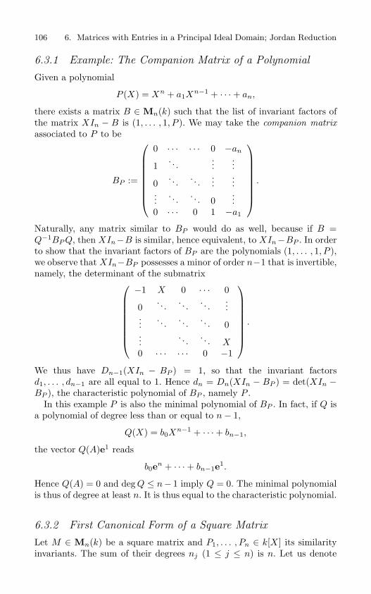
106 6. Matrices with Entries in a Principal Ideal Domain; Jordan Reduction
6.3.1 Example: The Companion Matrix of a Polynomial
Given a polynomial
P (X) = Xn + a1Xn−1 + · · ·+ an,
there exists a matrix B ∈ Mn(k) such that the list of invariant factors ofthe matrix XIn − B is (1, . . . , 1, P ). We may take the companion matrixassociated to P to be
BP :=
0 · · · · · · 0 −an
1. . .
......
0. . .
. . ....
......
. . . . . . 0...
0 · · · 0 1 −a1
.
Naturally, any matrix similar to BP would do as well, because if B =Q−1BP Q, then XIn−B is similar, hence equivalent, to XIn−BP . In orderto show that the invariant factors of BP are the polynomials (1, . . . , 1, P ),we observe that XIn−BP possesses a minor of order n−1 that is invertible,namely, the determinant of the submatrix
−1 X 0 · · · 0
0. . . . . . . . .
......
. . . . . . . . . 0...
. . . . . . X0 · · · · · · 0 −1
.
We thus have Dn−1(XIn − BP ) = 1, so that the invariant factorsd1, . . . , dn−1 are all equal to 1. Hence dn = Dn(XIn − BP ) = det(XIn −BP ), the characteristic polynomial of BP , namely P .
In this example P is also the minimal polynomial of BP . In fact, if Q isa polynomial of degree less than or equal to n− 1,
Q(X) = b0Xn−1 + · · ·+ bn−1,
the vector Q(A)e1 reads
b0en + · · ·+ bn−1e1.
Hence Q(A) = 0 and deg Q ≤ n− 1 imply Q = 0. The minimal polynomialis thus of degree at least n. It is thus equal to the characteristic polynomial.
6.3.2 First Canonical Form of a Square Matrix
Let M ∈ Mn(k) be a square matrix and P1, . . . , Pn ∈ k[X ] its similarityinvariants. The sum of their degrees nj (1 ≤ j ≤ n) is n. Let us denote

6.3. Similarity Invariants and Jordan Reduction 107
by M (j) ∈ Mnj (k) the companion matrix of the polynomial Pj . Let usform the matrix M ′, block-diagonal, whose diagonal blocks are the M (j)’s.The few first polynomials Pj are generally constant (we shall see belowthat the only case where P1 is not constant corresponds to M = αIn), andthe corresponding blocks are empty, as are the corresponding rows andcolumns. To be precise, the actual number m of diagonal blocks is equal tothe nuber of nonconstant similarity invariants.
Since the matrix XInj − M (j) is equivalent to the matrix N (j) =diag(1, . . . , 1, Pj), we have
XInj −M (j) = P (j)N (j)Q(j),
where P (j), Q(j) ∈ GLnj (k[X ]). Let us form matrices P, Q ∈ GLn(k[X ])by
P = diag(P (1), . . . , P (n)), Q = diag(Q(1), . . . , Q(n)).
We obtain
XIn −M ′ = PNQ, N = diag(N (1), . . . , N (n)).
Here N is a diagonal matrix, whose diagonal entries are the similarityinvariants of M , up to the order. In fact, each nonconstant Pj appearsin the associated block N (j). The other diagonal terms are the constant1, which occurs n−m times; these are the polynomials P1, . . . , Pn−m, asexpected. Conjugating by a permutation matrix, we obtain that XIn−M ′
is equivalent to the matrix diag(P1, . . . , Pn). Hence XIn−M ′ is equivalentto XIn −M . From Theorem 6.3.1, M and M ′ are similar.
Theorem 6.3.4 Let k be a field, M ∈ Mn(k) a square matrix, andP1, . . . , Pn its similarity invariants. Then M is similar to the block-diagonal matrix M ′ whose jth diagonal block is the companion matrix ofPj.
The matrix M ′ is called the first canonical form of M , or the Frobeniuscanonical form of M .
Remark: If L is an extension of k (namely, a field containing k) and M ∈Mn(k), then M ∈Mn(L). Let P1, . . . , Pn be the similarity invariants of Mas a matrix with entries in k. Then XIn−M = P diag(P1, . . . , Pn)Q, whereP, Q ∈ GLn(k[X ]). Since P, Q, their inverses, and the diagonal matrix alsobelong to Mn(L[X ]), P1, . . . , Pn are the similarity invariants of M as amatrix with entries in L. In other words, the similarity invariants dependon M but not on the field k. To compute them, it is enough to placeourselves in the smallest possible field, namely that spanned by the entriesof M . The same remark holds true for the first canonical form. As we shallsee in the next section, it is no longer true for the second canonical form,which is therefore less canonical.
We end this paragraph with a characterization of the minimal polyno-mial.

108 6. Matrices with Entries in a Principal Ideal Domain; Jordan Reduction
Theorem 6.3.5 Let k be a field, M ∈ Mn(k) a square matrix, andP1, . . . , Pn its similarity invariants. Then Pn is the minimal polynomialof M . In particular, the minimal polynomial does not depend on the fieldunder consideration, as long as it contains the entries of M .
ProofWe use the first canonical form M ′ of M . Since M ′ and M are similar,
they have the same minimal polynomial. One thus can assume that M isin the canonical form M = diag(M1, . . . , Mn), where Mj is the companionmatrix of Pj . Since Pj(Mj) = 0 (Cayley–Hamilton, theorem 2.5.1) andPj |Pn, we have Pn(Mj) = 0 and thus Pn(M) = 0n. Hence, the minimalpolynomial QM divides Pn. Conversely, Q(M) = 0n implies Q(Mn) = 0.Since Pn is the minimal polynomial of Mn, Pn divides Q. Finally, Pn = QM .
Finally, since the similarity invariants do not depend on the choice of thefield, Pn also does not depend on this choice.
Warning: One may draw an incorrect conclusion if one applies Theorem6.3.5 carelessly. Given a matrix M ∈ Mn(ZZ), one can define a matrixM(p) in Mn(ZZ/pZZ) by reduction modulo p (p a prime number). But theminimal polynomial of M(p) is not necessarily the reduction modulo p ofQM . Here is an example: Let us take n = 2 and
M =(
2 20 2
).
Then QM divides PM = (X − 2)2, but QM = X − 2, since M = 2I2. HenceQM = (X− 2)2. On the other hand, M(2) = 02, whose minimal polynomialis X , which is different from X2, the reduction modulo 2 of QM .
The explanation of this phenomenon is the following. The matrices Mand M(2) are composed of scalars of different natures. There is no fieldL containing simultaneously ZZ and ZZ/2ZZ. There is thus no context inwhich Theorem 6.3.5 could be applied.
6.3.3 Second Canonical Form of a Square Matrix
We now decompose the similarity invariants of M into products of irre-ducible polynomials. This decomposition depends, of course, on the choiceof the field of scalars. Denoting by p1, . . . , pt the list of distinct irreducible(in k[X ]) factors of Pn, we have
Pj =t∏
k=1
pα(j,k)k , 1 ≤ j ≤ n
(because Pj divides Pn), where the α(j, k) are nondecreasing with respectto j, since Pj divides Pj+1.

6.3. Similarity Invariants and Jordan Reduction 109
Definition 6.3.2 The elementary divisors of the matrix M ∈ Mn(k) arethe polynomials p
α(j,k)k for which the exponent α(j, k) is nonzero. The mul-
tiplicity of an elementary divisor pmk is the number of solutions j of the
equation α(j, k) = m. The list of elementary divisors is the sequence ofthese polynomials, repeated with their multiplicities.
Let us begin with the case of the companion matrix N of some polynomialP . Its similarity invariants are (1, . . . , 1, P ) (see above). Let Q1, . . . , Qt beits elementary divisors (we observe that each has multiplicity one). We thenhave P = Q1 · · ·Qt, while the Ql’s are pairwise coprime. To each Ql weassociate its companion matrix Nl, and we form a block-diagonal matrixN ′ := diag(N1, . . . , Nt). Since each Nl − XIl is equivalent to a diagonalmatrix
1
. . .1
Ql
in Mn(l)(k[X ]), the whole matrix N ′ −XIn is equivalent to
Q :=
1. . . O
1Q1
O. . .
Qt
.
Let us now compute the similarity invariants of N ′, that is, the invariantfactors of Q. It will be enough to compute the greatest common divisorDn−1 of the minors of size n− 1. Taking into account the principal minorsof Q, we see that Dn−1 must divide every product of the form∏
l=k
Ql, 1 ≤ k ≤ t.
Since the Ql’s are pairwise coprime, this implies that Dn−1 = 1. Thismeans that the list of similarity invariants of N ′ has the form (1, . . . , 1, ·),where the last polynomial must be the characteristic polynomial of N ′.This polynomial is the product of the characteristic polynomials of theNl’s. These being equal to the Ql’s, the characteristic polynomial of N ′ isP . Finally, N and N ′ have the same similarity invariants and are thereforesimilar.
Now let M be a general matrix in Mn(k). We apply the former reductionto every diagonal block Mj of its Frobenius canonical form. Each Mj issimilar to a block-diagonal matrix whose diagonal blocks are companionmatrices corresponding to the elementary divisors of M entering into the

110 6. Matrices with Entries in a Principal Ideal Domain; Jordan Reduction
factorization of the jth invariant polynomial of M . We have thus provedthe following statement.
Theorem 6.3.6 Let Q1, . . . , Qs be the elementary divisors of M ∈Mn(k). Then M is similar to a block-diagonal matrix M ′ whose diagonalblocks are companion matrices of the Ql’s.
The matrix M ′ is called the second canonical form of M .
Remark: The exact computation of the second canonical form of a givenmatrix is impossible in general, in contrast to the case of the first form.Indeed, if there were an algorithmic construction, it would provide an algo-rithm for factorizing polynomials into irreducible factors via the formationof the companion matrix, a task known to be impossible if k = IR or CC.Recall that one of the most important results in Galois theory, known asAbel’s theorem, states the impossibility of solving a general polynomialequation of degree at least five with complex coefficients, using only thebasic operations and the extraction of roots of any order.
6.3.4 Jordan Form of a Matrix
When the characteristic polynomial splits over k, which holds, for instance,if the field k is algebraically closed, the elementary divisors have the form(X − a)r for a ∈ k and r ≥ 1. In that case, the second canonical form canbe greatly simplified by replacing the companion matrix of the monomial(X − a)r by its Jordan block
J(a; r) :=
a 1 0 · · · 0
0. . . . . . . . .
......
. . . . . . . . . 0...
. . .. . . 1
0 · · · · · · 0 a
.
In fact, the characteristic polynomial of J(a; r) (of size r × r) is (X − a)r,while the matrix XIr−J(a; r) possesses an invertible minor of order r− 1,namely
−1 0 · · · 0
X − a. . . . . .
.... . . . . . 0
X − a −1
,
which is obtained by deleting the first column and the last row. Again, thisshows that Dn−1(XIr − J) = 1, so that the invariant factors d1, . . . , dr−1
are equal to 1. Hence dr = Dr(XIr − J) = det(XIr − J) = (X − a)r. Its

6.4. Exercises 111
invariant factors are thus 1, . . . , 1, (X − a)r. Hence we have the followingtheorem.
Theorem 6.3.7 When an elementary divisor of M is (X − a)r, one may,in the second canonical form of M , replace its companion matrix by theJordan block J(a; r).
Corollary 6.3.1 If the characteristic polynomial of M splits over k, thenM is similar to a block-diagonal matrix whose jth diagonal block is a Jordanblock J(aj ; rj). This form is unique, up to the order of blocks.
Corollary 6.3.2 If k is algebraically closed (for example if k = CC), thenevery square matrix M is similar to a block-diagonal matrix whose jthdiagonal block is a Jordan block J(aj ; rj). This form is unique, up to theorder of blocks.
6.4 Exercises
See also the exercise 12 in Chapter 7.
1. Show that every principal ideal domain is a unique factorizationdomain.
2. Verify that the characteristic polynomial of the companion matrix ofa polynomial P is equal to P .
3. Let k be a field and M ∈ Mn(k). Show that M , MT have the samerank and that in general, the rank of MT M is less than or equalto that of M . Show that the equality of these ranks always holds ifk = IR, but that strict inequality is possible, for example with k = CC.
4. Compute the elementary divisors of the matrices
22 23 10 −9812 18 16 −38−15 −19 −13 586 7 4 −25
,
0 −21 −56 −9618 36 52 −8−12 −17 −16 383 2 −2 −20
and
44 89 120 −320 −12 −32 −56−14 −20 −16 498 14 16 −16
in Mn(CC). What are their Jordan reductions?
5. (Lagrange’s theorem)

112 6. Matrices with Entries in a Principal Ideal Domain; Jordan Reduction
Let K be a field and A ∈ Mn(K). Let X, Y ∈ Kn be vectors suchthat XT AY = 0. We normalize by XT AY = 1 and define
B := A− (AY )(XT A).
Show that in the factorization
PAQ =(
Ir 00 0n−r
), P, Q ∈ GLn(K),
one can choose Y as the first column of Q and XT as the first row ofP . Deduce that rkB = rkA− 1.More generally, show that if X, Y ∈Mn×m(K), XT AY ∈ GLm(K),and if
B := A− (AY )(XT AY )−1(XT A),
then rk B = rk A−m.If A ∈ Symn(IR) and if A is positive semidefinite, and if X = Y ,show that B is also positive semidefinite.
6. For A ∈Mn(CC), consider the linear differential equation in CCn
dx
dt= Ax. (6.1)
(a) Let P ∈ GLn(CC) and let t → x(t) be a solution of (6.1). Whatis the differential equation satisfied by t → Px(t)?
(b) Let (X−a)m be an elementary divisor of A. Show that for everyk = 0, . . . , m− 1, (6.1) possesses solutions of the form eatQk(t),where Qk is a complex-valued polynomial map of degree k.
7. Consider the following differential equation of order n in CC:
x(n)(t) + a1x(n−1)(t) + · · ·+ anx(t) = 0. (6.2)
(a) Define P (X) = Xn + a1Xn−1 + · · · + an and let M be the
companion matrix of P . Let
P (X) =∏a∈A
(X − a)na
be the factorization of P into irreducible factors. Compute theJordan form of M .
(b) Using either the previous exercise or arguing directly, show thatthe set of solutions of (6.2) is spanned by the solutions of theform
t → eatR(t), R ∈ CC[X ], deg R < na.
8. Consider a linear recursion of order n in a field K
um+n + a1um+n−1 + · · ·+ anum = 0, m ∈ IN. (6.3)

6.4. Exercises 113
With the notation of the previous exercise, show that the set ofsolutions of (6.3) is spanned by the solutions of the form
(amR(m))m∈IN , R ∈ CC[X ], deg R < na.
9. Let n ≥ 2 and let M ∈ Mn(ZZ) be the matrix defined by mij =i + j − 1:
M =
1 2 · · · n
2 . . . . . ....
... . . . . . ....
n · · · · · · 2n− 1
.
(a) Show that M has rank 2 (you may look for two vectors x, y ∈ ZZn
such that mij = xixj − yiyj).(b) Compute the invariant factors of M in Mn(ZZ) (the equivalent
diagonal form is obtained after five elementary operations).
10. The ground field is CC.
(a) Define
N = J(0; n), B =
. . . 0 1... . . . . . . 0
0 . . . . . ....
1 0 . . .
.
Compute NB, BN , and BNB. Show that S := 1√2(I + iB) is
unitary.(b) Deduce that N is similar to
12
0 1 0 . . . 0
1. . . . . . . . .
...
0. . . . . . . . . 0
.... . . . . . . . . 1
0 . . . 0 1 0
+i
2
0 . . . 0 −1 0... . . . . . . . . . 10 . .
.. .
.. .
.0
−1 . . . . . . . . ....
0 1 0 . . . 0
.
(c) Deduce that every matrix M ∈ Mn(CC) is similar to a complexsymmetric matrix. Compare with the real case.

7Exponential of a Matrix, PolarDecomposition, and Classical Groups
7.1 The Polar Decomposition
The polar decomposition of matrices is defined by analogy with that in thecomplex plane: If z ∈ CC∗, there exists a unique pair (r, q) ∈ (0, +∞)× S1
(S1 denotes the unit circle, the set of complex numbers of modulus 1) suchthat z = rq. If z acts on CC (or on CC∗) by multiplication, this action canbe decomposed as the product of a rotation of angle θ (where q = exp(iθ))with a homothety of ratio r > 0. The fact that these two actions commuteis a consequence of the commutativity of the multiplicative group CC∗; thisproperty does not hold for the polar decomposition in GLn(k), k = IR orCC, because the general linear group is not commutative.
Let us recall that HPDn denotes the (open) cone of matrices of Mn(CC)that are Hermitian positive definite, while Un denotes the group of unitarymatrices. In Mn(IR), SPDn is the set of symmetric positive definite ma-trices, and On is the orthogonal group. The group Un is compact, since itis closed and bounded in Mn(CC). Indeed, the columns of unitary matricesare unit vectors, so that Un is bounded. On the other hand, Un is definedby an equation U∗U = In, where the map U → U∗U is continuous; henceUn is closed. By the same arguments, On is compact.
Polar decomposition is a fundamental tool in the theory of finite-dimensional Lie groups and Lie algebras. For this reason, it is intimatelyrelated to the exponential map. We shall not consider these two notionshere in their full generality, but we shall restrict attention to their matricialaspects.

7.1. The Polar Decomposition 115
Theorem 7.1.1 For every M ∈ GLn(CC), there exists a unique pair
(H, Q) ∈ HPDn ×Un
such that M = HQ. If M ∈ GLn(IR), then (H, Q) ∈ SPDn ×On.The map M → (H, Q), called the polar decomposition of M , is a
homeomorphism between GLn(CC) and HPDn ×Un (respectively betweenGLn(IR) and SPDn ×On).
Theorem 7.1.2 Let H be a positive definite Hermitian matrix. There ex-ists a unique positive definite Hermitian matrix h such that h2 = H. If His real-valued, then so is h. The matrix h is called the square root of H,and is denoted by h =
√H.
ProofWe prove Theorem 7.1.1 and obtain Theorem 7.1.2 as a by-product.Existence. Since MM∗ ∈ HPDn, we can diagonalize MM∗ by a
unitary matrix
MM∗ = U∗DU, D = diag(d1, . . . , dn),
where dj ∈ (0, +∞). The matrix H := U∗ diag(√
d1, . . . ,√
dn)U is Hermi-tian positive definite and satisfies H2 = HH∗ = MM∗. Then Q := H−1Msatisfies Q∗Q = M∗H−2M = M∗(MM∗)−1M = In, hence Q ∈ Un. IfM ∈ Mn(IR), then clearly MM∗ is real symmetric. In fact, U is orthogo-nal and H is real symmetric. Hence Q is real orthogonal. Note: H is calledthe square root of MM∗.
Uniqueness. Let M = H ′Q′ be another suitable decomposition. ThenN := H−1H ′ = Q(Q′)−1 is unitary, so that Sp(N) ⊂ S1. Let S ∈ HPDn
be a positive definite Hermitian square root of H ′ (we shall prove belowthat it is unique). Then N is similar to N ′ := SH−1S. However, N ′ ∈HPDn. Hence N is diagonalizable, with real positive eigenvalues. HenceSp(N) = 1, and N is therefore similar, and thus equal, to In.
This proves that the positive definite Hermitian square root of a matrixof HPDn is unique in HPDn, since otherwise, our construction wouldprovide several polar decompositions. We have thus proved Theorem 7.1.2in passing.
Smoothness. The map (H, Q) → HQ is polynomial, hence continuous.Conversely,, it is enough to prove that M → (H, Q) is sequentially con-tinuous, since GLn(CC) is a metric space. Let (Mk)k∈IN be a convergentsequence in GLn(CC) and let M be its limit. Let us denote by Mk = HkQk
and M = HQ their respective polar decompositions. Let R be a clusterpoint of the sequence (Qk)k∈IN , that is, the limit of some subsequence(Qkl
)l∈IN , with kl → +∞. Then Hkl= Mkl
Q∗kl
converges to S := MR∗.The matrix S is Hermitian positive semidefinite (because it is the limitof the Hkl
’s) and invertible (because it is the product of M and R∗). Itis thus positive definite. Hence, SR is a polar decomposition of M . Theuniqueness part ensures that R = Q and S = H . The sequence (Qk)k∈IN ,

116 7. Exponential of a Matrix, Polar Decomposition, and Classical Groups
which is relatively compact and has at most one cluster point (namely Q),converges to Q. Finally, Hk = MkQ∗
k converges to MQ∗ = H .
Remark: There is as well a polar decomposition M = QH with the sameproperties. We shall use one or the other depending on the context. Wewarn the reader, however, that for a given matrix, the two decompositionsdo not coincide. For example, in M = HQ, H is the square root of MM∗,though in M = QH, it is the square root of M∗M .
7.2 Exponential of a Matrix
The ground field is here k = CC. By restriction, we can also treat the casek = IR.
For A in Mn(CC), the series
∞∑k=0
1k!
Ak
converges normally (which means that the series of norms is convergent),since for any matrix norm, we have
∞∑k=0
∥∥∥∥ 1k!
Ak
∥∥∥∥ ≤∞∑
k=0
1k!‖A‖k = exp ‖A‖.
Since Mn(CC) is complete, the series is convergent, and the estimation aboveshows that it converges uniformly on every compact set. Its sum, denotedby expA, thus defines a continuous map exp : Mn(CC) → Mn(CC), calledthe exponential. When A ∈Mn(IR), we have expA ∈Mn(IR).
Given two matrices A and B in general position, the binomial formulais not valid: (A + B)k does not necessarily coincide with
j=k∑j=0
(kj
)AjBk−j .
It thus follows that exp(A + B) differs in general from expA · expB. Acorrect statement is the following.
Proposition 7.2.1 Let A, B ∈ Mn(CC) be commuting matrices; that is,AB = BA. Then exp(A + B) = (expA)(expB).
ProofThe proof proceeds in exactly the same way as for the exponential of
complex numbers. We observe that since the series defining the expo-nential of a matrix is normally convergent, we may compute the product

7.2. Exponential of a Matrix 117
(expA)(expB) by multiplying term by term the series
(expA)(exp B) =∞∑
j,k=0
1j!k!
AjBk.
In other words,
(expA)(expB) =∞∑l=0
1l!
Cl,
where
Cl :=∑
j+k=l
l!j!k!
AjBk.
From the assumption AB = BA, we know that the binomial formula holds.Therefore, Cl = (A + B)l, which proves the proposition.
Noting that exp 0n = In and that A and −A commute, we derive thefollowing corollary.
Corollary 7.2.1 For every A ∈ Mn(CC), exp A is invertible, and itsinverse is exp(−A).
Given two conjugate matrices B = P−1AP , we have Bk = P−1AkP foreach integer k and thus
exp(P−1AP ) = P−1(expA)P. (7.1)
If D = diag(d1, . . . , dn) is diagonal, we have
expD = diag(expd1, . . . , exp dn).
Of course, this formula, or more generally (7.1), can be combined withJordan reduction in order to compute the exponential of a given matrix.Let us keep in mind, however, that Jordan reduction cannot be carried outexplicitly.
Let us introduce a real parameter t and let us define a function g byg(t) = exp tA. From Proposition 7.2.1, we see that g satisfies the functionalequation
g(s + t) = g(s)g(t). (7.2)
On the other hand, g(0) = In, and we have
g(t)− g(0)t
−A =∞∑
k=2
tk−1
k!Ak.
Using any matrix norm, we deduce that∥∥∥∥g(t)− g(0)t
−A
∥∥∥∥ ≤ e‖tA‖ − 1− ‖tA‖|t| ,

118 7. Exponential of a Matrix, Polar Decomposition, and Classical Groups
from which we obtain
limt→0
g(t)− g(0)t
= A.
We conclude that g has a derivative at t = 0, with g′(0) = A. Using thefunctional equation (7.2), we then obtain that g is differentiable everywhere,with
g′(t) = lims→0
g(t)g(s)− g(t)s
= g(t)A.
We observe that we also have
g′(t) = lims→0
g(s)g(t)− g(t)s
= Ag(t).
From either of these differential equations we see that g is actually infinitelydifferentiable. We shall retain the formula
d
dtexp tA = A exp tA = (exp tA)A. (7.3)
This differential equation is sometimes the most practical way to computethe exponential of a matrix. This is of particular relevance when A has realentries but has at least one nonreal eigenvalue if one wishes to avoid theuse of complex numbers.
Proposition 7.2.2 For every A ∈Mn(CC),
det expA = exp TrA. (7.4)
ProofWe could deduce (7.4) directly from (7.3). Here is a more elementary
proof. We begin with a reduction of A of the form A = P−1TP , where Tis upper triangular. Since T k is still triangular, with diagonal entries equalto tkjj , exp T is triangular too, with diagonal entries equal to exp tjj . Hence
det expT =∏j
exp tjj = exp∑
j
tjj = expTr T.
This is the expected formula, since expA = P−1(expT )P .
Since (M∗)k = (Mk)∗, we see easily that (exp M)∗ = exp(M∗). Inparticular, the exponential of a skew-Hermitian matrix is unitary, for then
(expM)∗ exp M = exp(M∗) exp M = exp(−M) expM = In.
Similarly, the exponential of a Hermitian matrix is Hermitian positivedefinite, because
exp M =(
exp12M
)∗exp
12M.

7.2. Exponential of a Matrix 119
This calculation also shows that if M is Hermitian, then√
expM = exp12M.
We shall use the following more precise statement:
Proposition 7.2.3 The map exp : Hn → HPDn is a homeomorphism(that is, a bicontinuous bijection).
Proof
Injectivity: Let A, B ∈ Hn with exp A = expB =: H . Then
exp12A =
√H = exp
12B.
By induction, we have
exp 2−mA = exp 2−mB, m ∈ ZZ.
Substracting In, multiplying by 2m, and passing to the limit as m →+∞, we obtain
d
dt
∣∣∣∣t=0
exp tA =d
dt
∣∣∣∣t=0
exp tB;
that is, A = B.
Surjectivity: Let H ∈ HPDn be given. Then H = U∗ diag(d1, . . . , dn)U ,where U is unitary and dj ∈ (0, +∞). From above, we know thatH = expM for
M := U∗ diag(log d1, . . . , log dn)U,
which is Hermitian.
Continuity: The continuity of exp has already been proved. Let us in-vestigate the continuity of the reciprocal map. Let (H l)l∈IN be asequence in HPDn that converges to H ∈ HPDn. We denote byM l, M ∈ Hn, the Hermitian matrices whose exponentials are H l andH . The continuity of the spectral radius gives
liml→+∞
ρ(H l) = ρ(H), liml→+∞
ρ((H l)−1
)= ρ
((H)−1
). (7.5)
Since Sp(M l) = log Sp(M l), we have
ρ(M l) = log maxρ(H l), ρ
((H l)−1
). (7.6)
Keeping in mind that the restriction to Hn of the induced norm ‖ ·‖2coincides with that of the spectral radius ρ, we deduce from (7.5, 7.6)that the sequence (M l)l∈IN is bounded. If N is a cluster point of thesequence, the continuity of the exponential implies expN = H . Butthe injectivity shown above implies N = M . The sequence (M l)l∈IN ,bounded with a unique cluster point, is convergent.

120 7. Exponential of a Matrix, Polar Decomposition, and Classical Groups
7.3 Structure of Classical Groups
Proposition 7.3.1 Let G be a subgroup of GLn(CC). We assume that Gis stable under the map M →M∗ and that for every M ∈ G ∩HPDn, thesquare root
√M is an element of G. Then G is stable under polar decompo-
sition. Furthermore, polar decomposition is a homeomorphism between Gand
(G ∩Un)× (G ∩HPDn).
This proposition applies in particular to subgroups of GLn(IR) that arestable under transposition and under extraction of square roots in SPDn.One has then
Ghomeo∼ (G ∩On)× (G ∩ SPDn).
ProofLet M ∈ G be given and let HQ be its polar decomposition. Since
MM∗ ∈ G, we have H2 ∈ G, that is, H ∈ G, by assumption. Finally, wehave Q = H−1M ∈ G. An application of Theorem 7.1.1 finishes the proof.
We apply this general result to the classical groups U(p, q), O(p, q)(where n = p+q) and Spm (where n = 2m). These are respectively the uni-tary group of the Hermitian form |z1|2+ · · ·+ |zp|2−|zp+1|2−· · ·−|zn|2, theorthogonal group of the quadratic form x2
1 + · · ·+x2p−x2
p+1−· · ·−x2n, and
the symplectic group. They are defined by G = M ∈Mn(k)|M∗JM = J,with k = CC for U(p, q), k = IR otherwise. The matrix J equals(
Ip 0p×q
0q×p −Iq
),
for U(p, q) and O(p, q), and (0m Im
−Im 0m
),
for Spm. In each case, J2 = ±In.
Proposition 7.3.2 Let J be a complex n×n matrix satisfying J2 = ±In.The subgroup G of Mn(CC) defined by the equation M∗JM = J is invariantunder polar decomposition. If M ∈ G, then | detM | = 1.
ProofThe fact that G is a group is immediate. Let M ∈ G. Then detJ =
detM∗ detM detJ ; that is, | detM |2 = 1. Furthermore, M∗JM(JM∗) =J2M∗ = ±M∗ = M∗J2. Simplifying by M∗J on the left, there remainsMJM∗ = J , that is, M∗ ∈ G.

7.3. Structure of Classical Groups 121
Observe that, since G is a group, M ∈ G implies (M∗)kJ = JM−k forevery k ∈ IN . By linearity, it follows that p(M∗)J = Jp(M−1) holds forevery polynomial p ∈ IR[X ].
Let us now assume that M ∈ G ∩ HPDn. We then have M =U∗ diag(d1, . . . , dn)U , where U is unitary and the dj ’s are positive realnumbers. Let A be the set formed by the numbers dj and 1/dj. There ex-ists a polynomial p with real entries such that p(a) =
√a for every a ∈ A.
Then we have p(M) =√
M and p(M−1) =√
M−1
. Since M∗ = M , wehave also p(M)J = Jp(M−1); that is,
√MJ = J
√M
−1. Hence
√M ∈ G.
From Proposition 7.3.1, G is stable under polar decomposition.
The main result of this section is the following:
Theorem 7.3.1 Under the hypotheses of Proposition 7.3.2, the group Gis homeomorphic to (G ∩Un)× IRd, for a suitable integer d.
Of course, if G = O(p, q) or Spm, the subgroup G∩Un can also be writtenas G∩On. We call G∩Un a maximal compact subgroup of G, because onecan prove that it is not a proper subgroup of a compact subgroup of G.Another deep result, which is beyond the scope of this book, is that everymaximal compact subgroup of G is a conjugate of G ∩Un. In the sequel,when speaking about the maximal compact subgroup of G, we shall alwayshave in mind G ∩Un.
ProofThe proof amounts to showing that G∩HPDn is homeomorphic to some
IRd. To do this, we define
G := N ∈Mn(k)| exp tN ∈ G, ∀t ∈ IR.Lemma 7.3.1 The set G defined above satifies
G = N ∈Mn(k)|N∗J + JN = 0n.Proof
If N∗J + JN = 0n, let us set M(t) = exp tN . Then M(0) = In and
d
dtM(t)∗JM(t) = M∗(t)(N∗J + JN)M(t) = 0n,
so that M(t)∗JM(t) ≡ J . We thus have N ∈ G. Conversely,, if M(t) :=exp tN ∈ G for every t, then the derivative at t = 0 of M∗(t)JM(t) = Jgives N∗J + JN = 0n.
Lemma 7.3.2 The map exp : G∩Hn → G∩HPDn is a homeomorphism.
ProofWe must show that exp : G ∩ Hn → G ∩ HPDn is onto. Let M ∈
G ∩ HPDn and let N be the Hermitian matrix such that expN = M .Let p ∈ IR[X ] be a polynomial with real entries such that for every λ ∈

122 7. Exponential of a Matrix, Polar Decomposition, and Classical Groups
SpM ∪ SpM−1, we have p(λ) = log λ. Such a polynomial exists, since thenumbers λ are real and positive.
Let N = U∗DU be a unitary diagonalization of N . Then M = expN =U∗(expD)U and M−1 = exp(−N) = U∗ exp(−D)U . Hence, p(M) = Nand p(M−1) = −N . However, M ∈ G implies MJ = JM−1, and thereforeq(M)J = Jq(M−1) for every q ∈ IR[X ]. With q = p, we obtain NJ = −JN .
These two lemmas complete the proof of the theorem, since G ∩Hn is anIR-vector space. The integer d mentionned in the theorem is its dimension.
We wish to warn the reader that neither G, nor Hn is a CC-vector space.We shall see examples in the next section that show that G ∩Hn can benaturally IR-isomorphic to a CC-vector space, which is a source of confusion.One therefore must be cautious when computing d.
The reader eager to learn more about the theory of classical groups isadvised to have a look at the book of R. Mneimne and F. Testard [28] orthe one by A. W. Knapp [24].
7.4 The Groups U(p, q)
Let us begin with the study of the maximal compact subgroup of U(p, q).If M ∈ U(p, q) ∩Un, let us write M blockwise:
M =(
A BC D
),
where A ∈ Mp(CC), etc. The following equations express that M belongsto Un:
A∗A + C∗C = Ip, B∗B + D∗D = Iq, A∗B + C∗D = 0pq.
Similarly, writing that M ∈ U(p, q),
A∗A− C∗C = Ip, D∗D −B∗B = Iq, A∗B − C∗D = 0pq.
Combining these equations, we obtain first C∗C = 0p and B∗B = 0q. Forevery vector X ∈ CCn, we have ‖CX‖22 = X∗C∗CX = 0; hence CX = 0.Finally, C = 0 and similarly B = 0. There remains A ∈ Up and D ∈ Uq .The maximal compact subgroup of U(p, q) is thus isomorphic (not onlyhomeomorphic) to Up ×Uq.
Furthermore, G ∩Hn is the set of matrices
N =(
A BB∗ D
),
where A ∈ Hp, D ∈ Hq, which satisfy NJ + JN = 0n; that is, A = 0p,D = 0q. Hence G ∩ Hn is isomorphic to Mp×q(CC). One therefore hasd = 2pq.

7.5. The Orthogonal Groups O(p, q) 123
Proposition 7.4.1 The unitary group U(p, q) is homeomorphic to Up ×Uq × IR2pq. In particular, U(p, q) is connected.
There remains to show connectivity. It is a straightforward consequence ofthe following lemma.
Lemma 7.4.1 The unitary group Un is connected.
Since GLn(CC) is homeomorphic to Un×HPDn (via polar decomposition),hence to Un ×Hn (via the exponential), it is equivalent to the followingstatement.
Lemma 7.4.2 The linear group GLn(CC) is connected.
ProofLet M ∈ GLn(CC) be given. Define A := CC \ (1 − λ)−1|λ ∈ Sp(M).
The arcwise-connected set A does not contain the origin, nor the pointz = 1, since 0 ∈ Sp(M). There thus exists a path γ joining 0 to 1 in A:γ ∈ C([0, 1]; A), γ(0) = 0 and γ(1) = 1. Let us define M(t) := γ(t)M +(1−γ(t))In. By construction, M(t) is invertible for every t, and M(0) = In,M(1) = M . The connected component of In is thus all of GLn(CC).
7.5 The Orthogonal Groups O(p, q)
The analysis of the maximal compact subgroup and of G∩Hn for the groupO(p, q) is identical to that in the previous paragraph. On the one hand,O(p, q) ∩ On is isomorphic to Op × Oq. On the other hand, G ∩ Hn isisomorphic to Mp×q(IR), which is of dimension d = pq.
Proposition 7.5.1 Let n ≥ 1. The group O(p, q) is homeomorphic to Op×Oq× IRpq. The number of its connected components is two if p or q is zero,four otherwise.
ProofWe must show that On has two connected components. However, On is
the disjoint union of SOn (matrices of determinant +1) and of O−n (matri-
ces of determinant −1). Since O−n = M ·SOn for any matrix M ∈ O−
n (forexample a hyperplane symmetry), there remains to show that the specialorthogonal group SOn is connected, in fact arcwise connected. We use thefollowing property:

124 7. Exponential of a Matrix, Polar Decomposition, and Classical Groups
Lemma 7.5.1 Given M ∈ On, there exists Q ∈ On such that the matrixQ−1MQ has the form
(·) 0 · · · 0
0. . . . . .
......
. . . . . . 00 · · · 0 (·)
, (7.7)
where the diagonal blocks are of size 1×1 or 2×2 and are orthogonal, thoseof size 2× 2 being rotations matrices:
(cos θ sin θ− sin θ cos θ
). (7.8)
Let us apply Lemma 7.5.1 to M ∈ SOn. The determinant of M , whichis the product of the determinants of the diagonal blocks, equals (−1)m,m being the multiplicity of the eigenvalue −1. Since detM = 1, m is even,and we can gather the diagonal −1’s pairwise in order to form matrices ofthe form (7.8), with θ = π. Finally, there exists Q ∈ On such that
M = QT
R1 0 · · · · · · · · · 0
0. . . . . .
......
. . . Rr. . . 0
.... . . 1
. . ....
.... . . . . . 0
0 · · · · · · · · · 0 1
Q,
where each diagonal block Rj is a matrix of planar rotation:
Rj =(
cos θj sin θj
− sin θj cos θj
).
Let us now define a matrix M(t) as above, in which we replace the anglesθj by tθj . We thus obtain a path in SOn, from M(0) = In to M(1) = M .The connected component of In is thus the whole of SOn.
We now prove Lemma 7.5.1: As an orthogonal matrix, M is normal.From Theorem 3.3.1, it decomposes into a matrix of the form (7.7), the1× 1 diagonal blocks being the real eigenvalues. These eigenvalues are ±1,since Q−1MQ is orthogonal. The diagonal blocks 2×2 are direct similitudematrices. However, they are isometries, since Q−1MQ is orthogonal. Hencethey are rotation matrices.

7.5. The Orthogonal Groups O(p, q) 125
7.5.1 Notable Subgroups of O(p, q)
We assume here that p, q ≥ 1, so that O(p, q) has four connectedcomponents. We first describe them.
Let us recall that if M ∈ O(p, q) reads blockwise
M =(
A BC D
),
where A ∈ Mp(IR), etc. Then AT A = CT C + Ip is larger than Ip as asymmetric matrix, so that det A cannot vanish. Similarly, DT D = BT B+Iq
shows that det D does not vanish. The continuous map M → (detA, detD)thus sends O(p, q) to IR∗ × IR∗ (in fact, to (IR \ (−1, 1))2). Since the signmap from IR∗ to −, + is continuous, we may thus define a continuousfunction
O(p, q) σ→ −, +2 ∼ (ZZ/2ZZ)2 ,
M → (sgndetA, sgn det D).
The diagonal matrices whose diagonal entries are ±1 belong to O(p, q). Itfollows that σ is onto. Since σ is continuous, the preimage Gα of an elementα of −, +2 is the union of some connected components of O(p, q); let n(α)be the number of these components. Then n(α) ≥ 1 (σ being onto), and∑
α n(α) equals 4, the number of connected components of O(p, q). Sincethere are four terms in this sum, we obtain n(α) = 1 for every α. Finally,the connected components of O(p, q) are the Gα’s, where α ∈ −, +2.
The left multiplication by an element M of O(p, q) is continuous, bijec-tive, whose inverse (another multiplication) is continuous. It thus induces apermutation of the set π0 of connected components of O(p, q). Since σ in-duces a bijection between π0 and −, +2, there exists thus a permutationqM of −, +2 such that σ(MM ′) = qM (σ(M ′)). Similarly, the multiplica-tion at right by M ′ is an homeomorphism, allowing to define a permutationpM ′ of−, +2 such that σ(MM ′) = pM ′(σ(M)). The equality
pM ′(σ(M)) = qM (σ(M ′))
shows that pM and qM actually depend only on σ(M). In other words,σ(MM ′) depends only on σ(M) and σ(M ′). A direct evaluation in thespecial case of matrices in O(p, q)∩On(IR) leads to the following conclusion.
Proposition 7.5.2 (p, q ≥ 1) The connected components of G = O(p, q)are the sets Gα := σ−1(α), defined by α1 detA > 0 and α2 detD > 0, whena matrix M is written blockwise as above. The map σ : O(p, q)→ −, +2is a surjective group homomorphism; that is, σ(MM ′) = σ(M)σ(M ′). Inparticular:
1. G−1α = Gα;
2. Gα ·Gα′ = Gαα′ .

126 7. Exponential of a Matrix, Polar Decomposition, and Classical Groups
Remark: σ admits a right inverse, namely
α →Mα := diag(α11, 1, . . . , 1, α21).
The group O(p, q) appears, therefore, as the semidirect product of G++
with (ZZ/2ZZ)2.We deduce immediately from the proposition that O(p, q) possesses five
open and closed normal subgroups, the preimages of the five subgroups of(ZZ/2ZZ)2:
• O(p, q) itself;
• G++, which we also denote by G0 (see Exercise 21), the connectedcomponent of the unit element In,
• G++ ∪Gα, for the three other choices of an element α.
One of these groups, namely G++ ∪G−− is equal to the kernel SO(p, q)of the homomorphism M → detM . In fact, this kernel is open and closed,thus is the union of connected components of O(p, q). However the sign ofdetM for M ∈ Gα is that of α1α2, which can be seen directly from thecase of diagonal matrices Mα.
7.5.2 The Lorentz Group O(1, 3)
If p = 1 and q = 3, the group O(1, 3) is isomorphic to the orthogonalgroup of the Lorentz quadratic form dt2 − dx2
1 − dx22 − dx2
3, which definesthe space-time distance in special relativity.1 Each element M of O(1, 3)corresponds to the transformation(
t,x
)→M
(t,x
),
which we still denote by M , by abuse of notation. This transformationpreserve the light cone of equation t2 − x2
1 − x22 − x2
3 = 0. Since it isa homeomorphism of IR4, it permutes the connected components of thecomplement C of that cone. There are three such components (see Figure7.1):
• the convex set C+ := (t, x) | ‖x‖ < t;• the convex set C− := (t, x) | ‖x‖ < −t;• the “ring” A := (t, x) | |t| < ‖x‖.
Clearly, C+ and C− are homeomorphic. For example, they are so via thetime reversal t → −t. However, they are not homeomorphic to A, becausethe latter is homeomorphic to S2× IR2 (here, S2 denotes the unit sphere),
1We have selected a system of units in which the speed of light equals one.

7.6. The Symplectic Group Spn 127
x1
C−
x2
A
C+
t
Figure 7.1. The Lorentz cone.
which is not contractible, while a convex set is always contractible. SinceM is a homeomorphism, one deduces that necessarily, MA = A, whileMC+ = C±, MC− = C∓.
The transformations that preserve C+, and therefore every connectedcomponent of C, form the orthochronous Lorentz group. Its elements arethose that send the vector e0 := (1, 0, 0, 0)T to C+; that is, those for whichthe first component of Me0 is positive. Since this component is A (here itis nothing but a scalar), this group must be G++ ∪G+−.
7.6 The Symplectic Group Spn
Let us study first of all the maximal compact subgroup Spn ∩O2n. If
M =(
A BC D
),
with blocks of size n× n, then M ∈ Spn means that
AT C = CT A, AT D − CT B = In, BT D = DT B,
while M ∈ O2n yields
AT A + CT C = In, BT B + DT D = In, BT A + DT C = 0n.

128 7. Exponential of a Matrix, Polar Decomposition, and Classical Groups
But since MT ∈ Spn, we also have
ABT = BAT , ADT −BCT = In, CDT = DCT .
Let us combine these equations:
B = B(AT A+CT C) = ABT A+(ADT−In)C = A(BT A+DT C)−C = −C.
Similarly,
D = D(AT A+CT C) = (In+CBT )A+CDT C = A+C(BT A+DT C) = A.
Hence
M =(
A B−B A
).
The remaining conditions are
AT A + BT B = In, AT B = BT A.
This amounts to saying that A + iB is unitary. One immediately checksthat the map M → A + iB is an isomorphism from Spn onto Un.
Finally, if
N =(
A BBT D
)
is symmetric and NJ + JN = 02n, we have, in fact,
N =(
A BB −A
),
where A and B are symmetric. Hence G ∩ Sym2n is homeomorphic toSymn × Symn, that is, to IRn(n+1).
Proposition 7.6.1 The symplectic group Spn is homeomorphic to Un ×IRn(n+1).
Corollary 7.6.1 In particular, every symplectic matrix has determinant+1.
Indeed, Proposition 7.6.1 shows that Spn is connected. Since the de-terminant is continuous, with values in −1, 1, it is constant, equal to+1.
7.7 Singular Value Decomposition
As we shall see in Exercise 8 (see also Exercise 12 in Chapter 4), theeigenvalues of the matrix H in the polar decomposition of a given matrixM are of some importance. They are called the singular values of M . Sincethese are the square roots of the eigenvalues of M∗M , one may even speak

7.7. Singular Value Decomposition 129
of the singular values of an arbitrary matrix, not necessarily invertible.Recalling that (see Exercise 17 in Chapter 2) when M is n×m, M∗M andMM∗ have the same nonzero eigenvalues, counting with multiplicities, onemay even speak of the singular values of a rectangular matrix, up to anambiguity concerning the multiplicity of the eigenvalue 0.
The main result of the section is the following.
Theorem 7.7.1 Let M ∈ Mn×m(CC) be given. Then there exist twounitary matrices U ∈ Un, V ∈ Um and a quasi-diagonal matrix
D =
s1
. . .sr
0. . .
,
with s1, . . . , sr ∈ (0, +∞), such that M = UDV . The numbers s1, . . . , sr
are uniquely defined up to permutation; they are the nonzero singular valuesof M . In particular, r is the rank of M .
If M ∈Mn×m(IR), then one may choose U, V to be real orthogonal.
Remark: The factorization given in the theorem is far from being unique,even for invertible square matrices. In fact, the number of real degrees offreedom in that factorization is n2+m2+min(n, m), which is always greaterthan the dimension 2nm of Mn×m(CC) as an IR-vector space.
ProofSince MM∗ is positive semidefinite, we may write its eigenvalues as
s21, . . . , s2
r, 0, . . . , where the sj ’s, the singular values of M , are positivereal numbers. The spectrum of M∗M has the same form, except for themultiplicity of 0. Indeed, the multiplicities of 0 as an eigenvalue of MM∗
and MM∗, respectively, differ by n −m, while the multiplicities of othereigenvalues are the same for both matrices. We set S = diag(s1, . . . , sr).
Since M and MM∗ have the same rank, and since R(MM∗) ⊂ R(M), wehave R(MM∗) = R(M). Since MM∗ is Hermitian, its kernel is R(M)⊥,where orthogonality is relative to the canonical scalar product; with theduality formula, we conclude that kerMM∗ = kerM∗. Now we are inposition to state that
CCn = R(MM∗)⊕⊥ kerM∗.
Therefore, there exists an orthonormal basis u1, . . . ,un of CCn consist-ing of eigenvectors of MM∗, associated to the s2
j ’s, followed by vectors ofkerM∗. Let us form the unitary matrix
U = (u1, . . . ,un).
Written blockwise, we have U = (UR, UK), where
MM∗UR = URS2, M∗UK = 0.

130 7. Exponential of a Matrix, Polar Decomposition, and Classical Groups
Let now define VR := M∗URS−1. From above, we have
V ∗RVR = S−1U∗
RMM∗URS−1 = Ir.
This means that the columns v1, . . . ,vr of VR constitute an orthonormalfamily.
Noting that these column vectors belong to R(M∗), that is, to (kerM)⊥,a subspace of codimension r, we see that v1, . . . ,vr can be extended toan orthonormal basis v1, . . . ,vm of CCm, where vr+1, . . . belong to kerM .Let V =: (VR, VK) be the unitary matrix whose columns are v1, . . .
We now compute blockwise the product U∗MV . From MVK = 0 andM∗U∗
K = 0, we get
U∗MV =(
U∗RMVR 0
0 0
).
Finally, we obtain
U∗RMVR = U∗
RMM∗URS−1 = U∗RURS = S.
7.8 Exercises
1. Show that the square root map from HPDn into itself is continuous.
2. Let M ∈ Mn(k) be given, with k = IR or CC. Show that there ex-ists a polynomial P ∈ k(X), of degree at most n − 1, such thatP (M) = expM . However, show that this polynomial cannot bechosen independently of the matrix.Compute this polynomial when M is nilpotent.
3. For t ∈ IR, define Pascal’s matrix P (t) by pij(t) = 0 if i < j (thematrix is lower triangular) and
pij(t) = ti−j
(i− 1j − 1
)
otherwise. Let us emphasize that for just this once in this book, Pis an infinite matrix, meaning that its indices range over the infiniteset IN∗. Compute P ′(t) and deduce that there exists a matrix L suchthat P (t) = exp(tL). Compute L explicitly.
4. Let I be an interval of IR and t → P (t) be a map of class C1 withvalues in Mn(IR) such that for each t, P (t) is a projector: P (t)2 =P (t).
(a) Show that the rank of P (t) is constant.(b) Show that P (t)P ′(t)P (t) = 0n.

7.8. Exercises 131
(c) Let us define Q(t) := [P ′(t), P (t)]. Show that P ′(t) =[Q(t), P (t)].
(d) Let t0 ∈ I be given. Show that the differential equation U ′ = QUpossesses a unique solution in I such that U(t0) = In. Show thatP (t) = U(t)P (t0)U(t)−1.
5. Show that the set of projectors of given rank p is a connected subsetin Mn(CC).
6. (a) Let A ∈ HPDn and B ∈ Hn be given. Show that AB is di-agonalizable with real eigenvalues (though it is not necessarilyHermitian). Show also that the sum of the multiplicities of thepositive eigenvalues (respectively zero, respectively negative) isthe same for AB as for B.
(b) Let A, B, C be three Hermitian matrices such that ABC ∈ Hn.Show that if three of the matrices A, B, C, ABC are positivedefinite, then the fourth is positive definite too.
7. Let M ∈ GLn(CC) be given and M = HQ be its polar decomposition.Show that M is normal if and only if HQ = QH.
8. The deformation of an elastic body is represented at each point by asquare matrix F ∈ GL+
3 (IR) (the sign + expresses that det F > 0).More generally, F ∈ GL+
n (IR) in other space dimensions. The densityof elastic energy is given by a function F →W (F ) ∈ IR+.
(a) The principle of frame indifference says that W (QF ) = W (F )for every F ∈ GL+
n (IR) and every rotation Q. Show that thereexists a map w : SPDn → IR+ such that W (F ) = w(H), whereF = QH is the polar decomposition.
(b) When the body is isotropic, we also have W (FQ) = W (F ), forevery F ∈ GL+
n (IR) and every rotation Q. Show that there existsa map φ : IRn → IR+ such that W (F ) = φ(h1, . . . , hn), wherethe hj are the entries of the characteristic polynomial of H . Inother words, W (F ) depends only on the singular values of F .
9. We use Schur’s norm ‖A‖ = (Tr A∗A)1/2.
(a) If A ∈ Mn(CC), show that there exists Q ∈ Un such that ‖A−Q‖ ≤ ‖A − U‖ for every U ∈ Un. We shall define S := Q−1A.We therefore have ‖S − In‖ ≤ ‖S − U‖ for every U ∈ Un.
(b) Let H ∈ Hn be a Hermitian matrix. Show that exp(itH) ∈ Un
for every t ∈ IR. Compute the derivative at t = 0 of
t → ‖S − exp(itH)‖2
and deduce that S ∈ Hn.(c) Let D be a diagonal matrix, unitarily similar to S. Show that
‖D−In‖ ≤ ‖DU−In‖ for every U ∈ Un. By selecting a suitableU , deduce that S ≥ 0n.

132 7. Exponential of a Matrix, Polar Decomposition, and Classical Groups
(d) If A ∈ GLn(CC), show that QS is the polar decomposition of A.(e) Deduce that if H ∈ HPDn and if U ∈ Un, U = In, then
‖H − In‖ < ‖H − U‖.(f) Finally, show that if H ∈ Hn, H ≥ 0n and U ∈ Un, then
‖H − In‖ ≤ ‖H − U‖.10. Let A ∈Mn(CC) and h ∈ CC. Show that In − hA is invertible as soon
as |h| < 1/ρ(A). One then denotes its inverse by R(h; A).
(a) Let r ∈ (0, 1/ρ(A)). Show that there exists a c0 > 0 such thatfor every h ∈ CC with |h| ≤ r, we have
‖R(h; A)− ehA‖ ≤ c0|h|2.(b) Verify the formula
Cm −Bm = (C −B)Cm−1 + · · ·+ Bl−1(C −B)Cm−l + · · ·+ · · ·+ Bm−1(C −B),
and deduce the bound
‖R(h; A)m − emhA‖ ≤ c0m|h|2ec2m|h|,
when |h| ≤ r and m ∈ IN .(c) Show that for every t ∈ CC,
limm→+∞R(t/m; A)m = etA.
11. (a) Let J(a; r) be a Jordan block of size r, with a ∈ CC∗. Let b ∈ CC besuch that a = eb. Show that there exists a nilpotent N ∈Mr(CC)such that J(a; r) = exp(bIr + N).
(b) Show that exp : Mn(CC) → GLn(CC) is onto, but that it is notone-to-one. Deduce that X → X2 is onto GLn(CC). Verify thatit is not onto Mn(CC).
12. (a) Show that the matrix
J2 =( −1 1
0 −1
)
is not the square of any matrix of M2(IR).(b) Show, however, that the matrix J4 := diag(J2, J2) is the square
of a matrix of M4(IR).Show also that the matrix
J3 =(
J2 I2
02 J2
)
is not the square of a matrix of M4(IR).(c) Show that J2 is not the exponential of any matrix of M2(IR).
Compare with the previous exercise.

7.8. Exercises 133
(d) Show that J4 is the exponential of a matrix of M4(IR), but thatJ3 is not.
13. Let An(CC) be the set of skew-Hermitian matrices of size n. Showthat exp : An(CC)→ Un is onto. Hint: If U is unitary, diagonalize it.
14. (a) Let θ ∈ IR be given. Compute expB, where
B =(
0 θ−θ 0
).
(b) Let An(IR) be the set of real skew-symmetric matrices of size n.Show that exp : An(IR)→ SOn is onto. Hint: Use the reductionof direct orthogonal matrices.
15. Let φ : Mn(IR) → IR be a nonnull map satisfying φ(AB) = φ(A)φ(B)for every A, B ∈ Mn(IR). If α ∈ IR, we set δ(α) = |φ(αIn)|1/n. Wehave seen, in Exercise 16 of Chapter 3, that |φ(M)| = δ(det M) forevery M ∈Mn(IR).
(a) Show that on the range of M →M2 and on that of M → exp M ,φ ≡ δ det.
(b) Deduce that φ ≡ δdet on SOn (use Exercise 14) and on SPDn.(c) Show that either φ ≡ δ det or φ ≡ (sgn(det))δ det.
16. Let A be a K-Banach algebra (K = IR or CC) with a unit denoted bye. If x ∈ A, define x0 := e.
(a) Given x ∈ A, show that the series
∑m∈IN
1m!
xm
converges normally, hence converges in A. Its sum is denoted byexp x.
(b) If x, y ∈ A, [x, y] = xy− yx is called the “commutator” of x andy. Show that [x, y] = 0 implies
exp(x + y) = (expx)(exp y), [x, exp y] = 0.
(c) Show that the map t → exp tx is differentiable on IR, with
d
dtexp tx = x exp tx = (exp tx)x.
(d) Let x, y ∈ A be given. Assume that [x, y] commutes with x andy.
i. Show that (exp−tx)xy(exp tx) = xy + t[y, x]x.
ii. Deduce that [exp−tx, y] = t[y, x] exp−tx.

134 7. Exponential of a Matrix, Polar Decomposition, and Classical Groups
iii. Compute the derivative of t → (exp−ty)(exp−tx) exp t(x+y). Finally, prove the Campbell–Hausdorff formula
exp(x + y) = (expx)(exp y)(
exp12[y, x]
).
(e) In A = M3(IR), construct an example that satisfies the abovehypothesis ([x, y] commutes with x and y), where [x, y] isnonzero.
17. Show that the map
H → f(H) := (iIn + H)(iIn −H)−1
induces a homeomorphism from Hn onto the set of matrices of Un
whose spectrum does not contain −1. Find an equivalent of f(tH)−exp(−2itH) as t→ 0.
18. Let G be a group satisfying the hypotheses of Proposition 7.3.2.
(a) Show that G is a Lie algebra, meaning that it is stable under thebilinear map (A, B) → [A, B] := AB −BA.
(b) Show that for t→ 0+,
exp(tA) exp(tB) exp(−tA) exp(−tB) = In + t2[A, B] +O(t3).
Deduce another proof of the stability of G by [·, ·].(c) Show that the map M → [A, M ] is a derivation, meaning that
the Jacobi identity
[A, [B, C]] = [[A, B], C] + [B, [A, C]]
holds.
19. In the case p = 1, q ≥ 1, show that G++ ∪G+− is the set of matricesM ∈ O(p, q) such that the image under M of the “time” vector(1, 0, . . . , 0)T belongs to the convex cone whose equation is
x1 >√
x22 + · · ·+ x2
n.
20. Assume that p, q ≥ 1 and consider the group O(p, q). Define G0 :=G++. Since −In ∈ O(p, q), we denote by (µ, β) the indices for which−In ∈ Gµ,β .If H ∈ GLn(IR), denote by σH the conjugation M → H−1MH .
(a) Let H ∈ G be given. Show that σH (or rather its restriction toG0) is an automorphism of G0.
(b) Let H ∈ Mn(IR) be such that HM = MH for every M ∈ G0.Show that HN = NH for every N ∈ G. Deduce that H is ahomothety.
(c) Let H ∈ G. Show that there exists K ∈ G0 such that σH = σK
if and only if H ∈ G0 ∪Gµ,β .

7.8. Exercises 135
21. A topological group is a group G endowed with a topology for whichthe maps (g, h) → gh and g → g−1 are continuous. Show that in atopological group, the connected component of the unit element isa normal subgroup. Show also that the open subgroups are closed.Give an example of a closed subgroup that is not open.
22. One identifies IR2n with CCn by the map(xy
)→ x + iy.
Therefore, every matrix M ∈ M2n(IR) defines an IR-linear map Mform CCn into itself.
(a) Let
M =(
A BC D
)∈M2n(IR)
be given. Under what condition on the blocks A, B, C, D is themap M CC-linear?
(b) Show that M → M is an isomorphism from Spn∩O2n onto Un.
8Matrix Factorizations
The direct solution (by Cramer’s method) of a linear system Mx = b,where M ∈ GLn(k) (b ∈ kn) is computationally expensive, especially ifone wishes to solve the system many times with various values of b. In thenext chapter we shall study iterative methods for the case k = IR or CC.Here we concentrate on a simple idea: To decompose M as a product PQin such a way that the resolution of the intermediate systems Py = b andQx = y is “cheap.” In general, at least one of the matrices is triangular.For example, if P is lower triangular (pij = 0 if i < j), then its diagonalentries pii are nonzero, and one may solve the system Py = b step by step:
y1 =b1
p11,
...
yi =bi − pi1y1 − · · · − pi,i−1yi−1
pii,
...
yn =bn − pn1y1 − · · · − pn,n−1yn−1
pnn.
The computation of yi needs 2i−1 operations and the final result is obtainedin n2 operations. This is not expensive if one notes that computing theproduct x = M−1b (assuming that M−1 is computed once and for all, anexpensive task) needs 2n2 − n operations.

8.1. The LU Factorization 137
Another example of easily invertible matrices is the orthogonal matrices:If Q ∈ On (or Q ∈ Un), then Qx = y amounts to x = QT y (or x = Q∗y),which is computed in O(n2) operations.
The techniques described below are often called direct solving methods.
8.1 The LU Factorization
Definition 8.1.1 Let M ∈ GLn(k), where k is a field. We say that Madmits an LU factorization if there exist in GLn(k) two matrices L (lowertriangular with 1’s on the diagonal) and U (upper triangular) such thatM = LU .
Remarks:
• The diagonal entries of U are not equal to 1 in general. The LUfactorization is thus asymmetric with respect to L and U .
• The letters L and U recall the shape of the matrices: L for lower andU for upper.
• If there exists an LU factorization (which is unique, as we shall seebelow), then it can be computed by induction on the size of thematrix. The algorithm is provided in the proof of the next theorem.Indeed, if N (p) denotes the matrix extracted from N by keeping onlythe first p rows and columns, we have easily
M (p) = L(p)U (p),
where the matrices L(p) and U (p) have the required properties.
Definition 8.1.2 The leading principal minors of M are the determinantsof the matrices M (p), for 1 ≤ p ≤ n.
Theorem 8.1.1 The matrix M ∈ GLn(k) admits an LU factorization ifand only if its leading principal minors are nonzero. When this conditionis fulfilled, the LU factorization is unique.
ProofLet us begin with uniqueness: If LU = L′U ′, then (L′)−1L = U ′U−1,
which reads L′′ = U ′′, where L′′ and U ′′ are triangular of opposite types,the diagonal entries of L′′ being 1’s. We deduce L′′ = U ′′ = In; that is,L′ = L, U ′ = U .
We next assume that M admits an LU factorization. Then detM (p) =detL(p) detU (p) =
∏1≤j≤p ujj , which is nonzero because U is invertible.
We prove the converse (the existence of an LU factorization) by inductionon the size of the matrices. It is clear if n = 1. Otherwise, let us assumethat the statement is true up to the order n − 1 and let M ∈ GLn(k) be

138 8. Matrix Factorizations
given, with nonzero leading principal minors. We look for L and U in theblockwise form
L =(
L′ 0XT 1
), U =
(U ′ Y0 u
),
with L′, U ′ ∈Mn−1(k), etc. We likewise obtain the description
M =(
M ′ RST m
).
Multiplying blockwise, we obtain the equations
L′U ′ = M ′, L′Y = R, (U ′)T X = S, u = m−XT Y.
By assumption, the leading principal minors of M ′ are nonzero. The induc-tion hypothesis guarantees the existence of the factorization M ′ = L′U ′.Then Y and X are the unique solutions of (triangular) Cramer systems.Finally, u is explicitly given.
Let us now compute the number of operations needed in the computationof L and U . We pass from a factorization in GLn−1(k) to a factorization inGLn(k) by means of the computations of X ((n− 1)(n− 2) operations), Y((n−1)2 operations) and u (2(n−1) operations), for a total of (n−1)(2n−1)operations. Finally, the computation ex nihilo of an LU factorization costsP (n) operations, where P is a polynomial of degree three, with P (X) =2X3/3 + · · · .Proposition 8.1.1 The LU factorization is computable in 2
3n3 + O(n2)operations.
One says that the complexity of the LU factorization is 23n3.
Remark: When all leading principal minors but the last (detM) arenonzero, the proof above furnishes a factorization M = LU , in which U isnot invertible; that is, unn = 0.
8.1.1 Block Factorization
One can likewise perform a blockwise LU factorization. If n = p1 + · · ·+ pr
with pj ≥ 1, the matrices L and U will be block-triangular. The diagonalblocks are square, of respective sizes p1, . . . , pr. Those of L are of the formIpj , while those of U are invertible. A necessary and sufficient conditionfor such a factorization to exist is that the leading principal minors of M ,of orders p1 + · · · + pj (j ≤ r), be nonzero. As above, it is not necessarythat the last minor detM be nonzero. Such a factorization is useful for theresolution of the linear system MX = b if the diagonal blocks of U areeasily inverted, for instance if their sizes are small enough (say pj ≈ √n).
An interesting application of block factorization is the computation ofthe determinant by the Schur complement formula:

8.1. The LU Factorization 139
Proposition 8.1.2 Let M ∈Mn(k) read blockwise
M =(
A BC D
),
where the diagonal blocks are square and A is invertible. Then
detM = detAdet(D − CA−1B).
Of course, this formula generalizes detM = ad− bc, which is valid only for2× 2 matrices. The matrix D−CA−1B is called the Schur complement ofA in M .
ProofSince A is invertible, M admits a blockwise LU factorization, with the
same subdivision. We easily compute
L =(
I 0CA−1 I
), U =
(A B0 D − CA−1B
).
Then detM = detL detU furnishes the expected formula.
Corollary 8.1.1 Let M ∈ GLn(k), with n = 2m, read blockwise
M =(
A BC D
), A, B, C, D ∈ GLm(k).
Then
M−1 =(
(A−BD−1C)−1 (C −DB−1A)−1
(B −AC−1D)−1 (D − CA−1B)−1
).
ProofWe can verify the formula by multiplying by M . The only point to show is
that the inverses are meaningful, that is, that A−BD−1C, . . . are invertible.Because of the symmetry of the formulas, it is enough to check it for a singleterm, namely D − CA−1B. However, det(D − CA−1B) = detM/ detA,which is nonzero by assumption.
We might add that as soon as M ∈ GLn(k) and A ∈ GLp(k) (even ifp = n/2), then
M−1 =( · ·· (D − CA−1B)−1
),
because M admits the blockwise LU factorization and
M−1 = U−1L−1 =(
A−1 ·0 (D − CA−1B)−1
)·(
I 0· I
).

140 8. Matrix Factorizations
8.1.2 Complexity of Matrix Inversion
We can now show that the complexity of inverting a matrix is not higherthan that of matrix multiplication, at equivalent sizes. We assume here thatk = IR or CC.
Notation 8.1.1 We denote by Jn the number of operations in k used inthe inversion of an n× n matrix, and by Pn the number of operations (ink) used in the product of two n× n matrices.
Of course, the number Jn must be understood for generic matrices, thatis, for matrices within a dense open subset of Mn(k). More important,Jn, Pn also depend on the algorithm chosen for inversion or for multipli-cation. In the sequel we wish to adapt the inversion algorithm to the oneused for multiplication.
Let us examine first of all the matrices whose size n has the form 2k.We decompose the matrices M ∈ GLn(k) blockwise, with blocks of size
n/2 × n/2. The condition A ∈ GLn/2(k) defines a dense open set, sinceM → det A is a nonzero polynomial. Suppose that we are given an inver-sion algorithm for generic matrices in GLn/2(k) in jk−1 operations. Thenblockwise LU factorization and the formula M−1 = U−1L−1 furnish aninversion algorithm for generic matrices in GLn(k). We can then boundjk by means of jk−1 and the number πk−1 = P2k−1 of operations used inthe computation of the product of two matrices of size 2k−1 × 2k−1. Weshall denote also by σk = 22k the number of operations involved in thecomputation of the sum of matrices in M2k(k).
To compute M−1, we first compute A−1, then CA−1, which gives usL−1 in jk−1 + πk−1 operations. Then we compute (D − CA−1B)−1 (thisamounts to σk−1 + πk−1 + jk−1 operations) and A−1B(D − CA−1B)−1
(cost: 2πk−1), which furnishes U−1. The computation of U−1L−1 is doneat the cost σk−1 + 2πk−1. Finally,
jk ≤ 2jk−1 + 2σk−1 + 6πk−1.
In other words,
2−kjk − 21−kjk−1 ≤ 2k−1 + 3 · 21−kπk−1. (8.1)
The complexity of the product in Mn(k) obeys the inequalities
n2 ≤ Pn ≤ n2(2n− 1).
The first inequality is due to the number of data (2n2) and the fact thateach operation involves only two of them. The second is given by the naivealgorithm that consists in computing n2 scalar products.
Lemma 8.1.1 If Pn ≤ cαnα (with 2 ≤ α ≤ 3), then jl ≤ Cαπl, whereCα = 1 + 3cα/(2α−1 − 1).
It is enough to sum (8.1) from k = 1 to l and use the inequality 1 + q +· · ·+ ql−1 ≤ ql/(q − 1) for q > 1.

8.1. The LU Factorization 141
When n is not a power of 2, we obtain M−1 by computing the inverse of ablock-diagonal matrix diag(M, I), whose size N satisfies n ≤ N = 2l < 2n.We obtain Jn ≤ jl ≤ Cαπl. Finally, we have the following result.
Proposition 8.1.3 If the complexity Pn of the product in Mn(CC) isbounded by cαnα, then the complexity Jn of inversion in GLn(CC) isbounded by dαnα, where
dα =(
1 +3cα
2α−1 − 1
)2α.
That can be summarized as follows:
Those who know how to multiply know also how to invert.
8.1.3 Complexity of the Matrix Product
The ideas that follow apply to the product of rectangular matrices, but forthe sake of simplicity, we present only the case of square matrices.
As we have seen above, the complexity Pn of matrix multiplication inMn(k) is O(n3). However, better algorithms will allow us to improve theexponent 3. The simplest and oldest one is Strassen’s algorithm, whichuses a recursion. We note first that there exists a way of computing theproduct of two 2× 2 matrices by means of 7 multiplications and 18 addi-tions. Two features of Strassen’s formula are essential. First, the number ofmultiplications that it involves is stricly less than that (eight) of the naivealgorithm. The second is that the method is valid when the matrices haveentries in a noncommutative ring, and so it can be employed for two matri-ces M, N ∈Mn(k), considered as elements of M2(A), with A := Mn/2(k).This trick yields
Pn ≤ 7Pn/2 + 9n2/2.
For n = 2l, we then have
7−lπl − 71−lπl−1 ≤ 92
(47
)l
,
which, after summation from k = 1 to l, gives
7−lπl ≤ 92
11− 4/7
,
because of 47 < 1. Finally,
πl ≤ 212
7l.
When n is not a power of two, one chooses l such that n ≤ 2l < 2n and weobtain the following result.

142 8. Matrix Factorizations
Proposition 8.1.4 The complexity of the multiplication of n×n matricesis O(nα), with α = log 7/ log 2 = 2.807 . . . More precisely,
Pn ≤ 1472
nlog 7log 2 .
The exponent α can be improved, at the cost of greater complication and alarger constant cα. The best exponent known in 1997, due to Coppersmithand Winograd [11], is α = 2.376 . . . A rather complete analysis can befound in the book by P. Burgisser, M. Clausen, and M. A. Shokrollahi [7].
Here is Strassen’s formula [33]. Let M, N ∈M2(A), with
M =(
a bc d
), N =
(x yz t
).
One first forms the expressions x1 = (a + d)(x + t), x2 = (c + d)x, x3 =a(y−t), x4 = d(z−x), x5 = (a+b)t, x6 = (c−a)(x+y), x7 = (b−d)(z+t).Then one computes the product
MN =(
x1 + x4 − x5 + x7 x3 + x5
x2 + x4 x1 − x2 + x3 + x6
).
8.2 Choleski Factorization
In this section k = IR, and we consider symmetric positive definite matrices.
Theorem 8.2.1 Let M ∈ SPDn. Then there exists a unique lower trian-gular matrix L ∈Mn(IR), with strictly positive diagonal entries, satisfyingM = LLT .
ProofLet us begin with uniqueness. If L1 and L2 have the properties stated
above, then In = LLT , for L = L−12 L1, which still has the same form. In
other words, L = L−T , where both sides are triangular matrices, but ofopposite types (lower and upper). The equality shows that L is actuallydiagonal, with L2 = In. Since its diagonal is positive, we obtain L = In;that is, L2 = L1.
We shall give two constructions of L.
First method. The matrix M (p) is positive definite (test the quadraticform induced by M on the linear subspace IRp × 0). The lead-ing principal minors of M are thus nonzero and there exists an LUfactorization M = L0U0. Let D be the diagonal of U0, which is in-vertible. Then U0 = DU1, where the diagonal entries of U1 equal1. By transposition, we have M = UT
1 D0LT0 . From uniqueness of
the LU factorization, we deduce U1 = LT0 and M = L0DLT
0 . ThenL =
√DL0 satisfies the conditions of the theorem. Observe that
D > 0 because D = PMPT , with P = L−10 .

8.3. The QR Factorization 143
Second method. We proceed by induction on n. The statement is clearif n = 1. Otherwise, we seek an L of the form
L =(
L′ 0XT l
),
knowing that
M =(
M ′ RRT m
).
The matrix L′ is obtained by Choleski factorization of M ′, whichbelongs to SPDn−1. Then X is obtained by solving L′X = R. Finally,l is a square root of m− ‖X‖2. Since 0 < detM = (l detL′)2, we seethat m − ‖X‖2 > 0; we thus choose l =
√m− ‖X‖2. This method
again shows uniqueness.
Remark: Choleski factorization extends to Hermitian positive definite ma-trices. In that case, L has complex entries, but its diagonal entries are stillreal and positive.
8.3 The QR Factorization
In this section k = IR or CC, the real case being a particular case of thecomplex one.
Proposition 8.3.1 Let M ∈ GLn(CC) be given. Then there exist a unitarymatrix Q and an upper triangular matrix R, whose diagonal entries are realpositive, such that M = QR. This factorization is unique.
We observe that the condition on the numbers rjj is essential for unique-ness. In fact, if D is diagonal with |djj | = 1 for every j, then Q′ := QD isunitary, R′ := DR is upper triangular, and M = Q′R′, which gives an in-finity of factorizations “QU .” Even in the real case, where Q is orthogonal,there are 2n “QU” factorizations.
ProofWe first prove uniqueness. If (Q1, R1) and (Q2, R2) give two factoriza-
tions, then Q = R, with Q := Q−12 Q1 and R := R2R
−11 . Since Q is unitary,
we deduce Q∗ = R−1, or Q = R−∗. This shows (recall that the inverse of atriangular matrix is a triangular matrix of same type) that Q is simultane-ously upper and lower triangular, and is therefore diagonal. Additionally,its diagonal part is strictly positive. Then Q2 = Q∗Q = In gives Q = In.Finally, Q2 = Q1 and consequently, R2 = R1.
The existence follows from that of Choleski factorization. If M ∈GLn(CC), the matrix M∗M is Hermitian positive definite, hence admits aCholeski factorization R∗R, where R is upper triangular with real positive

144 8. Matrix Factorizations
diagonal entries. Defining Q := MR−1, we have
Q∗Q = R−∗M∗MR−1 = R−∗R∗RR−1 = In;
hence Q is unitary. Finally, M = QR by construction.
The method used above is unsatisfactory from a practical point of view,because one can compute Q and R directly, at a lower cost, without com-puting M∗M or its Choleski factorization. Moreover, the direct method,which we shall present now, is based on a theoretical observation: The QRfactorization is nothing but the Gram–Schmidt orthonormalization proce-dure in CCn, endowed with the canonical scalar product 〈·, ·〉. In fact, ifV 1, . . . , V n denote the column vectors of M , then giving M in GLn(CC)amounts to giving a basis of CCn. If Y 1, . . . , Y n denote the column vectorsof Q, then Y 1, . . . , Y n is an orthonormal basis. Moreover, if M = QR,then
V k =k∑
j=1
rjkY j .
Denoting by Ek the linear subspace spanned by Y 1, . . . , Y k, of dimensionk, one sees that V 1, . . . , V k are in Ek; that is, V 1, . . . , V k is a basis ofEk. Hence, the columns of Q are obtained by the Gram–Schmidt procedure,applied to the columns of M .
The practical computation of Q and R is done by induction on k. Ifk = 1, then
r11 = ‖V 1‖, Y 1 =1
r11V 1.
If k > 1, and if Y 1, . . . , Y k−1 are already known, one looks for Y k and theentries rjk (j ≤ k). For j < k, we have
rjk = 〈V k, Y j〉.Then
rkk = ‖Zk‖, Y k =1
rkkZk,
where
Zk := V k −k−1∑j=1
rjkY j .
Let us examine the complexity of the procedure described above. Topass from the step k− 1 to the step k, one computes k− 1 scalar products,then Zk, its norm, and finally Y k. This requires (4n− 1)k +3n operations.Summing from k = 1 to n yields 2n3 + O(n2) operations. This method isnot optimal, as we shall see in Section 10.2.3.

8.4. The Moore–Penrose Generalized Inverse 145
The interest of this construction lies also in giving a more completestatement than Proposition 8.3.1:
Theorem 8.3.1 Let M ∈ Mn(CC) be a matrix of rank p. There existsQ ∈ Un and an upper triangular matrix R, with rll ∈ IR+ for every l andrjk = 0 for j > p, such that M = QR.
Remarks: The QR factorization of a singular matrix (i.e., a noninvertibleone) is not unique. There exists, in fact, a QR factorization for rectangularmatrices, in which R is a “quasi-triangular” matrix.
8.4 The Moore–Penrose Generalized Inverse
The resolution of a general linear system Ax = b, where A may be singularand may even not be square, is a delicate question, whose treatment ismade much simpler by the use of the Moore–Penrose generalized inverse.We begin with the fundamental theorem.
Theorem 8.4.1 Let A ∈Mn×m(CC) be given. There exists a unique matrixA† ∈ Mm×n(CC), called the Moore–Penrose generalized inverse, satisfyingthe following four properties:
1. AA†A = A;
2. A†AA† = A†;
3. AA† ∈ Hn;
4. A†A ∈ Hm.
Finally, if A has real entries, then so has A†.
When A ∈ GLn(CC), A† coincides with the standard inverse A−1, sincethe latter obviously satisfies the four properties. More generaly, if A isonto, then property 1 shows that AA† = In; i.e., A† is a right inverse of A.Likewise, if A is one-to-one, then A†A = Im; i.e., A† is a left inverse of A.
ProofWe first remark that if X is a generalized inverse of A, that is, it satisfies
these four properties, and if U ∈ Un, V ∈ Um, then V ∗XU∗ is a generalizedinverse of UAV . Therefore, existence and uniqueness need to be provedfor only a single representative D of the equivalence class of A modulounitary multiplications on the right and the left. From Theorem 7.7.1, wemay choose D = diag(s1, . . . , sr, 0, . . . ), where s1, . . . , sr are the nonzerosingular values of A.
We are thus concerned only with quasi-diagonal matrices D. Let D† beany generalized inverse of D, which we write blockwise as
D† =(
G HJ K
).

146 8. Matrix Factorizations
We use the notation of Theorem 7.7.1. From property 1, we obtain S =SGS, where S := diag(s1, . . . , sr). Since S is nonsingular, we obtain G =S−1. Next, property 3 implies SH = 0, that is, H = 0. Likewise, property4 gives JS = 0, that is, J = 0. Finally, property 2 yields K = JSH = 0.We see, then, that D† must equal (uniqueness)(
S−1 00 0
).
One easily checks that this matrix solves our problem (existence).
Some obvious properties are stated in the following proposition. We warnthe reader that, contrary to what happens for the standard inverse, thegeneralized inverse of AB does not need to be equal to B†A†.
Proposition 8.4.1 The following equalities hold for the generalized in-verse:
(λA)† =1λ
A† (λ = 0),(A†)† = A,
(A†)∗ = (A∗)† .
If A ∈ GLn(CC), then A† = A−1.
Since (AA†)2 = AA†, the matrix AA† is a projector, which can thereforebe described in terms of its range and kernel. Since AA† is Hermitian, thesesubspaces are orthogonal to each other. Obviously, R(AA†) ⊂ R(A). Butsince AA†A = A, the reverse inclusion holds too. Finally, we have
R(AA†) = R(A),
and AA† is the orthogonal projector onto R(A). Likewise, A†A is an orthog-onal projector. Obviously, kerA ⊂ kerA†A, while the identity AA†A = Aimplies the reverse inclusion, so that
kerA†A = kerA.
Finally, A†A is the orthogonal projector onto (kerA)⊥.
8.4.1 Solutions of the General Linear System
Given a matrix M ∈ Mn×m(CC) and a vector b ∈ CCn, let us consider thelinear system
Mx = b. (8.2)
In (8.2), the matrix M need not be square, even not of full rank. Fromproperty 1, a necessary condition for the solvability of (8.2) is MM †b =b. Obviously, this is also sufficient, since it ensures that x0 := M †b isa solution. Hence, the generalized inverse plays one of the roles of thestandard inverse, namely to provide one solution of (8.2) when it is solvable.To catch every solution of that system, it remains to solve the homogeneous

8.5. Exercises 147
problem My = 0. From the analysis done in the previous section, kerM isnothing but the range of Im−M †M . Therefore, we may state the followingproposition:
Proposition 8.4.2 The system (8.2) is solvable if and only if b = MM †b.When it is solvable, its general solution is x = M †b+(Im−M †M)z, wherez ranges over CCm. Finally, the special solution x0 := M †b is the one ofleast Hermitian norm.
There remains to prove that x0 has the smallest norm among the solu-tions. That comes from the Pythagorean theorem and from the fact thatR(M †) = R(M †M) = (kerM)⊥.
8.5 Exercises
1. Assume that there exists an algorithm for multiplying two N × Nmatrices with entries in a noncommutative ring by means of Kmultiplications and L additions. Show that the complexity of themultiplication in Mn(k) is O(nα), with α = log K/ log N .
2. What is the complexity of Choleski factorization?
3. Let M ∈ SPDn be also tridiagonal. What is the structure of L inthe Choleski factorization? More generally, what is the structure ofL when mij = 0 for |i− j| > r?
4. (continuation of exercise 3)For i ≤ n, denote by φ(i) the smallest index j such that mij = 0.In Choleski factorization, show that lij = 0 for every pair (i, j) suchthat j < φ(i).
5. In the QR factorization, show that the map M → (Q, R) is continuouson GLn(CC).
6. Let H be an n× n Hermitian matrix, that blockwise reads
H =(
A B∗
B C
).
Assume that A ∈ HPDn−k (1 ≤ k ≤ n− 1).Find a matrix T of the form
T =(
In−k 0· Ik
)
such that THT ∗ is block-diagonal. Deduce that if W ∈ Hk, then
H −(
0 00 W
)

148 8. Matrix Factorizations
is positive (semi)definite if and only if S−W is, where S is the Schurcomplement of A in H .
7. (continuation of exercise 6)Fix the size k and denote by S(H) the Schur complement in theHermitian matrix H when A ∈ HPDn−k. Using the previous exercise,show that:
(a) S(H + H ′)− S(H)− S(H ′) is positive semidefinite.(b) If H −H ′ is positive semidefinite, then so is S(H)− S(H ′).
In other words, H → S is “concave nondecreasing” on the convexset formed of those matrices of Hn such that A ∈ HPDn−k into theordered set Hk. The article [26] gives a review of the properties ofthe map H → S(H).
8. In Proposition 8.3.1, find an alternative proof of the uniqueness part,by inspection of the spectrum of the matrix Q := Q−1
2 Q1 = R2R−11 .
9. Identify the generalized inverse of row matrices and column matrices.
10. What is the generalized inverse of an orthogonal projector, that is, aHermitian matrix P satisfying P 2 = P? Deduce that the descriptionof AA† and A†A as orthogonal projectors does not characterize A†
uniquely.
11. Given a matrix B ∈ Mp×q(CC) and a vector a ∈ CCp, let us form thematrix A := (B, a) ∈Mp×(q+1)(CC).
(a) Let us define d := B†a, c := a−Bd, and
b :=
c†, if c = 0,(1 + |d|2)−1d∗B†, if c = 0.
Prove that
A† =(
B† − dbb
).
(b) Deduce an algorithm (Greville’s algorithm in O(pq2) operationsfor the computation of the generalized inverse of a p× q matrix.Hint: To get started with the algorithm, use Exercise 9.

9Iterative Methods for Linear Problems
In this chapter the field of scalars is K = IR or CC.We have seen in the previous Chapter a few direct methods for solving
a linear system Ax = b, when A ∈Mn(K) is invertible. For example, if Aadmits an LU factorization, the successive resolution of Ly = b, Ux = yis called the Gauss method. When a leading principal minor of A van-ishes, a permutation of the columns allows us to return to the generic case.More generally, the Gauss method with pivoting consists in permuting thecolumns at each step of the factorization in such a way as to limit themagnitude of round-off errors and that of the conditioning number of thematrices L, U .
The direct computation of the solution of a Cramer’s linear system Ax =b, by the Gauss method or by any other direct method, is rather costly,on the order of n3 operations. It also presents several inconveniences. Onthe one hand, it does not exploit completely the sparse shape of manymatrices A; in numerical analysis it happens frequently that an n × nmatrix has only O(n) nonzero entries, instead of O(n2). On the other hand,the computation of an LU factorization is rather unstable, because theround-off errors produced by the computer are amplified at each step ofthe computation.
For these reasons, one often uses an iterative method to compute an ap-proximate solution xm, instead of an exact solution. The iterative methodsfully exploit the sparse structure of A. The number of operations is O(am),where a is the number nonzero entries in A. The choice of m depends onthe accuracy that one requires a priori. It is, however, modest, becausethe error ‖xm − x‖ from the exact solution x is of order constant × km,

150 9. Iterative Methods for Linear Problems
where k < 1 whenever the method converges. Typically, a dozen iterationsgive a rather good result, and then O(10a) O(n3). another advantage ofthe iterative methods is that the round-off errors are damped during thecomputation, instead of being amplified.General principle: Choose a decomposition of A of the form M −N andrewrite the system, assuming that M is invertible:
x = M−1(Nx + b).
Then choosing a starting vector x0 ∈ Kn, which may be a rather coarseapproximation of the solution, one constructs a sequence (xm)m∈IN byinduction:
xm+1 = M−1(Nxm + b). (9.1)
In practice, one does not compute M−1 explicitly but one solves the linearsystems Mxm+1 = · · · . It is thus important that this resolution be cheap.This will be the case when M is triangular. In that case, the invertibility ofM can be read from its diagonal, since it occurs precisely when the diagonalentries are nonzero.
9.1 A Convergence Criterion
Definition 9.1.1 Let us assume that A and M are invertible, A = M−N .We say that an iterative method is convergent if for every pair (x0, b) ∈Kn ×Kn, we have
limm→+∞xm = A−1b.
Proposition 9.1.1 An iterative method is convergent if and only ifρ(M−1N) < 1.
ProofIf the method is convergent, then for b = 0,
limm→+∞(M−1N)mx0 = 0,
for every x0 ∈ Kn. In other words,
limm→+∞(M−1N)m = 0.
From Corollary 4.4.1, this implies ρ(M−1N) < 1.Conversely, if ρ(M−1N) < 1, then by Proposition 4.4.1,
limm→+∞(M−1N)m = 0,
and hence
xm −A−1b = (M−1N)m(x0 −A−1b)→ 0.

9.2. Basic Methods 151
To be more precise, if ‖ · ‖ is a norm on Kn, then
‖xm −A−1b‖ ≤ ‖(M−1N)m‖ ‖x0 −A−1b‖.From Householder’s theorem (Theorem 4.2.1), there exists for every ε > 0a constant C(ε) < ∞ such that
‖xm −A−1b‖ ≤ C(ε)‖x0 − x‖(ρ(M−1N) + ε)m.
In most cases (in fact, when there exists an induced norm satisfying‖M−1N‖ = ρ(M−1N)), one can choose ε = 0 in this inequality such that
‖xm −A−1b‖ = O(ρ(M−1N)m).
The choice of a vector x0 such that x0 −A−1b is an eigenvector associatedto an eigenvalue of maximal modulus shows that this inequality cannot beimproved in general. For this reason, we call the positive number
τ := − log ρ(M−1N)
the convergence ratio of the method. Given two convergent methods, wesay that the first one converges faster than the second one if τ1 > τ2. Forexample, we say that it converges twice as fast if τ1 = 2τ2. In fact, withan error of order ρ(M−1N)m = exp(−mτ), we see that the faster methodneeds only half as many iterations to obtain the same accuracy.
9.2 Basic Methods
There are three basic iterative methods, of which the first has only a his-torical or theoretical interest. Each uses the decomposition of A into threeparts, a diagonal one D, a lower triangular −E, and an upper triangularone −F :
A = D − E − F =
d1
. . . −F
−E. . .
dn
.
In all cases, one assumes that D is invertible: The diagonal entries of A arenonzero.
Jacobi method: One chooses M = D; thus N = E + F . The iterationmatrix is J := D−1(E + F ). Knowing the vector xm, one computesthe components of the vector xm+1 by the formula
xm+1i =
1aii
bi −
∑j =i
aijxmj
.

152 9. Iterative Methods for Linear Problems
Gauss–Seidel method: One chooses M = D−E, and thus N = F . Theiteration matrix is G := (D−E)−1F . As we shall see below, one nevercomputes G explicitly. One computes the approximate solutions bya double induction, on m on the one hand, and on i ∈ 1, . . . , n onthe other hand:
xm+1i =
1aii
bi −
i−1∑j=1
aijxm+1j −
j=n∑j=i+1
aijxmj
.
The difference between the two methods is that in Gauss–Seidel onealways uses the most recently computed values of each coordinate.
Relaxation method: It often happens that the Gauss–Seidel methodconverges exceedingly slowly. We thus wish to improve the Gauss–Seidel method by looking for a “best” approximated value of the xj
(with j < i) when computing xm+1i . Instead of being simply xm
j , asin the Jacobi method, or xm+1
j , as in that of Gauss–Seidel, this bestvalue will be an interpolation of both (we shall see that it is merelyan extrapolation). This justifies the choice of
M =1ω
D − E, N =(
1ω− 1
)D + F,
where ω ∈ CC is a parameter. This parameter remains, in general,constant throughout the calculations. The method is called successiverelaxation. When ω > 1, it bears the name successive overrelaxation(SOR). The iteration matrix is
Lω := (D − ωE)−1((1− ω)D + ωF ).
The Gauss–Seidel method is a particular case of the relaxationmethod, with ω = 1: L1 = G. Special attention is given to the choiceof ω, in order to reach the minimum of ρ(Lω). The computation ofthe approximate solutions is done through a double induction:
xm+1i =
ω
aii
bi −
i−1∑j=1
aijxm+1j −
j=n∑j=i+1
aijxmj +
(1ω− 1
)aiix
mi
.
Without additional assumptions relative to the matrix A, the only resultconcerning the convergence is the following:
Proposition 9.2.1 We have ρ(Lω) ≥ |ω − 1|. In particular, if the relax-ation method converges for a matrix A ∈Mn(CC) and a parameter ω ∈ CC,then
|ω − 1| < 1.
In other words, it is necessary that ω belong to the disk for which (0, 2) isa diameter.

9.3. Two Cases of Convergence 153
ProofIf the method is convergent, we have ρ(Lω) < 1. However,
detLω =det((1 − ω)D + ωF )
det(D − ωE)=
det((1− ω)D)detD
= (1 − ω)n.
Hence
ρ(Lω) ≥ | detLω |1/n = |1− ω|.
9.3 Two Cases of Convergence
In this section and the following one we show that simple and naturalhypotheses on A imply the convergence of the classical methods. We alsocompare their efficiencies.
9.3.1 The Diagonally Dominant Case
We assume here that one of the following two properties is satisfied:
1. A is strictly diagonally dominant,
2. A is irreducible and strongly diagonally dominant.
Proposition 9.3.1 Under one or the other of the hypotheses (1) and (2),the Jacobi method converges, as well as the relaxation method, with ω ∈(0, 1].
Proof
Jacobi method: The matrix J = D−1(E + F ) is clearly irreducible if Ais. Furthermore,
n∑j=1
|Jij | ≤ 1, i = 1, . . . , n,
in which all inequalities are strict if (1) holds, and at least one in-equality is strict under the hypothesis (2). Then either Gershgorin’stheorem (Theorem 4.5.1) or its improvement, Proposition 4.5.2 forirreducible matrices, yields ρ(J) < 1.
Relaxation method: We assume that ω ∈ (0, 1]. Let λ ∈ CC be a nonzeroeigenvalue of Lω. It is a root of
det((1− ω − λ)D + λωE + ωF ) = 0.
Hence, λ+ω−1 is an eigenvalue of A′ := ωD−1(λE+F ). This matrixis irreducible when A is. Then Gershgorin’s theorem (Theorem 4.5.1)

154 9. Iterative Methods for Linear Problems
shows that
|λ + ω − 1| ≤ max
ω
|aii|
|λ|∑
j<i
|aij |+∑j>i
|aij | ; 1 ≤ i ≤ n
.
(9.2)
If |λ| ≥ 1, we deduce that
|λ + ω − 1| ≤ max
ω|λ||aii|
∑j =i
|aij | ; 1 ≤ i ≤ n
.
In case (1), this yields
|λ + ω − 1| < ω|λ|,so that |λ| ≤ |λ+ω−1|+|1−ω|< |λ|ω+1−ω; that is, (|λ|−1)(1−ω) <0, which is a contradiction. In case (2), Proposition 4.5.2 says thatinequality (9.2) is strict. One concludes the proof the same way as incase (1).
Of course, this result is not fully satisfactory, since ω ≤ 1 is not thehypothesis that we should consider. Recall that in practice, one uses over-relaxation (that is, ω > 1), which turns out to be much more efficient thanthe Gauss–Seidel method for an appropriate choice of the parameter.
9.3.2 The Case of a Hermitian Positive Definite Matrix
Let us begin with an intermediate result.
Lemma 9.3.1 If A and M∗ + N are Hermitian positive definite (in adecomposition A = M −N), then ρ(M−1N) < 1.
ProofLet us remark first that M∗ +N = M∗ +M −A is necessarily Hermitian
when A is.It is therefore enough to show that ‖M−1Nx‖A < ‖x‖A for every nonzero
x ∈ CCn, where ‖ · ‖A denotes the norm associated to A:
‖x‖A =√
x∗Ax.
We have M−1Nx = x− y with y = M−1Ax. Hence,
‖M−1Nx‖2A = ‖x‖2A − y∗Ax − x∗Ay + y∗Ay
= ‖x‖2A − y∗(M∗ + N)y.
We conclude by observing that y is not zero; hence y∗(M∗ + N)y > 0.

9.4. The Tridiagonal Case 155
This proof gives a slightly more precise result than what was claimed: Bytaking the supremum of ‖M−1Nx‖A on the unit ball, which is compact,we obtain ‖M−1N‖ < 1 for the matrix norm induced by ‖ · ‖A.
The main application of this lemma is the following theorem.
Theorem 9.3.1 If A is Hermitian positive definite, then the relaxationmethod converges if and only if |ω − 1| < 1.
ProofWe have seen in Proposition 9.2.1 that the convergence implies |ω−1| <
1. Let us see the converse. We have E∗ = F and D∗ = D. Thus
M∗ + N =(
1ω
+1ω− 1
)D =
1− |ω − 1|2|ω|2 D.
Since D is positive definite, M∗ + N is positive definite if and only if|ω − 1| < 1.
However, Lemma 9.3.1 does not apply to the Jacobi method, since thehypothesis (A positive definite) does not imply that M∗ + N = D +E + Fmust be positive definite. We shall see in an exercise that this methoddiverges for certain matrices A ∈ HPDn, though it converges when A ∈HPDn is tridiagonal.
9.4 The Tridiagonal Case
We consider here the case of tridiagonal matrices A, frequently encounteredin the approximation of partial differential equations by finite differencesor finite elements. The general structure of A is the following:
A =
x x′ 0 · · · 0
x′′ . . . . . . . . ....
0. . . . . . . . . 0
.... . . . . . . . . y′
0 · · · 0 y′′ y
.
In other words, the entries aij are zero as soon as |j − i| ≥ 2.In many cases, these matrices are blockwise tridiagonal, meaning that
the aij are matrices, the diagonal blocks aii being square matrices. In thatcase, the iterative methods also read blockwise, the decomposition A =D − E − F being done blockwise. The corresponding iterative methodsneed the inversion of matrices of smaller sizes, namely the aii, usually doneby a direct method. We shall not detail here this extension of the classicalmethods.
The structure of the matrix allows us to write a useful algebraic relation:

156 9. Iterative Methods for Linear Problems
Lemma 9.4.1 Let µ be a nonzero complex number and C a tridiagonalmatrix, of diagonal C0, of upper triangular part C+ and lower triangularpart C−. Then
det C = det(
C0 +1µ
C− + µC+
).
ProofIt is enough to observe that the matrix C is conjugate to
C0 +1µ
C− + µC+,
through the linear transformation matrix
Qµ =
µµ2 0
. . .
0. . .
µn
.
Let us apply the lemma to the computation of the characteristicpolynomial Pω of Lω . We have
(det D)Pω(λ) = det((D − ωE)(λIn − Lω))= det((ω + λ− 1)D − ωF − λωE)
= det(
(ω + λ− 1)D − µωF − λω
µE
),
for every nonzero µ. Let us choose for µ any square root of λ. We then have
(det D)Pω(µ2) = det((ω + µ2 − 1)D − µω(E + F ))= (detD) det((ω + µ2 − 1)In − µωJ).
Finally, we have the following lemma.
Lemma 9.4.2 If A is tridiagonal and D invertible, then
Pω(µ2) = (µω)nPJ
(µ2 + ω − 1
µω
),
where PJ is the characteristic polynomial of the Jacobi matrix J .
Let us begin with the analysis of a simple case, that of the Gauss–Seidelmethod, for which G = L1.
Proposition 9.4.1 If A is tridiagonal and D invertible, then:
1. PG(X2) = XnPJ (X), where PG is the characteristic polynomial ofthe Gauss–Seidel matrix G,

9.4. The Tridiagonal Case 157
2. ρ(G) = ρ(J)2,
3. the Gauss–Seidel method converges if and only if the Jacobi methodconverges; moreover, in case of convergence, the Gauss–Seidel methodconverges twice as fast as the Jacobi method;
4. the spectrum of J is even: SpJ = − SpJ .
ProofFormula (1) comes from Lemma 9.4.2. The spectrum of G is thus formed
of λ = 0 (which is of multiplicity [(n + 1)/2] at least) and of squares of theeigenvalues of J , which proves 2). Point 3 follows immediately. Finally, ifµ ∈ SpJ , then PJ (µ) = 0, and also PG(µ2) = 0, so that (−µ)nPJ(−µ) = 0.Finally, either PJ (−µ) = 0, or µ = 0 = −µ, in which case PJ (−µ) alsovanishes.
In fact, the comparison given in point 3 of the proposition holds undervarious assumptions. For example (see Exercises 3 and 8), it holds truewhen D is positive and E, F are nonnegative.
We go back to the SOR, with an additional hypothesis: The spectrum ofJ is real, and the Jacobi method converges. This property is satisfied, forinstance, when A is Hermitian positive definite, since Theorem 9.3.1 andProposition 9.4.1 ensure the convergence of the Jacobi method, and sinceJ is similar to the Hermitian matrix D−1/2(E + F )D−1/2.
We also select a real ω, that is, ω ∈ (0, 2), taking into account Proposition9.2.1. The spectrum of J is thus formed of the eigenvalues
−λr < · · · < −λ1 ≤ λ1 < · · · < λr = ρ(J) < 1,
from Proposition 9.4.1. This notation does not mean that n be even: If n isodd, λ1 = 0. Aside from the zero eigenvalue, which does not enter into thecomputation of the spectral radius, the eigenvalues of Lω are the squaresof the roots of
µ2 + ω − 1 = µωλa, (9.3)
for 1 ≤ a ≤ r. Indeed, taking−λa instead of λa furnishes the sames squares.Let us define ∆(λ) := ω2λ2 +4(1−ω), the discriminant of (9.3). If ∆(λa)
is negative, both roots of (9.3) are complex conjugate, hence have modulus|ω−1|1/2. The case λ = 0 furnishes the same modulus. If that discriminantis strictly positive, the roots are real and of distinct modulus. One of them,denoted by µa, satisfies µ2
a > |ω − 1|, the other one satisfying the oppositeinequality.
From Proposition 9.2.1, ρ(Lω) is thus equal to one of the following:
• |ω − 1|, if ∆(λa) ≤ 0 for every a, that is, if ∆(ρ(J)) ≤ 0;
• the maximum of the µ2a’s defined above, otherwise.

158 9. Iterative Methods for Linear Problems
The first case corresponds to the choice ω ∈ [ωJ , 2), where
ωJ = 21−√
1− ρ(J)2
ρ(J)2=
21 +
√1− ρ(J)2
∈ [1, 2).
Then ρ(Lω) = ω − 1.The second case is ω ∈ (0, ωJ). If ∆(λa) > 0, let us denote by Qa(X)
the polynomial X2 + ω − 1 −Xωλa. The sum of its roots being positive,µa is the largest one; it is thus positive. Moreover, Qa(1) = ω(1 − λa) > 0shows that both roots belong to the same half-line of IR \ 1. Since theirproduct has modulus less than or equal to one, they are less than or equalto one. In particular,
|ω − 1|1/2 < µa < 1.
This shows that ρ(Lω) < 1 holds for every ω ∈ (0, 2). Under ourhypotheses, the relaxation method is convergent.
If λa = ρ(J), we have Qr(µa) = µaω(λa − ρ(J)) < 0. Hence, µa liesbetween both roots of Qr, so that µa < µr. Finally, the case ∆(ρ(J)) ≤ 0furnishes ρ(Lω) = µ2
r. We then have
(2µr − ωρ(J))dµr
dω+ 1− µrρ(J) = 0.
Since 2µr is larger than the sum ωρ(J) of the roots and since µr, ρ(J) ∈[0, 1), one deduces that ω → ρ(Lω) is nonincreasing over (0, ωJ).
We conclude that ρ(Lω) reaches its minimum at ωJ , that minimum being
ωJ − 1 =1−√
1− ρ(J)2
1 +√
1− ρ(J)2.
Theorem 9.4.1 [See Figure 9.1] Suppose that A is tridiagonal, D is in-vertible, and that the eigenvalues of J are real and belong to (−1, 1). Assumealso that ω ∈ IR.
Then the relaxation method converges if and only if ω ∈ (0, 2).Furthermore, the convergence ratio is optimal for the parameter
ωJ :=2
1 +√
1− ρ(J)2∈ [1, 2),
where the spectral radius of LωJ is
(ωJ − 1 =)1−√
1− ρ(J)2
1 +√
1− ρ(J)2=
(1−√
1− ρ(J)2
ρ(J)
)2
.
Remarks:
• We shall see in Exercise 7 that Theorem 9.4.1 extends to complexvalues of ω: Under the same assumptions, ρ(Lω) is minimal at ωJ ,and the relaxation method converges if and only if |ω − 1| < 1.

9.5. The Method of the Conjugate Gradient 159
2ωJ1
1
ρ(Lω)
ωJ − 1
ω
Figure 9.1. ρ(Lω) in the tridiagonal case.
• The Gauss–Seidel method is not optimal in general; ωJ = 1 holdsonly when ρ(J) = 0, though in practice ρ(J) is close to 1. A typicalexample is the resolution of an elliptic PDE by the finite elementmethod.For values of ρ(J) that are not too close to 1, the relaxation methodwith optimal parameter ωJ , though improving the convergence ratio,is not overwhelmingly more efficient than Gauss–Seidel. In fact,
ρ(G)/ρ (LωJ ) =(1 +
√1− ρ(J)2
)2
lies between 1 (for ρ(J) close to 1) and 4 (for ρ(J) = 0), so that theratio
log ρ(LωJ )/ log ρ(G)
remains moderate, as long as ρ(J) keeps away from 1. However, inthe realistic case where ρ(J) is close to 1, we have
log ρ(G)/ log ρ(LωJ ) ∼√
1− ρ(J)2
,
which is very small. The number of iterations needed for a prescribedaccuracy is multiplied by that ratio when one replaces the Gauss–Seidel method by the relaxation method with the optimal parameter.
9.5 The Method of the Conjugate Gradient
We present here the conjugate gradient method in the most appropriateframework, namely that of systems Ax = b where A is real symmetricpositive definite (A ∈ SPDn). As we shall see below, it is a direct method,in the sense that it furnishes the solution x after a finite number of iterations

160 9. Iterative Methods for Linear Problems
(at most n). However, the round-off errors pollute the final result, and wewould prefer to consider the conjugate gradient as an iterative method inwhich the number N of iterations, much less than n, gives a rather goodapproximation of x. We shall see that the choice of N is linked to thecondition number of the matrix A.
We denote by 〈·, ·〉 the canonical scalar product on IRn. When A ∈ SPDn
and b ∈ IRn, the function
x → J(x) :=12〈Ax, x〉 − 〈b, x〉
is strictly convex and tends to infinity as ‖x‖ → +∞. It thus reachesits infimum at a unique point x, which is the unique vector where thegradient of J vanishes. We shall denote by r (for residue) the gradient ofJ : r(x) = Ax− b. Hence x is the solution of the linear system Ax = b.
If Ax = b and x ∈ IRn, x = x, then
J(x) = J(x) +12〈A(x − x), x− x〉 > J(x). (9.4)
The conjugate gradient is thus a descent method.We shall denote by E the quadratic form associated to A: E(x) :=
〈Ax, x〉. It is the square of a norm of IRn. The character ⊥A indicatesthe orthogonality with respect to the scalar product defined by A.
9.5.1 A Theoretical Analysis
Let x0 ∈ IRn be given. We define e0 = x0 − x, r0 = r(x0) = Ae0. We mayassume that e0 = 0; otherwise, we would already have the solution. Fork ≥ 1, let us define the vector space
Hk := P (A)r0 |P ∈ IR[X ], deg P ≤ k − 1, H0 = 0.In Hk+1, the linear subspace Hk is of codimension 0 or 1. In the first case,Hk+1 = Hk, and it follows that Hk+2 = AHk+1 + Hk+1 = AHk + Hk =Hk+1 = Hk and thus by induction, Hk = Hm for every m > k. Let usdenote by l the smallest index such that Hl = Hl+1. For k < l, Hk is thusof codimension one in Hk+1, while if k ≥ l, then Hk = Hk+1. It followsthat dimHk = k if k ≤ l. In particular, l ≤ n.
One can always find, by Gram–Schmidt orthonormalization, an A-orthogonal1 basis (that is, such that 〈Apj , pi〉 = 0 if i = j) p0, . . . , pl−1of Hl such that p0, . . . , pk−1 is a basis of Hk when k ≤ l. The vectors pj ,which are not necessarily unit vectors, are defined, up to a scalar multiple,by
pk ∈ Hk+1, pk⊥AHk.
1One must distinguish in this section between the two scalar products, namely 〈·, ·〉and 〈A·, ·〉.

9.5. The Method of the Conjugate Gradient 161
One says that the vectors pj are pairwise conjugate. Of course, conjugationmeans A-orthogonality. This explains the name of the method.
The quadratic function J , strictly convex, reaches its infimum on theaffine subspace x0 +Hk at a unique vector, which we denote by xk. Thisnotation makes sense for k = 0. If x = y+γpk ∈ x0+Hk+1 with y ∈ x0+Hk,then
J(x) = J(x) +12E(x − x)
= J(x) +12E(y − x) +
12γ2E(pk) + γ〈Apk, y − x〉
= J(y) +12γ2E(pk)− γ〈Apk, e0〉,
since 〈Apk, y − x0〉 = 0. Hence, minimizing J over x0 +Hk+1 amounts tominimizing J over x0 + Hk, together with minimizing γ → 1
2γ2E(pk) −γ〈pk, r0〉 over IR. We therefore have
xk+1 − xk ∈ IRpk. (9.5)
By definition of l there exists a nonzero polynomial P of degree l suchthat P (A)r0 = 0, that is, AP (A)e0 = 0. Since A is invertible, P (A)e0 = 0.Let us assume that P (0) vanishes. Then P (X) = XQ(X) with deg Q = l−1.Therefore, Q(A)r0 = 0: The map S → S(A)r0 is not one-to-one over thepolynomials of degree less than or equal to l − 1. Hence dimHl < l, acontradiction. Hence P (0) = 1, and we may assume that P (0) = 1. ThenP (X) = 1 − XR(X), where deg R = l − 1. Thus e0 = R(A)r0 ∈ Hl or,equivalently, x ∈ x0 + Hl. Conversely, if k ≤ l and x ∈ x0 + Hk, thene0 ∈ Hk; that is, e0 = Q(A)r0, where deg Q ≤ k − 1. Then Q1(A)e0 = 0,because Q1(X) = 1 − XQ(X). Therefore, Q1(A)r0 = 0, Q1(0) = 0, anddeg Q1 ≤ k. Hence k ≥ l; that is, k = l. Summing up, we have x ∈ x0 +Hl
but x ∈ x0 +Hl−1. Therefore, xl = x and xk = x if k < l.
Lemma 9.5.1 Let us denote by λn ≥ · · · ≥ λ1(> 0) the eigenvalues of A.If k ≤ l, then
E(xk − x) ≤ E(e0) · mindeg Q≤k−1
maxj|1 + λjQ(λj)|2.
ProofLet us compute
E(xk − x) = minE(x− x) |x ∈ x0 +Hk= minE(e0 + y) | y ∈ Hk= minE((In + AQ(A))e0) | deg Q ≤ k − 1= min‖(In + AQ(A))A1/2e0‖22 | deg Q ≤ k − 1,

162 9. Iterative Methods for Linear Problems
where we have used the equality 〈Aw, w〉 = ‖A1/2w‖22. Hence
E(xk − x) ≤ min‖In + AQ(A)‖22‖A1/2e0‖22 | deg Q ≤ k − 1= E(e0)minρ(In + AQ(A))2 | deg Q ≤ k − 1,
since ρ(S) = ‖S‖2 holds for every real symmetric matrix.
From Lemma 9.5.1, we deduce an estimate of the error E(xk − x) bybounding the right-hand side by
mindeg Q≤k−1
maxt∈[λ1,λn]
|1 + tQ(t)|2.
Classically, the minimum is reached for
1 + XQ(X) = ωkTk
(2X − λ1 − λn
λn − λ1
),
where Tk is a Chebyshev polynomial:
Tk(t) =
cos k arccos t if |t| ≤ 1,cosh k arcosh t if t ≥ 1,(−1)k cosh k arcosh |t| if t ≤ −1.
The number ωk is the number that furnishes the value 1 at X = 0, namely
ωk =(−1)k
Tk
(λn+λ1λn−λ1
) .
Then
max[λ1,λn]
|1 + tQ(t)| = |ωk| = 1cosh k arcoshλn+λ1
λn−λ1
.
Hence E(xk − x) ≤ |ωk|2E(e0). However, if
θ := arrcoshλn + λ1
λn − λ1,
then |ωk| = (cosh kθ)−1 ≤ 2 exp(−kθ), while exp(−θ) is the root, less thanone, of the quadratic polynomial
T 2 − 2λn + λ1
λn − λ1T + 1.
Setting K(A) := ‖A‖2‖A−1‖2 = λn/λ1 the condition number of A, weobtain
e−θ =λn + λ1
λn − λ1−√(
λn + λ1
λn − λ1
)2
− 1 =√
λn −√
λ1√λn +
√λ1
=
√K(A)− 1√K(A) + 1
.
The final result is the following.

9.5. The Method of the Conjugate Gradient 163
Theorem 9.5.1 If k ≤ l, then
E(xk − x) ≤ 4E(x0 − x)
(√K(A)− 1√K(A) + 1
)2k
. (9.6)
We now set rk = r(xk) = A(xk − x). We have seen that rl = 0 and thatrk = 0 if k < l. In fact, rk is the gradient of J at xk. The minimality of J atxk over x0 +Hk thus implies that rk⊥Hk (for the usual scalar product). Inother words, we have 〈rk, pj〉 = 0 if j < k. However, xk−x ∈ e0+Hk can alsobe written as xk− x = Q(A)e0 with deg Q ≤ k, which implies rk = Q(A)r0,so that rk ∈ Hk+1. If k < l, one therefore has Hk+1 = Hk ⊕ IRrk.
We now normalize pk (which was not done up to now) by
pk − rk ∈ Hk.
In other words, pk is the A-orthogonal projection of rk = r(xk), parallel toHk. It is actually an element of Hk+1, since rk ∈ Hk+1. It is also nonzerosince rk ∈ Hk. We note that rk is orthogonal to Hk with respect to theusual scalar product, though pk is orthogonal to Hk with respect to theA-scalar product; this explains why pk and rk are generally different.
If j ≤ k−2, we compute 〈A(pk−rk), pj〉 = −〈Ark, pj〉 = −〈rk, Apj〉 = 0.We have used successively the conjugation of the pk, the symmetry of A,the fact that Apj ∈ Hj+2, and the orthogonality of rk and Hk. We havetherefore pk − rk⊥AHk−1, so that
pk = rk + δkpk−1 (9.7)
for a suitable number δk.
9.5.2 Implementing the Conjugate Gradient
The main feature of the conjugate gradient is the simplicity of the com-putation of the vectors xk, which is done by induction. To begin with, wehave p0 = r0 = Ax0 − b, where x0 is at our disposal. Let us assume nowthat xk and pk−1 are known. Then rk = Axk − b. If rk = 0, we alreadyhave the solution. Otherwise, the formulas (9.5, 9.7) show that in fact,xk+1 minimizes J over the plane xk + IRrk ⊕ IRpk−1. We therefore havexk+1 = xk+αkrk+βkpk−1, where the entries αk, βk are obtained by solvingthe linear system of two equations
αk〈Ark, rk〉+ βk〈Ark, pk−1〉+ ‖rk‖2 = 0,αk〈Ark, pk−1〉+ βk〈Apk−1, pk−1〉 = 0
(we have used 〈rk, pk−1〉 = 0). Then we have δk = βk/αk. Observe that αk
is nonzero, because otherwise βk would vanish and rk would too.Summing up, the algorithm reads as follows
• Choose x0; then define p0 = r0 = r(x0) := Ax0 − b.

164 9. Iterative Methods for Linear Problems
• For k ≥ 0 with unit increment, do
– Compute rk = r(xk) = Axk − b. If rk = 0, then x = xk.– Otherwise, minimize J(xk + αrk +βpk−1), by computing αk, βk
as above.– Define
pk+1 = rk + (βk/αk)pk−1, xk+1 = xk + αkpk.
A priori, this computation furnishes the exact solution x in l iterations.However, l equals n in general, and the cost of each iteration is O(n2).The conjugate gradient, viewed as a direct method, is thus rather slow.One often uses this method for sparse matrices, whose maximal numberof nonzero elements m per rows is small compared to n. The complexityof an iteration is then O(mn). However, that is still rather costly as adirect method (O(mn2) operations in all), since the complexity of iterativemethods is also reduced for sparse matrices.
This explains why one prefers to consider the conjugate gradient as aniterative method, in which one makes only a few iterations N n. Strictlyspeaking, Theorem 9.5.1 does not define a convergence rate τ , since onedoes not have, in general, an inequality of the form
‖xk+1 − x‖ ≤ e−τ‖xk − x‖.In particular, one is not certain that ‖x1 − x‖ is smaller than ‖x0 − x‖.However, the inequality (9.6) is analogous to what we have for a classi-cal iterative method, up to the factor 4. We shall therefore say that theconjugate gradient admits a convergence rate τCG that satisfies
τCG ≤ θ = − log
√K(A)− 1√K(A) + 1
. (9.8)
This rate is equivalent to 2K(A)−1/2 when K(A) is large. This methodcan be considered as an iterative method when nτCG 1 since then it ispossible to choose N n. Obviously, a sufficient condition is K(A) n2.Application: Let us consider the resolution of the Laplace equation in anopen bounded set Ω of IRd, with a Dirichlet boundary condition, by thefinite elements method:
∆u = f in Ω, u = 0 on ∂Ω.
The matrix A is symmetric, reflecting the symmetry of the variationalformulation ∫
Ω
(∇u · ∇v + fv) dx = 0, ∀v ∈ H10 (Ω).
If the diameter of the grid is h with 0 < h 1, and if that grid is regularenough, the number of degrees of freedom (the size of the matrix) n is oforder C/hd, where C is a constant. The matrix is sparse with m = O(1).

9.6. Exercises 165
Each iteration thus needs O(n) operations. Finally, the condition number ofA is of order c/h2. Hence, a number of iterations N " 1/h is appropriate.This is worthwhile as soon as d ≥ 2. The method becomes more useful asd grows larger and the threshold 1/h is independent of the dimension.Preconditioning: In practice, the performance of the method is improvedby preconditioning the matrix A. The idea is to replace the system Ax = bby BT ABy = BT b, where the inversion of B is easy, for example B is block-triangular or block-diagonal with small blocks. If BBT is close enough toA−1, the condition number of the new matrix is smaller, and the numberof iterations is reduced. Actually, when the condition number reaches itsinfimum K = 1, we have A = In, and the solution x = b is obvious. Thesimplest preconditioning consists in choosing B = D−1/2. Its efficiency isclear in the (trivial) case where A is diagonal, because the matrix of thenew system is In, and the condition number is lowered to 1. Observe thatpreconditioning is also used with SOR, because it allows us to diminish thevalue of ρ(J), hence also the convergence rate. We shall see in Exercise 5that, if A ∈ SPDn is tridiagonal and if D = dIn (which corresponds to thepreconditioning described above), the conjugate gradient method is twiceas slow as the relaxation method with optimal parameter; that is,
θ =12τRL.
This equality is obtained by computing θ and the optimal convergencerate τRL of the relaxation method in terms of ρ(J). In the real world, inwhich A might not be tridiagonal, or be only blockwise tridiagonal, themap ρ(J) → θ remains the same, while τRL deteriorates. The conjugategradient method becomes more efficient than the relaxation method. It hasalso the advantage that it does not need the preliminary computation ofρ(J), in contrast to the relaxation method with optimal parameter.
The reader will find a deeper analysis of the method of the conjugategradient in the article of J.-F. Maıtre in [1].
9.6 Exercises
1. Let A be a tridiagonal matrix with an invertible diagonal and let Jbe its Jacobi matrix. Show that J is conjugate to −J . Compare withProposition 9.4.1.
2. We fix n ≥ 2. Use Theorem 3.4.2 to construct a matrix A ∈ SPDn
for which the Jacobi method does not converge. Show in particularthat
supρ(J) |A ∈ SPDn, D = In = n− 1.
3. Let A ∈ Mn(IR) satisfy aii > 0 for every index i, and aij ≤ 0whenever j = i. Using (several times) the weak form of the Perron–

166 9. Iterative Methods for Linear Problems
Frobenius theorem, prove that either 1 ≤ ρ(J) ≤ ρ(G) or ρ(G) ≤ρ(J) ≤ 1. In particular, as in point 3 of Proposition 9.4.1, the Jacobiand Gauss–Seidel methods converge or diverge simultaneously, andGauss–Seidel is faster in the former case. Hint: Prove that
(ρ(G) ≥ 1) =⇒ (ρ(J) ≥ 1) =⇒ (ρ(G) ≥ ρ(J))
and
(ρ(G) ≤ 1) =⇒ (ρ(J) ≥ ρ(G)).
4. Let n ≥ 2 and A ∈ HPDn be given. Assume that A is tridiagonal.
(a) Verify that the spectrum of J is real and even.(b) Show that the eigenvalues of J satisfy λ < 1.(c) Deduce that the Jacobi method is convergent.
5. Let A ∈ HPDn, A = D − E − E∗. Use the Hermitian norm ‖ · ‖2.(a) Show that |((E + E∗)v, v)| ≤ ρ(J)‖D1/2v‖2 for every v ∈ CCn.
Deduce that
K(A) ≤ 1 + ρ(J)1− ρ(J)
K(D).
(b) Let us define a function by
g(x) :=√
x− 1√x + 1
.
Verify that
g
(1 + ρ(J)1− ρ(J)
)=
1−√1− ρ(J)2
ρ(J).
(c) Deduce that if A is tridiagonal and if D = dIn, then the con-vergence ratio θ of the conjugate gradient is the half of that ofSOR with optimal parameter.
6. Here is another proof of Theorem 9.3.1, when ω is real. Let A ∈HPDn.
(a) Suppose we are given ω ∈ (0, 2).i. Assume that λ = e2iθ (θ real) is an eigenvalue of Lω. Show
that (1− ω − λ)e−iθ ∈ IR.ii. Deduce that λ = 1, then show that this case is impossible
too.iii. Let m(ω) be the number of eigenvalues of Lω of modulus
less than or equal to one (counted with multiplicities). Showthat m is constant on (0, 2).
(b) i. Compute
limω→0
1ω
(Lω − In).

9.6. Exercises 167
ii. Deduce that m = n, hence that the SOR converges for everyω ∈ (0, 2).
7. (Extension of Theorem 9.4.1 to complex values of ω). We still assumethat A is tridiagonal, that the Jacobi method converges, and that thespectrum of J is real. We retain the notation of Section 9.4.
(a) Given an index a such that λa > 0, verify that ∆(λa) vanishes fortwo real values of ω, of which only one, denoted by ωa, belongsto the open disk D = D(1; 1). Show that 1 < ωa < 2.
(b) Show that if ω ∈ D\ [ωa, 2), then the roots of X2+ω−1−ωλaXhave distinct moduli, with one and only one of them, denotedby µa(ω), of modulus larger than |ω − 1|1/2.
(c) Show that ω → µa is holomorphic on its domain, and that
lim|ω−1|→1
|µa(ω)|2 = 1,
limω→γ
|µa(ω)|2 = γ − 1 if γ ∈ [ωa, 2).
(d) Deduce that |µa(ω)| < 1 (use the maximum principle), then thatthe relaxation method converges for every ω ∈ D.
(e) Show, finally, that the spectral radius of Lω is minimal for ω =ωr, which previously was denoted by ωJ .
8. Let B be a cyclic matrix of order three. With square diagonal blocks,it reads blockwise as
B =
0 0 M1
M2 0 00 M3 0
.
We wish to compare the Jacobi and Gauss–Seidel methods for thematrix A := I−B. Compute the matrix G. Show that ρ(G) = ρ(J)3.Deduce that both methods converge or diverge simultaneously andthat, in case of convergence, Gauss–Seidel is three times faster thanJacobi. Show that for AT , the convergence or the divergence stillholds simultaneously, but that Gauss–Seidel is only one and a halftimes faster. Generalize to cyclic matrices of any order p.

10Approximation of Eigenvalues
The computation of the eigenvalues of a square matrix is a problem ofconsiderable difficulty. The naive idea, according to which it is enough tocompute the characteristic polynomial and then find its roots, turns outto be hopeless because of Abel’s theorem, which states that the generalequation P (x) = 0, where P is a polynomial of degree d ≥ 5, is not solvableusing algebraic operations and roots of any order. For this reason, thereexists no direct method, even an expensive one, for the computation ofSp(M).
Dropping half of that program, one could compute the characteristicpolynomial exactly, then compute an approximation of its roots. But thecost and the instability of the computation are prohibitive. Amazingly, theopposite strategy is often used: A standard algorithm for computing theroots of a polynomial of high degree consists in forming its companionmatrix1 and then applying to this matrix the QR algorithm to compute itseigenvalues with good accuracy.
Hence, all the methods are iterative. In particular, we shall limit ourselvesto the cases K = IR or CC. The general strategy consists in constructing asequence of matrices
M (0), M (1), . . . , M (m), . . . ,
1Fortunately, the companion matrix is a Hessenberg matrix; see below for this notionand its practical aspects.

10.1. Hessenberg Matrices 169
pairwise similar, whose structure has some convergence property. Eachmethod is conceived in such a way that the sequence converges to a simpleform, triangular or diagonal, since then the eigenvalues can be read on thediagonal. Such convergence is not always possible. For example, an algo-rithm in Mn(IR) cannot converge to a triangular form when the matrixunder consideration possesses a pair of nonreal eigenvalues.
There are two strategies for the choice of M (0). One can naively takeM (0) = M . But since an iteration on a generic matrix is rather costly,one often uses a preliminary reduction to a simple form (for example theHessenberg form, in the QR algorithm), which is preserved throughout theiterations. With a few such tricks, certain methods can be astonishinglyefficient. The danger of iterative methods is the possible growth of round-off errors and errors in the data. Typically, a procedure that doubles theerrors at each step transforms an initial error of size 10−3 into an O(1)after ten iterations, which is by no means acceptable. For this reason, itis important that the passage of M (m) to M (m+1) be contracting, that is,that the errors be damped, or at worst not be amplified. Since M (m+1) isconjugate to M (m) by some matrix P (which in fact depends on m), thegrowth rate is approximately the number K(P ) := ‖P‖ · ‖P−1‖, called thecondition number, which is always greater than or equal to one. Using theinduced norm ‖ · ‖2, it equals 1 if and only if P is a similitude matrix; thatis, P ∈ CC · Un. For this reason, each iterative method builds sequencesof unitarily similar matrices: The conjugation matrices P (m) are unitary(orthogonal if the ground field is IR).
10.1 Hessenberg Matrices
Definition 10.1.1 A square matrix M ∈ Mn(K) is called upper Hessen-berg (one speaks simply of a Hessenberg matrix) if mjk = 0 for every pair(j, k) such that j − k ≥ 2.
A Hessenberg matrix thus has the form
x · · · · · ·y
. . .
0. . . . . .
......
. . . . . . . . ....
0 · · · 0 z t
.
In particular, an upper triangular matrix is a Hessenberg matrix.When computing the spectrum of a given matrix, we may always restrict
ourselves to the case of an irreducible matrix, using a conjugation by apermutation matrix: If M is reducible, we may limit ourselves to a block-triangular matrix whose diagonal blocks are irreducible. It is enough then

170 10. Approximation of Eigenvalues
to compute the spectrum of each diagonal block. This principle appliesas well to a Hessenberg matrix. Hence one may always assume that M isHessenberg and that the mj+1,j ’s are nonzero. In that case, the eigenspaceshave dimension one. In fact, if λ ∈ K, let L be the matrix extracted fromM −λIn by deletion of the first row and the last column. It is a triangularmatrix of Mn−1(K), invertible because its diagonal entries, the mj+1,j ’s,are nonzero. Hence, M−λIn is of rank at least equal to n−1, which impliesthat the dimension of ker(M − λIn) equals at most one.
Proposition 10.1.1 If M ∈Mn(K) is a Hessenberg matrix with mj+1,j =0 for every j, in particular if this matrix is irreducible, then the eigenvaluesof M are geometrically simple.
The example
M =(
1 1−1 −1
)
shows that the eigenvalues of an irreducible Hessenberg matrix are notnecessarily algebraically simple.
From the point of view of matrix reduction by conjugation, one can at-tribute two advantages to the Hessenberg class, compared with the class oftriangular matrices. First of all, if K = IR, many matrices are not trigonal-izable in IR, though all are trigonalizable in CC. Of course, computing withcomplex numbers is more expensive than computing with real numbers.But we shall see that every square matrix with real entries is similar to aHessenberg matrix over the real numbers. Next, if K is algebraically closed,the trigonalization of M needs the effective computation of the eigenvalues,which is impossible in view of Abel’s theorem. However, the computation ofa similar Hessenberg matrix is obtained after a finite number of operations.
Let us observe, finally, that as the trigonalization (see Theorem 3.1.3),the Hessenberg form is obtained through unitary transformations, a well-conditionned process. When K = IR, these transformation are obviouslyreal orthogonal.
Theorem 10.1.1 For every matrix M ∈ Mn(CC) there exists a unitarytransformation U such that U−1MU is a Hessenberg matrix. If M ∈Mn(IR), one may take U ∈ On.
Moreover, the matrix U is computable in 5n3/3 + O(n2) multiplicationsand 4n3/3 + O(n2) additions.
ProofLet X ∈ CCm be a unit vector: X∗X = 1. The matrix of the unitary
(orthogonal) symmetry with respect to the hyperplane X⊥ is S = Im −2XX∗. In fact, SX = X − 2X = −X , while Y ∈ X⊥; that is X∗Y = 0,implies SY = Y .

10.1. Hessenberg Matrices 171
We construct a sequence M1 = M, . . . , Mn−1 of unitarily similarmatrices. The matrix Mn−r will be of the form(
H B0r,n−r−1 Z N
),
where H ∈Mn−r(CC) is Hessenberg and Z is a vector in CCr. Hence, Mn−1
will be suitable.One passes from Mn−r to Mn−r+1, that is, from r to r−1, in the following
way. Let e1 be the first vector of the canonical basis of CCr. If Z is colinearto e1, one does nothing besides defining Mn−r+1 = Mn−r. Otherwise, onechooses X ∈ CCr so that SZ is parallel to e1 (we discuss below the possiblechoices for X). Then one sets
V =(
In−r 0n−r,r
0r,n−r S
),
which is a unitary matrix, with V ∗ = V −1 = V (such a matrix is called aHouseholder matrix). We then have
V −1Mn−rV =(
H BS0n,n−r−1 SZ SNS
).
We thus define Mn−r+1 = V −1Mn−rV .There are two possible choices for S, given by
X± :=1
‖Z ± ‖Z‖2q‖2 (Z ± ‖Z‖2q), q =z1
|z1|e1.
It is always advantageous to choose the sign that gives the largest denom-inator, namely the positive sign. One thus optimizes the round-off errorswhen Z is almost aligned with e1.
Let us consider now the complexity of the (n− r)th step. Only the termsof order r2 and r(n − r) are meaningful. The computation of X , in O(r)operations, is thus negligible, like that of X∗ and of 2X . The computationof BS = B − (BX)(2X∗) needs about 4r(n − r) operations. Then 2NXneeds 2r2 operations, as does 2X∗N . We next compute 4X∗NX , and thenform the vector T := 4(X∗NX)X − 2NX at the cost O(r). The productTX∗ takes r2 operations, as 2X(X∗N). Then N +TX∗−X(2X∗N) needs2r2 additions. The complete step is thus accomplished in 7r2 + 4r(n −r) + O(n) operations. A sum from r = 1 to n − 2 yields a complexityof 3n3 + O(n2), in which one recognizes 5n3/3 + O(n2) multiplications,4n3/3 + O(n2) additions, and O(n) square roots.
When M is Hermitian, the matrix U−1MU is still Hermitian. Since itis Hessenberg, it is tridiagonal, with aj,j+1 = aj+1,j and ajj ∈ IR. Thesymmetry reduces the complexity to 2n3/3 + O(n2) multiplications. Onecan then use the Hessenberg form of M in order to localize its eigenvalues.

172 10. Approximation of Eigenvalues
Proposition 10.1.2 If M is tridiagonal Hermitian and if the entriesmj+1,j are nonzero (that is, if M is irreducible), then the eigenvalues ofM are real and simple. Furthermore, if Mj is the (Hermitian, tridiagonal,irreducible) matrix obtained by keeping only the j last rows and columns ofM , the eigenvalues of Mj strictly separate those of Mj+1.
The separation, not necessarily strict, of the eigenvalues of Mj+1 by thoseof Mj has already been proved, in a more general framework, in Theorem3.3.3.
ProofThe eigenvalues of a Hermitian matrix are real. Since this matrix is
diagonalizable, Proposition 10.1.1 shows that the eigenvalues are simple.Both properties can be deduced from the following analysis.
We proceed by induction on j. If j ≥ 1, we decompose the matrix Mj+1
blockwise:
m a 0 · · · 0a0 Mj
...0
,
where a = 0 and m ∈ IR, m > 0. Let Pl be the characteristic polynomialof Ml. We compute that of Mj+1 by expanding according to the elementsof the first column:
Pj+1(X) = mPj(X)− |a|2Pj−1(X), (10.1)
where P0 ≡ 1 by convention.The induction hypothesis is as follows: Pj and Pj−1 have real entries and
have respectively j and j − 1 real roots µ1, . . . , µj and σ1, . . . , σj−1, with
µ1 < σ1 < µ2 < · · · < σj−1 < µj .
In particular, they have no other roots, and their roots are simple. The signsof the values of Pj−1 at points µj thus alternate. Since Pj−1 is positive over(σj−1, +∞), we have (−1)j−kPj−1(µk) > 0.
This hypothesis clearly holds at step j = 1. If j ≥ 2 and if it holds atstep j, then (10.1) shows that Pj+1 ∈ IR[X ]. Furthermore,
(−1)j−kPj+1(µk) = −|a|2(−1)j−kPj−1(µk) < 0.
From the intermediate value theorem, Pj+1 possesses a root λk in(µk−1, µk). Furthermore, Pj+1(µj) < 0, and Pj+1(x) is positive for x " 1;hence there is also a root in (µj , +∞). Likewise, Pj+1 has a root in(−∞, µ1). Hence, Pj+1 possesses j + 1 distinct real roots λk, with
λ1 < µ1 < λ2 < · · · < µj < λj+1.
Since Pj+1 has degree j +1, there is no root other than the λk’s, and theseare simple.

10.2. The QR Method 173
The sequence of polynomials Pj is a Sturm sequence, which allowsus to compute the number of roots of Pn in a given interval (a, b). ASturm sequence is a finite sequence of real polynomials Q0, . . . , Qn, withQ0 a nonzero constant such that Qj(x) = 0 and 0 < j < n implyQj+1(x)Qj−1(x) < 0. In particular, Qj and Qj+1 do not share a com-mon root. If a ∈ IR is not a root of Qn, we denote by V (a) the number ofsign changes in the sequence (Q0(a), . . . , Qn(a)), with the zeros playing norole.
Proposition 10.1.3 If Qn(a) = 0 and Qn(b) = 0, and if a < b, then thenumber of roots of Qn in (a, b) is equal to V (a)− V (b).
Let us remark that it is not necessary of compute the polynomials Pj toapply them to this proposition. Given a ∈ IR, it is enough to compute thesequence of values Pj(a).
Once an interval (a, b) is known to contain an eigenvalue λ and only thatone (by means of Proposition 10.1.3 or Theorem 4.5.1), one can compute anapproximate value of λ, either by dichotomy, or by computing the numbersV ((a+b)/2), . . . , or by the secant or Newton method. In the latter case, onemust compute Pn itself. The last two methods are convergent, provided thatwe have a good initial approximation at our disposal, because P ′
n(λ) = 0.We end this section with an obvious but nevertheless useful remark.
If M is Hessenberg and T upper triangular, the products TM and MTare still Hessenberg (that would not be true if both matrices were Hessen-berg). For example, if M admits an LU factorization, then L is Hessenberg,and thus has only two nonzero diagonals, because L = MU−1. Similarly, ifM ∈ GLn(CC), then the factor Q of the factorization M = QR is again Hes-senberg, because Q = MR−1. An elementary compactness and continuityargument shows that the same fact holds true for every M ∈Mn(CC).
10.2 The QR Method
The QR method is considered the most efficient one for the approximatecomputation of the whole spectrum of a square matrix M ∈ Mn(CC). Oneemploys it only after having reduced M to Hessenberg form, because thisform is preserved throughout the algorithm, while each iteration is muchcheaper than it is for a generic matrix.
10.2.1 Description of the QR Method
Let A ∈ Mn(K) be given, with K = IR or CC. We construct a sequenceof matrices (Aj)j∈IN , with A1 = A. The induction Aj → Aj+1 consistsin performing the QR factorization of Aj , Aj = QjRj , and then defining

174 10. Approximation of Eigenvalues
Aj+1 := RjQj. We then have
Aj+1 = Q−1j AjQj ,
which shows that Aj+1 is unitarily similar to Aj . Hence,
Aj = (Q0 · · ·Qj−1)−1A(Q0 · · ·Qj−1) (10.2)
is conjugate to A by a unitary transformation.Let Pj := Q0 · · ·Qj−1, which is unitary. Since Un is compact, the se-
quence (Pj)j∈IN possesses cluster values. Let P be one of them. ThenA′ := P−1AP = P ∗AP is a cluster point of (Aj)j∈IN . Hence, if the se-quence (Aj)j converges, its limit is unitarily similar to A, hence has thesame spectrum.
This argument shows that in general, the sequence (Aj)j does not con-verge to a diagonal matrix, because then the eigenvectors of A would bethe columns of P . In other words, A would have an orthonormal eigenba-sis. Namely, A would be normal. Except in this special case, one expectsmerely that the sequence (Aj)j converges to a triangular matrix, an expec-tation that is compatible with Theorem 3.1.3. But even this hope is toooptimistic in general. For example, if A is unitary, then Aj = A for every j,with Qj = A and Rj = In; in that case, the convergence is useless, since thelimit A is not simpler than the data. We shall see later on that the reasonfor this bad behavior is that the eigenvalues of a unitary matrix have thesame modulus: The QR method does not do a good job of separating theeigenvalues of close modulus.
An important case in which a matrix has at least two eigenvalues ofthe same modulus is that of matrices with real entries. If A ∈ Mn(IR),then each Qj is real orthogonal, Rj is real, and Aj is real. This is seen byinduction on j. A limit A′ will not be triangular if some eigenvalues of Aare nonreal, that is, if A possesses a pair of complex conjugate eigenvalues.
Let us sum up what can be expected in a brave new world. If all theeigenvalues of A ∈Mn(CC) have distinct moduli, the sequence (Aj)j mightconverge to a triangular matrix, or at least its lower triangular part mightconverge to
λ1
0 λ2
.... . .
. . .0 · · · 0 λn
.
When A ∈ Mn(IR), one makes the following assumption. Let p be thenumber of real eigenvalues and 2q that of nonreal eigenvalues; then thereare p + q distinct eigenvalue moduli. In that case, (Aj)j might converge toa block-triangular form, the diagonal blocks being 2×2 or 1×1. The limitsof the diagonal blocks provide trivially the eigenvalues of A.

10.2. The QR Method 175
The assertions made above have never been proved in full generality,to our knowledge. We shall give below a rather satisfactory result in thecomplex case.
10.2.2 The Case of a Singular Matrix
When A is not invertible, the QR factorization is not unique, raising adifficulty in the definition of the algorithm. The computation of the deter-minant would detect immediately the case of noninvertibility, but wouldnot provide any solution. However, if the matrix has been first reduced tothe Hessenberg form, then a single QR iteration detects the case and doesprovide a solution. Indeed, if A is Hessenberg but not invertible, and ifA = QR, then Q is Hessenberg and R is not invertible. If a21 = 0, thematrix A is block-triangular and we are reduced to the case of a matrix ofsize (n− 1)× (n − 1) by deleting the first row and the first column. Oth-erwise, there exists j ≥ 2 such that rjj = 0. The matrix A1 = RQ is thenblock-triangular, because it is Hessenberg and (A1)j,j−1 = rjjqj,j−1 = 0.We are thus reduced to the computation of the spectra of two matrices ofsizes j × j and (n− j) × (n − j), the diagonal blocks of A1. After finitelymany such steps (not larger than the multiplicity of the null eigenvalue),there remain only Hessenberg invertible matrices to deal with. We shallassume therefore from now one that A ∈ GLn(K).
10.2.3 Complexity of an Iteration
An iteration of the QR method requires the factorization Aj = QjRj andthe computation of Aj+1 = RjQj . Each part costs O(n3) operations if itis done on a generic matrix (using the naive way of multiplying matrices).Since the reduction to the Hessenberg form has a comparable cost, we loosenothing by reducing A to this form. Actually, we make considerable gainsin two aspects. First, the cost of the QR iterations is reduced to O(n2).Second, the cluster values of the sequence (Aj)j must have the Hessenbergform too.
Let us examine first the Householder method of QR factorization for ageneric matrix A. In practice, one computes only the factor R and matri-ces of unitary symmetries whose product is Q. One then multiplies theseunitary matrices by R on the left to obtain A′ = RQ.
Let a1 ∈ CCn be the first column vector of A. We begin by determining aunit vector v1 ∈ CCn such that the hyperplane symmetry H1 := In − 2v1v
∗1

176 10. Approximation of Eigenvalues
sends a1 to ‖a1‖2e1. The matrix H1A has the form
A =
‖a1‖2 x · · ·0
......
...0 y · · ·
.
We then perform these operations again on the matrix extracted from Aby deleting the first rows and columns, and so on. At the kth step, Hk is amatrix of the form (
Ik 00 In−k − 2vkv∗k
),
where vk ∈ CCn−k is a unit vector. The computation of vk requires O(n−k)operations. The product HkA(k), where A(k) is block-triangular, amountsto that of two square matrices of size n−k, one of them I−2vkv∗k. We thuscompute a matrix N − 2vv∗N from v and N , which costs about 4(n− k)2
operations. Summing from k = 1 to k = n− 1, we find that the complexityof the computation of R alone is 4n3/3 + O(n2). As indicated above, wedo not compute the factor Q, but compute all the matrices RHn−1 · · ·Hk.That necessitates 2n3 + O(n) operations (check this!). The complexity ofone step of the QR method on a generic matrix is thus 10n3/3 + O(n2).
Let us now analyze the situation when A is a Hessenberg matrix. Byinduction on k, we see that vk belongs to the plane spanned by ek andek+1. Its computation needs O(1) operations. Then the product of Hk andA(k) can be obtained by simply recomputing the rows of indices k and k+1,about 6(n− k) operations. Summing from k = 1 to n− 1, we find that thecomplexity of the computation of R alone is 3n2 + O(n). The computationof the product (RHn−1 · · ·Hk+1)Hk needs about 6k operations. Finally, thecomplexity of the QR factorization of a Hessenberg matrix is 6n2 + O(n),in which there are 4n2 + O(n) multiplications.
To sum up, the cost of the preliminary reduction of a matrix to Hessen-berg form is less than or equal to what is saved during the first iterationof the QR method.
10.2.4 Convergence of the QR Method
As explained above, the best convergence statement assumes that theeigenvalues have distinct moduli.
Let us recall that the sequence Ak is not always convergent. For example,if A is already triangular, its QR factorization is Q = D, R = D−1A, withdj = ajj/|ajj |. Hence, A1 = D−1AD is triangular, with the same diagonalas that of A. By induction, Ak is triangular, with the same diagonal asthat of A. We have thus Qk = D for every k, so that Ak = D−kADk. The

10.2. The QR Method 177
entry of index (l, m) is thus multiplied at each step by a unit number zlm,which is not necessarily equal to one if l < m. Hence, the part above thediagonal of Ak does not converge.
Summing up, a convergence theorem may concern only the diagonal ofAk and what is below it.
Lemma 10.2.1 Let A ∈ GLn(K) be given, with K = IR or CC. LetAk = QkRk be the sequence of matrices given by the QR algorithm. Letus define Pk = Q0 · · ·Qk−1 and Uk = Rk−1 · · ·R0. Then PkUk is the QRfactorization of the kth power of A:
Ak = PkUk.
ProofFrom (10.2), we have Ak = P−1
k APk; that is, PkAk = APk. Then
Pk+1Uk+1 = PkQkRkUk = PkAkUk = APkUk.
By induction, PkUk = Ak. However, Pk ∈ Un and Uk is triangular, with apositive real diagonal, as a product of such matrices.
Theorem 10.2.1 Let A ∈ GLn(CC) be given. Assume that the moduli ofthe eigenvalues of A are distinct:
|λ1| > |λ2| > · · · > |λn| (> 0).
In particular, the eigenvalues are simple, and thus A is diagonalizable:
A = Y −1 diag(λ1, . . . , λn)Y.
Assume also that Y admits an LU factorization. Then the strictly lowertriangular part of Ak converges to zero, and the diagonal of Ak convergesto D := diag(λ1, . . . , λn).
ProofLet Y = LU be the factorization of Y . We also make use of the QR
factorization of Y −1: Y −1 = QR. Since Ak = Y −1DkY , we have PkUk =Y −1DkY = QRDkLU .
The matrix DkLD−k is lower triangular with unit numbers on its di-agonal. By assumption, its strictly lower part tends to zero (becauseeach term is multiplied by (λi/λj)k, where |λi/λj | < 1). Therefore,DkLD−k = In + Ek with Ek → 0n as k → +∞. Hence, PkUk =QR(In + Ek)DkU = Q(In + REkR−1)RDkU = Q(In + Fk)RDkU, whereFk → 0n. Let OkTk = In + Fk be the QR factorization of In + Fk. Bycontinuity, Ok and Tk both tend to In. Then
PkUk = (QOk)(TkRDkU).
The first product is a unitary matrix, while the second is a triangularone. Let |D| be the “modulus” matrix of D (whose entries are the moduli

178 10. Approximation of Eigenvalues
of those of D), and let D1 be |D|−1D, which is unitary. We also defineD2 = diag(ujj/|ujj |) and U ′ = D−1
2 U . Then D2 is unitary and the diagonalof U ′ is positive real. From the uniqueness of the QR factorization of aninvertible matrix we obtain
Pk = QOkDk1D2, Uk = (Dk
1D2)−1TkRDk1D2|D|kU ′,
which yields
Qk = P−1k Pk+1 = D−1
2 D−k1 O−1
k Ok+1Dk+11 D2,
Rk = Uk+1U−1k = D−1
2 D−k−11 Tk+1RDR−1T−1
k Dk1D2.
Since D−k1 and Dk+1
1 are bounded, we deduce that Qk converges, to D1.Similarly, Rk −R′
k → 0n, where
R′k = D−1
2 D−k1 RDR−1Dk−1
1 D2. (10.3)
The fact that the matrix R′k is upper triangular shows that the strict lower
triangular part of Ak = QkRk tends to zero (observe that the sequence(Rk)k∈IN is bounded, because the set of unitary matrices conjugate to Ais bounded). Similarly, the diagonal of R′
k is |D|, which shows that thediagonal of Ak converges to D1|D| = D.
Remark: Formula (10.3) shows that the sequence Ak does not converge,at least when the eigenvalues have distinct complex arguments. However,if the eigenvalues have equal complex arguments, for example if they arereal and positive, then D1 = αIn and Rk → T := D−1
2 R|D|R−1D2; henceAk converges to αT . Note that this limit is not diagonal in this case.
The situation is especially favorable for tridiagonal Hermitian matrices.To begin with, we may assume that A is positive definite, up to the changeof A into A+µIn with µ > −ρ(A). Next, we can write A in block-diagonalform, where the diagonal blocks are tridiagonal irreducible Hermitian ma-trices. The QR method then treats each block separately. We are thusreduced to the case of a Hermitian positive definite, tridiagonal and irre-ducible matrix. Its eigenvalues are real, strictly positive, and simple, fromProposition 10.1.2: we have λ1 > · · · > λn > 0. We can then use thefollowing statement.
Theorem 10.2.2 Let A ∈ GLn(CC) be an irreducible Hessenberg matrixwhose eigenvalues are of distinct moduli:
|λ1| > · · · > |λn| (> 0).

10.2. The QR Method 179
Then the QR method converges; that is, the lower triangular part of Ak
converges to
λ1
0 λ2
.... . . . . .
0 · · · 0 λn
.
ProofIn the light of Theorem 10.2.1, it is enough to show that the matrix
Y in the previous proof admits an LU factorization. We have Y A =diag(λ1, . . . , λn)Y . The rows of Y are thus the left eigenvectors: ljA = λj lj .
If x ∈ CCn is nonzero, there exists a unique index r such that xr = 0,while j > r implies xj = 0. By induction, quoting the Hessenberg form andthe irreducibility of A, we obtain (Amx)r+m = 0, while j > r + m implies(Amx)j = 0. Hence, the vectors x, Ax, . . . , An−rx are linearly independent.A linear subspace, stable under A and containing x, is thus of dimensiongreater than or equal to n− r + 1.
Let F be a linear subspace, stable under A, of dimension p ≥ 1. Letr be the smallest integer such that F contains a nonzero vector x withxr+1 = · · · = xn = 0. The minimality of r implies that xr = 0. Hence, wehave p ≥ n − r + 1. By construction, the intersection of F and of linearsubspace [e1, . . . , en−p] spanned by e1, . . . , er−1 reduces to 0. Thus wealso have p + (r − 1) ≤ n. Finally, r = n− p + 1, and we see that
F ⊕ [e1, . . . , en−p] = CCn.
Let us choose F = [l1, . . . , lq]⊥, which is stable under A. Then p = n− q,and we have
[l1, . . . , lq]⊥ ⊕ [e1, . . . , eq] = CCn.
This amounts to saying that det(ljek)1≤j,k≤q = 0. In other words, theleading principal minor of order q of Y is nonzero. From Theorem 8.1.1, Yadmits an LU factorization.
Corollary 10.2.1 If A ∈ HPDn and if A0 is a Hessenberg matrix, unitar-ily similar to A (for example, a matrix obtained by Householder’s method),then the sequence Ak defined by the QR method converges to a diagonalmatrix whose diagonal entries are the eigenvalues of A.
Indeed, A0 is block-diagonal with irreducible diagonal blocks. We are thusreduced to the case of a Hermitian positive definite tridiagonal irreduciblematrix. Such a matrix satisfies the hypotheses of Theorem 10.2.2. The lowertriangular part converges, hence the whole matrix, since it is Hermitian.Implementing the QR method: The QR method converges faster asλn, or merely λn/λn−1, becomes smaller. We can obtain this situation

180 10. Approximation of Eigenvalues
by translating Ak → Ak − αkIn. The strategies for the choice of αk aredescribed in [25]. This procedure is called Rayleigh translation. It allowsfor a observeable improvement of the convergence of the QR method. Ifthe eigenvalues of A are simple, a suitable translation allows us to restrictourselves to the case of distinct moduli. But this trick has a nonnegligiblecost if A is a real matrix with a pair of complex conjugate eigenvalues,since it requires a translation by a nonreal number α. As mentioned above,the computations become much more costly than they are in the domainof real numbers.
As k increases, the triangular form of Ak appears first at the last row.In other words, the sequence (Ak)nn converges more rapidly thanothersequences (Ak)jj . When the last row is sufficiently close to (0, . . . , 0, λn),the Rayleigh translation must be selected in such a way as to bring λn−1,instead of λn, to the origin; and so on.
With a clever choice of Rayleigh translations, the QR method, when itconverges, is of order two for a generic matrix, and is of order three for aHermitian matrix.
10.3 The Jacobi Method
The Jacobi method allows for the approximate computation of the wholespectrum of a real symmetric matrix A ∈ Symn. As in the QR method,one constructs a sequence of matrices, unitarily similar to A. In particular,the round-off errors are not amplified. Each iteration is cheap (O(n) opera-tions), and the convergence is quadratic when the eigenvalues are distinct.It is thus a rather efficient method.
10.3.1 Conjugating by a Rotation Matrix
Let 1 ≤ p, q ≤ n be two distinct indices and θ ∈ [−π, π) an angle. Wedenote by Rp,q(θ) the rotation matrix through the angle θ in the planespanned by ep and eq. For example, if p < q, then
R = Rp,q(θ) :=
Ip−1
... 0... 0
· · · cos θ · · · sin θ · · ·0
... Iq−p−1
... 0· · · − sin θ · · · cos θ · · ·0
... 0... In−q
.

10.3. The Jacobi Method 181
If H is a symmetric matrix, we compute K := R−1HR = RT HR, which isalso symmetric. Setting c = cos θ, s = sin θ the following formulas hold:
kij = hij if i, j = p, q,
kip = chip − shiq if i = p, q,
kiq = chiq + ship if i = p, q,
kpp = c2hpp + s2hqq − 2cshpq,
kqq = c2hqq + s2hpp + 2cshpq,
kpq = cs(hpp − hqq) + (c2 − s2)hpq.
The cost of the computation of entries kij for i, j = p, q is zero; that ofkpp, kqq, and kpq is O(1). The cost of this conjugation is thus 6n + O(1)operations, keeping in mind the symmetry KT = K.
Let us remark that the conjugation by the rotation through the angleθ±π yields the same matrix K. For this reason, we limit ourselves to anglesθ ∈ [−π/2, π/2).
10.3.2 Description of the Method
One constructs a sequence A(0) = A, A(1), . . . of symmetric matrices,each one conjugate to the previous one by a rotation as above: A(k+1) =(R(k))T A(k)R(k). At step k, we choose two distinct indices p and q (in fact,pk, qk) in such a way that a
(k)pq = 0 (if it is not possible, A(k) is already a
diagonal matrix similar to A). We then choose θ (in fact θk) in such a waythat a
(k+1)pq = 0. From the formulas above, this is equivalent to
cs(a(k)pp − a(k)
qq ) + (c2 − s2)a(k)pq = 0.
This amounts to solving the equation
cot 2θ =a(k)qq − a
(k)pp
2a(k)pq
=: σk. (10.4)
This equation possesses two solutions in [−π/2, π/2), namely θk ∈[−π/4, π/4) and θk ± π/2. There are thus two possible rotation matri-ces, which yield to two distinct results. Once the angle has been selected,its computation is useless (it would be actually rather expensive). In fact,t := tan θk solves
2t
1− t2= tan 2θ;
that is,
t2 + 2tσk − 1 = 0.

182 10. Approximation of Eigenvalues
The two angles correspond to the two possible roots of this quadraticequation. We then obtain
c =1√
1 + t2, s = tc.
We shall see below that the best choice is the angle θk ∈ [−π/4, π/4), whichcorresponds to the unique root t in [−1, 1).
The computation of c, s needs only O(1) operations, so that the cost ofan iteration of the Jacobi method is 6n+O(1). Observe that an entry thathas vanished at an iteration becomes in general nonzero after a few moreiterations.
10.3.3 Convergence of the Jacobi Method
We use here the Schur norm ‖M‖ = (Tr MT M)1/2, also called the Frobe-nius norm, denoted elsewhere by ‖M‖2. Since it amounts to showing thatA(k) converges to a diagonal matrix, we decompose this matrix in the formA(k) = Dk + Ek, where Dk = diag(a(k)
11 , . . . , a(k)nn ). To begin with, since the
sequence is formed of unitarily similar matrices, we have ‖A(k)‖ = ‖A‖.Lemma 10.3.1 We have
‖Ek+1‖2 = ‖Ek‖2 − 2(a(k)
pq
)2
.
ProofIt is sufficient to redo the calculations of Section 10.3.1, noting that
k2ip + k2
iq = h2ip + h2
iq
whenever i = p, q, while k2pq = 0.
We deduce from the lemma that ‖Dk+1‖2 = ‖Dk‖2 + 2(a(k)pq
)2
. Theconvergence of the Jacobi method depends, then, on the choice of the pair(p, q) at each step. For example, the choice of the same pair at two consec-utive iterations is stupid, since it yields A(k+1) = A(k). A first strategy (theso-called optimal choice) consists in taking the pair (p, q) that optimizes theinstantaneous decay of ‖Ek‖, that is, maximizes the number |a(k)
pq |. Sincethis method involves the sorting of n(n−1)/2 entries, it is rather expensive.Other strategies are available. One can, for instance, range over every pair(p, q) with p < q, or choose a (p, q) for which |a(k)
pq | is larger than somethreshold. Here we shall study only the method with optimal choice.
Theorem 10.3.1 With the “optimal choice” of (pk, qk) and with the choiceθk ∈ [−π/4, π/4), the Jacobi method converges in the following sense. Thereexists a diagonal matrix D such that
‖A(k) −D‖ ≤√
2‖E0‖1− ρ
ρk, ρ :=
√1− 2
n2 − n.

10.3. The Jacobi Method 183
In particular, the spectrum of A consists of the diagonal terms of D, andthe Jacobi method is of order one at least.
ProofWith the optimal choice of (p, q), we have
(n2 − n)(a(k)
pq
)2
≥ ‖Ek‖2.Hence,
‖Ek+1‖2 ≤(
1− 2n2 − n
)‖Ek‖2.
It follows that ‖Ek‖ ≤ ρk‖E0‖. In particular, Ek tends to zero as k → +∞.It remains to show that Dk converges too. A calculation using the
notation of Section 10.3.1 and the fact that kpq = 0 yield
kpp − hpp = thpq.
Since |θk| ≤ π/4, we have |t| ≤ 1, so that |a(k+1)pp − a
(k)pp | ≤ |a(k)
pq |. Likewise,|a(k+1)
qq − a(k)qq | ≤ |a(k)
pq |. Since the other diagonal entries are unchanged, wehave ‖Dk+1 −Dk‖ ≤ ‖Ek‖.
We have seen that ‖Ek‖ ≤ ρk‖E0‖. Therefore,
‖Dl −Dk‖ ≤ ‖E0‖ ρk
1− ρ, l > k.
The sequence (Dk)k∈IN is thus Cauchy, hence convergent. Since Ek tendsto zero, Ak converges to the same limit D. This matrix is diagonal, withthe same spectrum as A, since this is true for each Ak. Finally, we obtain
‖A(k) −D‖2 = ‖Dk −D‖2 + ‖Ek‖2 ≤ 2(1− ρ)2
‖Ek‖2.
10.3.4 Quadratic Convergence
The following statement shows that the Jacobi method compares ratherwell with other methods.
Theorem 10.3.2 The Jacobi method with optimal choice of (p, q) is oforder two when the eigenvalues of A are simple, in the following sense. LetN = n(n− 1)/2 be the number of elements under the diagonal. Then thereexists a number c > 0 such that
‖Ek+N‖ ≤ c‖Ek‖2,for every k ∈ IN .
Proof

184 10. Approximation of Eigenvalues
We first remark that if i = j with i, j = pl, ql, then
|a(l+1)ij − a
(l)ij | ≤ |tl|
√2‖El‖, (10.5)
where tl = tan θl. To see this, observe that 1 − c ≤ t and |s| ≤ twhenever |t| ≤ 1. However, Theorem 10.3.1 ensures that Dk convergesto diag(λ1, . . . , λn), where the λj ’s are the eigenvalues of A. Since theseare distinct, there exist K ∈ IN and δ > 0 such that, if k ≥ K, then
mini=j
|a(k)ii − a
(k)jj | ≥ δ
for k ≥ K. We have therefore
|σk| ≥ δ√2‖Ek‖
k→+∞−→ +∞.
It follows that tk tends to zero and, more precisely, that
tk ∼ − 12σk
.
Finally, there exists a constant c1 such that
|tk| ≤ c1‖Ek‖.Let us fix then k larger than K, and let us denote by J the set of pairs(pl, ql) when k ≤ l ≤ k + N − 1. For such an index, we have ‖El‖ ≤ρl−k‖Ek‖ ≤ ‖Ek‖. In particular, |tl| ≤ c1‖Ek‖.
If (p, q) ∈ J and if l < k+N is the largest index such that (p, q) = (pl, ql),a repeated application of (10.5) shows that
|a(k+N)pq | ≤ c1N
√2‖Ek‖2.
If J is equal to the set of pairs (i, j) such that i < j, these inequalitiesensure that ‖Ek+N‖ ≤ c2‖Ek‖2. Otherwise, there exists a pair (p, q) thatone twice sets to zero: (p, q) = (pl, ql) = (pm, qm) with k ≤ l < m < k + N .In that case, the same argument as above shows that
‖Ek+N‖ ≤ ‖Em‖ ≤√
2N |a(m)pq | ≤ 2
√Nc1(m− l)‖Ek‖2.
Remarks: Exercise 18 shows that the distance between the diagonal andthe spectrum of A is O(‖Ek‖2), and not O(‖Ek‖) as naively expected. Weshall also analyze, in Exercise 10, the (bad) behavior of Dk when we makethe opposite choice π/4 ≤ |θk| ≤ π/2.
10.4 The Power Methods
The power methods allow only for the approximation of a single eigenvalue.Of course, their cost is significantly lower than that of the previous ones.

10.4. The Power Methods 185
The standard method is especially designed for the search for the optimalparameter in the SOR method for a tridiagonal matrix, where we have tocompute the spectral radius of the Jacobi iteration matrix (Theorem 9.4.1).
10.4.1 The Standard Method
Let M ∈Mn(CC) be a matrix. We search for an approximation of its eigen-value of maximum modulus, whenever only one such exists. The standardmethod consists in choosing a norm on CCn, a unit vector x0 ∈ CCn, andthen computing successively the vectors xk by the formula
xk+1 :=1
‖Mxk‖Mxk.
The justification of this method is given in the following theorem.
Theorem 10.4.1 One assumes that SpM contains only one element λ ofmaximal modulus (that modulus is thus equal to ρ(M)).
If ρ(M) = 0, the method stops because Mxk = 0 for some k < n.Otherwise, let CCn = E ⊕ F be the decomposition of CCn, where E, F are
stable linear subspaces under M , with Sp(M |E) = λ and λ ∈ Sp(M |F ).Assume that x0 ∈ F . Then Mxk = 0 for every k ∈ IN and:
1.
limk→+∞
‖Mxk‖ = ρ(M). (10.6)
2.
V := limk→+∞
(λ
ρ(M)
)k
xk
is a unit eigenvector of M , associated to the eigenvalue λ.
3. If Vj = 0, then
limk→+∞
(Mxk)j
xkj
= λ.
ProofThe case ρ(M) = 0 is obvious because M is then nilpotent. We may thus
assume that ρ(M) > 0.Let x0 = y0 + z0 be the decomposition of x0 with y0 ∈ E and z0 ∈ F .
By assumption, y0 = 0. Since M |E is invertible, Mky0 = 0. Since Mkx0 =Mky0 + Mkz0, Mky0 ∈ E, and Mkz0 ∈ F , we conclude that Mkx0 = 0.

186 10. Approximation of Eigenvalues
The algorithm may be rewritten as2
xk =1
‖Mkx0‖Mkx0.
We therefore have xk = 0.If F = 0, then ρ(M |F ) < ρ(M) by construction. Hence there exist
(from Theorem 4.2.1) η < ρ(M) and C > 0 such that ‖(M |F )k‖ ≤ Cηk forevery k. Then ‖(M |F )kz0‖ ≤ C1η
k. On the other hand, ρ((M |E)−1) =1/ρ(M), and the same argument as above ensures that ‖(M |E)−k‖ ≤1/C2µ
k, for some µ ∈ (η, ρ(M)), so that ‖Mky0‖ ≥ C3µk. Hence,
‖Mkz0‖ ‖Mky0‖,so that
xk ∼ 1‖Mky0‖Mky0.
We are thus reduced to the case where z0 = 0, that is, where M has noeigenvalue but λ. That will be assumed from now on.
Let r be the degree of the minimal polynomial of M . The vector spacespanned by the vectors x0, Mx0, . . . , M r−1x0 contains all the xk’s. Up tothe replacement of CCn by this linear subspace, one may assume that itequals CCn. Then we have r = n. Furthermore, since ker(M − λ)n−1, anontrivial linear subspace, is stable under A, we see that x0 ∈ ker(M −λ)n−1.
The vector space CCn then admits the basis
v1 = x0, v2 = (M − λ)x0, . . . , vn = (M − λ)n−1x0.With respect to this basis, M becomes the Jordan matrix
M =
λ 0 . . . . . .
1. . . . . .
...
0. . . . . . . . .
......
. . . . . . . . . 0. . . 0 1 λ
.
The matrix λ−kMk depends polynomially on k. The coefficient of highestdegree, as k → +∞, is at the intersection of the first column and the lastrow. It equals (
kn− 1
)λ1−n,
2One could normalize xk at the end of the computation, but we prefer doing it ateach step in order to avoid overflows, and also to ensure (10.6).

10.4. The Power Methods 187
which is equivalent to (k/λ)n−1/(n− 1)!. We deduce that
Mkx0 ∼ kn−1λk−n+1
(n− 1)!vn.
Hence,
xk ∼(
λ
|λ|)k−n+1
vn
‖vn‖ .
Since vn is an eigenvector of M , the claims of the theorem have been proved.
The case where the algebraic and geometric multiplicities of λ are equal(that is, M |E = λIE), for example if λ is a simple eigenvalue, is especiallyfavorable. Indeed, Mky0 = λky0, and therefore
xk =1‖y0‖y0 + O
(‖Mkz0‖|λ|k
).
Theorem 4.2.1 thus shows that the error
xk − 1‖y0‖y0
tends to zero faster than (ρ(M |F ) + ε
ρ(M)
)k
,
for every ε > 0. The convergence is thus of order one, and becomes fasteras the ratio |λ2|/|λ1| becomes smaller (arranging the eigenvalues by nonin-creasing moduli). However, the convergence is much slower when the Jordanblocks of M relative to λ are nontrivial. The error decays then like 1/k ingeneral.
The situation is more delicate when ρ(M) is the modulus of severaldistinct eigenvalues. The vector xk, suitably normalized, does not convergein general but “spins” closer and closer to the sum of the correspondingeigenspaces. The observation of the asymptotic behavior of xk allows usto identify the eigendirections associated to the eigenvalues of maximalmodulus. The sequence ‖Mxk‖ does not converge and depends strongly onthe choice of the norm. However, log ‖Mxk‖ converges in the Cesaro sense,that is, in the mean, to log ρ(M) (Exercise 12).Remark: The hypothesis on x0 is generic, in the sense that it is satisfied forevery choice of x0 in an open dense subset of CCn. If by chance x0 belongs toF , the power method furnishes theoretically another eigenvalue, of smallermodulus. In practice, a large enough number of iterations always allows forthe convergence to λ. In fact, the number λ is rarely exactly representable ina computer. If it is not, the linear subspace F does not contain any nonzerorepresentable vector. Thus the vector x0, or its computer representation,does not belong to F , and Theorem 10.4.1 applies.
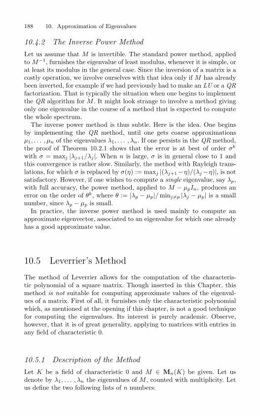
188 10. Approximation of Eigenvalues
10.4.2 The Inverse Power Method
Let us assume that M is invertible. The standard power method, appliedto M−1, furnishes the eigenvalue of least modulus, whenever it is simple, orat least its modulus in the general case. Since the inversion of a matrix is acostly operation, we involve ourselves with that idea only if M has alreadybeen inverted, for example if we had previously had to make an LU or a QRfactorization. That is typically the situation when one begins to implementthe QR algorithm for M . It might look strange to involve a method givingonly one eigenvalue in the course of a method that is expected to computethe whole spectrum.
The inverse power method is thus subtle. Here is the idea. One beginsby implementing the QR method, until one gets coarse approximationsµ1, . . . , µn of the eigenvalues λ1, . . . , λn. If one persists in the QR method,the proof of Theorem 10.2.1 shows that the error is at best of order σk
with σ = maxj |λj+1/λj |. When n is large, σ is in general close to 1 andthis convergence is rather slow. Similarly, the method with Rayleigh trans-lations, for which σ is replaced by σ(η) := maxj |(λj+1−η)/(λj−η)|, is notsatisfactory. However, if one wishes to compute a single eigenvalue, say λp,with full accuracy, the power method, applied to M − µpIn, produces anerror on the order of θk, where θ := |λp − µp|/ minj =p |λj − µp| is a smallnumber, since λp − µp is small.
In practice, the inverse power method is used mainly to compute anapproximate eigenvector, associated to an eigenvalue for which one alreadyhas a good approximate value.
10.5 Leverrier’s Method
The method of Leverrier allows for the computation of the characteris-tic polynomial of a square matrix. Though inserted in this Chapter, thismethod is not suitable for computing approximate values of the eigenval-ues of a matrix. First of all, it furnishes only the characteristic polynomialwhich, as mentioned at the opening if this chapter, is not a good techniquefor computing the eigenvalues. Its interest is purely academic. Observe,however, that it is of great generality, applying to matrices with entries inany field of characteristic 0.
10.5.1 Description of the Method
Let K be a field of characteristic 0 and M ∈ Mn(K) be given. Let usdenote by λ1, . . . , λn the eigenvalues of M , counted with multiplicity. Letus define the two following lists of n numbers:

10.5. Leverrier’s Method 189
Elementary symmetric polynomials
σ1 := λ1 + · · ·+ λn = TrM,
σ2 :=∑j<k
λjλk,
...σr :=
∑j1<···<jr
λj1 · · ·λjr ,
...σn :=
∏j
λj = detM.
Newton sums
sm :=∑
j
λmj , 1 ≤ m ≤ n.
The numbers (−1)jσj are the coefficients of the characteristic polynomialof M :
PM (X) = Xn − σ1Xn−1 + σ2X
n−2 − · · ·+ (−1)nσn.
Furthermore, the sm are the traces of the powers Mm. One can obtainthem by computing M2, . . . , Mn. Each of these matrices is obtained inO(nα) operations, with 2 ≤ α ≤ 3 (α = 3, using the naive method forthe product of two matrices). In all, the computation of s1, . . . , sn needsO(nα+1) operations, which is a lot, compared to iterative methods (QR ,Jacobi), for which each iteration is made in O(n2) operations at worst.
The passage from Newton sums to elementary symmetric polynomials isdone through Newton’s formulas. If Σj = (−1)jσj and Σ0 := 1, we have
mΣm +m∑
k=1
skΣm−k = 0, 1 ≤ n.
One uses these formulas in increasing order, beginning with Σ1 = −s1.When Σ1, . . . ,Σm−1 are known, one computes
Σm = − 1m
(s1Σm−1 + · · ·+ smΣ0).
This computation, which needs only O(n2) operations, has a negligible cost.Besides the high cost of this method, its instability is unfortunate when
k = IR or k = CC: when n is large, sk increases like ρ(M)k, thus muchmore rapidly than σk. The eigenvalues of smaller modulus are thus muchperturbed by the round-off errors, and this is reinforced by the large numberof operations.

190 10. Approximation of Eigenvalues
When the field is of nonzero characteristic p, the Leverrier method maybe employed only if n < p. Since sp = σp
1 , the computation of the sm’s form ≥ p does not bring any new information about the σj ’s.
10.6 Exercises
1. Given a polynomial P ∈ IR[X ], use the Euclidean division in order todefine a sequence of nonzero polynomials Pj in the following way. SetP0 = P , P1 = P ′. If Pj is not constant, −Pj+1 is the remainder ofthe division of Pj−1 by Pj : Pj−1 = QjPj − Pj+1, deg Pj+1 < deg Pj .
(a) Assume that P has only simple roots. Show that the sequence(Pj)j is well-defined, that it has only finitely many terms, andthat it is a Sturm sequence.
(b) Use Proposition 10.1.3 to compute the number of real roots ofthe real polynomials X2 + aX + b or X3 + pX + q in terms oftheir discriminants.
2. (J. Wilkinson [35], Section 5.45) Let n = 2p − 1 be an odd numberand Wn ∈Mn(IR) be the symmetric tridiagonal matrix
p 1
1. . .
. . .. . . 1
. . .. . . . . . 1
1 p
.
The diagonal entries are thus p, p−1, . . . , 2, 1, 2, . . . , p−1, p, and thesubdiagonal entries are equal to 1.
(a) Show that the linear subspace
E′ = X ∈ IRn |xp+j = xp−j , 1 ≤ j < pis stable under Wn. Similarly, show that the linear subspace
E′′ = X ∈ IRn |xp+j = −xp−j , 0 ≤ j < pis stable under Wn.
(b) Deduce that the spectrum of Wn is the union of the spectra ofthe matrices
W ′n =
p 1
1. . . . . .. . . . . . . . .
1 2 12 1
(∈Mp(IR))

10.6. Exercises 191
and
W ′′n =
p 1
1. . . . . .. . . . . . . . .
1 3 11 2
(∈Mp−1(IR)).
(c) Show that the eigenvalues of W ′′n separate strictly those of W ′
n.
3. For a1, . . . , an ∈ IR, with∑
j aj = 1, form the matrix
M(a) :=
a1 a2 a3 a4 an
a2 b2 a3
......
...
a3 a3 b3
......
a4 · · · ...· · · · · · an
an · · · · · · · · · an bn
,
where bj := a1 + · · ·+ aj−1 − (j − 2)aj.
(a) Compute the eigenvalues and the eigenvectors of M(a).(b) We limit ourselves to n-uplets a that belong to the simplex S
defined by 0 ≤ an ≤ · · · ≤ a1 and∑
j aj = 1. Show that fora ∈ S M(a) is bistochastic and b2 − a2 ≤ · · · ≤ bn − an ≤ 1.
(c) Let µ1, . . . , µn be an n-uplet of elements in [0, 1] with µn = 1.Show that there exists a unique a in S such that µ1, . . . , µnis equal to the spectrum of M(a) (counting with multiplicity).
(d) Consider the unit sphere Σ of Mn(IR), when this space is en-dowed with the norm ‖M‖2 =
√ρ(MT M). Show that if P ∈ Σ,
then there exists a convex polytope T , of dimension (n − 1)2,included in Σ and containing P . Hint: Use Corollary 5.5.1, withunitary invariance of the norm ‖ · ‖2.
4. Show that the cost of an iteration of the QR method for a Hermitiantridiagonal matrix is 20n + O(1).
5. Show that the reduction to the Hessenberg form (in this case,tridiagonal form) of a Hermitian matrix costs 7n3/6 + O(n2)operations.
6. (Invariants of the algorithm QR ) For M ∈Mn(IR) and 1 ≤ k ≤ n−1,let us denote by (M)k the matrix of size (n−k)× (n−k) obtained bydeleting the first k rows and the last k columns. For example, (I)1 isthe Jordan matrix J(0; n− 1). We shall denote also by K ∈Mn(IR)the matrix defined by k1n = 1 and kij = 0 otherwise.

192 10. Approximation of Eigenvalues
(a) For an upper triangular matrix T , compute explicitly KT andTK.
(b) Let M ∈Mn(IR). Prove the equality
det(M − λI − µK) = (−1)nµ det(M − λI)1 + det(M − λI).
(c) Let A ∈ GLn(IR) be given, with factorization A = QR. Provethat
det(A− λI)1 =detR
rnndet(Q− λR−1)1.
(d) Let A′ = RQ. Show that
rnn det(A′ − λI)1 = r11 det(A− λI)1.
(e) Generalize the previous calculation by replacing the index 1 byk. Deduce that the roots of the polynomial det(A − λI)k areconserved throughout the QR algorithm. How many such rootsdo we have for a general matrix? How many for a Hessenbergmatrix?
7. (Invariants; continuing) For M ∈ Mn(IR), let us define PM (h; z) :=det((1− h)M + hMT − zIn).
(a) Show that PM (h; z) = PM (1 − h; z). Deduce that there exists apolynomial QM such that PM (h; z) = QM (h(1− h); z).
(b) Show that QM remains constant throughout the QR algorithm:If Q ∈ On(IR), R is upper triangular, and M = QR, N = RQ,then QM = QN .
(c) Deduce that there exist polynomial functions Jrk on Mn(IR),defined by
PM (h; z) =n∑
r=0
[r/2]∑k=0
(h(1 − h))kzn−rJrk(M),
that are invariant throughout the QR algorithm. Verify that theJr0’s can be expressed in terms of invariants that we alreadyknow.
(d) Compute explicitly J21 when n = 2. Deduce that in the casewhere Theorem 10.2.1 applies and detA > 0, the matrix Ak
converges.(e) Show that for n ≥ 2,
J21(M) = −12
Tr((M −MT )2
).
Deduce that if Ak converges to a diagonal matrix, then A issymmetric.

10.6. Exercises 193
8. In the Jacobi method, show that if the eigenvalues are simple, thenthe product R1 · · ·Rm converges, to an orthogonal matrix R suchthat R∗AR is diagonal.
9. Extend the Jacobi method to Hermitian matrices. Hint: Replace therotation matrices (
cos θ sin θ− sin θ cos θ
)
by unitary matrices (z1 z2
z3 z4
).
10. Let A ∈ Symn(IR) be a matrix whose eigenvalues, of course real, aresimple. Apply the Jacobi method, but selecting the angle θk so thatπ/4 ≤ |θk| ≤ π/2.
(a) Show that Ek tends to zero, that the sequence Dk is relativelycompact, and that its cluster values are diagonal matrices whosediagonal terms are the eigenvalues of A.
(b) Show that an iteration has the effect of permuting, asymp-totically, a
(k)pp and a
(k)qq , where (p, q) = (pk, qk). In other
words
limk→+∞
|a(k+1)pp − a(k)
qq | = 0,
and vice versa, permuting p and q.
11. The Bernoulli method computes an approximation of the root oflargest modulus for a polynomial a0X
n + · · · + an, when that rootis unique. To do so, one defines a sequence by a linear induction oforder n:
zk = − 1a0
(a1zk−1 + · · ·+ anzk−n).
Compare this method with the power method for a suitable matrix.
12. Consider the power method for a matrix M ∈Mn(CC) of which severaleigenvalues are of modulus ρ(M) = 0. Again, CCn = E ⊕ F is thedecomposition of CCn into linear subspaces stable under M , such thatρ(M |F ) < ρ(M) and λ ∈ Sp(M |E) =⇒ |λ| = ρ(M). Finally, x0 =y0 + z0 with y0 ∈ E, z0 ∈ F , and y0 = 0.
(a) Express
1m
m−1∑k=0
log ‖Mxk‖
in terms of ‖Mmx0‖.

194 10. Approximation of Eigenvalues
(b) Show that if 0 < µ < ρ(M) < η, then there exist constants C, C′
such that
Cµk ≤ ‖Mkx0‖ ≤ C′ηk, ∀k ∈ IN.
(c) Deduce that log ‖Mxk‖ converges in the mean to log ρ(M).
13. Let M ∈ Mn(CC) be given. Assume that the Gershgorin disk Dl isdisjoint from the other disks Dm, m = l. Show that the inverse powermethod, applied to M−mllIn, provides an approximate computationof the unique eigenvalue of M that belongs to Dl.

References
[1] Jacques Baranger. Analyse numerique. Hermann, Paris, 1991.
[2] G. R. Belitskii and Yurii. I. Lyubich. Matrix norms and their applications,volume 36 of Operator theory : advances and applications. Birkhauser, Bale,1988.
[3] M. Berger and B. Gostiaux. Differential geometry : manifold, curves andsurfaces, volume 115 of Graduate text in Mathematics. Springer-Verlag, NewYork, 1988.
[4] Rajendra Bhatia. Matrix Analysis, volume 169 of Graduate text in Mathe-matics. Springer-Verlag, Heidelberg, 1996.
[5] Rajendra Bhatia. Pinching, trimming, truncating, and averaging of matrices.Amer. Math. Monthly, 107(7):602–608, 2000.
[6] Rajendra Bhatia. Linear algebra to quantum cohomology : the story ofAlfred Horn’s inequalities. Amer. Math. Monthly, 108(4):289–318, 2001.
[7] Peter Burgisser, Michael Clausen, and M. Amin Shokrollahi. Algebraiccomplexity theory. Springer-Verlag, Berlin, 1997. With the collaboration ofThomas Lickteig.
[8] Philippe Ciarlet. Introduction to numerical linear algebra and optimisa-tion. Cambridge texts in Applied Mathematics. Cambridge University Press,Cambridge, 1989.
[9] Philippe Ciarlet and Jean-Marie Thomas. Exercices d’analyse numeriquematricielle et d’optimisation. Mathematiques appliquees pour la maıtrise.Masson, Paris, 1982.
[10] Harvey Cohn. Advanced number theory. Dover Publications Inc., New York,1980. Reprint of A second course in number theory, 1962, Dover Books onAdvanced Mathematics.

196 References
[11] Don Coppersmith and Shmuel Winograd. Matrix multiplication via arith-metic progressions. J. Symbolic Comput., 9(3):251–280, 1990.
[12] J. Davis, Philip. Circulant matrices. Chelsea Publishing, New York, 1979.
[13] M. Fiedler and V. Ptak. On matrices with non-positive off-diagonal elementsand positive principal minors. Czech. Math. Journal, 12:382–400, 1962.
[14] Edward Formanek. Polynomial identities and the Cayley-Hamilton theorem.Math. Intelligencer, 11(1):37–39, 1989.
[15] Edward Formanek. The polynomial identities and invariants of n × n ma-trices. Number 78 in CBMS Regional Conf. Ser. Math. Amer. Math. Soc.,Providence, RI, 1991.
[16] William Fulton. Eigenvalues, invariant factors, highest weights, and Schubertcalculus. Bull. Amer. Math. Soc. (N.S.), 37(3):209–249 (electronic), 2000.
[17] F. R. Gantmacher. The theory of matrices. Vol. 1. Chelsea Publish. Co.,New York, 1959.
[18] F. R. Gantmacher. The theory of matrices. Vol. 2. Chelsea Publish. Co.,New York, 1959.
[19] Gene H. Golub and Charles F. Van Loan. Matrix computations, volume 3of Series in the mathematical sciences. John Hopkins University Press,Baltimore, 1983.
[20] Nicholas Higham. Accuracy and stability of numerical algorithms. SIAM,Philadelphia, PA, 1996.
[21] Roger A. Horn and Charles R. Johnson. Matrix analysis. CambridgeUniversity Press, Cambridge, 1985.
[22] Alston S. Householder. The theory of matrices in numerical analysis. Dover,New York, 1975.
[23] Nicholas M. Katz and Peter Sarnak. Random matrices, Frobenius eigenval-ues and monodromy. Number 45 in Colloquium publ. Amer. Math. Soc.,Providence, RI, 1999.
[24] Anthony W. Knapp. Representation of semisimple groups. An overview basedon examples. Princeton Mathematical Series. Princeton University Press,Princeton, NJ, 1986.
[25] P. Lascaux and R. Theodor. Analyse numerique matricielle appliquee a l’artde l’ingenieur. Masson, Paris, 1987.
[26] Chi-Wang Li and Roy Mathias. Extremal characterization of the Schurcomplement and resulting inequalities. SIAM Review, 42:233–246, 2000.
[27] Helmut Lutkepohl. Handbook of matrices. J. Wiley & Sons, New York, 1996.
[28] Mneimne, Rached and Testard, Frederic. Introduction a la theorie desgroupes de Lie classiques. Hermann, Paris, 1986.
[29] Walter Rudin. Real and complex analysis. McGraw-Hill Book co, NY, thirdedition, 1987.
[30] Walter Rudin. Functional analysis. McGraw-Hill Book Co, NY, secondedition, 1991.
[31] E. Seneta. Non-negative matrices and Markov chains. Springer series instatistics. Springer-Verlag, New York-Berlin, 1981.

References 197
[32] Joseph Stoer and Christoph Witzgall. Transformations by diagonal matricesin a normed space. Numer. Math., 4:158–171, 1962.
[33] Volker Strassen. Gaussian elimination is not optimal. Numer. Math., 13:354–356, 1969.
[34] J. H. M. Wedderburn. Lectures on matrices, volume XVII of Colloquiumpublications. American Math. Society, New York, 1934.
[35] J. H. Wilkinson. The algebraic eigenvalue problem. Oxford Science Publica-tions, Oxford, 1965.

This page intentionally left blank

Index
QRfactorization, 143method, 173
algebraBanach, 70Lie, 134
algebraically closed field, 4
Abeltheorem, 110, 168
algebranormed, 70
alternateform, 12matrix, 11
Amitsur & Levitzkitheorem, 38
basis, 2
Campbell–Hausdorffformula, 134
canonical form, 107, 110Cauchy–Binet
formula, 18Cayley–Hamilton
theorem, 26characteristic
of a field, 1characteristic polynomial, 24Choleski
factorization, 142cofactor, 17commutator, 6condition number, 162, 169conjugate
exponents, 62gradient, 159matrices, 9
convergence rate, 164convergence ratio, 151convergent
method, 150Cotlar
lemma, 77
determinant, 16diagonalizable
orthogonally, 48diagonally
dominant, 73strictly dominant, 73strongly dominant, 73

200 Index
domainEuclidean, 99principal ideal, 97
eigenbasis, 28eigenspace, 28eigenvalue, 24
multiplicityalgebraic, 25geometric, 25
semi-simple, 27simple, 25
eigenvector, 24elementary divisor, 109equivalent
matrices, 8norms, 63
exponential, 116extremal point, 79extreme point, 88
formHermitian, 41sesquilinear, 41
Frobeniusnorm, 182
Gaussmethod, 149
Gauss–Seidelmethod, 152
gcd, 98Gershgorin
disk, 71, 78domain, 71
Grevillealgorithm, 148
grouplinear, 20modular, 56orthochronous Lorentz, 127orthogonal, 20, 120
special, 20special linear, 20special orthogonal, 123symmetric, 15symplectic, 120topological, 135unitary, 120
Hessenberg, 169Householder
matrix, 171method, 175theorem, 67
ideal, 97principal, 97
inequalityCauchy–Schwarz, 63Holder, 62Minkowski, 61
integral domain, 15invariant factor, 102inverse
generalized, 145left, 145right, 145
irreducibility, 30
Jacobiidentity, 134method, 151, 181
Jordanblock, 110decomposition, 111
kernel, 7
Lp(Ω), 68
matricescommuting, 6conjugate, 9equivalent, 8product of, 6similar, 9
matrixHouseholder, 171Jordan, 110Pascal’s, 130adjoint, 17alternate, 11companion, 37, 106cyclic, 85diagonal, 5
block-, 10diagonalizable, 28elementary, 100

Index 201
Hermitian, 40positive definite, 42
Hermitian adjoint, 40Hessenberg, 169idempotent, 6identity, 5
inverse, 20invertible, 20nilpotent, 6
nonnegative, 80nonsingular, 20normal, 40orthogonal, 10
orthostochastic, 89permutation, 5projection, 32regular, 20
singular, 20skew-Hermitian, 40skew-symmetric, 10square, 5
stochastic, 87bi-, 87
symmetric, 10
positive definite, 42totally positive, 35transposed, 10triangular, 5
block-, 10strictly, 5
tridiagonal, 155unitary, 41
methodQR , 173power
inverse, 188conjugate gradient, 159Gauss–Seidel, 152Jacobi, 151, 181
Leverrier, 188power, 185relaxation, 152
minimal polynomial, 27
minor, 17leading principal, 17principal, 17, 137
Moore–Penrose
inverse, 145
normlp, 61algebra, 65, 70Frobenius, 182induced, 65matrix, 65Schur, 131Schur’s, 59, 182subordinated, 65
normsequivalent, 63
orthogonalgroup, 20, 120subspace, 11
orthogonallydiagonalizable, 48
Perron–Frobeniustheorem, 81, 82
Pfaffian, 22polar decomposition, 115polynomial
invariant, 104standard, 38
preconditioning, 165product
Hadamard, 59of matrices, 6scalar, 11
projector, 32
range, 7, 8rank, 5
decomposition, 104Rayleigh
ratio, 48translation, 180
reductibility, 30relaxation
method, 152residue, 160Rieszthorin
theorem, 68ring
factorial, 99Noetherian, 98principal ideal domain, 97

202 Index
Schurcomplement, 50, 139lemma, 33norm, 182theorem, 45
signature, 48similar
matrices, 9unitarily, 45
similarity invariant, 25, 104singular value, 75, 128spectral radius, 61spectrum, 24square root, 115Strassen
algorithm, 142Sturm
sequence, 173Sylvester index, 48symmetric group, 15symplectic
group, 120
trace, 25
unitarilysimilar, 45
unitarydiagonalization, 46group, 120trigonalization, 45
Vandermondematrix, 35
vectorcolumn, 5nonnegative, 80positive, 80row, 5
vector space, 2