MATLAB Tutorial Course

A.H. Taherinia

Matlab Environment

Contents Continued

Desktop toolsmatricesLogical &Mathematical operationsHandle Graphics

1

MATLAB Desktop Tools

Command WindowCommand HistoryHelp BrowserWorkspace BrowserEditor/Debugger

2

3

Calculations at the Command Line

» a = 2;

» b = 5;

» a^b

ans =

32

» x = 5/2*pi;

» y = sin(x)

y =

1

» z = asin(y)

z =

1.5708

» a = 2;

» b = 5;

» a^b

ans =

32

» x = 5/2*pi;

» y = sin(x)

y =

1

» z = asin(y)

z =

1.5708

Results assigned to “ans” if name not specified

() parentheses for function inputs

Semicolon suppresses screen output

MATLAB as a calculator Assigning Variables

A Note about Workspace:Numbers stored in double-precision floating point format

» -5/(4.8+5.32)^2ans =

-0.0488» (3+4i)*(3-4i)ans =

25» cos(pi/2)ans =6.1230e-017

» exp(acos(0.3))ans =

3.5470

» -5/(4.8+5.32)^2ans =

-0.0488» (3+4i)*(3-4i)ans =

25» cos(pi/2)ans =6.1230e-017

» exp(acos(0.3))ans =

3.5470

4

General Functionswhos: List current variablesclear: Clear variables and functions from memoryClose: Closes last figurescd: Change current working directorydir: List files in directoryecho: Echo commands in M-filesformat: Set output format

5

Matlab Help

6

Getting helphelp command (>>help)

lookfor command (>>lookfor)

Help Browser (>>doc)

helpwin command (>>helpwin)

Search EnginePrintable Documents

“Matlabroot\help\pdf_doc\”Link to The MathWorks

7

Matrices

Entering and Generating MatricesConcatenationDeleting Rows and ColumnsArray ExtractionMatrix and Array Multiplication

8

» a=[1 2;3 4]

a =

1 2

3 4

» b=[-2.8, sqrt(-7), (3+5+6)*3/4]

b =

-2.8000 0 + 2.6458i 10.5000

» b(2,5) = 23

b =

-2.8000 0 + 2.6458i 10.5000 0 0

0 0 0 0 23.0000

» a=[1 2;3 4]

a =

1 2

3 4

» b=[-2.8, sqrt(-7), (3+5+6)*3/4]

b =

-2.8000 0 + 2.6458i 10.5000

» b(2,5) = 23

b =

-2.8000 0 + 2.6458i 10.5000 0 0

0 0 0 0 23.0000

• Any MATLAB expression can be entered as a matrix element• Matrices must be rectangular. (Set undefined elements to zero)

Entering Numeric Arrays

Row separatorsemicolon (;)

Column separatorspace / comma (,)

Use square brackets [ ]

9

The Matrix in MATLAB

4 10 1 6 2

8 1.2 9 4 25

7.2 5 7 1 11

0 0.5 4 5 56

23 83 13 0 10

1

2

Rows (m) 3

4

5

Columns(n)

1 2 3 4 51 6 11 16 21

2 7 12 17 22

3 8 13 18 23

4 9 14 19 24

5 10 15 20 25

A = A (2,4)

A (17)

Rectangular Matrix:Scalar: 1-by-1 arrayVector: m-by-1 array

1-by-n arrayMatrix: m-by-n array

10

» w=[1 2;3 4] + 5w =

6 78 9

» x = 1:5

x =1 2 3 4 5

» y = 2:-0.5:0

y = 2.0000 1.5000 1.0000 0.5000 0

» z = rand(2,4)

z =

0.9501 0.6068 0.8913 0.45650.2311 0.4860 0.7621 0.0185

» w=[1 2;3 4] + 5w =

6 78 9

» x = 1:5

x =1 2 3 4 5

» y = 2:-0.5:0

y = 2.0000 1.5000 1.0000 0.5000 0

» z = rand(2,4)

z =

0.9501 0.6068 0.8913 0.45650.2311 0.4860 0.7621 0.0185

Scalar expansion

Creating sequences:colon operator (:)

Utility functions for creating matrices.

Entering Numeric Arrays

11

Numerical Array Concatenation» a=[1 2;3 4]

a =

1 2

3 4

» cat_a=[a, 2*a; 3*a, 4*a; 5*a, 6*a]cat_a =

1 2 2 43 4 6 83 6 4 89 12 12 165 10 6 12

15 20 18 24

» a=[1 2;3 4]

a =

1 2

3 4

» cat_a=[a, 2*a; 3*a, 4*a; 5*a, 6*a]cat_a =

1 2 2 43 4 6 83 6 4 89 12 12 165 10 6 12

15 20 18 24

Use [ ] to combine existing arrays as matrix “elements”

Row separator:semicolon (;)

Column separator:space / comma (,)

Use square brackets [ ]

Note:The resulting matrix must be rectangular

4*a

12

Deleting Rows and Columns » A=[1 5 9;4 3 2.5; 0.1 10 3i+1]

A =

1.0000 5.0000 9.0000

4.0000 3.0000 2.5000

0.1000 10.0000 1.0000+3.0000i

» A(:,2)=[]

A =

1.0000 9.0000

4.0000 2.5000

0.1000 1.0000 + 3.0000i

» A(2,2)=[]

??? Indexed empty matrix assignment is not allowed.

» A=[1 5 9;4 3 2.5; 0.1 10 3i+1]

A =

1.0000 5.0000 9.0000

4.0000 3.0000 2.5000

0.1000 10.0000 1.0000+3.0000i

» A(:,2)=[]

A =

1.0000 9.0000

4.0000 2.5000

0.1000 1.0000 + 3.0000i

» A(2,2)=[]

??? Indexed empty matrix assignment is not allowed.

13

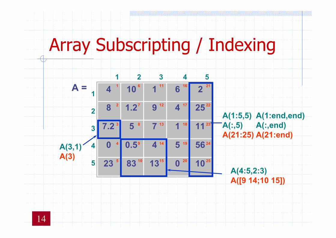
Array Subscripting / Indexing

4 10 1 6 2

8 1.2 9 4 25

7.2 5 7 1 11

0 0.5 4 5 56

23 83 13 0 10

1

2

3

4

5

1 2 3 4 51 6 11 16 21

2 7 12 17 22

3 8 13 18 23

4 9 14 19 24

5 10 15 20 25

A =

A(3,1)A(3)

A(1:5,5)A(:,5) A(21:25)

A(4:5,2:3)A([9 14;10 15])

A(1:end,end) A(:,end)A(21:end)’

14

Matrix Multiplication» a = [1 2 3 4; 5 6 7 8];

» b = ones(4,3);

» c = a*b

c =

10 10 1026 26 26

» a = [1 2 3 4; 5 6 7 8];

» b = ones(4,3);

» c = a*b

c =

10 10 1026 26 26

[2x4][4x3]

[2x4]*[4x3] [2x3]

a(2nd row).b(3rd column)

» a = [1 2 3 4; 5 6 7 8];

» b = [1:4; 1:4];

» c = a.*b

c =

1 4 9 165 12 21 32

» a = [1 2 3 4; 5 6 7 8];

» b = [1:4; 1:4];

» c = a.*b

c =

1 4 9 165 12 21 32 c(2,4) = a(2,4)*b(2,4)

Array Multiplication

15

Matrix Manipulation Functions• zeros: Create an array of all zeros• ones: Create an array of all ones• eye: Identity Matrix• rand: Uniformly distributed random numbers• diag: Diagonal matrices and diagonal of a matrix• size: Return array dimensions

16

Matrix Manipulation Functions• transpose (’): Transpose matrix• rot90: rotate matrix 90• tril: Lower triangular part of a matrix• triu: Upper triangular part of a matrix• cross: Vector cross product• dot: Vector dot product• det: Matrix determinant• inv: Matrix inverse • rank: Rank of matrix

17

Elementary Math

Logical Operators

Math Functions

18

Logical Operations» Mass = [-2 10 NaN 30 -11 Inf 31];» each_pos = Mass>=0each_pos =

0 1 0 1 0 1 1» all_pos = all(Mass>=0)all_pos =

0» all_pos = any(Mass>=0)all_pos =

1» pos_fin = (Mass>=0)&(isfinite(Mass))pos_fin =

0 1 0 1 0 0 1

» Mass = [-2 10 NaN 30 -11 Inf 31];» each_pos = Mass>=0each_pos =

0 1 0 1 0 1 1» all_pos = all(Mass>=0)all_pos =

0» all_pos = any(Mass>=0)all_pos =

1» pos_fin = (Mass>=0)&(isfinite(Mass))pos_fin =

0 1 0 1 0 0 1

= = equal to> greater than

< less than

>= Greater or equal

<= less or equal

~ not

& and

| or

isfinite(), etc. . . .

all(), any()

find

Note:• 1 = TRUE• 0 = FALSE

19

Elementary Math Function• abs, sign: Absolute value and Signum Function• sin, cos, asin, acos…: Triangular functions• exp, log, log10: Exponential, Natural and

Common (base 10) logarithm• ceil, floor: Round toward infinities• fix: Round toward zero

20

Elementary Math Functionround: Round to the nearest integergcd: Greatest common devisorlcm: Least common multiplesqrt: Square root functionreal, imag: Real and Image part of

complexrem: Remainder after division

21

Elementary Math Function• max, min: Maximum and Minimum of arrays• mean, median: Average and Median of arrays• std, var: Standard deviation and variance• sort: Sort elements in ascending order• sum, prod: Summation & Product of Elements

22

Graphics Fundamentals

23

GraphicsBasic Plotting

plot, title, xlabel, grid,legend, hold, axis

Editing PlotsProperty Editor

24

2-D PlottingSyntax:

Example:plot(x1, y1, 'clm1', x2, y2, 'clm2', ...)plot(x1, y1, 'clm1', x2, y2, 'clm2', ...)

x=[0:0.1:2*pi];y=sin(x);z=cos(x);plot(x,y,x,z,'fontsize',14);legend('Y data','Z data ,'linewidth',2)title('Sample Plot','fontsize',14);xlabel('X values','fontsize',14);ylabel('Y values','fontsize',14);grid on

x=[0:0.1:2*pi];y=sin(x);z=cos(x);plot(x,y,x,z,'fontsize',14);legend('Y data','Z data ,'linewidth',2)title('Sample Plot','fontsize',14);xlabel('X values','fontsize',14);ylabel('Y values','fontsize',14);grid on

25

Sample PlotTitle

Ylabel

Xlabel

Grid

Legend

26

Subplot

subplot(m,n,p)

income = [3.2 4.1 5.0 5.6];outgo = [2.5 4.0 3.35 4.9];subplot(2,1,1); plot(income);subplot(2,1,2); plot(outgo);

income = [3.2 4.1 5.0 5.6];outgo = [2.5 4.0 3.35 4.9];subplot(2,1,1); plot(income);subplot(2,1,2); plot(outgo);

27

Subplot

28

Subplot

subplot(m,n,p)

income = [3.2 4.1 5.0 5.6];outgo = [2.5 4.0 3.35 4.9];subplot(2,2,[1 3]); plot(income);subplot(2,2,2); plot(outgo);subplot(2,2,4); plot(income+outgo);

income = [3.2 4.1 5.0 5.6];outgo = [2.5 4.0 3.35 4.9];subplot(2,2,[1 3]); plot(income);subplot(2,2,2); plot(outgo);subplot(2,2,4); plot(income+outgo);

29

Subplot

30

SubplotsSyntax:

»subplot(2,2,1); » …

»subplot(2,2,2)» ...

»subplot(2,2,3)» ...

»subplot(2,2,4)» ...

»subplot(2,2,1); » …

»subplot(2,2,2)» ...

»subplot(2,2,3)» ...

»subplot(2,2,4)» ...

subplot(rows,cols,index)subplot(rows,cols,index)

31

Programming andApplication Development

32

Script and Function Files• Script Files

• Work as though you typed commands into MATLAB prompt

• Variable are stored in MATLAB workspace

• Function Files• Let you make your own MATLAB Functions• All variables within a function are local• All information must be passed to functions as

parameters• Sub functions are supported

33

Basic Parts of a Function M-File

function y = mean (x)% MEAN Average or mean value.% For vectors, MEAN(x) returns the mean value.% For matrices, MEAN(x) is a row vector% containing the mean value of each column.[m,n] = size(x);if m == 1

m = n;endy = sum(x)/m;

Output Arguments Input ArgumentsFunction Name

Online Help

Function Code

34

eps = 1;

while (1+eps) > 1

eps = eps/2;

end

eps = eps*2

eps = 1;

while (1+eps) > 1

eps = eps/2;

end

eps = eps*2

while Loops

Flow Control Statements

35

a = zeros(k,k) % Preallocate matrix

for m = 1:k

for n = 1:k

a(m,n) = 1/(m+n -1);

end

end

a = zeros(k,k) % Preallocate matrix

for m = 1:k

for n = 1:k

a(m,n) = 1/(m+n -1);

end

end

for Loop

method = 'Bilinear';

switch lower(method)

case {'linear','bilinear'}

disp('Method is linear')

case 'cubic'

disp('Method is cubic')

otherwise

disp('Unknown method.')

end

Method is linear

method = 'Bilinear';

switch lower(method)

case {'linear','bilinear'}

disp('Method is linear')

case 'cubic'

disp('Method is cubic')

otherwise

disp('Unknown method.')

end

Method is linear

Switch Statement

Flow Control Statements

36

if ((attendance >= 0.90) & (grade_average >= 60))

pass = 1;

end;

if ((attendance >= 0.90) & (grade_average >= 60))

pass = 1;

end;

if Statement

Function M-file

function r = ourrank(X,tol)% rank of a matrixs = svd(X);if (nargin == 1)

tol = max(size(X)) * s(1)* eps;endr = sum(s > tol);

function r = ourrank(X,tol)% rank of a matrixs = svd(X);if (nargin == 1)

tol = max(size(X)) * s(1)* eps;endr = sum(s > tol);

function [mean,stdev] = ourstat(x)[m,n] = size(x);if m == 1

m = n;endmean = sum(x)/m;stdev = sqrt(sum(x.^2)/m – mean.^2);

function [mean,stdev] = ourstat(x)[m,n] = size(x);if m == 1

m = n;endmean = sum(x)/m;stdev = sqrt(sum(x.^2)/m – mean.^2);

Multiple Input Argumentsuse ( )

Multiple Output Arguments, use [ ]

»r=ourrank(rand(5),.1);

»[m std]=ourstat(1:9);

37

38

Image Processing Toolbox

Introduction

Collection of functions (MATLAB files) that supports a wide range of image processing operations

Image Coordinate

Read an ImageRead in an imageValidates the graphic format

(bmp, hdf, jpeg, pcx, png, tiff, xwd)

Store it in an arrayclear, close all;I = imread(‘pout.tif`);[X, map] = imread(‘pout.tif’);

Display an Imageimshow(I)

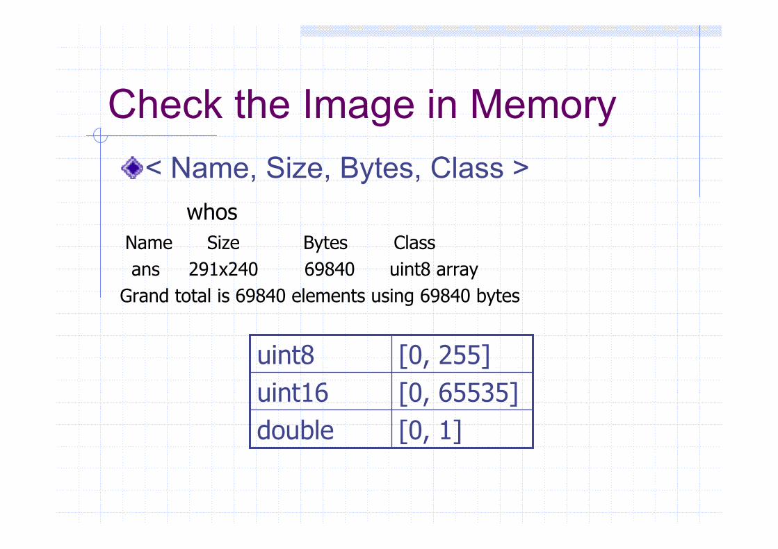
Check the Image in Memory< Name, Size, Bytes, Class >

whosName Size Bytes Classans 291x240 69840 uint8 array

Grand total is 69840 elements using 69840 bytes

[0, 1]double[0, 65535]uint16[0, 255]uint8

Data Classes

Convert between image Classes

Histogram EqualizationHistogram: distribution of intensities

figure, imhist(I)

Equalize Image (contrast)I2 = histeq(I);

figure, imshow(I2)figure, imhist(I2)

Histogram Equalization (cont.)

Histogram Equalization (cont.)

Write the Image

Validates the extensionWrites the image to disk

imwrite(I2, ’pout2.png’);imwrite(I2, ‘pout2.png’, ‘BitDepth’, 4);

Filtering Using imfilter

Filtering of images, either by correlation or convolution, can be performed using the toolbox function imfilter.

This example filters an image with a 5-by-5 filter containing equal weights. Such a filter is often called an averaging averaging filterfilter..

Filtering Using imfilterI = imread('coins.png');h = ones(5,5) / 25;I2 = imfilter(I,h);imshow(I), title('Original Image');figure, imshow(I2), title('Filtered Image')

Create special 2-D filters

h = fspecial(type) creates a two-dimensional filter h of the specified type.

Syntaxh = fspecial(type)h = fspecial(type,parameters)

Create special 2-D filters

Using Median Filtering

Median filtering is similar to using an averaging filter, in that each output pixel is set to an average of the pixel values in the neighborhood of the corresponding input pixel.

B = medfilt2(A,[m n])B = medfilt2(A)B = medfilt2(A,'indexed',...)

Using Median Filtering

I = imread('eight.tif');subplot(2,2,1), imshow(I), title('Original image');J = imnoise(I,'salt & pepper',0.02);subplot(2,2,2), imshow(J), title('Salt & pepper noise add');K = imfilter(J, fspecial('average',3));subplot(2,2,3), imshow(K), title('averaging filter');L = medfilt2(J,[3 3]);subplot(2,2,4), imshow(L), title('median filter');

Median Filtering

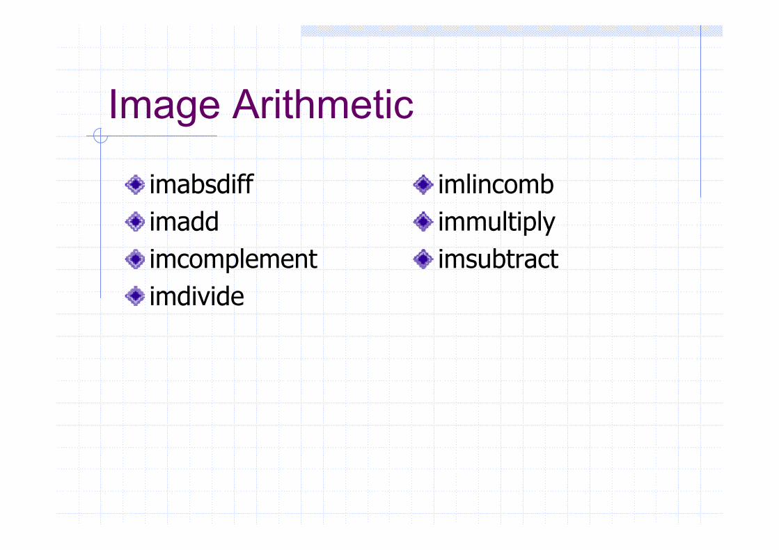
Image Arithmetic

imabsdiffimaddimcomplementimdivide

imlincombimmultiplyimsubtract

Adding Images

X = uint8([ 255 0 75; 44 225 100]);Y = uint8([ 50 50 50; 50 50 50 ]);Z = imadd(X,Y)Z =

255 50 125 94 255 150

Adding Images (cont.)I = imread(‘rice.tif’);

J = imread(‘cameraman.tif’);K = imadd(I, J);imshow(K)

Adding Images (cont.)Brighten an image results saturation

RGB = imread(‘flowers.tif’);RGB2 = imadd(RGB, 50);subplot(1, 2, 1); imshow(RGB);subplot(1, 2, 2); imshow(RGB2);

Subtracting Images

Background of a scenerice = imread(‘rice.tif’);background = imopen(rice, strel(‘disk’, 15));rice2 = imsubtract(rice, background);imshow(rice), figure, imshow(rice2);

Negative valuesimabsdiff

Subtracting Images (cont.)

Multiplying Images

Scaling: multiply by a constant(brightens >1, darkens <1)

Preserves relative contrastI = imread(‘moon.tif’);J = immultiply(I, 1.2);imshow(I);figure, imshow(J)

Multiplying Images (cont.)

Dividing Images (Ratioing)I = imread('rice.png'); J = imdivide(I,2);subplot(1,2,1), imshow(I)subplot(1,2,2), imshow(J)

Spatial Transformations

Map pixel locations in an input image to new locations in an output image

ResizingRotationCropping

Resizing Images

Change the size of an imageI = imread(‘ic.tif’); J = imresize(I, 1.25);K = imresize(I, [100 150]);figure, imshow(J)figure, imshow(K)

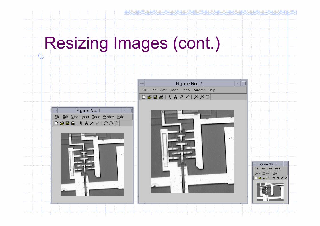
Resizing Images (cont.)

Rotating Images

Rotate an image by an angle in degreesI = imread(‘ic.tif’); J = imrotate(I, 35, ‘bilinear’);imshow(I)figure, imshow(J)

Rotating Images (cont.)

Cropping Images

Extract a rectangular portion of an image

imshow ic.tifI = imcrop;

GUIDE

GUIDE:Graphical User Interface Design Environment

GUIDE

Morphological Opening

Remove objects that cannot completely contain a structuring element

Estimate background illuminationclear, close allI = imread(‘rice.png’);imshow(I)background = imopen(I, strel(‘disk’, 15));imshow(background)

Morphological Opening (cont.)

Subtract Images

Create a more uniform backgroundI2 = imsubtract(I, background);figure, imshow(I2)

Adjust the Image Contrast

stretchlim computes [low hight] to be mapped into [bottom top]

I3 = imadjust(I2, stretchlim(I2), [0 1]);figure, imshow(I3)

Apply Thresholding to the Image

Create a binary thresholded image1. Compute a threshold to convert the intensity

image to binary2. Perform thresholding creating a logical matrix

(binary image)level = graythresh(I3);bw = im2bw(I3, level);figure, imshow(bw)

Apply Thresholding to the Image (cont.)

Labeling Connected Components

Determine the number of objects in the imageAccuracy

(size of objects, approximated background, connectivity parameter, touching objects)

[labeled, numObjects] = bwlabel(bw, 4);numObjects {= 80}

max(labeled(:))

Select and Display Pixels in a Region

Interactive selectiongrain = imcrop(labeled)

Colormap creation functionRGB_label = label2rgb(labeled,

@spring, ‘c’, ‘shuffle’);imshow(RGB_label);rect = [15 25 10 10];roi = imcrop(labeled, rect)

Object Properties

Measure object or region propertiesgraindata = regionprops(labeled, ‘basic’)graindata(51).Area {296}graindata(51).BoundingBox {142.5 89.5 24.0 26.0}graindata(51).Centroid {155.3953 102.1791}

Create a vector which holds just one property for each object

allgrains = [graindata.Area];whos

Statistical Properties of Objects

max(allgrains) { 695 }

Return the component label of a grain size

biggrain = find(allgrains == 695) { 68 }

Mean grain sizemean(allgrains) { 249 }

Histogram (#bins)hist(allgrains, 20)

Statistical Properties of Objects (cont.)

Storage Classes

double (64-bit), uint8 (8-bit), and uint16 (16-bit)

Converting (rescale or offset)doubleim2double (automatic rescale and offsetting)RGB2 = im2uint8(RGB1);im2uint16imapprox (reduce number of colors: indexed images)

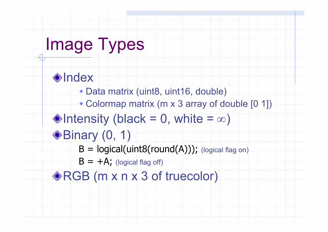
Image Types

IndexData matrix (uint8, uint16, double)Colormap matrix (m x 3 array of double [0 1])

Intensity (black = 0, white = ∞)Binary (0, 1)

B = logical(uint8(round(A))); (logical flag on)

B = +A; (logical flag off)

RGB (m x n x 3 of truecolor)

Converting Image Types

dithergray2indgraysliceim2bwind2gray

ind2rgbmat2grayrgb2grayrgb2ind

Multiframe Image Arrays

Same size, #planes, colormapStore separate images into one multiframe array

A = cat(4, A1, A2, A3, A4, A5)

Extract frames from a multiframe arrayFRM3 = MULTI(:, :, :, 3)

Display a frameimshow(MULTI(:, :, :, 7))

Coordinate Systems

Pixel CoordinatesDiscrete unit (integer)(r, c)⎡ = (1, 1)

Spatial CoordinatesContinuous unit(x, y)⎡= (0.5, 0.5)

123

Non-default Spatial Coordinate System

A = magic(5);x = [19.5 23.5];y = [8.0 12.0];image(A, ‘xData’, x, ‘yData’, y), axis image, colormap(jet(25))