MATLAB TutorialAmir massoud Farahmand

http://www.cs.ualberta.ca/~amir

Introduction to Matlab

Ela P !ekalska, Marjolein van der Glas

Pattern Recognition Group, Faculty of Applied Sciences

Delft University of Technology

January 2002

Send comments to ela@ph.tn.tudelft.nl

Version 0.6: September 24, 2008

[CMPUT 651] Probabilistic Graphical ModelsRuss Greiner and Matt Brown

The MATLAB logo is a trademark of MathWorks, Inc.

What is MATLAB?

• A scripting/programming language for numerical calculations

• Pros

• Fast prototyping for your [numerical] algorithms

• Drawing graphs easily

• Fast matrix computation

• Cons

• Slow for many other things (e.g. for loops are terribly slow)

• Not a general-purpose programming language

• Not so cheap

How to Run MATLAB@ U of A?

login to bonanza, pipestone, eureka, etc.

or matlab -nodesktop

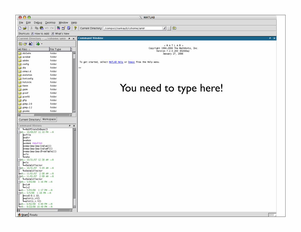
You need to type here!

I Will Talk About ...

• vectors and matrices in MATLAB

• several useful predefined functions

• graphics

• writing your own functions

• tricks for writing efficient codes

• ...

Vectors>> a = 2

a =

2

>> b = [1 2 3]

b =

1 2 3

>> c = [-1 1.1 2]'

c =

-1.0000 1.1000 2.0000

>> a = 2

a =

2

>> b = [1 2 3]

b =

1 2 3

>> c = [-1 1.1 2]'

c =

-1.0000 1.1000 2.0000

>> a*b

ans =

2 4 6

>> c*b

ans =

-1.0000 -2.0000 -3.0000 1.1000 2.2000 3.3000 2.0000 4.0000 6.0000

>> b*c

ans =

7.2000

Vectors

>> a = 2

a =

2

>> b = [1 2 3]

b =

1 2 3

>> c = [-1 1.1 2]'

c =

-1.0000 1.1000 2.0000

>> a*b

ans =

2 4 6

>> c*b

ans =

-1.0000 -2.0000 -3.0000 1.1000 2.2000 3.3000 2.0000 4.0000 6.0000

>> b*c

ans =

7.2000

>> sin(b)

ans =

0.8415 0.9093 0.1411

>> exp(c)

ans =

0.3679 3.0042 7.3891

>> b + c??? Error using ==> plusMatrix dimensions must agree.

>> b + c'

ans =

0 3.1000 5.0000

Vectors

>> x = -2*pi:0.01:2*pi;>> y = sin(x);>> y2 = sin(x) + cos(2*x) + 0.1*sin(10*x);>> plot(x,y,'b')>> holdCurrent plot held>> plot(x,y2,'k')

Another way to generate vectors

>> x = -2*pi:0.01:2*pi;>> y = sin(x);>> y2 = sin(x) + cos(2*x) + 0.1*sin(10*x);>> plot(x,y,'b')>> holdCurrent plot held>> plot(x,y2,'k')xlabel('Time'); ylabel('Amplitude'); title('My sinusoid wave')

Matrices>> A = [1 2 3;4 5 6]

A =

1 2 3 4 5 6

>> B = ones(3,5)

B =

1 1 1 1 1 1 1 1 1 1 1 1 1 1 1

>> C = zeros(3)

C =

0 0 0 0 0 0 0 0 0

Matrices>> A = [1 2 3;4 5 6]

A =

1 2 3 4 5 6

>> B = ones(3,5)

B =

1 1 1 1 1 1 1 1 1 1 1 1 1 1 1

>> C = zeros(3)

C =

0 0 0 0 0 0 0 0 0

>> D = A*B

D =

6 6 6 6 6 15 15 15 15 15

size(D)

ans =

2 5

Accessing Elements of Vectors and Matrices

a = [1 2 3 4 5 6 7 8 9 10]

a =

1 2 3 4 5 6 7 8 9 10

a(3)

ans =

3

A = [1 2 3 4;5 6 7 8; 9 10 11 12;13 14 15 16]

A =

1 2 3 4 5 6 7 8 9 10 11 12 13 14 15 16

>> B = A(2:3,2:4)

B =

6 7 8 10 11 12

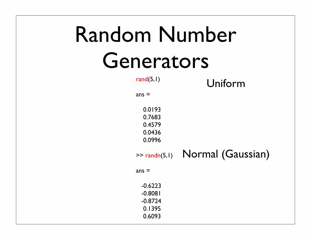
Random Number Generators

rand(5,1)

ans =

0.0193 0.7683 0.4579 0.0436 0.0996

>> randn(5,1)

ans =

-0.6223 -0.8081 -0.8724 0.1395 0.6093

Uniform

Normal (Gaussian)

Random Numbers and Histograms

X1 = randn(2000,1);>> X2 = rand(2000,1);>> hist(X1,20)

sums, means, var X = randn(1000,1);>> Y = rand(1000,1);>> sum(X), mean(X), var(X)

ans = -14.6247ans = -0.0146ans = 1.0325>> sum(Y), mean(Y), var(Y)ans = 491.2878ans = 0.4913ans = 0.0863

min(X), max(X)

ans = -3.5851ans = 3.7476>> min(Y), max(Y)ans = 0.0010ans = 0.9973

Matrices Again!A = [1 2 3; 4 5 6; 7 8 9]A =

1 2 3 4 5 6 7 8 9>> B = [1 -1 1;1 0 0;0 1 1]B =

1 -1 1 1 0 0 0 1 1>> rank(A)ans = 2>> eig(A)ans =

16.1168 -1.1168 -0.0000

A*Bans =

3 2 4 9 2 10 15 2 16

>> A.*Bans =

1 -2 3 4 0 0 0 8 9B./Aans =

1.0000 -0.5000 0.3333 0.2500 0 0 0 0.1250 0.1111

How to Write a Program?

• Script

• Anything that you do in command line except in a single file

• Functions

• Get inputs, return outputs

MATLAB forMachine Learning: Regression

Assume that y = f(x) + ! where E{!} = 0. The goal is estimating theregressor, f(.), using samples {(Xi, Yi)}, i = 1, · · · , n.There are books written on this topic, but for now, we consider a simple (bute!cient) method called Kernel regression estimator.

Let h > 0 be a positive number called the bandwidth. The Nadaraya-Watsonkernel estimator is defined by

f̂(x) =1

!nj=1 K

"x!xj

h

#n$

i=1

K

%x! xi

h

&Yi

Kernels can have di!erent forms. An example of them is Gaussian kernel:

K(x) =1!2!

exp("x2/2).

See L. Wasserman, All of Nonparametric Statistics (Section 5.4) for more information.

Let’s implement it!

What Do We Need?

• Some function f(x)

• Noisy samples from f(x)

• Kernel regressor

• kernel function (e.g. Gaussian)

A Script File as the Skeleton of the Program

edit KernelRegressionTest

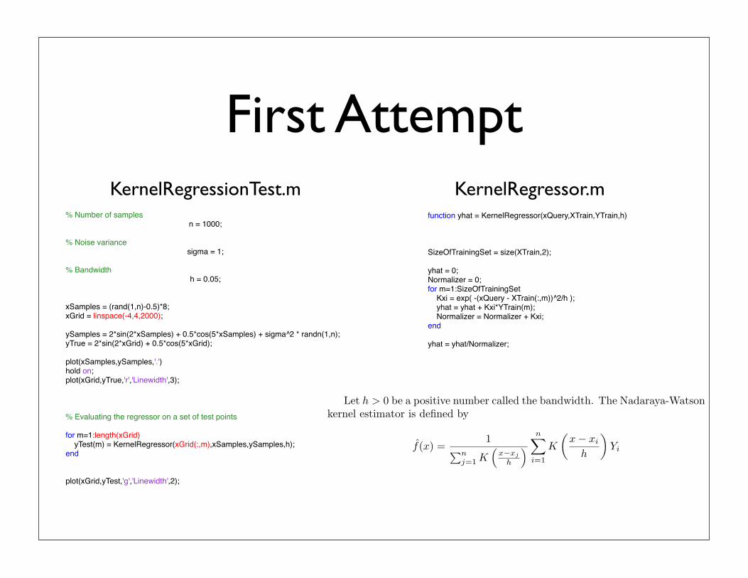
First Attempt

% Number of samplesn = 1000;

% Noise variance

sigma = 1;

% Bandwidthh = 0.05;

xSamples = (rand(1,n)-0.5)*8;xGrid = linspace(-4,4,2000); ySamples = 2*sin(2*xSamples) + 0.5*cos(5*xSamples) + sigma^2 * randn(1,n);yTrue = 2*sin(2*xGrid) + 0.5*cos(5*xGrid); plot(xSamples,ySamples,'.')hold on;plot(xGrid,yTrue,'r','Linewidth',3);

% Evaluating the regressor on a set of test points for m=1:length(xGrid) yTest(m) = KernelRegressor(xGrid(:,m),xSamples,ySamples,h);end plot(xGrid,yTest,'g','Linewidth',2);

KernelRegressionTest.mfunction yhat = KernelRegressor(xQuery,XTrain,YTrain,h)

SizeOfTrainingSet = size(XTrain,2);

yhat = 0;Normalizer = 0;for m=1:SizeOfTrainingSet Kxi = exp( -(xQuery - XTrain(:,m))^2/h ); yhat = yhat + Kxi*YTrain(m); Normalizer = Normalizer + Kxi;end yhat = yhat/Normalizer;

KernelRegressor.m

Let h > 0 be a positive number called the bandwidth. The Nadaraya-Watsonkernel estimator is defined by

f̂(x) =1

!nj=1 K

"x!xj

h

#n$

i=1

K

%x! xi

h

&Yi

First Attempttic; KernelRegressionTest; toc

Elapsed time is 31.262343 seconds.@ Command line

profile onKernelRegressionTestprofile report

Source of slowness: for loop.

VectorizationAvoid loops; vectorize!FOR loop solution:tic; i = 1; for x=0:0.001:8*pi; y(i) = sin(x); i = i+1; end; tocElapsed time is 9.641997 seconds.

Vectorized solution:>> tic; x = 0:0.001:8*pi; y = sin(x); tocElapsed time is 0.013867 seconds.

Sin #1: for loop

Sin #2: Incremental growing of vectors

A = [1 2 3;4 5 6]A =

1 2 3 4 5 6>> repmat(A,3,2)ans = 1 2 3 1 2 3 4 5 6 4 5 6 1 2 3 1 2 3 4 5 6 4 5 6 1 2 3 1 2 3 4 5 6 4 5 6

Related trick:

VectorizationWhat can be done for the previous code?

for m=1:SizeOfTrainingSet Kxi = exp( -((xQuery - XTrain(:,m))^2)/h ); yhat = yhat + Kxi*YTrain(m); Normalizer = Normalizer + Kxi; end

scalar XTrain is originally a vector, but we de-vecotorize it to a

scalar here.

Let’s vectorize xQuery.xQueryRepeated = repmat(xQuery,1,SizeOfTrainingSet);

and do all calculations at once.KX = exp( -((xQueryRepeated - XTrain).^2) / h); yhat = sum(KX.*YTrain)/sum(KX);

Second Attempt

function yhat = KernelRegressor(xQuery,XTrain,YTrain,h)

SizeOfTrainingSet = size(XTrain,2);

% First solution (slow)if 1>2 yhat = 0; Normalizer = 0; for m=1:SizeOfTrainingSet Kxi = exp( -((xQuery - XTrain(:,m))^2)/h ); yhat = yhat + Kxi*YTrain(m); Normalizer = Normalizer + Kxi; end % Second solution (faster)else xQueryRepeated = repmat(xQuery,1,SizeOfTrainingSet); KX = exp( -((xQueryRepeated - XTrain).^2) / h); yhat = sum(KX.*YTrain)/sum(KX);end

tic; KernelRegressionTest; tocElapsed time is 0.514618 seconds.

Remarks on Kernel Regressor

• Easily extendable to multi-dimensions

• Selecting the bandwidth is important

• Model selection

• Theoretical results

Other Useful Functions, Commands, ...

• inv(A), pinv(A), det(A), cond(A), svd(A)

• & (logical AND), | (logical OR), ~ (logical NOT)

• clear, whos, load, save

• help

• surf, mesh, plot3, comet, ...

• Lots of other functions (ODE, optimization, control toolbox, etc.)

Resources

• MATLAB’s help (command line’s help or the manual)

• E. Pekalska and M. van der Glas, Introduction to MATLAB, 2002. (http://www.cs.ualberta.ca/~dale/cmput466/w06/matlab_manual.pdf)

• MATLAB 7.6 demos (http://www.mathworks.com/products/matlab/demos.html)

• Many others