matlab - purdue universityfigueroa/teaching/stat541/intromatlabnotes.pdfmatlab a numerical computing...
TRANSCRIPT

The Profiler Preallocate arrays Vectorize the operation MEX
Matlab
March 26, 2013

Matlab
A numerical computing environment and fourth-generationprogramming language.
Matrix manipulations, Plotting of functions and data, Implementationof algorithms, Creation of user interfaces, Interfacing with programswritten in other languages, including C, C++, Java, and Fortran
Xin Zhang (STAT 598) Lecture 11 March 26th,2013 2 / 30

Display Windows
Command WindowEnter commands after the ”>>” symbolResults show here
Command History Window display commands used.
Windows which list all the variables you are using.
Graphic (Figure) WindowDisplays plots and graphsCreated in response to graphics commands.
M-file editor/debugger windowCreate and edit scripts of commands called M-files.
Xin Zhang (STAT 598) Lecture 11 March 26th,2013 3 / 30

Getting Help
Type one of the following commands in the command window.
helpList all the help topics
help commandProvides help for the specified command
Xin Zhang (STAT 598) Lecture 11 March 26th,2013 4 / 30

Basic Commands:
for FOR variable = expr, statement, ..., statement END
if IF expression
statements
ELSEIF expression
statements
ELSE
statements
END
while WHILE expression
statements
END
switch SWITCH switch_expr
CASE case_expr,
statement, ..., statement
CASE {case_expr1, case_expr2, case_expr3,...}
statement, ..., statement
...
OTHERWISE,
statement, ..., statement
END
Plotting Commands:
x, y, z : vectors
plot(x,y) : 2-d plot
mesh(x, y, z) 3-d plot xlabel(’label for x axis’)
title(’plot title’)
2

Vectors & Matrix
Create a vector(or Matrix)>> a=[0 2 4 6 8 10]>> a=0:2:10>> A=[1 2 3; 4 5 6; 7 8 9]>> eye(n)
Matrix operations+, -, *.*inv(A)A.^p
Xin Zhang (STAT 598) Lecture 11 March 26th,2013 5 / 30

MA/STAT 598W Lecture 1: MATLAB
Basics:
A = [1, 2, 3; 3, 4, 5; 5, 6, 7 ] Matrix Definition
A (1, 2) (1,2)-element
A (1, 2:end) First line, elements from 2 - end
Aˆ2 A square
A + 2 Adds 2 to all the elements of A
A.̂ 2 Squares each element of A
A’ Transpose of A
diag (A) Diagonal of A
triu (A) Upper triangular part of A
rank(A) Rank of A
inv(A) Inverse of A
eig(A) Eigenvalues of A
zeros(n,m) nxm matrix of zeros
ones(n,m) nxm matrix of ones
eye(n) nxn Identity matrix
A±B Matrix addition/subtraction
A*B Matrix multiplication
A.*B Element-by-element multiplication
a = 1:n Vector with elements from 1 to n
b = 1:k:n Vector with elements from 1 to n with step k
1

Solutions to systems of linear equations
Example: a system of 3 linear equations with 3 unknows.
3x1 + 2x2 � x3 = 10
�x1 + 3x3 + 2x3 = 5
x1 � x3 � x3 = �1
(1)
>> A=[3 2 -1; -1 3 2;1 -1 -1];
>> b=[10; 5; -1];
>> x=inv(A)*b
Xin Zhang (STAT 598) Lecture 11 March 26th,2013 6 / 30

The Profiler Preallocate arrays Vectorize the operation MEX
Vectorized Computations
MATLAB is specifically designed to operate on vectors andmatrices, so it is usually quicker to perform operations on vectorsor matrices, rather than using a loop. For example:tic;index=0;for time=0:0.001:60000;index=index+1;waveForm(index)=cos(time);end;toc;Elapsed time is 17.873571 seconds.
tic;time=0:0.001:60000;waveForm=cos(time);tocElapsed time is 1.145038 seconds.

The Profiler Preallocate arrays Vectorize the operation MEX
Vectorized Computations with per-element operators
function d = minDistance(x,y,z)%find the distance between a set of points and the originnPoints = length(x);d = zeros(nPoints,1); % Preallocatefor k = 1:nPoints % Compute distance for every pointd(k) = sqrt(x(k)2 + y(k)2 + z(k)2);endd = min(d); % Get the minimum distance
Vectorize the code by:d = sqrt(x .^2 + y .^2 + z .^2);
The Profiler Preallocate arrays Vectorize the operation MEX
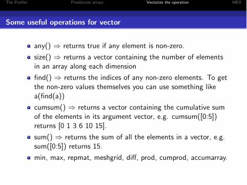
Some useful operations for vector
any() ) returns true if any element is non-zero.
size() ) returns a vector containing the number of elementsin an array along each dimension
find() ) returns the indices of any non-zero elements. To getthe non-zero values themselves you can use something likea(find(a))
cumsum() ) returns a vector containing the cumulative sumof the elements in its argument vector, e.g. cumsum([0:5])returns [0 1 3 6 10 15].
sum() ) returns the sum of all the elements in a vector, e.g.sum([0:5]) returns 15.
min, max, repmat, meshgrid, di↵, prod, cumprod, accumarray.

The Profiler Preallocate arrays Vectorize the operation MEX
Vectorized Logic
>> [1,5,3] < [2,2,4]ans = 1 0 1>> find([1,5,3] < [2,2,4]) % Find indices of nonzero elementsans = 1 3>> any([1,5,3] < [2,2,4])% True if any element of a vector isnonzero (or per-column for a matrix)ans = 1>> all([1,5,3] < [2,2,4]) %True if all elements of a vector arenonzero (or per-column for a matrix)ans = 0
Vectorized logic also works on arrays.>> find(eye(3) == 1) % Find which elements == 1 in the 3x3identity matrixans = 1 5 9 % (element locations given as indices)

Functions
MATLAB functions are similar to C functions.
MATLAB programs are stored as plain text in m-files. Each m-filecontains exactly one MATLAB function. Thus, a collection ofMATLAB functions can lead to a large number of relatively small files.
function [y1,...,yN] = myfun(x1,...,xM)
Exercise: Return the sum and di↵erence of two variables
Xin Zhang (STAT 598) Lecture 11 March 26th,2013 7 / 30

The Profiler Preallocate arrays Vectorize the operation MEX
Inlining Simple Functions
Every time an M-file function is called, the Matlab interpreterincurs some overhead. Additionally, many M-file functions beginwith conditional code that checks the input arguments for errors ordetermines the mode of operation.Example:y = zeros(size(x)); % Preallocatefor k = 3:length(x)-2
y(k) = median(x(k-2:k+2));end
Inlining a function means to replace a call to the function with thefunction code itself. The median function can be inclined.
tmp = sort(x(k-2:k+2));y(k) = tmp(3);
Matlab Programing Example
ReferenceAn Algorithmic Introduction to the Numerical Simulation of StochasticDi↵erential Equations
AuthorDesmond J. Higham
Xin Zhang (STAT 598) Lecture 11 March 26th,2013 8 / 30

Simulation of Brownian motion
W(0)=0 with Probability 1
W
j
= W
j�1 + dW
j
, j = 1, 2, . . . ,N (2)
Each dWj is an independent random variable of the formp�tN(0, 1)]
random number generator randn – each call to randu produces an”pseudorandom” number
Notice: Matlab starts arrays from index 1 and not index 0.
Xin Zhang (STAT 598) Lecture 11 March 26th,2013 9 / 30

Simulation of Brownian motion
%BPATH1 Browniam path simulation
randn(’state’,100) % set the state of randnT=1; N=500; dt=T/N;dW=zeros(1,N); % preallocate arraysW=zeros(1,N); % for e�ciency
dW(1)=sqrt(dt)*randn; % first approximation outside the loopW(1)=dW(1); % since W(0)=0 is not allowedfor j=2:NdW(j)=sqrt(dt)*randn; % general incrementW(j)=W(j-1)+dW(j);
end
plot([0:dt:T],[0,W],’r-’); %plot W against txlabel(’t’,’FomtSize’,16)ylabel(’W(t),’FontSize’,16,’Rotation’,0)
Xin Zhang (STAT 598) Lecture 11 March 26th,2013 10 / 30

Simulation of Brownian motion:vectorized
Instead of loop, we can perform the same computation more elegantlyand e�ciently using higher level ”vectorized” commands.
Function randn(i,N) creates a 1-by-N array of independent N(0,1)samples.
Function cumsum() computes the cummulative sum of its argument.
Xin Zhang (STAT 598) Lecture 11 March 26th,2013 11 / 30

Simulation of Brownian motion:vectorized
%BPATH2 Brownian path simulation: vectorized
randn(’state’,100) % set the state of randnT = 1; N = 500; dt = T/N;
dW = sqrt(dt)*randn(1,N); % incrementsW = cumsum(dW); % cumulative sum
plot([0:dt:T],[0,W],’r-’) % plot W against txlabel(’t’,’FontSize’,16)ylabel(’W(t)’,’FontSize’,16,’Rotation’,0)
Xin Zhang (STAT 598) Lecture 11 March 26th,2013 12 / 30

Approximation of Stochastic integrals
Given a suitable function h, consider two sums
Ito integralN�1X
i=0
h(tj
)(W (tj+1)�W (t
j
)) (3)
Stratonovich integral
N�1X
i=0
h(t
j
+ t
j+1
2)(W (t
j+1)�W (tj
)) (4)
Xin Zhang (STAT 598) Lecture 11 March 26th,2013 13 / 30

Example when h = W
%STINT Approximate stochastic integrals%% Ito and Stratonovich integrals of WdW
randn(state,100) % set the state of randnT = 1; N = 5 0; dt = T/N;
dW = sqrt(dt)*randn(1,N); % incrementsW = cumsum(dW); % cumulative sum
ito = sum([0,W (1 : end � 1)]. ⇤ dW )strat = sum((0.5 ⇤ ([0,W (1 :end � 1)] +W ) + 0.5 ⇤ sqrt(dt) ⇤ randn(1,N)). ⇤ dW )
itoerr = abs(ito � 0.5 ⇤ (W (end)^2� T ))straterr = abs(strat � 0.5 ⇤W (end)^2)
Xin Zhang (STAT 598) Lecture 11 March 26th,2013 14 / 30

Euler-Maruyama Method
A SDE is given by
Integral form
X (t) = X0 +
Zt
0f (X (s))ds +
Zt
0g(X (s))dW (s), 0 t T . (5)
Or di↵erential equation form
dX (t) = f (X (t))dt + g(X (t))dW (t), X (0) = X0, 0 t T .(6)
The Euler-Maruyama(EM) method takes the form
X
j
= X
j�1+f (Xj�1)�t+g(X
j�1)(W (⌧j
)�W (⌧j�1)), j = 1, 2, . . . , L.
(7)
Xin Zhang (STAT 598) Lecture 11 March 26th,2013 15 / 30
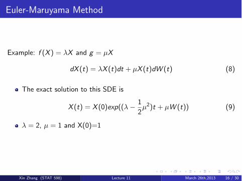
Euler-Maruyama Method
Example: f (X ) = �X and g = µX
dX (t) = �X (t)dt + µX (t)dW (t) (8)
The exact solution to this SDE is
X (t) = X (0)exp((�� 1
2µ2)t + µW (t)) (9)
� = 2, µ = 1 and X(0)=1
Xin Zhang (STAT 598) Lecture 11 March 26th,2013 16 / 30

Euler-Maruyama Method
%EM Euler-Maruyama method on linear SDE%% SDE is dX = lambda ⇤ Xdt +mu ⇤ XdW , X(0) = Xzero,% where lambda = 2, mu = 1 and Xzero = 1.%% Discretized Brownian path over [0,1] has dt = 2^ � 8.% Euler-Maruyama uses timestep R ⇤ dt.
randn(state,100)lambda = 2; mu = 1; Xzero = 1; % problem parametersT = 1;N = 2^8; dt = 1/N;dW = sqrt(dt) ⇤ randn(1,N); % Brownian incrementsW = cumsum(dW); % discretized Brownian pathXtrue = Xzero ⇤ exp((lambda� 0.5 ⇤mu
^2) ⇤ ([dt : dt : T ]) +mu ⇤W );plot([0:dt:T],[Xzero,Xtrue],’m-’), hold on
Xin Zhang (STAT 598) Lecture 11 March 26th,2013 17 / 30
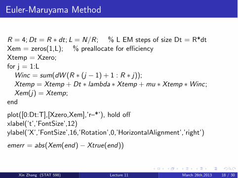
Euler-Maruyama Method
R = 4;Dt = R ⇤ dt; L = N/R ; % L EM steps of size Dt = R*dtXem = zeros(1,L); % preallocate for e�ciencyXtemp = Xzero;for j = 1:LWinc = sum(dW (R ⇤ (j � 1) + 1 : R ⇤ j));Xtemp = Xtemp + Dt ⇤ lambda ⇤ Xtemp +mu ⇤ Xtemp ⇤Winc ;Xem(j) = Xtemp;
end
plot([0:Dt:T],[Xzero,Xem],’r–*’), hold o↵xlabel(’t’,’FontSize’,12)ylabel(’X’,’FontSize’,16,’Rotation’,0,’HorizontalAlignment’,’right’)
emerr = abs(Xem(end)� Xtrue(end))
Xin Zhang (STAT 598) Lecture 11 March 26th,2013 18 / 30

Strong Convergence of the EM Method
A method is said to have strong order of convergence equal to � if thereexists a constant C such that
E |Xn
� X (⌧)| C�t
� (10)
for any fixed ⌧ = n�t 2 [0,T ] and �t e�ciently small.
We lete
Strong
�t
:= E |XL
� X (T )|, L�t = T (11)
The inequality (10) is equivalent to
e
Strong
�t
C�t
� (12)
for su�ciently small �t.
Xin Zhang (STAT 598) Lecture 11 March 26th,2013 19 / 30

Strong Convergence of the EM Method
Let’s look at the Strong convergence of EM for the SDE in our lastexample em.m with order � = 1/2.
Step 1: Compute 1000 di↵erent discretized Brownian paths over [0,1]with �t = 2�9.
Step 2: For each path, EM is applied with 5 di↵erent stepsize:�t = 2p�1�t for 1 p 5.
Step 3: Compute the endpoint error in the sth sample path for thepth stepsize and store it in Xerr(s,p)
Step 4: mean(Xeer(s,p)) will give us the approximation to e
Strong
�t
for5 di↵erent stepsize.
Xin Zhang (STAT 598) Lecture 11 March 26th,2013 20 / 30

Strong Convergence of the EM Method
If the inequality holds with approximation equality, then, taking logs, wehave
log eStrong�t
⇡ logC + 1/2 log�t (13)
Xin Zhang (STAT 598) Lecture 11 March 26th,2013 21 / 30

Strong Convergence of the EM Method
%EMSTRONG Test strong convergence of Euler-Maruyama%% Solves dX = lambda ⇤ Xdt +mu ⇤ XdW , X(0) = Xzero,% where lambda = 2, mu = 1 and Xzer0 = 1.%% Discretized Brownian path over [0,1] has dt = 2^ � 9.% E-M uses 5di↵erent timesteps: 16dt, 8dt, 4dt, 2dt, dt.% Examine strong convergence at T = 1 : E |X
L
� X (T )|.
randn(state,100)lambda = 2; mu = 1; Xzero = 1; % problem parametersT = 1; N = 2^9; dt = T/N;M = 1000; % number of paths sampled
Xin Zhang (STAT 598) Lecture 11 March 26th,2013 22 / 30

Strong Convergence of the EM Method
Xerr = zeros(M,5); % preallocate arrayfor s = 1:M, % sample over discrete Brownian pathsdW = sqrt(dt) ⇤ randn(1,N); % Brownian incrementsW = cumsum(dW); % discrete Brownian pathXtrue = Xzero ⇤ exp((lambda� 0.5 ⇤mu
^2) +mu ⇤W (end));for p = 1:5R = 2(p � 1);Dt = R ⇤ dt; L = N/R ;Xtemp = Xzero;for j = 1:LWinc = sum(dW (R ⇤ (j � 1) + 1 : R ⇤ j));Xtemp = Xtemp + Dt ⇤ lambda ⇤ Xtemp +mu ⇤ Xtemp ⇤Winc ;
endXerr(s, p) = abs(Xtemp � Xtrue); % store the error at t = 1
endend
Xin Zhang (STAT 598) Lecture 11 March 26th,2013 23 / 30

Strong Convergence of the EM Method
Dtvals = dt ⇤ (2.^([0 : 4]));loglog(Dtvals,mean(Xerr),0 b ⇤ �0); hold onloglog(Dtvals, (Dtvals.^(.5)),0 r ��0); hold o↵ % reference slope of 1/2axis([1e-3 1e-1 1e-4 1])xlabel(’\Delta t’);ylabel(’Sample average of|X (T )� X
L
|’)title(emstrong.m,FontSize,10)
%%%% Least squares fit of error = C ⇤ Dtq %%%%A = [ones(5, 1), log(Dtvals)]; rhs = log(mean(Xerr));sol = A \rhs; q = sol(2)resid = norm(A ⇤ sol � rhs)
Xin Zhang (STAT 598) Lecture 11 March 26th,2013 24 / 30

Weak Convergence of the EM Method
A method is said to have weak order of convergence equal to � if thereexists a constant C such that for all functions p in some class
|Ep(Xn
)� Ep(X (⌧))| C�t
� (14)
for any fixed ⌧ = n�t 2 [0,T ] and �t e�ciently small. We focus on thecase where p is identity function
We lete
Weak
�t
:= |EXL
� EX (T )|, L�t = T (15)
The inequality (14) is equivalent to
e
Weak
�t
C�t
� (16)
for su�ciently small �t.
Xin Zhang (STAT 598) Lecture 11 March 26th,2013 25 / 30

Weak Convergence of the EM Method
Let’s look at the Weak convergence of EM for the SDE in our lastexample em.m with order � = 1.
Step 1: Compute 1000 di↵erent discretized Brownian paths over [0,1]with �t = 2�9.
Step 2: For each path, EM is applied with 5 di↵erent stepsize:�t = 2p�1�t for 1 p 5.
Step 3: Compute the endpoint error in the sth sample path for thepth stepsize and store it in Xerr(s,p)
Step 4: mean(Xeer(s,p)) will give us the approximation to e
Strong
�t
for5 di↵erent stepsize.
Xin Zhang (STAT 598) Lecture 11 March 26th,2013 26 / 30

Weak Convergence of the EM Method
If the inequality holds with approximation equality, then, taking logs, wehave
log eStrong�t
⇡ logC + log�t (17)
Xin Zhang (STAT 598) Lecture 11 March 26th,2013 27 / 30

Weak Convergence of the EM Method
%EMWEAK Test weak convergence of Euler-Maruyama%% Solves dX = lambda ⇤ Xdt +mu ⇤ XdW , X(0) = Xzero,% where lambda = 2, mu = 1 and Xzer0 = 1.%% E-M uses 5di↵erent timesteps: 2^(p � 10), p = 1,2,3,4,5.% Examine weak convergence at T = 1 : |E (X
L
)� E (X (T ))|.%% Di↵erent paths are used for each E-M timestep.% Code is vectorized over paths.%% Uncommenting the line indicated below gives the weak E-M method.
randn(state,100);lambda = 2; mu = 0.1; Xzero = 1; T = 1; % problem parametersM = 50000;
Xin Zhang (STAT 598) Lecture 11 March 26th,2013 28 / 30

Weak Convergence of the EM Method
Xem = zeros(5,1); % preallocate arraysfor p =1:5 % take various Euler timestepsDt = 2^(p � 10); L = T/Dt; % L Euler steps of size DtXtemp = Xzero*ones(M,1);for j = 1:LWinc = sqrt(Dt)*randn(M,1)Xtemp = Xtemp + Dt ⇤ lambda ⇤ Xtemp +mu ⇤ Xtemp. ⇤Winc ;
endXem(p) = mean(Xtemp);
endXerr =abs(Xem � exp(lambda));
Xin Zhang (STAT 598) Lecture 11 March 26th,2013 29 / 30

Weak Convergence of the EM Method
Dtvals = 2.^([1 : 5]� 10);loglog(Dtvals,Xerr ,0 b ⇤ �0), hold onloglog(Dtvals,Dtvals,0 r ��0), hold o↵ % reference slope of 1axis([1e-3 1e-1 1e-4 1])xlabel(’\Delta t’), ylabel(’|E (X (T ))� Sample average of X
L
|’)title(’emweak.m’,’FontSize’,10)
%%%% Least squares fit of error = C ⇤ dtq %%%%A = [ones(p, 1), log(Dtvals)]; rhs = log(Xerr);sol = A\ rhs; q = sol(2)resid = norm(A*sol - rhs)
Xin Zhang (STAT 598) Lecture 11 March 26th,2013 30 / 30