matlab intro notes

Computational Finance using MATLAB

Brad BaxterDepartment of Economics, Mathematics and Statistics,

Birkbeck College, University of London,

Malet Street, London WC1E 7HX

[email protected]

This is a short introduction to scientific computation in MATLAB. It isdesigned for self-study by both GDFE and MSc students. 1

1. Introduction

These notes can be obtained from

http://econ109.econ.bbk.ac.uk/brad/CTFE/

and you can download lots of relevant material for MSc Financial Engineeringfrom

http://econ109.econ.bbk.ac.uk/brad/Methods/

This folder contains the current versions of methods notes.pdf and nabook.pdf.The book Numerical Methods in Finance and Economics: A MATLAB-

based Introduction, by P. Brandimarte, contains many excellent examples,and is strongly recommended for both CTFE and MSc Financial Engineering.I also recommend the undergraduate-level textbook An Introduction to FinancialOption Valuation, by D. Higham, which is particularly suitable for CTFE.

All of the programs in this note also work with Octave, which is a freequasi-clone of MATLAB, and can be found here:

http://www.gnu.org/software/octave/

Another good quasi-clone is

http://freemat.sourceforge.net/

You’re welcome to use the Computer Room; the door code is 5858.

1 Version: 201310241641

2 Brad Baxter

2. MATLAB Basics

2.1. Matrices and Vectors

MATLAB (i.e. MATrix LABoratory) was designed for numerical linearalgebra.

Notation: a p× q matrix has p rows and q columns; its entries are usuallyreal numbers in these notes, but they can also be complex numbers. A p×1matrix is also called a column vector, and a 1 × q matrix is called a rowvector. If p = q = 1, then it’s called a scalar.

We can easily enter matrices:

A = [1 2 3; 4 5 6; 7 8 9; 10 11 12]

In this example, the semi-colon tells Matlab the row is complete.The transpose AT of a matrix A is formed by swapping the rows and

columns:

A = [1 2 3; 4 5 6; 7 8 9; 10 11 12]

AT = A’

Sometimes we don’t want to see intermediate results. If we add a semi-colon to the end of the line, the MATLAB computes silently:

A = [1 2 3; 4 5 6; 7 8 9; 10 11 12];

AT = A’

Matrix multiplication is also easy. In this example, we compute AAT andATA.

A = [1 2 3; 4 5 6; 7 8 9; 10 11 12]

AT = A’

M1 = A*AT

M2 = AT*A

In general, matrix multiplication is non-commutative, as seen in Example2.1.

Example 2.1. As another example, let’s take two column vectors u andv in R4 and compute the matrix products u′v and uv′. The result mightsurprise you at first glance.

u = [1; 2; 3; 4]

v = [5; 6; 7; 8]

u’*v

u*v’

Exercise 2.1. What’s the general formula for uv′?

Computational Finance using MATLAB 3

2.2. The sum function

It’s often very useful to be able to sum all of the elements in a vector, whichis very easy in Matlab:

u = [1 2 3 4]

sum(u)

The sum is also useful when dealing with matrices:

A = [1 2; 3 4]

sum(A)

You will see that Matlab has summed each column of the matrix.

2.3. Solving Linear Equations

MATLAB can also solve linear equations painlessly:

n = 10

% M is a random n x n matrix

M = randn(n);

% y is a random n x 1 matrix, or column vector.

y = randn(n,1);

% solve M x = y

x = M\y

% check the solution

y - M*x

We shall need to measure the length, or norm, of a vector, and this isdefined by

‖v‖ =√v21 + v22 + · · ·+ v2n,

where v1, . . . , vn ∈ R are the components of the vector v; the correspondingMATLAB function is norm(v). For example, to check the accuracy of thenumerical solution of Mx = y, we type norm(y - M*x).

It’s rarely necessary to compute the inverse M−1 of a matrix, because it’susually better to solve the corresponding linear system Mx = y using

x = M\y

as we did above. However, the corresponding MATLAB function is inv(M).

2.4. The MATLAB Colon Notation

MATLAB has a very useful Colon notation for generating lists of equally-spaced numbers:

1:5

4 Brad Baxter

will generate the integers 1, 2, . . . , 5, while

1:0.5:4

will generate 1, 1.5, 2, 2.5, . . . , 3.5, 4, i.e. the middle number is the step-size.

Example 2.2. This example illustrates a negative step-length and theiruse to generate a vector.

v = [10:-1:1]’;

w = 2*v

We can easily extract parts of a matrix using the MATLAB colon notation.

A = [1 2 3; 4 5 6; 7 8 9; 10 11 12]

M = A(2:3, 2:3)

The following example illustrates the Matlab dot notation

Example 2.3. Consider the following MATLAB code.

A = [1 2; 3 4]

A^2

A.^2

The first command uses matrix multiplication to multiply A by itself, whilstthe second creates a new matrix by squaring every component of A.

Exercise 2.2. What does the following do?

sum([1:100].^2)

2.5. Graphics

Let’s learn more about graphics.

Example 2.4. Plotting a sine curve:

t = 0: pi/200: 2*pi;

y = sin(3*t);

plot(t,y)

Exercise 2.3. Replace plot(t,y) by plot(t,y,’o’) in the last example.

Example 2.5. See if you can predict the result of this code before typingit:

t = 0: pi/200: 2*pi;

y = sin(3*t).^2;

plot(t,y)

Exercise 2.4. Use the plot function to plot the graph of the quadraticp(x) = 2x2 − 5x+ 2, for −3 ≤ x ≤ 3.


Exercise 2.5. Use the plot function to plot the graph of the cubic q(x) =x3 − 3x2 + 3x− 1, for −10 ≤ x ≤ 10.

Here’s a more substantial code fragment producing a cardioid as theenvelope of certain circles. You’ll also see this curve formed by light reflectionon the surface of tea or coffee if there’s a point source nearby (halogen bulbsare good for this). It also introduces the axis command, which makes surethat circles are displayed as proper circles (otherwise MATLAB rescales,turning circles into ellipses).

Example 2.6. Generating a cardioid:

hold off

clf

t=0:pi/2000:2*pi;

plot(cos(t)+1,sin(t))

axis([-1 5 -3 3])

axis(’square’)

hold on

M=10;

for alpha=0:pi/M:2*pi

c=[cos(alpha)+1; sin(alpha)];

r = norm(c);

plot(c(1)+r*cos(t),c(2)+r*sin(t));

end

2.6. Getting help

You can type

help polar

to learn more about any particular command. Matlab has extensive documentationbuilt-in, and there’s lots of information available online.

3. Generating random numbers

Computers generate pseudorandom numbers, i.e. deterministic (entirelypredictable) sequences which mimic the statistical properties of randomnumbers. Speaking informally, however, I shall often refer to “randomnumbers” when, strictly speaking, “pseudorandom numbers” would be thecorrect term. At a deeper level, one might question whether anything is trulyrandom, but these (unsolved) philosophical problems need not concern atthis stage.

We shall first introduce the extremely important rand and randn functions.

6 Brad Baxter

Despite their almost identical names, they are very different, as we shallsee, and should not be confused. The rand function generates uniformlydistributed numbers on the interval [0, 1], whilst the randn function generatesnormally distributed, or Gaussian random numbers. In financial applications,randn is extremely important.

Our first code generating random numbers can be typed in as a program,using the create script facility, or just entered in the command window.

Example 3.1. Generating uniformly distributed random numbers:

N = 10000;

v=rand(N,1);

plot(v,’o’)

The function we have used here is rand(m,n), which produces an m× nmatrix of pseudorandom numbers, uniformly distributed in the interval [0, 1].

Using the plot command in these examples in not very satisfactory,beyond convincing us that rand and randn both produce distributions ofpoints which look fairly random. For that reason, it’s much better to use ahistogram, which is introduced in the following example.

Example 3.2. Uniformly distributed random numbers and histograms:

N = 10000;

v=rand(N,1);

nbins = 20;

hist(v,nbins);

Here Matlab has divided the interval [0, 1] into 20 equal subintervals, i.e.

[0, 0.05], [0.05, 0.1], [0.1, 0.15], . . . , [0.90, 0.95], [0.95, 1],

and has simply drawn a bar chart: the height of the bar for the interval[0, 0.05] is the number of elements of the vector v which lie in the interval[0.0.05], and similarly for the other sub-intervals.

Exercise 3.1. Now experiment with this code: change N and nbins.

Example 3.3. Gaussian random numbers and histograms:

N = 100000;

v=randn(N,1);

nbins = 50;

hist(v,nbins);

Observe the obvious difference between this bell-shaped distribution and thehistogram for the uniform distribution.

Exercise 3.2. Now experiment with this code: change N and nbins. Whathappens for large N and nbins?


As we have seen, MATLAB can easily construct histograms for Gaussian(i.e. normal) pseudorandom numbers. As N and nbins tend to infinity,the histogram converges to a curve, which is called the probability densityfunction (PDF). The formula for this curve is

p(s) = (2π)−1/2e−s2/2, for s ∈ R,

and the crucial property of the PDF is

P(a < Z < b) =

∫ b

ap(s) ds.

Example 3.4. Good graphics is often fiddly, and this example uses somemore advanced features of MATLAB graphics commands to display thehistogram converging nicely to the PDF for the Gaussian. I will not explainthese fiddly details in the lecture, but you will learn much from further studyusing the help facility. This example is more substantial so create a script,i.e. a MATLAB program – I will explain this during the lecture. Everyline beginning with % is a comment. i.e. it is only there for the humanreader, not the computer. You will find comments extremely useful in yourprograms.

% We generate a 1 x 5000 array of N(0,1) numbers

a = randn(1,5000);

% histogram from -3 to 3 using bins of size .2

[n,x] = hist(a, [-3:.2:3]);

% draw a normalized bar chart of this histogram

bar(x,n/(5000*.2));

% draw the next curve on the same plot

hold on

% draw the Gaussian probability density function

plot(x, exp(-x.^2/2)/sqrt(2*pi))

%

% Note the MATLAB syntax here: x.^2 generates a new array

% whose elements are the squares of the original array x.

hold off

Exercise 3.3. Now repeat this experiment several times to get a feel forhow the histogram matches the density for the standard normal distribution.Replace the magic numbers 5000 and 0.2 by N and Delta and see for yourselfhow much it helps or hinders to take more samples or smaller size bins.

3.1. The Central Limit Theorem

Where does the Gaussian distribution come from? Why does it occur inso many statistical applications? It turns out that averages of random

8 Brad Baxter

variables are often well approximated by Gaussian random variables, if therandom variables are not too wild, and this important theorem is calledthe Central Limit Theorem. The next example illustrates the Central LimitTheorem, and shows that averages of independent, uniformly distributedrandom variables converge to the Gaussian distribution.

Example 3.5. This program illustrates the Central Limit Theorem: suitablyscaled averages of uniformly distributed random variables look Gaussian, ornormally distributed. First we create a 20× 10000 matrix of pseudorandomnumbers uniformly distributed on the interval [0, 1], using the rand functions.We then sum every column of this matrix and divide by

√20.

m = 20;

n = 10000;

v = rand(m,n);

%

% We now sum each column of this matrix, divide by sqrt(m)

% and histogram the new sequence

%

nbins = 20

w = sum(v)/sqrt(m);

hist(w,nbins);

Exercise 3.4. Play with the constants m and n in the last example.

3.2. Gaussian Details

The Matlab randn command generates Gaussian pseudorandom numberswith mean zero and variance one; we write this N(0, 1), and such randomvariables are said to be normalized Gaussian, or standard normal. If Zis a normalized Gaussian random variable, then the standard notation toindicate this is Z ∼ N(0, 1), where “∼” means “is distributed as”. We caneasily demonstrate these properties in Matlab:

Example 3.6. Here we generate n normalized Gaussian pseudorandomnumbers Z1, . . . , Zn, and then calculate their sample mean

µ̂ =1

n

n∑k=1

Zk

and their sample variance

σ̂2 =1

n

n∑k=1

Z2k ,

as follows.


n=10000;

Z=randn(n,1);

mean(Z)

mean(Z.^2)

Experiment with this code, increasing n to 106, say.

Obviously not all random variables have mean zero and unit variance, butit’s simple to generate Gaussian random variables with any given mean µand variance σ2. Specifically, if Z ∼ N(0, 1), then W = µ+ σZ ∼ N(µ, σ2).It’s easy to illustrate this in Matlab.

Example 3.7. Here we generate n normalized Gaussian pseudorandomnumbers Z1, . . . , Zn, to represent a normalized Gaussian random variableZ ∼ N(0, 1). We then define W = µ+ σZ, and generate the correspondingpseudorandom W1, . . . ,Wn, finding their sample mean and variance

µ̂ =1

n

n∑k=1

Zk

and their sample variance

σ̂2 =1

n

n∑k=1

(Zk − µ̂)2 ,

as follows.

n=10000;

Z=randn(n,1);

mu = 1; sigma = 0.2;

W = mu + sigma*Z;

mu_hat = mean(W)

sigma_hat = sqrt(mean((W-mu_hat).^2))

Experiment with this code, increasing n to 106, say.

For reference, the PDF for a N(0, σ2) random variable is given by

p(s) = (2πσ2)−1/2e−s2/(2σ2), s ∈ R.

Exercise 3.5. What the PDF for a N(µ, σ2) random variable?

4. Some Finance

Now let’s discuss a financial application. We shall use Monte Carlo simulation.2

You can find a full mathematical treatment in my notes for Mathematical

2 This name originated with the brilliant mathematician John von Neumann, during hiswork on the Manhattan Project, the secret project building the first American atomicbombs during World War II. In the first Monte Carlo simulation, the sample paths

10 Brad Baxter

Methods, but we really only need the basics here. We shall assume that ourshare price S(t) is a random variable given by the following formula

S(t) = S(0)e(r−σ2/2)t+σ

√tZ , for t > 0,

where Z is a standard Gaussian random variable, S(0) = 42, r = 0.1 andσ = 0.2. These parameters were fairly typical for the NYSE in the 1990s,and this example was taken from Options, Futures and Other DerivativeSecurities, by J. C. Hull.

We cannot predict the future price S(T ) of our stock at time T , but we canapproximate the distribution of its possible values. In other words, we canpredict the likely behaviour of our asset in many possible futures, althoughits value in our future sadly remains a mystery.

Example 4.1. Predicting many possible futures at expiry time T :

S0 = 42;

r = 0.1;

T = 0.5;

sigma = 0.2;

N = 100000;

%

% generate asset prices at expiry

%

Z = randn(N,1);

ST = S0*exp( (r-(sigma^2)/2)*T + sigma*sqrt(T)*Z );

%

% display histogram of possible prices at expiry

%

nbins=40;

hist(ST,nbins);

Exercise 4.1. Try various values of N, sigma, T and nbins in the previousexample. What happens for, say, sigma=20?

Once we know how to generate likely future prices in this way, we canactually price a Euro put option: let us suppose we own the share already

were those of neutrons passing through Uranium, the aim being to estimate the massof the Uranium isotope U235 required for a successful fission bomb. The Americanteam used some of the first computers (more like programmable calculators, by ourstandards) to estimate some 64 kg of U235 would be sufficient, which was achievableusing the cumbersome technology required to separate the 0.07% of U235 from commonUranium ore; they were correct in their estimates. The German team, led by WernerHeisenberg, had neither computers nor simulation. Heisenberg estimated a 1000 kgof U235 would be required, and therefore gave up, ending the German atomic bombproject.


and wish to insure ourselves against a decrease in its value over the next 6months. Specifically, we wish to buy the right, but not the obligation, tosell the share at the exercise price K = $40 at T = 0.5. Such a contractis called a European put option, with exercise price (or strike price) K andexpiry time T = 0.5. Obviously we want to compute the fair price of sucha contract. Now, if S(T ) ≥ K, then the option is worth nothing at expiry;there is no value in being able to sell a share for K if it’s actually worthmore! In contrast, if S(T ) < K, then we have made a profit of K − S(T ).If we take the view that the fair price at expiry should be the average valueof max{K − S(T ), 0}, then we can easily compute this using the vector ST

of possible expiry prices calculated in the previous example. Specifically, wecompute the average

tput = sum(max(K-ST,0.0)/N;

To complete the pricing of this option, we need to understand the timevalue of money: we shall assume that we can borrow and save at the risk-free rate r. Thus, to obtain 1 at a time t in the future, we need only invest$ exp(−rt) now. In other words, the discounted future expected price of theEuropean put option is given by

fput = exp(-r*T)*sum(max(K-ST,0.0)/N;

Finally, here is a summary of all of the above.

Example 4.2. Using Monte Carlo simulation to approximate the value ofthe European put option of Example 11.6 of Hull:

%

% These are the parameters chosen in Example 11.6 of

% OPTIONS, FUTURES AND OTHER DERIVATIVES,

% by John C. Hull (Prentice Hall, 4th edn, 2000)

%

%% initial stock price

S0 = 42;

% unit of time = year

% continuous compounding risk-free rate

%

r = 0.1;

% exercise price

K = 40;

% time to expiration in years

T = 0.5;

% volatility

sigma = 0.2;

% generate asset prices at expiry

12 Brad Baxter

N=10000;

Z = randn(N,1);

ST = S0*exp( (r-(sigma^2)/2)*T + sigma*sqrt(T)*Z );

% calculate put contract values at expiry

fput = max(K - ST,0.0);

% average put values at expiry and discount to present

mc_put = exp(-r*T)*sum(fput)/N

Exercise 4.2. Modify this example to calculate the Monte Carlo approximationfor a European call, for which the contract value at expiry is given by

max(ST - K, 0)

Exercise 4.3. Modify the code to calculate the Monte Carlo approximationto a digital call, for which the contract value at expiry is given by

(ST > K);

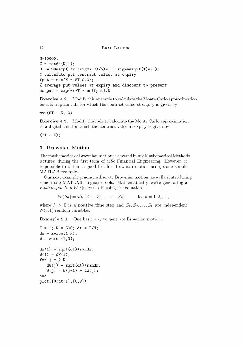
5. Brownian Motion

The mathematics of Brownian motion is covered in my Mathematical Methodslectures, during the first term of MSc Financial Engineering. However, itis possible to obtain a good feel for Brownian motion using some simpleMATLAB examples.

Our next example generates discrete Brownian motion, as well as introducingsome more MATLAB language tools. Mathematically, we’re generating arandom function W : [0,∞)→ R using the equation

W (kh) =√h (Z1 + Z2 + · · ·+ Zk) , for k = 1, 2, . . . ,

where h > 0 is a positive time step and Z1, Z2, . . . , Zk are independentN(0, 1) random variables.

Example 5.1. One basic way to generate Brownian motion:

T = 1; N = 500; dt = T/N;

dW = zeros(1,N);

W = zeros(1,N);

dW(1) = sqrt(dt)*randn;

W(1) = dW(1);

for j = 2:N

dW(j) = sqrt(dt)*randn;

W(j) = W(j-1) + dW(j);

end

plot([0:dt:T],[0,W])


The MATLAB function cumsum calculates the cumulative sum performedby the for loop in the last program, which makes life much easier.

Example 5.2. A more concise way to generate Brownian motion:

T = 1; N = 10000; dt = T/N;

dW = sqrt(dt)*randn(1,N); plot([0:dt:T],[0,cumsum(dW)])

Now play with this code, changing T and N.

Example 5.3. We can also use cumsum to generate many Brownian samplepaths:

T = 1; N = 500; dt = T/N;

nsamples = 10;

hold on

for k=1:nsamples

dW = sqrt(dt)*randn(1,N); plot([0:dt:T],[0,cumsum(dW)])

end

Exercise 5.1. Increase nsamples in the last example. What do you see?

5.1. Geometric Brownian Motion (GBM)

The idea that it can be useful to model asset prices using random functionswas both surprising and implausible when Louis Bachelier first suggestedBrownian motion in his thesis in 1900. There is an excellent translation ofhis pioneering work in Louis Bachelier’s Theory of Speculation: The Originsof Modern Finance, by M. Davis and A. Etheridge. However, as you havealready seen, a Brownian motion can be both positive and negative, whilst ashare price can only be positive, so Brownian motion isn’t quite suitable as amathematical model for share prices. Its modern replacement is to take theexponential, and the result is called Geometric Brownian Motion (GBM).In other words, the most common mathematical model in modern finance isgiven by

S(t) = S(0)eµt+σW (t), for t > 0,

where µ ∈ R is called the drift and σ is called the volatility.

Example 5.4. Generating GBM:

T = 1; N = 500; dt = T/N;

t = 0:dt:T;

dW = sqrt(dt)*randn(1,N);

mu = 0.1; sigma = 0.01;

plot(t,exp(mu*t + sigma*[0,cumsum(dW)]))

14 Brad Baxter

Exercise 5.2. Now experiment by increasing and decreasing the volatilitysigma.

In mathematical finance, we cannot predict the future, but we estimategeneral future behaviour, albeit approximately. For this we need to generateseveral Brownian motion sample paths, i.e. several possible futures for ourshare. The key command will be randn(M,N), which generates an M × Nmatrix of independent Gaussian random numbers, all of which are N(0, 1).We now need to tell the cumsum function to cumulatively sum along eachrow, and this is slightly more tricky.

Example 5.5. Generating several GBM sample paths:

T = 1; N = 500; dt = T/N;

t = 0:dt:T;

M=10;

dW = sqrt(dt)*randn(M,N);

mu = 0.1; sigma = 0.01;

S = exp(mu*ones(M,1)*t + sigma*[zeros(M,1), cumsum(dW,2)]);

plot(t,S)

Here the MATLAB function ones(p,q) creates a p × q matrix of ones,whilst zeros(p,q) creates a p × q matrix of zeros. The matrix productones(M,1)*t is a simple way to create an M ×N matrix whose every rowis a copy of t.

Exercise 5.3. Experiment with various values of the drift and volatility.

Exercise 5.4. Copy the use of the cumsum function in Example 5.5 toavoid the for loop in Example 5.3.


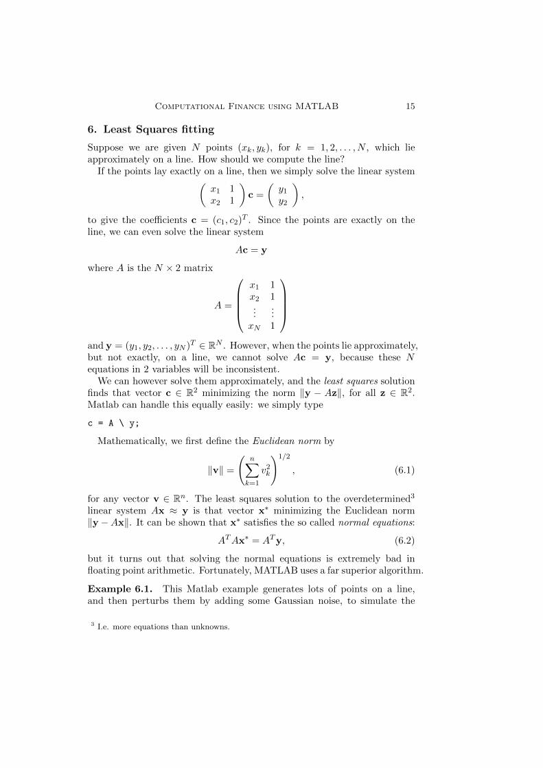
6. Least Squares fitting

Suppose we are given N points (xk, yk), for k = 1, 2, . . . , N , which lieapproximately on a line. How should we compute the line?

If the points lay exactly on a line, then we simply solve the linear system(x1 1x2 1

)c =

(y1y2

),

to give the coefficients c = (c1, c2)T . Since the points are exactly on the

line, we can even solve the linear system

Ac = y

where A is the N × 2 matrix

A =

x1 1x2 1...

...xN 1

and y = (y1, y2, . . . , yN )T ∈ RN . However, when the points lie approximately,but not exactly, on a line, we cannot solve Ac = y, because these Nequations in 2 variables will be inconsistent.

We can however solve them approximately, and the least squares solutionfinds that vector c ∈ R2 minimizing the norm ‖y − Az‖, for all z ∈ R2.Matlab can handle this equally easily: we simply type

c = A \ y;

Mathematically, we first define the Euclidean norm by

‖v‖ =

(n∑k=1

v2k

)1/2

, (6.1)

for any vector v ∈ Rn. The least squares solution to the overdetermined3

linear system Ax ≈ y is that vector x∗ minimizing the Euclidean norm‖y−Ax‖. It can be shown that x∗ satisfies the so called normal equations:

ATAx∗ = ATy, (6.2)

but it turns out that solving the normal equations is extremely bad infloating point arithmetic. Fortunately, MATLAB uses a far superior algorithm.

Example 6.1. This Matlab example generates lots of points on a line,and then perturbs them by adding some Gaussian noise, to simulate the

3 I.e. more equations than unknowns.

16 Brad Baxter

imperfections of real data. It then computes the least squares line of bestfit.

%

% We first generate some

% points on a line and add some noise

%

a0=1; b0=0;

n=100; sigma=0.1;

x=randn(n,1);

y=a0*x + b0 + sigma*randn(n,1);

%

% Here’s the least squares linear fit

% to our simulated noisy data

%

A=[x ones(n,1)];

c = A\y;

%

% Now we plot the points and the fitted line.

%

plot(x,y,’o’);

hold on

xx = -2.5:.01:2.5;

yy=a0*xx+b0;

zz=c(1)*xx+c(2);

plot(xx,yy,’r’)

plot(xx,zz,’b’)

Exercise 6.1. What happens when we increase the parameter sigma?

Exercise 6.2. Least Squares fitting is an extremely useful technique, butit is extremely sensitive to outliers. Here is a MATLAB code fragment toillustrate this:

%

% Now let’s massively perturb one data value.

%

y(n/2)=100;

cnew=A\y;

%

% Exercise: display the new fitted line. What happens when we vary the

% value and location of the outlier?

%


7. General Least Squares

There is no reason to restrict ourselves to linear fits. If we wanted to fita quadratic p(x) = p0 + p1x + p2x

2 to the data (x1, y1), . . . , (xN , yN ), thenwe can still compute the least squares solution to the overdetermined linearsystem

Ap ≈ y,

where p = (p0, p1, p2)T ∈ R3 and A is now the N × 3 matrix given by

A =

x21 x1 1x22 x2 1...

......

x2N xN 1

.

This requires a minor modification to Example 6.1.

Example 7.1. Generalizing Example 6.1, we generate a quadratic, perturbthe quadratic by adding some Gaussian noise, and then fit a quadratic tothe noisy data.

%


% points using the quadratic x^2 - 2x + 1 and add some noise

%

a0=1; b0=-2; c0=1;

n=100; sigma=0.1;

x=randn(n,1);

y=a0*(x.^2) + b0*x + c0 + sigma*randn(n,1);

%

% Here’s the least squares quadratic fit


%

A=[x.^2 x ones(n,1)];

c = A\y;

%

% Now we plot the points and the fitted quadratic

%

plot(x,y,’o’);

hold on

xx = -2.5:.01:2.5;

yy=a0*(xx.^2)+b0*xx + c0;

zz=c(1)*(xx.^2)+c(2)*xx + c(3);

plot(xx,yy,’r’)

plot(xx,zz,’b’)

18 Brad Baxter

Exercise 7.1. Increase sigma in the previous example, as for Example 6.1.Further, explore the effect of choosing a large negative outlier by adding theline y(n/2)=-10000; before solving for c.

There is absolutely no need to restrict ourselves to polynomials. Supposewe believe that our data (x1, y1), . . . , (xN , yN ) are best modelled by a functionof the form

s(x) = c0 exp(−x) + c1 exp(−2x) + c2 exp(−3x).

We now compute the least squares solution to the overdetermined linearsystem Ap ≈ y, where p = (p0, p1, p2)

T ∈ R3 and

A =

e−x1 e−2∗x1 e−3x1

e−x2 e−2∗x2 e−3x2

......

...e−xN e−2∗xN e−3xN

.

Example 7.2. %


% points using the function

% a0*exp(-x) + b0*exp(-2*x) + c0*exp(-3*x)

% and add some noise

%

a0=1; b0=-2; c0=1;

n=100; sigma=0.1;

x=randn(n,1);

y=a0*exp(-x) + b0*exp(-2*x) + c0*exp(-3*x) + sigma*randn(n,1);

%

% Here’s the least squares fit


%

A=[exp(-x) exp(-2*x) exp(-3*x)];

c = A\y;

%

% Now we plot the points and the fitted quadratic

%

plot(x,y,’o’);

hold on

xx = -2.5:.01:2.5;

yy=a0*exp(-xx)+b0*exp(-2*xx) + c0*exp(-3*xx);

zz=c(1)*exp(-xx)+c(2)*exp(-2*xx) + c(3)*exp(-3*xx);

plot(xx,yy,’r’)

plot(xx,zz,’b’)


8. Warning Examples

In the 1960s, mainframe computers became much more widely availablein universities and industry, and it rapidly became obvious that it wasnecessary to provide software libraries to solve common numerical problems,such as the least squares solution of linear systems. This was a golden age forthe new discipline of Numerical Analysis, straddling the boundaries of puremathematics, applied mathematics and computer science. Universities andnational research centres provided this software, and three of the pioneeringgroups were here in Britain: the National Physical Laboratory, in Teddington,the Atomic Energy Research Establishment, near Oxford, and the NumericalAlgorithms Group (NAG), in Oxford. In the late 1980s, all of this codewas incorporated into MATLAB. The great advantage of this is that thenumerical methods chosen by MATLAB are excellent and extremely welltested. However any method can be defeated by a sufficiently nasty problem,so you should not become complacent. The following matrix is usually calledthe Hilbert matrix, and seems quite harmless on first contact: it is the n×nmatrix H(n) whose elements are given by the simple formula

H(n)jk =

1

j + k + 1, 1 ≤ j, k ≤ n.

MATLAB knows about the Hilbert matrix: you can generate the 20 × 20Hilbert matrix using the command A = hilb(20);. The Hilbert matrix isnotoriously ill-conditioned, and the practical consequence of this property isshown here:

Example 8.1. %

% A is the n x n Hilbert matrix

%

n = 15;

A = hilb(n);

%

%

%

v = [1:n]’;

w = A * v;

%

% If we now solve w = A*vnew using vnew = A \ w,

% then we should find that vnew is the vector v.

% Unfortunately this is NOT so . . .

%

vnew = A \ w

Exercise 8.1. Try increasing n in the previous example.

20 Brad Baxter

8.1. Floating Point Warnings

Computers use floating point arithmetic. You shouldn’t worry about thistoo much, because the relative error in any arithmetic operation is roughly10−16, and we shall make this more precise below. However, it is not the sameas real arithmetic. In particular, errors can be greatly magnified and theorder of evaluation can affect results. For example, floating point additionis commutative, but not associative: a+ (b+ c) 6= (a+ b) + c, in general.

In this section, we want to see the full form of numbers, and not just thefirst few decimal places. To do this, use the MATLAB command format

long.

Example 8.2. Prove that

1− cosx

x2=

sin2 x

x2 (1 + cosx).

Let’s check this identity in MATLAB:

for k=1:8, x=10^(-k); x^(-2)*(1-cos(x)), end

for k=1:8, x=10^(-k); x^(-2)*sin(x)^2/(1+cos(x)), end

Explain these calculations. Which is closer to the truth?

We can also avoid using loops using MATLAB’s dot notation for pointwiseoperations. I have omitted colons in the next example to illustrate this:

x=10.^(-[1:8])

1-cos(x)

(sin(x).^2) ./ (1+cos(x))

Example 8.3. Prove that

√x+ 1−

√x =

1√x+ 1 +

√x,

for x > 0. Now explain what happens when we try these algebraically equalexpressions in MATLAB:

x=123456789012345;

a=sqrt(x+1)-sqrt(x)

a = 4.65661287307739e-08

b=1/(sqrt(x+1) + sqrt(x))

b = 4.50000002025000e-08

Which is correct?

Example 8.4. You should know from calculus that

exp(z) =∞∑k=0

zk

k!,


for any z ∈ C. Let’s test this.

x=2; S=1; N=20; for k=1:N, S=S+(x^k)/factorial(k); end

exp(x)

S

Now replace x=2 by x=-20. What has happened? What happens if weincrease N?

Example 8.5. The roots of the quadratic equation

x2 + bx+ c = 0

are given by

x1 =−b+

√b2 − 4c

2and x2 =

−b−√b2 − 4c

2.

Use these expressions to find the roots when b = 1111111; c=1. Now theidentity

x2 + bx+ c = (x− x1)(x− x2)

implies that c = x1x2. Is c/x2 equal to your computed value of x1? Whathas occurred?

8.2. Machine Precision

The smallest number ε such that the computer can distinguish 1 + ε from1 is called the machine epsilon. We can easily find this using the followingMatlab code:

Example 8.6. The following code generates a 55 × 4 matrix for whichrow k contains k, 2−k, 1 + 2−k, and finally a true/false value (i.e. 1 or 0)depending on whether MATLAB believes that 1 + 2−k exceeds 1.

x=zeros(55,0);

for k=1:55

x(k,1)=k; x(k,2)=2^(-k); x(k,3) = 1+x(k,2);

x(k,4) = (x(k,3) > 1); % equals 1 if x(k,3) > 1 else 0

end

You should find that ε = 2−52 = 16−13 = 2.22044604925031 × 10−16. Thiswill be the case on almost all computers, which now follow the IEEE 754standard specifying the details of floating point arithmetic, without whichour machines’ computations would be far more dubious.

Example 8.7. In the previous example, you should also observe that thethird column contains 1 for k ≥ 48. This is because you’re not seeing thebinary number itself, but its translation into base 10. The fact that the

22 Brad Baxter

computer’s arithmetic is binary, not decimal, can produce some initiallysurprising results. For example, the code fragment (10*0.1 < 10) willproduce the number 1, indicating that MATLAB believes the inequalityto be valid. Why isn’t 10 ∗ 0.1 exactly equal to 1?

Exercise 8.2. Construct values of a, b and c for which a + (b + c) 6=(a+ b) + c, implying that floating point arithmetic is not associative.


9. Recursion and Sudoku

This section is really just for fun, but it also gives me a chance to displaysome other features of the MATLAB language, of which the most importantis recursion: a MATLAB function can call itself.

Sudoku is a popular puzzle in which a 9× 9 matrix is further sub-dividedinto 9 3× 3 submatrices. The matrix can only contain the integers 1, . . . , 9,but each row, each column, and each of the 9 3 × 3 submatrices, mustcontain all 9 digits. Initially, the solver is faced with some given values, theremainder being blank. Here’s a simple example:

2 5 3 9 1

1 4

4 7 2 8

5 2

9 8 1

4 3

3 6 7 2

7 3

9 3 6 4

Here’s a harder example:

24 Brad Baxter

2 3 9 7

1

4 7 2 8

5 2 9

1 8 7

4 3

6 7 1

7

9 3 2 6 5It’s not too difficult to write a MATLAB program which can solve anySudoku. You can download a simple Sudoku solver (sud.m) from my officemachine:

http://econ109.econ.bbk.ac.uk/brad/CTFE/matlab_code/sudoku/

Here’s the MATLAB code for the solver:

function A = sud(A)

global cc

cc = cc+1;

% find all empty cells

[yy xx]=find(A==0);

if length(xx)==0

disp(’solution’)

disp(A);

return

end

x=xx(1);

y=yy(1);


for i=1:9 % try 1 to 9

% compute the 3 x 3 block containing this element

y1=1+3*floor((y-1)/3); % find 3x3 block

x1=1+3*floor((x-1)/3);

% check if i is in this element’s row, column or 3 x 3 block

if ~( any(A(y,: )==i) | any(A(:,x)==i) | any(any(A(y1:y1+2,x1:x1+2)==i)) )

Atemp=A;

Atemp(y,x)=i;

% recursively call this function

Atemp=sud(Atemp);

if all(all(Atemp))

A=Atemp; % ... the solution

return; % and that’s it

end

end

end

Download and save this file as sud.m. You can try the solver with thefollowing example:

%

% Here’s the initial Sudoku; zeros indicate blanks.

%

M0 = [

0 4 0 0 0 0 0 6 8

7 0 0 0 0 5 3 0 0

0 0 9 0 2 0 0 0 0

3 0 0 5 0 0 0 0 7

0 0 1 2 6 4 9 0 0

2 0 0 0 0 7 0 0 6

0 0 0 0 5 0 7 0 0

0 0 6 3 0 0 0 0 1

4 8 0 0 0 0 0 3 0];

M0

M = M0;

%

% cc counts the number of calls to sud, so it one measure

% of Sudoku difficulty.

%

global cc = 0;

sud(M);

cc

26 Brad Baxter

Exercise 9.1. Solve the first two Sudokus using sud.m.

Exercise 9.2. How does sud.m work?

matlab intro notes

Technology