mathematics regression analysis -lec-11.docx · let me talk about, the criteria for evaluating the...
TRANSCRIPT

Regression Analysis Prof. Soumen Maity
Department of Mathematics Indian Institute of Technology, Kharagpur
Lecture - 11
Selecting the BEST Regression Model (Contd.)
Hi, this is my second lecture on Selecting Best Regression Model, suppose you have a
problem with large number of regressors. And one response variable having large
number of regressors you may wonder, whether some them are irrelevant for the
response variable, and whether those irrelevant regressor variables can be removed from
the model, without affecting the model predictive power.
So, by the best regression model in multiple linear regression setup, we mean a model
that can explain the variability in y, and at the same time it includes as few regressors as
possible. Because, you know more regressors in a model, if you have more regessors in
the model then greater the cost of collecting the data, and also the cost for the
maintenance increases. Well, so the known algorithms for a selecting the best regression
model, they are basically classified into two classes, one is called a all possible
regression approach, and other one is the called a sequential selection.
So, in all possible regression approach what we did is that, if you have a problem with
you know k minus 1 regressors, then you consider all the 2 to the power of k minus 1
linear models. And the next step is that we fit those models, and we evaluate them with
respect to some criteria. So, the criteria could be the coefficient to multiple
determination, which is called you know r square, the criteria could be MS residual. It
could be adjusted coefficient of multiple determination that I am going to talk about this
one today, and also it could be the values statistics the is denoted by c p.

(Refer Slide Time: 04:20)
Let me talk about, the criteria for evaluating the subset tigation model one criteria is, a
residual mean square. So, we denoted by MS residual, so what we observed in the last
class is that SS residual P by this we mean that, the residual sum square for a model
involving P minus 1 regressors. So, this one decreases as the number of regressors
increases, but same is not necessarily true for MS residual, so MS residual may increase
if you increase a number of regressors, also that is what we observed in the last class.
Now, well what is the MS residual, MS residual is MS residual associated with a model
involving P minus 1 regressors is equal to SS residual P by n minus P and of courses,
you know lower value of MS residual P, indicates better fit. So, now, we will what we
will do is that, we will plot a MS residual, minimum MS residual against P, so P is the
number of unknown parameters in the model. And we will plot minimum MS residual
along the y axis right. So, what we do is that see given a P all possible models with P
minus 1 regressors are evaluated and a model giving minimum MS residual P is
tabulated. So, to explain this one let me recall my one example, we discussed in the last
class.

(Refer Slide Time: 08:48)
So, we will be considering the same example the HALD cement data, so here we have
four regressors, and one respond variable. So, here K is equal to K minus 1 is equal to 4
K minus 1 denotes the number of, so here K minus 1 is equal to 4. So, K minus 1 stands
for the number of regressors, well.
(Refer Slide Time: 09:24)
And then what we do is that we write down the models all possible models, so here this
is a model I said with no regressors. So, the number of regressors variable is equal to
equal to 0 here, equal to 0 here, so that is why P, P is the number of unknown, so there is

only one unknown that is the intercepted, so P is equal to 1 for this model. Now, these
are the model involving one regressor or we will say that these are called one regressor
model, that is why P equal to 2. Because, the number of unknowns for these models is
equal to 2, these are the model with involving two regressors that is why P equal to 3.
(Refer Slide Time: 10:22)
And these are the model involving three regressor, and P is equal to 4 and this is the full
model involving all the four regressor variables that is why P is equal to 5. And then first
we write down all possible models.
(Refer Slide Time: 10:55)

And then we take one model and we fit that model that is what we did in the last class,
you consider the model beta naught, beta 1, x 1 plus epsilon, and you compute the SS
total, SS residual, SS regression. And you write down the anova table, here is the anova
table for the first model and similarly, you have to do the same job for all possible, for all
the 16 possible models well. Now, what is the MS residual here, the MS residual for this
model is 115.1.
(Refer Slide Time: 11:48)
So, that is mentioned here the MS residual for this model is 115.06 more precisely, and
similarly you fit the second model you get the anova table you find out the MS residual
value. So, this way you compute the MS residual value for all the models, involving one
regressor for all the models involving two regressor variables, these are the MS residual.
And similarly, for the other models also you compute the MS residual value. Now, what
we do is that you know the minimum MS residual value in this class is 80.35. So, we
tabulate this one and the minimum in this class is 5.7, so we will take tabulate this one in
our this grapier.

(Refer Slide Time: 13:10)
So, for P equal to 1, P equal to 2, 3, 4, 5 well for P equal to 1; that means, there is no P
equal to 1 means this model no regressor, the MS residual value is 2, 2, 6 right. Suppose
this is 10, 20, 30 then it is you know may be 200 here. So, for P equal to 1 it is 2, 2, 6, so
somewhere here. Now, for P equal to 1 it is 2, 2, 6 for p equal to 2 it is 80.35, so you plot
somewhere here I am not very particular about this scaling, now for P equal to 3 it is 5.7.
So, somewhere here for P equal to 4, it is the minimum 1 is 5.33, so and for p equal to 5
it is 5.98, well this is 5.33 and 5.98.
So, what happen here is the this value is for MS residual 3 is equal to 5.7, MS residual 4
for P equal to 4 it is 5.33, and MS residual 5 for P equal to 5 it is 5.98. So, what happens
here is that initially you know, initially MS residual decreases and then it stabilizes for
some time and then it may increase also. So, here it is increasing little bit from 5.33 to
5.98, so this you know because for SS residual it is not true, SS residual is always
decreasing function.
But, that same is not true for the SS residual sorry the same is not true for MS residual.
So, it may increase also, so if the newly added regression variable is not relevant to the
response variable, then the reduction you know the reduction in SS regression is not
sufficient to compensate the 1 degree of freedom loss in the denominator that is why MS
residual increases also some for sometime well.

(Refer Slide Time: 17:35)
So, what we do here, so the we choose a value p, such that MS residual P is almost equal
to the MS residual for the full model or we choose a value of p, such that value of p
where MS residual P turns upward. So, here these are the I mean selection criteria either
you choose a p, in fact, it is a number of regressors in the regression model p minus 1.
So, you choose a P such that the MS residual P is almost close to the MS residual for the
full model, otherwise you choose a P such that from that point MS residual P turns
upward.
(Refer Slide Time: 19:20)

So, here you can see that you know MS residual decreases till P equal to 4, and then it
turns upward because for 5 it is again the value is more than the value for P equal to 4.
So, here it turns upward, so here you can choose P equal to 4 the meaning of this one is
that.
(Refer Slide Time: 19:52)
So, this MS residual criteria suggest that you go for the model involving the regressor x
1, x 2, x 4 also you know this other two models, like. The model involving x 1, x 2, x 3
and the model involving x 1, x 3, and x 4, they have also you know the comparable value
of MS residual, so either it can go for this model or the these two models. And if you
prefer you know, the model with two variables then of course, you have to go for the
model with which involves x 1 and x 2 of course, this is how we evaluate the a model
using the MS residual criteria. Now, next we are going to talk about one more criteria
that is called a adjusted coefficient of multiple determination.

(Refer Slide Time: 21:21)
And this one is denoted by R bar square well, so let me just a call R square, R square is
the coefficient of multiple determination, which is equal to SS regression by SS total.
And this one is equal to if I this 1 is equal to 1 minus SS residual by SS T, now if I say
this R square is associated with the model, which involves P minus 1 regressor, then I
will put P here, one P here, and one p here. Now, what we know is that SS residual P
always decreases as P increases.
So, from here you can say that this implies this statement implies that coefficient of
determination R square P this always increases as P increases. So, from here you know
we can say that R square P or R square is not a good measure of the quality of fit, let me
explain why because see whether the newly inserted or newly included regressor variable
is relevant to the model or not. Irrespective of that fact whatever regressor variable you
include, SS residual always decreases and R square always increases with the, when the
number of regressor variable is here, number of regressor variable increases.
So, that is why you know R square is R square cannot distinguish between whether the
newly added regressor variable is relevant for the model or it is irrelevant for the model.
So, that is why R square is or r square or SS residual is not a good measure, to check the
quality of fit well. So, that is why what we define is that we define, we introduce
adjusted coefficient of multiple determination, so what is that this R P bar square, this is
the adjusted coefficient of multiple determination. The only difference is that here you
know, we replace this SS residual P by MS residual P.
And here, we replace the SS T by MS T and then this can be written as, now this
adjusted you know R square can be written in terms of R square. So, this one is equal to
1 minus, what is MS residual when there are P minus 1 regressor in m model, I can write
that as SS residual by the degree of freedom n minus p. So, this is nothing, but MS
residual P right, now what is SS T, SS sorry MS T, MS T is nothing, but SS T by the
degree of freedom is n minus 1.
So, this one is equal to 1 minus n minus 1 by n minus p into SS residual P by SS T and
this 1 is nothing, but you know 1 minus R square. So, this can be written as 1 minus n
minus 1 by n minus p into 1 minus R P square, and since you know here we have
replaced SS residual by MS residual as I said before that MS residual will not necessarily
always decrease as P increases. So, here from there you can say that you know R P
square you can observe that R P bar square value will not necessarily increase with a
addition of any regressor. So, that is why this adjusted coefficient of multiple
determination, it is a better measure than the usual R square.
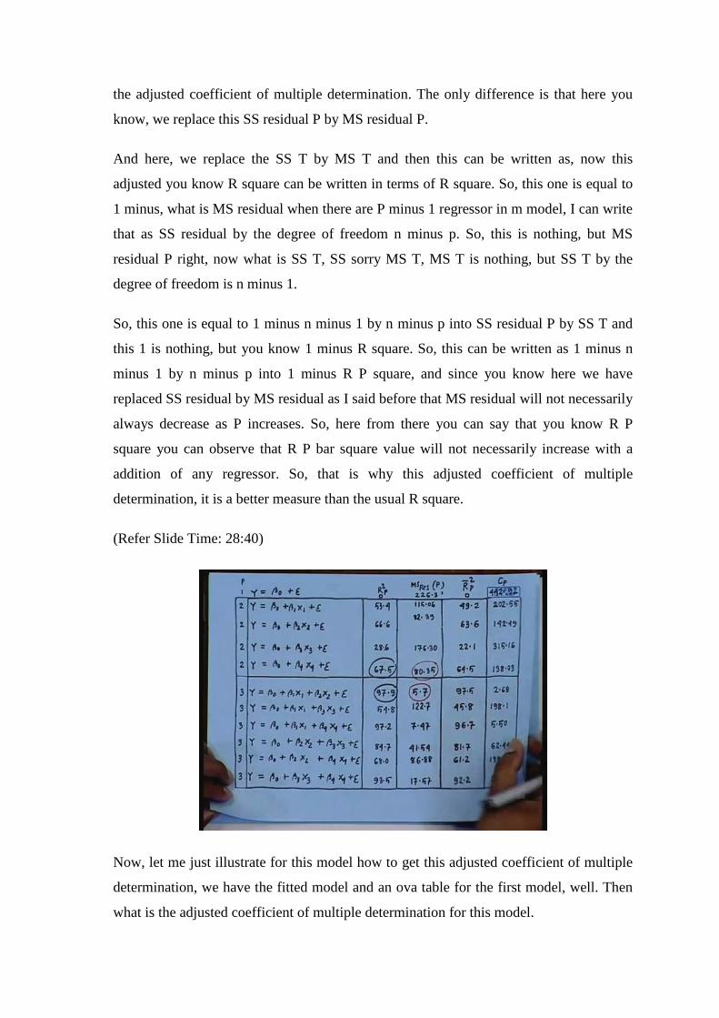
(Refer Slide Time: 28:40)
Now, let me just illustrate for this model how to get this adjusted coefficient of multiple
determination, we have the fitted model and an ova table for the first model, well. Then
what is the adjusted coefficient of multiple determination for this model.

(Refer Slide Time: 29:03)
So, there p equal to for this model Y equal to beta naught plus beta 1 x 1 plus epsilon.
So, here number of unknowns is equal to p, so p equal to 2. So, basically I computing R
2 bar square for this model, for this specific model. So, this 1 is equal to 1 minus n minus
that is 13 minus 1 12 by n minus p n is equal to 13 for that you know HALD cement
data. So, n minus p is equal to 11 and 1 minus R square R 2 square, so what is a value of
this R 2 square the value was 53.4 percent here.
So, basically this one is nothing, but 0.534. So, R 2 square is nothing, but SS regression
by SS total, which is equal to 1450 by 2715 please refer my previous class. So, this one
is equal to 0.534, so this value is equal to 1 minus 12 by 11 1 minus 0.534 which is going
to be equal to 0. 492. So, this way, so this value of the adjusted coefficient of multiple
determination for the first model is 0.49.

(Refer Slide Time: 31:15)
So, here is I am writing in percent, so it is a instead of 0.492 I am writing 49.2 percent.
So, similarly you fit the second model you get the, you will get the value of adjusted
coefficient of multiple determination similarly you do for all the model.
(Refer Slide Time: 31:40)
Here and for all the model involving three regressors, and four regressors these are the
value well. So, what we do is that we plot coefficient of adjusted coefficient of multiple
determination against the value of a P.

(Refer Slide Time: 32:20)
So, here also you all possible models with P minus 1 regressors are evaluated and model
giving maximum R P bar square is tabulated. So, of course, you know higher value of
adjusted coefficient of multiple determination, indicates a better fit that is why we
consider the maximum value, from each class R P bar square well. So, what we know is
that the maximum 1, 2, 3, 4, 5 and let me put 20, 40, 60, 80, 100, right let me have the
values. So, R P equal to 1 when P equal to 1 the value is equal to 0. When P equal to 2,
the maximum value is 64.5, when P equal to 3 the maximum value is 97.5.
(Refer Slide Time: 34:51)

When P equal to 4, the maximum value is 97.6 and here 97.3, so basically we will
tabulate these values.
(Refer Slide Time: 34:51)
So, for 0 P equal to 1 it is 0, for P equal to 2 it is a 64.5, so somewhere here for P equal
to 3 the value is 97.5. So, it is somewhere here, for P equal to 4, the value is 97.6 it is
97.6 and for P equal to 5 it is 97.3, so here you can see you know it is not necessarily to
it is always increasing, it can this value of adjusted R P square I can decreases also
sometime well. So, it suggests that the selection criteria is that, you select a P where R P
square reaches maximum.
So, what according to this coefficient of multiple determination, among the two
regression models, this one is the best the model involving x 1 and x 2 and among the
three regressors model, both are good. You know, see I mean all three are good model
involving x 1, x 2, x 3, x 1, x 2, x 4, x 1, x 3 and x 4 they all have very high value of
adjusted coefficient of multiple determination right. And see the difference here is 97.6
and for the two model, for the two regressor variable model the value is 97.5.
So, there is a little gain in terms of this adjusted coefficient of multiple determination, if
you add one more variable with this say if you add x 3 with this model, then the value is
getting increase by 0.1. So, before it was 97.5 now if you add you know along with x 1, x
2 if you add either 3 or 4 they the increase is not that significant. So, I mean I personally
I will go for this model, you know x 1 the model two variables x 1 and x 2 that is

enough. Because, there is no significant increase in the value of the adjusted coefficient
of multiple determination, if you add one more regressor variable here well.
(Refer Slide Time: 39:13)
Next we will be talking about one more criteria that is called a mallows statistics and it is
denoted by C p, so this statistics measures the overall bias or mean square error in the
fitted model. So, by the mean square error is measure by this one is y i hat minus E y this
one, y i hat is the i’th fitted value right and what is E y, this is the expected response for
the regression I mean the for the regression model I mean the full model, regression
model and the difference.
So, the difference between the fitted value and the expected value is the error, you
squared it, so it becomes square error and the mean is you know it take a mean means,
expected value of this one. Well and this is for the i‘th observation you sum it over i
equal to 1 to n, and this one is standardized by dividing it by the sigma square, well this
is called a mean square error. And it can be proved that mean square error is this quantity
can be estimated by, SS residual for the model involving P minus 1 regressors, by MS
residual and this is for the full model of courses minus n plus 2 P.
And this 1 is denoted by C P I am not going into the detail of this you know how to get
why C P is an estimate of this mean square error that is all. Now, here we need to
observe a something like, first one is this MS residual is computed using all the
regressors in the model, and SS residual P is computed for a model with only P minus 1

regressor. So, we know about this notation, now what we need to observe something
here, what is the value of C P for the full model. so here is the definition I mean here is
the expression for C P.
(Refer Slide Time: 44:13)
Now, well let me write again C P equal to SS residual when the model involving for the
model involving P minus 1 regressors, and this is MS residual for the full model minus n
plus 2 P, and P is the number of unknown parameters in the model. Now, when P equal
to K; that means, the number of regressors in the model is K minus 1. So, when if P
equal to K then of course, SS residual P is SS residual for the full model right, then what
is the value of C P when P equal to K.
That means, what is the value of C K, so C K is the full model C K is SS residual you
can write in bracket K; that means, the SS residual, in fact, for the full model by MS
residual minus n plus 2 K. So, here this is nothing, but n minus K minus n plus 2 K,
which is equal to K well, so what we observe is that for P equal to K C K equal to K.
That means, for the full model the C K value is close to I mean is, in fact, it is C K value
is equal to K, and you can note that the low C P value, indicates better fit.
So, our selection criteria for you know for the model here is that of course, a small value
of C P is desirable, and also C P should be close to, I mean C P is small mean it is close
to P. If C P is equal to P; that means, the model involving P minus 1 regressors, is almost

equivalent to the full model. Let me illustrate this mallows statics, using our example
first.
(Refer Slide Time: 48:13)
So, for P equal to 2 I will calculate the C P value for P equal to 2; that means, I am
considering the model y equal to beta naught plus beta 1 x 1 plus e epsilon, here P equal
to 2. So, I will compute C 2, C 2 is I said it is SS residual 2 by MS residual minus n plus
2 into P, so 2 into 2, so this one is nothing, but 1265 this is the SS residual, this is the SS
residual, by MS residual no do not take this MS residual. This MS residual for the full
model well, where is the full model this one is the here is the full model, and you take
this MS residual value. So, this is the MS residual for the full model, so you take, so SS
residual 2 by 5.98 which is the MS residual for the full model minus 13 plus 4, which is
equal to 202.53 right.

(Refer Slide Time: 49:37)
So, this is the C P value 202.5 is the C P value for this model, similarly you get the an
ova table for the second model, and compute the C P value. These are the C P values ,for
model involving one regressors and two regressors.
(Refer Slide Time: 50:01)
And these are the C P values for the model involving three regressors, and four
regressors. So, I said that you know the smaller value of C P or low value of C P
indicates the better fit and also it should be close to P, so here you can see that these the
three model involving x 1, x 2, x 3, x 1, x 2, x 4 and x 1, x 3, x 4. They are acceptable

under the C P criteria, because these values are small I mean specially 3.02 is small one,
and low C P value indicates better fit. So, among these models you know this one is the
best one, but all three are acceptable because they are reasonably small and also close to
P.
(Refer Slide Time: 51:25)
Now, here see there is no the small C P is here 138, but of course, it is very far from 2.
So, this is not acceptable according to the C P criteria, now for two variable case or
model involving two regressors, this one is the small one 2.86, and also it is very close to
3. So, the model of which involves x 1 and x 2 is best one in I mean it is a good
acceptable model in terms of the C P criteria well.

(Refer Slide Time: 52:30)
So, here you know again you can draw the graph of you can plot a C P against a P, so
here is the P along the x axis and you plot minimum C P along the y axis. So, 1, 2, 3, 4,
5, 6 and here also write 1, 2, 3, 4, 5, 6 you know I because I want to draw this line C P
equal to P. For P equal to 1, the value is something 138, so it will be somewhere here for
P equal to 2 sorry for P equal to 2 it is 138, for P equal to 1 it is 442 and for P equal to 2
it is 138. So, for P equal to 1 it is somewhere here and for P equal to 3 it is 2.6, so it is
below the line 2.6 here for P equal to 4 minimum is 3.02 and for P equal to 5 it is 5.
For P equal to 4 it is 3.02, so it is somewhere here and for P equal to 5 it is 5, so you can
see if you draw you join them. So, the selection criteria is that you choose a P small
value of C P, which is close to P are desirable, so from this graph you can say that I
mean for P equal to 3 the value is equal to 2.68 well.

(Refer Slide Time: 55:31)
So, among the two regression model this one is the best in terms of the C P criteria.
(Refer Slide Time: 55:46)
And among the three regression models, all three are acceptable in terms of the C P
criteria, and overall if you see you know all the there are we talked about different
criteria for evaluating the model. If you combine them, now you know for the two model
it appears that the model involving x 1 and x 2 is the best one with respect to all the
criteria. And among the three regression models, you know this one is of courses, it is
good with respect to all the criteria’s.

So, this is how you know we write down all the models involving maximum K minus 1
regressors, and then we fit them and evaluate them in terms of using some criteria. And
we choose the best model out of the all possible models.
Thank you very much.