1

Mathematical Working Spaces as an analyzing tool for the teaching and learning of

calculus

Elizabeth Montoya Delgadillo – IMA, Pontificia Universidad Católica de Valparaíso,

Chile

elizabeth.montoya@pucv.cl

Laurent Vivier – LDAR, Université Paris Diderot, & IMAG, Université de Montpellier,

France

laurent.viver@univ-paris-diderot.fr

Abstract

The Mathematical Working Spaces constitute a model that has been used for studies in

mathematics education and most of all in the field of geometry. Upon the areas of analysis

and geometry, there are elements that are independent of the field involved and other elements

that need adaptations to each field. Hence, in this paper, we specify the MWS model to the

field of analysis with an identification of paradigms. In addition, we observe several dialectics

for the teaching of analysis that are of interest: discrete-continuous and global-local which are

present in some mathematical notions of analysis. We propose a frame for perspectives and

points of view that we develop for the local-global-punctual perspective. Several examples are

given with an emphasis on the notion of tangent which is interesting for the purpose since it

relies on different mathematical fields, registers and points of view.

Keywords: Analysis, Tangent, Mathematical Working Space, Paradigms, Points of view

Introduction

The MWS model (Kuzniak 2011) has for ambition to describe and to analyze the

mathematical work of a subject. It is a question of understanding the mathematical work as a

system articulating several elements, epistemological and cognitive, taking into account

various aspects within an institution (personal, appropriate and reference MWS). This model

was first developed for geometry (Houdement and Kuzniak 2006; Kuzniak 2006). The

mathematical work is guided by working paradigms which characterize different MWS. In a

given institution, to use the good working paradigm of the institution can be interpreted as an

element of the didactic contract. But, in an institution, several different paradigms can coexist

more or less explicitly.

The MWS model focuses mainly on a mathematical domain (see (Montoya Delgadillo and

Vivier 2014) for a study on domain changes) and must describe adequate working paradigms

in order to characterize the effective or proposed mathematical work. Any extension to a

domain of the MWS model requires the identification of paradigms.

2

As showed by researches on geometry, the mathematical domain at stake is of first

importance and it is essential to incorporate the characteristics of the domain into this model

to refine and instantiate the distinction in paradigm. For instance, for geometry, it was

essential that the model took into account the role of figure, the different possible

visualizations, while relating them with paradigms.

The ambition of this text is to propose a model of the MWS for the real analysis with the help

of preliminary studies for the main part within the project ECOS-Sud C13H03 (Chile-France).

As for geometry, it needs to lean on a frame adapted to the domain at stake. We shall thus

begin to expose three working paradigms identified in section 1. We shall then attempt to

identify and to specify the characteristics of the analysis in the model: in section 2 we present

two examples, which show the use of the MWS model including the role of the changes of

domain, then, in part 3, we shall develop three points of view on the notions of tangent,

mainly the local and global one.

1 The paradigms of MWS in analysis

The MWS (Kuzniak, 2011) is the environment in which the reflection is the result of the

interaction between an individual and the problems in geometry (or analysis, algebra, et

cetera). It is an environment organized for the geometer, or algebraist, et cetera. Three types

of MWS are distinguished, namely, the MWS of reference, a suitable MWS and a personal

MWS. In each MWS is is considered an epistemological plane, composed by three poles

(referential, representamen and the artifacts) and a cognitive plane, composed by three

processes (visualization, construction and proof) which are articulated by means of three

genesis (semiotic, instrumental and discursive genesis).

The functioning of a MWS must not be understood as a union between single components that

lies on the epistemological and cognitive planes, but rather as links activated by two or three

genesis (Kuzniak and Richard (2014) identified three vertical planes).

Nowadays, one considers a MWS that depends on a mathematical specific field (Kuzniak

2011) like analysis, geometry, algebra, statistics, et cetera. The paradigms are the

characterization of the MWS, that is, the agreements accepted by a community or an

institution, and as such, we propose in section 1.2 three paradigms for analysis.

1.1 Two global paradigms

Before identifying paradigms in details, it should be noted one global paradigm in which the

taught real analysis lies on. Since a long time, more specifically since the XVIIth and XVIIIth

centuries, the history of the analysis shows a use of the infinitesimal quantities to solve

problems. This vision of analysis was discarded because of a problem of mathematical basis,

i.e., for lack of precise definitions. The result is a total support on the set R of real numbers

built in the second half of the XIXth century. Afterward, the real analysis was incorporated

into curriculum of most of the countries (Beke 1914). Nevertheless, in the 1960s, the works of

Robinson on non-standard analysis gave new perspectives with a theoretical support for

infinitesimal quantities which was lacking at the beginning of modern analysis. In spite of the

enthusiasm of the early 1990s, non-standard analysis did not manage to be took into account

3

by curriculum. For our purpose, we identify two working paradigms of analysis which differ

for the main part on the numbers at stake: paradigm of the standard analysis (SA), since the

end of the XIXth century and which prevails in the current mathematics education, and

paradigm of non-standard analysis (NSA).

It is not useless to distinguish these two global paradigms. Indeed, it is well known in

mathematics education that students have great difficulties to think about the equality

0.999…=1. This equality was studied a lot (e.g., Sierpinska 1985; Tall and Scharzenberger

1978), in particular because it is considered as an essential and elementary way to analysis.

For instance, Dubinsky and al. (2005) use an argument that comes directly from the topology

of R and which is maybe not so intuitive and natural as the authors are willing to say. In

particular, the semiotic opposition between both objects to be compared can be very simply

solved in non-standard analysis: 0.999… and 1 are two different non-standard numbers which

differ from an infinitesimal one, and where the standard part of which is identical (and, of

course, equal to 1). It is not only theoretical that this working paradigm has to be considered:

let see the following answer of a student after the teaching of the equality (figure 1).

Figure 1 : Answer of a first year university student in France (the infinity of “9” was formally

indicated by a square around the digit “9”).

The non-standard analysis, developed by Robinson in the 1960s, is an abstract tool which can

help to understand an expression such as “0.000…01” (an infinity of 0, followed by one 1)

which appears on figure 1. Actually, in non-standard analysis, it is possible to think of

0.999… and 1 as two different objects. It seems important to understand students’ answers,

since they could develop non-standard conceptions of numbers in contrast to the traditional

teaching, or at least, they could develop it in parallel to the latter (Ely 2010).

Mena Lorca and al. (2015), or Njomgang Ngansop and Durand-Guerrier (2014), indicate that

these proofs are not generally convincing. Even if subjects (university students and

mathematics teachers) recognize the validity of the arguments, the semiotic opposition

between the expressions 0.999… and 1 seems too strong. It is moreover significant that

mathematics subjects, students or teachers, answer the inequality to the comparison of

0.999… and 1 with a stable rate around 60%, independently of a possible preliminary

teaching, period or country (Tall 1980; Mena Lorca and al. 2015; Rittaud and Vivier 2014).

Besides, in a test led at the 10th grade for 113 students, we find unsurprisingly that 100% of

the answers opting for the inequality (Vivier, 2011); for non mathematician subjects, let us

indicate the study of Weller and al. (2009), which concerns 204 college students and

mathematics professors, that shows a rate of 73,5 % in favour of the inequality. Of course,

4

this latter rate is higher than the rate of 60% for mathematician subjects, but the difference is

not so large.

Hence, distinguishing these two working paradigms, NSA and SA allow to identify some

misunderstandings between teacher and student that can be compared to misunderstandings

related to GI and GII (Kuzniak 2004; Montoya Delgadillo 2014). Both paradigms, NSA and

SA, is situated at the MWS of reference level and, we can assert that in most of the

institutions, teaching, training and even research institution, the MWS of reference of the

analysis (MWSA) is globally guided by standard analysis. In the following, we identify sub-

paradigms of the SA paradigm that will be simply called “paradigms of analysis.”

1.2 Three paradigms for standard analysis

The analysis taught at present is characterized by three paradigms that we first identified in

(Estrella and al. 2015).

When speaking about analysis, in particular at the beginning of the teaching, one can think of

calculus and the distinction with analysis is seen later. It is the case, for example, in (Bergé

2008) on analysis courses at the beginning of university. She identifies the transition of

calculus to the analysis as a change in the work given to students relatively to the

completeness of R: in calculus we use theorems, as the intermediate values theorem, which

lean on the completeness of R but without making it explicit, the mathematical work of a

student does not require directly the completeness; while in analysis a work on the

completeness becomes explicit, as to determine a least upper bound with an ε

characterization.

Hence, we identify two working paradigms called Calculation Analysis1 (CA) and

Infinitesimal Analysis (IA):

− Calculation Analysis (CA) where the rules of calculation are defined, more or less

explicitly, and are applied independently of the reflection of the existence and nature

of the introduced objects.

We have observed that for some students in courses of calculus 1, it is more pertinent to use

derivative rules and theorems to check if a function is increasing instead of analyzing if the

function is continuous and bounded or analyzing the behavior of the graph from a point of

view more analytic than algorithmic. The accent is put on procedural aspects, without

reflection on these procedures and on the nature of the objects at stake.

− Infinitesimal Analysis (IA) is characterized by a work with approximation and

neighborhood: bounds, inequality, an entry to work with neighborhood (or a more

topological entry): “near of ε”, “the negligible”.

As a result of the question of the nature of objects at stake, explicit in IA and implicit in CA,

we expose the following tendencies:

1 We do not use the term calculus, which is spread with several interpretations.

5

● In paradigm CA, calculations are often made in an effective way on the formal

expressions and where these formal expressions have a representative function.

Treatments and conversions relative to the used register allow to avoid being

conscious of the nature of the mathematical object. For example (cf. below, section 2),

the determination of a tangent can be made by deriving a function to determine a

Cartesian equation of the tangent. It is made in an algorithmic way (it depends on

functions, but it is the case for the majority of the functions proposed to the students),

without clarifying objects, curve and tangent, or their relation.

● In paradigm IA, calculations can be made on the mathematical objects in an intrinsic

way where the nature of the object is explicit. It allows to adapt procedures a priori in

CA to answer a question in an original way and especially in a not algorithmic way

(see section 2 for an example with tangent).

But they are not the only paradigms of analysis. We can again find traces in the history of

mathematics. For example, the necessity of strong basis for analysis appeared in particular in

Bolzano’s works: he raised the problem of leaning analysis on geometry and, especially, on

the visual perception for certain theorems like the Intermediate Value Theorem (IVT). It is the

same visual perception which supports the work which we could qualify as pre-analytics on

graphs: from the curve of a function, we can declare that, for example the equation f(x)=2

admits a solution. Leaning on the geometrical intuition, on the visual effect, it is used here an

implicit property of the real numbers set, the completeness.

But geometry is not the only source of intuition for analysis. In the field of numbers, when we

look for a magnitude in a problem, for example by the mean of an equation, it may be

necessary to look for approximated values for a solution because we do not know how to

solve algebraically the equation. It can be said that a solution exists, by an implicit continuity

in connection with the IVT, or by more precise inequalities to localize the solution as in a

method of dichotomy.

We identify our third paradigm (Estrella et al. 2015):

− Arithmetic/Geometric Analysis (AG) who allows interpretations, with implicits,

coming from geometry, arithmetical calculation or the real world.

As an example, we have observed that students “become convinced” that a function is

increasing for the single effect of visualization on the graph or that a straight line does not has

tangent line at a point since the intuitive idea of “cutting in a single point” is not fulfilled (see

section 3.2).

In this paradigm, we can think that some students are leaded by the process of visualization:

with a graph built by some points of the curve of a function f, students will think of a

continuous curve (which can be justified somehow by the IVT) while the continuity is not a

hypothesis (6 out of 35 first year mathematics students in Montpellier University, France).

The GA paradigm can also be seen on numerical aspects as in the following example: for two

sequences, the first 20 terms were given in a table with a precision of 12 digits, the

approached values (it is just specified that values were calculated by a spreadsheet) are equal

6

from the rank 11. On these 35 students, 15 declared that these two sequences are equal from

the rank 11 or converge towards the same limit, only from the visualization of the table.

It is obvious that these three paradigms are not isolated, it is rather necessary to see their use

as a dialectic GI/GII as in geometry (Kuzniak 2004; Montoya Delgadillo 2014). The use of a

theorem can be related to the paradigm CA but, in some situations, the impossibility to use it

because the hypotheses are not satisfied, it can make the work change of paradigm CA to the

paradigm IA in order to make a deeper study. The role of the graphic intuition (GA) is also a

source of questioning which we can try to justify in another paradigm, CA or IA (see the

example in section 2.1).

2. Two examples in the MWS model of analysis

In this section, we show in two examples, analysis with the MWS model taking into account

the three paradigms identified in section 1. The first example is about a virtual situation, "out

of classroom". The second example is about a situation in a 12th grade classroom in France.

2.1 A first example

We lean here on a situation, used in teachers training, exposed by Di Rico and al. (2015). The

situation has a great potential, the questions which can be formulated are numerous and we

shall only discuss of a question relative to tangency of curves.

Actually, it is not a task really given to subjects, but a potential work which could emerge

from this situation. This possible work is analyzed with the MWS model.

2.1.1 Problem statement

The figure is built from an equilateral triangle ABC, we denote a the common length of its

sides, D is the middle of [AB], G is a free point of [CD], E and F are obtained by intersection

of perpendicular lines as the figure 2 shows it.

Figure 2, from (Di Rico and al., 2015)

7

For the study of the trapeze area, denoted by m, we can use the potentials of the software

(here Geogebra) to draw curves which can be possibly studied more formally. Let us look at

some possibilities with the track or locus option of a point when the G point moves along

[CD]:

1. P with coordinates (ED,m), we choose variable x=ED ;

2. Q with coordinates (GD,m), we choose variable y=GD;

3. R with coordinates (GE,m), we choose variable z=GE;

4. S with coordinates (GA,m), we choose variable t=GA;

We obtain the following curves in the same graph (thus, for the software, there is a single

variable and not 4 as we specified it):

Figure 3 : the four curves (a=5)

After this process of construction, which we do not discuss, the process of visualization

allows to become aware of two situations of tangency.

Two genesis are activated, semiotic genesis of course, but also discursive genesis, to adapt the

knowledge on tangent (if a subject knows only the situations of tangency between a straight

line and a curve) or to specify the problem in "two curves are tangent if they admit each a

tangent which are identical". So, after a first construction phase of curves, to continue the

work in this way, it is necessary to activate two genesis, in the Sem-Dis plan.

Then, the problem becomes to justify the following properties:

1. At point of coordinates (a/2,0), the curves of P and of R are tangent but it is not the

case with the curve of S,

2. At point of coordinates2 (a√3/2,a

2√3/8), the curves of Q and R are tangent.

2 a√3/2 is the height CD and a

2√3/8 is the half of the total area of triangle ABC.

8

Many other questions can be set from this situation. We can think for example about the

meanings of the several variables that the software hides with a single one. We can also ask

question about intersection points:

● When P=Q, the visualization allows to become aware of the fact that the traces

intersect by a semiotic genesis. It can be followed by a deeper question “what happens

when P=Q?” with a necessary discussion with initial variables.

● With a zoom centered on the curves vertices of Q and R, we can notice that the curve

of R “go above” of the curve of Q before the tangential point. One cannot see it on the

figure 3 and, here, two genesis are activated, in the Sem-Ins plan.

In the following section, we focus on the problem 1 of tangency at point (a/2,0).

2.1.2 The work within paradigms

In GA paradigm, visualization is enough, possibly strengthened by zooms allowed by the

artifact (and possibly also by a knowledge of micro-straightness of Maschietto (2002), where

a regular curve and its tangent are locally indiscernible). Visualization can also be used to

establish a conjecture, to be justified in AC or IA paradigm with a dialectic, between

paradigms like that was shown by Kuzniak (2004) for GI and GII.

In CA paradigm, it is expected a calculation of algebraic expressions for each curves at stake

(for R, it is not a representative curve of a function) before deriving to determine tangents.

One can find the following expressions (each of the eight variables must be positive, but we

do not explicit this point):

● p(x) = √3 (a/4 + x)(a/2 – x)

● q(y) = y(3a/4 – y/√3)

● (16r/√3 + 4z2–2a

2)2 – a

2(16z

2 – 3a

2) = 0, where we can extract two formulae r(z)

● s(t) = √(t2–a

2/4) ( 3a/4 – 1/√3 √(t

2–a

2/4) )

One can start checking that p(a/2) = r(a/2) = s(a/2) = 0. Then, calculations with usual

derivative rules (algebraized rules which is characteristic from CA paradigm) allow to

determine values of the derivatives at a/2 (for R, as the implicit function theorem3 can be

applied, we can derive the relation with respect to z to have r’(z) at z=a/2):

● p’(a/2) = r’(a/2) = -3√3a/4

● s’(a/2) is infinite

It allows to justify that the curves of P and R are tangent at point (a/2,0) but not with the curve

of S in CA paradigm (with the knowledge on links between tangent and derivative for a

function). Taking the points of view of Vandebrouck (2011) (see also the section 2), the work

use essentially the punctual point of view (calculation for an x and then for a/2, whether it is

3 A local reasoning is then possible which could make change for IA paradigm, but it is not needed. By a

semiotic genesis, one can see that the curve of R is a function z→r(z). In IA one may says that, at a/2, r is locally

a function of z while in CA we would probably only identify the formula r(z) which is valid (the one who takes

the value 0 at a/2) to lead then the calculations.

9

for calculations of the expressions, derivative, or the evaluation at a/2). The global and local

points of view do not intervene in this work (the global could a little on these curves).

We can also make a justification in IA paradigm, without the algebraic expressions of curves

nor algebraic derivative rules. Actually, the magnitude at stake is always the same, namely,

the area, and thus only variables change. This is an aspect that CA paradigm hides because

curves are drawn in the same coordinate system, then implicitly defined with a single

variable, while the magnitude represented is the same, that is, the area of the trapeze.

Three variables have to be considered for the problem at point (a/2,0), x, z and t to which y

could be added and, obviously, m. One also has relations z2 = x

2 + y

2 (Pythagoras’ theorem), t

2

= y2 + (a/2)

2 (Pythagoras’ theorem) and y=√3(a/2–x) (Thales’ theorem).

One has quite easily m = a/4 y + xy = 3a/4 y + y(x–a/2) = 3a/4 y + o(y) at the neighborhood of

y=0 since x tends to a/2. Hence, one can derive m with respect to y and dm/dy=3a/4 at y=0.

This is a local work.

One can also deduct the following relations at the considered point (x=z=t=a/2 and y=0) :

dz/dx=1, dy/dx=-√3 and dt/dx=0. It allows to prove (by composing Taylor’s expansions or

more directly by deriving) that m is differentiable with respect to x at x=a/2 as well as to z at

z=a/2 and yields the same derivative number -3√3a/4. It justifies the link of tangency between

the curves of P and R.

Likewise, we find dt/dy=0 at y=0, but the composition of derivatives (like dm/dt=dm/dy ×

dt/dy) bring to a division by zero. Thus, one can say that the derivative of m is infinite at t=a/2

and that there is a vertical tangent (this is the case). But, how to justify it? One could justify

the C1 character of functions at stake and obtain a limit when t→a/2, the simplest would be to

look for the formal expressions with a work more close to CA4. First order Taylor’s expansion

are useless since one simply has t=a/2 +o(y). Then, one can look for a second order Taylor’s

expansion to specify the local behavior: t = a/2 + y2/2 +o(y

2) that leads to m=3a/4 √a√(t–a/2)

+ O(t–a/2). Thus, function m(t) looks like a parabola with a vertical tangent (square root

function) in a neighborhood of t=a/2.

But one can proceed otherwise by switching the role of y and m in the local equality: y =

m/(a/4+x) = m/(3a/4 +(x–a/2)) = 4/(3a) m + m × O(x–a/2) = 4/(3a) m + o(m) in a

neighborhood of m=0. By composing Taylor’s expansions, one has: t = a/2 + 16/(9a3)m

2

+o(m2) that allows to have the local behavior of the function t(m) and, among others, the fact

that there is a horizontal tangent to the curve of t(m) and thus a vertical one to the curve of

m(t).

This problem is local and thus it can be only solved in a local way as we treat it here.

Nevertheless, a part of this exposed work in IA may be algorithmic and thus be considered in

CA. One can write for example, without reflection, dt/dm=dy/dm × dy/dt = 4/(3a) × 0 = 0. It is

the same for the use of Taylor’s expansion (in particular composition). But it should be noted

4 There is no a priori separation of CA and IA paradigms. Both paradigms can coexist in the mathematical

activity.

10

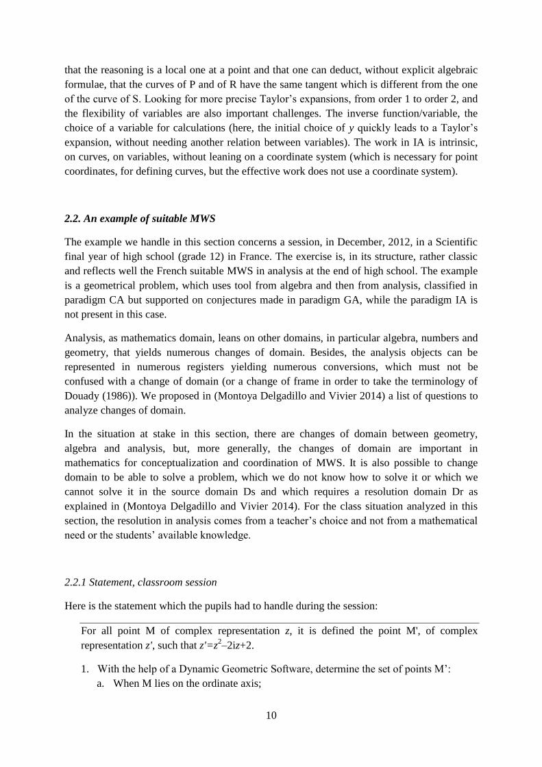
that the reasoning is a local one at a point and that one can deduct, without explicit algebraic

formulae, that the curves of P and of R have the same tangent which is different from the one

of the curve of S. Looking for more precise Taylor’s expansions, from order 1 to order 2, and

the flexibility of variables are also important challenges. The inverse function/variable, the

choice of a variable for calculations (here, the initial choice of y quickly leads to a Taylor’s

expansion, without needing another relation between variables). The work in IA is intrinsic,

on curves, on variables, without leaning on a coordinate system (which is necessary for point

coordinates, for defining curves, but the effective work does not use a coordinate system).

2.2. An example of suitable MWS

The example we handle in this section concerns a session, in December, 2012, in a Scientific

final year of high school (grade 12) in France. The exercise is, in its structure, rather classic

and reflects well the French suitable MWS in analysis at the end of high school. The example

is a geometrical problem, which uses tool from algebra and then from analysis, classified in

paradigm CA but supported on conjectures made in paradigm GA, while the paradigm IA is

not present in this case.

Analysis, as mathematics domain, leans on other domains, in particular algebra, numbers and

geometry, that yields numerous changes of domain. Besides, the analysis objects can be

represented in numerous registers yielding numerous conversions, which must not be

confused with a change of domain (or a change of frame in order to take the terminology of

Douady (1986)). We proposed in (Montoya Delgadillo and Vivier 2014) a list of questions to

analyze changes of domain.

In the situation at stake in this section, there are changes of domain between geometry,

algebra and analysis, but, more generally, the changes of domain are important in

mathematics for conceptualization and coordination of MWS. It is also possible to change

domain to be able to solve a problem, which we do not know how to solve it or which we

cannot solve it in the source domain Ds and which requires a resolution domain Dr as

explained in (Montoya Delgadillo and Vivier 2014). For the class situation analyzed in this

section, the resolution in analysis comes from a teacher’s choice and not from a mathematical

need or the students’ available knowledge.

2.2.1 Statement, classroom session

Here is the statement which the pupils had to handle during the session:

For all point M of complex representation z, it is defined the point M', of complex

representation z', such that z'=z2–2iz+2.

1. With the help of a Dynamic Geometric Software, determine the set of points M’:

a. When M lies on the ordinate axis;

11

b. When M lies on the abscissa axis.

2. Find the real part and the imaginary part of z’ setting z=x+yi, with real numbers x and

y.

3. Prove the first conjecture.

4. Likewise, prove the second conjecture.

Question 1 has to be solved at home, with the Geogebra software, and files sent to the teacher

before the session. The video session is about 40 min. We produce below a quick session

chronology.

Time Statement

1’ A student goes to the board for question 1, two conjectures are written.

8’30 Teacher explains the task of questions 2 - 3.

9’25 Individual work on question 2.

14’30 A student goes to the board to solve question 2. Expressions of x’=Re(z’) and

y’=Im(z’) as a function of x and y are given.

16’00 Student returns to his seat. Teacher asks how to use the geometrical information about

M. He gives approximately 1 min to think before asking for the answer x=0.

19’25 Individual work, students have to use this information.

21’00 Teacher writes on the board what we obtain for x' and y’ when x=0.

Teacher’s questions bring to the domain change and thus the study of the function in

the y variable which gives x' by using derivatives.

24’55 Students individually study the polynomial f(y)=-y2+2y+2.

28’50 Solutions at the board by teacher supported on his students’ answers to his questions.

Derivatives, sign of the derivative, the table of variation is made.

30’30 Calculation of f (1) and discussion about the maximum (a reminder of the theorem of

existence of an optimum in an interval for a differentiable function).

32’10 Back to conjecture, calculation of limits at -∞ and +∞. How to calculate the limit at

+∞ for a polynomial is recalled.

33’20 Identification of the interval image of f, f(R)=]-∞,3] ; the conjecture is confirmed.

Identification of the geometrical locus with the coordinates of M’.

35’08 The other conjecture, same process with y=0. It is asked to express y’ as a function of

x’. Individual research.

40’00 End of session, the exercise will be finished at the following session.

2.2.2 Domain changes

The statement of the exercise is in geometry, in the register of complex numbers5. It is a

problem of geometrical locus.

5 Of course, there is a complex function but, on one hand it is not formalized as a function and, on the other

hand, the complex analysis does not exist in French secondary education institution. Hence, the interpretation of

this statement, at the end of high school, is clearly in geometry.

12

No indication of domain change is given in the statement. Thus, one can expect to stay in

geometry, with a work in a complex register and possibly with coordinates in question 2, with

an easy sliding towards the algebra.

First indications of domain changes appear in the conjectures supported by teacher’s

questions about student’s file which is reproduced in figure 4:

● Conjecture a : « when M goes along the ordinate axis, the point M’ belongs to an

interval that is -, 3 », with a doubt: 3 belongs to the set or not?

● Conjecture b : “if M(Ox), then M’ belongs to a set which looks like a parabola

oriented to the right”.

Figure 4 : Reproduction of both locus of M’ found by student;M and M’ are renamed Ma,

M’a, Mb and M’b.

For conjecture a, indications are totally implicit with the notions of interval and expected

bound which are related to continuity. Point M’ (M’a on figure 4) moving on a straight line,

there is a priori no need of changing domain for the analysis. It is not the case for conjecture b

where, by a semiotic genesis, students recognize a parabola, even speaking of second degree

polynomial. But it is not a representative curve of a function y’=f(x’) and teacher and students

agree on this point. Nevertheless, teacher indicates the possibility of considering two

functions, one for the upper part and one for the lower part. It would be simpler to consider a

function x’=f(y’) but it is not teacher’s choice. This is close to what was evoked in section 2,

in the note 4: in CA paradigm, it is more usual to work with several functions rather than to

invert variables role – the absolute of “x” and of horizontal axis for abscissas.

Afterward, there is an algebraic work which was expected because of variables z, z' and of

their real and imaginary parts among which x and y. Thus there is a preliminary work, in a

complex and then algebra registers (the change, or conversion, is quite natural, easy, with the

algebraic form). The domain change geometry → Algebra is almost transparent and is largely

made thanks to registers at stake. We do not discuss more on this for looking more in detail to

the domain change for analysis.

13

Almost 4 min are dedicated, by teacher, to this domain change. We reproduce below teacher’s

speech, from 21’45 to 24’55, which leans on students’ answers although most of their

interventions are inaudible:

Teacher: Le point M’ appartient à l’axe (Ox), est-ce qu’il va parcourir entièrement l’axe des abscisses, ça

je ne sais pas ! et comment va-t-on savoir justement ? oui ?

A student: en faisant la limite de…

Teacher: alors pas tant la limite mais effectivement on va travailler sur x’, pas tant la limite, comment ?

Jérémy ? [a student…] alors oui, ici il y a un polynôme du deuxième degré, mais x’ c’est l’abscisse.

Apparemment l’abscisse on avait vu que ça allait de moins l’infini à 3. Donc, il va falloir que l’on fasse

quoi par rapport à x’ ? y’ c’est bon ! oui ? [a student…] oui, un tableau de variation, donc ce que l’on va

faire c’est que on va étudier donc les variations, alors avec un tableau ou non peu importe, on va étudier

les variations de x’. Alors Jérémy tu disais que x’ ça correspondait à un polynôme, étudions effectivement

ce polynôme. alors on va étudier, heeee, -y2+2y+2, que fait , -y

2+2y+2 lorsque quoi ? parce que c’est

fonction de y, vous me dites que l’on va faire un tableau de variations, mais un tableau de variations c’est

sur un ensemble de définition, ici x’ est fonction de y, la question qu’il faut se poser c’est quoi alors ? [a

student…] Parce que vous me dites que l’on va faire un tableau de variations, c’est un polynôme etc, mais

d’habitude on a x, alors on va trouver un ensemble de définition, la question d’abord, c’est par rapport à y,

donc l’ensemble de définition sera par rapport à ? [a student…] à y oui, et pas par rapport à x. Maintenant

qu’est-ce que c’est que y ? non, ce n’est pas un paramètre, qu’est-ce que c’est que y ? qu’est-ce que c’est

que y par rapport au point M ? non, z=x+iy, ça c’est une abscisse, c’est la partie imaginaire mais pour le

point M, qu’est-ce que c’est que ça ? qu’est-ce que c’est que ça ? partie réelle, partie imaginaire, pour un

point ça correspond à quoi ? voilà, c’est ça, coordonnées, abscisses, bon mais justement notre point M

dans le petit a), ben il appartient à (Oy). S’il appartient à (Oy), on a vu tout à l’heure que x=0, mais y il va

aller de quel nombre à quel nombre ? qu’est-ce qu’il va parcourir comme ensemble ? R. Sur l’axe des

imaginaires, (Oy), le point M il va aller de … - infini à + inifni. Donc effectivement, vous aller étudier ce

polynôme avec y appartenant à – infini + inifni, appartenant à R. Alors comment étudie-t-on les variations

de x’ ? [a student…] dériver. Allez-y !

If there is no indication of domain change in statement, on the other hand, teacher leads a lot

to a use the domain of analysis. He takes the responsibility of dialogues, questions, students

have only to give short answers. The word “limit” was heard most probably by the teacher in

the sense of “limit of function”, but it is possible that the student just thought of the interval

bound “3”. Then, he points, with his finger, the expression of x’ and a student says that it is a

polynomial of degree 2. Finally, another student speaks about “table of variations”, classroom

discussions are now completely into analysis. Teacher goes on until the task of studying

variations by deriving that seems to achieve completely the domain change to analysis for

him. Students, as we see it, have not much responsibility in this domain change. Teacher sets

up a suitable MWS where the domain change is guided by CA paradigm. Students only have

to make the usual sub-task (since the grade 11) to find variations of a second degree

polynomial by deriving. However, it should be noted that there is still an adaptation due to the

not usual variables: x’=f(y) instead of the usual y=f(x). Moreover, a student writes f(x’)=-

y2+2y+2 then f’(x’)=-2y+2. As one can notice it, understanding of objects at stake, links

between variables, are finally not so important in the procedural work asked by teacher.

14

It should be noted that analysis is not necessary. Indeed, one has to find the maximum of a

quadratic expression which students know from the beginning of high school6 (grade 10).

Here, it is enough to factorize: –y2+2y+2 = –(y–1)

2+3.

The activated genesis are in the Sem-Dis plan with a strong support on semiotics, teacher

emphasizes his speech by pointing expressions at the blackboard with his finger.

Hence, the domain change is rather algebra→Analysis (with a short return to algebra to solve

the equation f’(y) = -2y+2=0).

Let us note finally that there is a return to initial domain, for locus expression of M’. But

teacher is troubled because it would be necessary to convert the interval found, ]-∞,3], in

geometry. He succeed, partially, in using coordinates. It would have been possible to

introduce point A of complex representation 3 to write, for example, the half-line [A,O) or

[A,u) where u is the vector of coordinates (-1,0).

2.2.3 The teacher’s suitable MWS

Teacher’s suitable MWS is, for analysis, strongly guided by CA paradigm. It is not surprising

if one looks to teaching program of high school in analysis and overall to questions asked in

diploma at the end of French high school (baccalauréat). Nevertheless IA paradigm is

missing in this session and GA paradigm is essentially used to produce conjecture, with an

instrumented work here.

We also find the missing of continuity notion, while it is to be taught (only in an intuitive

way). Nevertheless, it is central at numerous moments. The fact that f(R)=]-∞,3] for f(y)=-

y2+2y+2 comes only from the variations table. The work is automated, naturalized, in CA

paradigm.

The use of IVT neither is indicated, what would allow to justify the reciprocal: if M belongs

to the half-right [AO), the question is whether all the points of the half-line are reached or not.

This question is not took into account in analysis, with automatic methods. But, in this case, it

seems essential to ask this question for the MWS coordination since in geometry, determining

a locus brings often to ask the reciprocal inclusion.

Teacher makes three reminders on methods:

1. To justify an optimum, the derivative has to vanish by changing sign,

2. The calculation of the limit at +of a polynomial need to consider only the term of

higher degree,

3. The sign of -2y+2 which vanishes at y=1, + or – according to the sign of the

coefficient of y.

These three procedural techniques to make tasks are typical of CA paradigm.

6 An example of optimization is given for this level in (Montoya Delgadillo et Vivier, 2014), without derivation.

15

The fact of enforcing the analysis for dealing with the expressions at stake (an important

didactic variable) and not, for problem b, intending to switch variables roles to prefer studying

two functions are two arguments in favour of CA paradigm which guides the suitable MWS

of this teacher. Obviously, there are constraints due to teaching programs and to the work

asked in baccalauréat, guided by CA paradigm. Is it possible to teach in another way at the

end of French high school? Is it doomed to: consider GA paradigm only for conjecture;

consider CA paradigm as the unique paradigm for mathematical work; exclude IA paradigm?

3. Local, global and punctual points of view

A mathematical notion can often be seen in various way. For example, a straight line can be

seen in geometry as a set of points (punctual universal), as a whole of an infinite line or an

equation (global) or still by taking points on the line as in an intersection (punctual). We find

here three of the four points of view introduced by Vandebrouck (2011) for functions. it

misses nevertheless, in the example of the geometrical line, the local point of view. It seems

that it is a specific point of view of analysis, and not only of functions. For example, for real

numbers, decimal writing allows the punctual points of view, the value of a number as

0,333… or a=0,12112111211112…, and local with a control of neighborhoods as 0,12112 are

in a ball of radius 10-5

or is an approximation of a with an error less than 10-5

. But it does not

allow a global point of view as, for example, a geometrical or interval representation does.

3.1 The three points of view

We are going to develop the case of tangent because it is a mathematical object where one can

see all these points of view in different paradigms.

The punctual point of view associated to a point on the tangent (a correspondence M→TM).

This is what one can see if the derivative exists at a point (the calculation of the equation of

the tangent line to f(x0) and f’(x0) in a paradigm AC), for example, in Geogebra, when the

button "tangent" is pressed on the point of the curve in question or when it is considered the

"perpendicular to the radio" in the circle case. The essential point is that the tangent passes

through a point and there is a use of a property that encapsulates another point of view,

without being explicit. It should be noticed that this point at stake is not necessary a tangency

point.

The global point of view is the perception of the tangent as a straight line with an equation

(paradigm AC) or a graphical rectilinear drawing (paradigm AG).

The local point of view is more related to the paradigm IA, which is based on the fact that the

tangent and the curve locally merge (property of micro-straightness of Maschietto (2002),

also with clear links to the non-standard analysis), possibly with an approximation by taking

two nearby points (cf. figure 4). One can also think that they "stick" or "touch".

16

Figure 5, grade 11 student, sciences option, who draws a tangent to a curve

It is relevant to consider that to define a tangent, it is necessary to consider these three points

of views, each focusing on different aspects. Specifically, these three points of view are

elements of the MWS genesis.

For example, in a task in the graphic register, as the one we are studying, the semiotic genesis

is activated in a different way and, specifically, through: (1) the punctual point of view when

considering the point where we must determine the tangent; (2) the local point of view by the

visualization on a small portion of the curve; (3) the global point of view by the visualization

of a graphical rectilinear trace which extends infinitely (one can note that instrumental genesis

is also activated by the artifact “ruler”).

It is possible that a point of view is absent or defective, causing opposition or difficulties for

solving a given task in a specific domain. In particular, the concept "unique intersection

point" is well known (Sierpinska 1985; Vinner 1991; Castela 1995; Páez Murillo and Vivier

2013) that is related to a perception valid at least for conic sections: a tangent is a line that

has a single point of intersection with the curve. It can also be interpreted as a depreciation of

the local point of view and a preponderance of the other two points of view with a kind of

injectivity of the correspondence of M→TM from the punctual point of view. Points of view

can explain in details several situations as we shall see.

It is expected that in these cases, a domain change (Montoya Delgadillo and Vivier, 2014)

brings points of view available in the new domain, which may be linked to different

paradigms (new points of view may be weak). In our study, we specifically expect domain

changes from geometry to analysis (paradigm AC mainly for the study population).

3.2 Points of view in graphical register

The tasks are stated in the graphic register. For 12 curves (see annex 1), it is asked to draw a

tangent which passes by a point of the curve. A priori analyses for these curves can be found

in (Montoya Delgadillo and Vivier, 2015) and (Páez Murillo and Vivier, 2013), they are not

exposed here.

These 12 curves were proposed in first university year in Chile (Montoya Delgadillo and

Vivier 2015), at the end of mathematics teachers' training in France (Vivier 2013) and in a

continuous workshop for mathematics teachers in Mexico (Páez Murillo and Vivier 2013).

17

Generally, we find the same kind of answer, with different rates in particular according to the

level of study. We propose here an analysis of some answers with points of view.

The punctual point of view is clearly at stake from the beginning. Genesis activated by

students show that there is no problem with this point of view, all the drawn lines pass by the

point at stake.

Actually, the point is to coordinate local and global points of view (a crucial coordination for

analysis objects). A good coordination of both points of view leads to a drawing like in figure

6. The activated genesis shows a local point of view which allows to draw locally the line (its

direction) then the global point of view allows to extend the drawing, possibly in cutting the

curve at another point (a tangent is a straight line). The three points of view are activated most

probably alternately, in this order, with instrumented gestures, genesis being in the Sem-Ins

plan:

1. Punctual, eyes looking at the point, ruler put on the point, with or without a pen that

points the point;

2. Local, adjustment of the ruler for a local coincidence with the curve in the

neighborhood of the considered point, a local look;

3. Global, the look is “zoomed out”, global drawing of a straight line.

Figure 6 – a French student-teacher in mathematics

This kind of answers occurs also at the beginning of university in Chile: 10 students among

44 for this curve #2 and 8 among 44 for the curve #10.

These three points of view can be found in others productions, but with a deficiency of one

point of view or a lack of coordination of local and global points of view.

In figure 7a a Mexican mathematics teacher draws the tangent by activating the punctual and

local points of view, but, because of a conception “unique intersection point”, the global point

of view is adapted and tangent becomes a strict subset of a straight line. It's the same for

French students-professors (figures 7b and 7c) with the “local” word which is used here in

opposition to “global” (while in analysis it is the dialectic global-local that is fundamental).

18

Figure7 7a (Mexico) ; figure 7b (France) ; figure 7c (France)

For this kind of answers, we find 13 of 44 Chilean students of first university year for curve

#2 and 12 on 44 for curve #10 (often without explanation).

Naturally, from the “unique intersection point” conception, other adaptations are possible. It is

possible to declare that there is no tangent (18 on 44 Chilean students of first university year

for curve #2 and 14 on 44 for curve #10). In these cases, it is rather to be a problem of

coordination of local and global points of view.

One can also think that the “unique intersection point” conception influences more widely

other students who draw a straight line without activating a local point of view, only punctual

and global points of view (with often the limitation to a subset of the straight line if it cuts the

curve at another point) as in following figures where there is a deficient local point of view.

Figure8 8a, 8b, 8c Chilean students; figure 8d, Mexican teacher

These kinds of answers have not the same impact on learning of the analysis! We think that

there is here an axis to be developed for teaching to help teachers interpreting students’

answers and proposing situations to improve students’ learning.

3.3 Points of view and domain change

7 7a : « la tangente sólo en el intervalo señalado.”; 7b : « La tangente est un élément de construction locale » ;

7c : « Ici, on peut faire qu’une tangente locale car sinon la tangente coupe la courbe une autre fois. » 8 8d: “Básicamente, no estoy segura de si este punto seria el punto de tangencia de la curva aunque por

definición podría afirmarse dicha situación, asumiendo que esta es la gráfica total de la curva”.

19

An interesting phenomenon appears during a change of domain. Indeed, in previous

productions, students remain in the graphic register and it can be assumed that the work is

essentially geometrical, in the GA paradigm.

Other students, on the other hand, make a domain change by using MWS of functions to

justify their answers, often stating “there is no tangent”, but not only. Working paradigm

becomes then CA or IA.

A Chilean student affirms, for curve #10: “No tenemos una función para aplicar derivadas y

no podemos trazar una recta que intercepta solo a B” and, for #4: “en A no existe la derivada

de la función, por lo tanto no sabemos la pendiente de la recta que pasa por A”. It is close to a

French student-teacher: “n’existe pas car le point A est un point minimum local de la courbe

donc f’(A)=0 donc le coefficient directeur de la tangente est nul”. There are some positive

arguments for curve #5, a straight line, as for this Chilean student: “la recta tangente es de

pendiente 0, es decir, es la misma línea”. In Páez Murillo and Vivier (2013), mathematics

teachers give this kind of decisive argument for the existence of a tangent to the curve #5, that

is the curve represents a linear function, which is derivable…, but it appears after more than

one hour of work, first individual, then in binomial and finally collective.

For this curve #5, a Chilean student affirms that “la tangente no existe, puesto que al ser una

función lineal, tocaría a la función en todos los puntos”. There is a domain change, but there

is also a conflict between notions of tangent in CA and in GA paradigms related to the

“unique intersection point” conception.

These arguments, obtained after a domain change, are in the CA paradigm. But there is also,

lesser frequently, arguments in IA paradigm.

Student-professor, in figure 9a, has probably visualized both parts of the curve, with the same

function, with a vertical tangent, thus of infinite derivative which he writes with a right and

left limit (also done for continuity). Naturally, it is not because he writes a limit that it is

automatically in IA paradigm. But expressing the right and left derivatives, in an unusual

situation, it let think that there was a visualization of tangents at M with M on the curve

converging towards A. It is what one sees explicitly in the negative answers of a Mexican

teacher (figures 9b and 9c). This teacher uses an argument of uniqueness in IA paradigm,

without domain change.

20

Figure9 9a : Student-teacher (France) ; figure 9b and 9c teacher (Mexico)

3.4 Conclusion on the local, global and punctual points of view

Beyond the difficulty of tangent notion, what we wanted to show it is the fact that these points

of view allow to specify, by the deficiency of one of the points of view or their coordination,

students’ errors. These analyses complete the explanation with conceptions and could have

involvements in teachers training. We postulate that it is required the three points of view,

global, local and punctual, to perform the graphical task, the defect or the reduction of one of

them leads incomplete answers and often incorrect ones, causing sometimes a drawing far

away from a tangent - however, we noticed that there is no problem with punctual point of

view.

Also, we noted a quite frequent change of domain, in particular, but not exclusive, to assert a

non-existence of the tangent. The students actually just lean on their knowledge on tangents

that is related or connected to the differentiable functions that yields uniqueness of a tangent

at a point of a curve (cf. figures 9b and 9c). The work with differentiability hides, for

tangents, the local point of view in the source domain, namely, geometry. Indeed, in AC

paradigm, there is no need for a local point of view in the MWS of functions.

4. Discussions: the perspective notion

Considering the local, global and punctual points of view of section 3 that come from the

works of Vandebrouck (2011) on functions, we observe that: the mathematical objects are the

same, they are seen through various aspects in different paradigms. We try here to widen the

concepts at stake. We call perspective to these different aspects or manners of considering

mathematical objects which can exist through different paradigms and which direct and

influence the mathematical work. Every perspective is made of several points of view, which

9 9ª :« Continuité à droite et à gauche de la tangente, et

» ; 9b: « No existe tangente sobre A porque las tangentes en las vecindades de A son

distintas » ; 9c: « No existe tangente sobre A porque aproximando las tangentes al punto A por la izquierda u la

derecha, no son las mismas. »

21

are not domain or register changes (as an integral which can be seen as an area or a

probability; in a formal register or in a graphic register).

In section 3, we pointed out three points of view linked to a localization of the view and

thought. We call it localization perspective, which consists of the local, global and punctual

points of view that we developed on the case of tangent. We can notice that this perspective is

known under the local-global dialectic often mentioned in didactics researches.

Other perspectives could be identified for analysis (and maybe more generally in the

mathematics). We find for example two points of view on curves in the section 2.1 as we

work on a tangible representation or in an intrinsic way. These two points of view, not

characteristics of the analysis, appear in both paradigms CA and IA. We could also think,

from Robert's works (Robert, 1982), of a convergence perspective with static-formal and

dynamic points of view.

Another perspective that could be called structural seems interesting to us because it is also

linked to a fundamental dialectic in analysis. In analysis, the construction of objects often uses

the discrete-continuous dialectic as, for example, the exponential whether a construction by

Euler’s method, by a geometric sequences approach (see also (Magnin and Rogalski 2011),

for a discrete approach in a physical context) or integrals by Riemann’s sums. There is a

discrete work for building continuous objects with, possibly, a first discretization stage. This

way continuous → discrete → continuous, is currently used in numerical analysis (as for the

resolution of PDE or ODE). But it also appears in an elementary work as in the following: to

make a value table for a function to place points (discrete) in a coordinate system to obtain a

representative curve (joining points continuously).

5. Conclusion

We highlight in this article the importance in mathematics, and more specifically in analysis,

of changes, whatever their nature (see (Oktaç and Vivier, to appear) for the use of changes in

mathematics education literature on analysis investigation). In (Montoya Delgadillo and

Vivier 2014) we spoke about domain changes and, here, we more specifically speak about

paradigm and points of view adding the notion of paradigm, in the MWS model it is a crucial

point of the work in this domain.

Other researches have to be led in the field of analysis in order to specify the mathematical

work. It is the main objective of the ECOS-Sud C13H03 project (http://www.irem.univ-paris-

diderot.fr/~ecosetma). Researches are in progress in particular for identifying links among

domains, analysis and probability, and on specific objects as tangent and exponential with a

development of resources for the teachers training.

Finally, we think that the identification of points of view constitutes an enhancement to

analyze finely the mathematical work. For example, comparative studies have been done with

MWS model in the field of the geometry: between Chile and France (Castela et al. 2006) and

between France and Greece (Nikolantonakis and Vivier 2014). Comparative researches on the

22

domain of analysis could make a comparison of suitable MWS, identified by means of the

methodology used in (Nikolantonakis & Vivier 2014) using implicative statistics analysis,

taking into account epistemological and cognitive plans, paradigms, domain changes as well

as points of view to specify the activated or inhibited genesis.

Acknowledgments

This work is supported by the project ECOS-Sud C13H03.

References

Beke, E. (1914). Les résultats obtenus dans l'introduction du calcul différentiel et intégral

dans les classes supérieures des établissements secondaires, L’Enseignement Mathématiques,

16, Genève.

Bergé, A. (2008). The completeness property of the set of real numbers in the transition from

calculus to analysis, Educational Studies in Mathematics, 67, 217–235.

Castela, C. (1995). Apprendre avec et contre ses connaissances antérieures, Recherches en

didactique des Mathématiques, 15(1), 7-47.

Castela, C., Consigliere, L., Guzman, I., Houdement, C., Kuzniak, A. & Rauscher, J.-C.

(2006). Paradigmes géométriques et géométrie enseignée au Chili et en France, Cahier de

DIDIREM, n° spécial 6, IREM de Paris.

Di Rico, E., Lamela, C., Luna, P. & Sessa, C. (2015). Figuras dinámicas y funciones:

representaciones vinculadas en la pantalla de Geogebra, Proceedings of CIAEM XIV, 5-7 june

2015, Tuxtla Gutiérrez, Chiapas, México.

Douady, R. (1986). Jeux de cadre et dialectique outil-objet. Recherche en Didactique des

Mathématiques, 7(2), 5-31.

Dubinsky, E., Weller, K., Michael, A. Mc Donald, M. A. & Brown, A. (2005). Some

historical issues and paradoxes regarding the concept of infinity: an APOS-based analysis:

part 2. Educational Studies in Mathematics, 60, 253-266.

Ely, R. (2010). Nonstandard Student Conceptions About Infinitesimals, Journal for Research

in Mathematics Education, 41(2), 117–146.

Estrella, S., Kuzniak, A., Montoya Delgadillo, E. & Vivier, L. (2014). El trabajo matemático

en el Análisis: una aproximación A los ETM en Francia y Chile, Actes du colloque ETM4, 30

juin-04 juillet 2014, Madrid, Espagne.

Houdement C., Kuzniak A. (2006). Paradigmes géométriques et enseignement de la

géométrie. Annales de Didactique et de Sciences Cognitives, 11, 175-193.

23

Kuzniak, A. (2006). Paradigmes et espaces de travail géométriques. Éléments d’un cadre

théorique pour l’enseignement et la formation des enseignants en géométrie. Canadian

Journal of Science and Mathematics Education, 6.2, 167-188.

Kuzniak, A. (2011). L'espace de Travail Mathématique et ses genèses. Annales de didactique

et de sciences cognitives, 16, 9-24.

Kuzniak, A. (2004). Paradigmes et espaces de travail géométriques. (Note pour l’habilitation

à diriger des recherches). Paris, France : Institut de Recherche sur l'Enseignement des

Mathématiques Paris VII.

Kuzniak, A. & Richard, P. R. (2014). Spaces for Mathematical Work. Viewpoints and

perspectives, RELIME, 17(4-I), 17-28.

Maschietto, M. (2002). L’enseignement de l’analyse au lycée: les débuts du jeu global/local

dans l’environnement de calculatrices. Thèse doctorale, Université Paris VII.

Mena-Lorca, A., Mena-Lorca, J., Montoya-Delgadillo, E., Morales, A., Parraguez, M. (2015).

El obstáculo epistemológico del infinito actual: persistencia, resistencia y categorías de

análisis, Revista Latinoamericana de Investigación en Matemática Educativa, 17(1), 1- 31.

Montoya Delgadillo, E. (2014) El proceso de prueba en el espacio de trabajo geométrico:

profesores en formación inicial. Revista Enseñanza de las Ciencias. 32(3), 227-247

Montoya Delgadillo, E. & Vivier, L. (2014). Les changements de domaine dans le cadre des

Espaces de Travail Mathématique, Annales de Didactique et de Sciences Cognitives, 19, 73-

101.

Montoya Delgadillo, E. & Vivier, L. (2015). ETM de la noción de tangente en un ámbito

gráfico - Cambios de dominios y de puntos de vista, Proceedings of CIAEM XIV, 5-7 june

2015, Tuxtla Gutiérrez, Chiapas, México.

Njomgang Ngansop & Durand-Guerrier (2014). 0, 999….. = 1 an equality questioning the

relationships between truth and validity, Proceedings of Cerme 8, Antalya, Turquie.

Nikolantonakis, K. & Vivier, L. (2014). Espaces de travail géométrique personnels mis en

œuvre par des étudiants-professeurs du premier degré en France et en Grèce lors d’une

démarche de preuve, RELIME, 17(4-I), 103-120.

Oktaç, A. & Vivier, L. Conversion, change, transition… in research about analysis, Book en

hommage à Michèle Artigue, Springer. (accepted)

Páez Murillo, R. E. & Vivier, L. (2013). Evolution of teachers’ conceptions of tangent line.

Journal of Mathematical Behavior, 32, 209-229.

Rittaud, B. & Vivier, L. (2014). Different praxeologies for rational numbers in decimal

system – the 0,9 case, Proceedings of Cerme 8, Antalya, Turquie.

24

Robert, A. (1982). L’acquisition de la notion de convergence des suites numériques dans

l’enseignement supérieur. Recherches en Didactique des Mathématiques, 3(3), 307–341.

Robinson, A.: 1966. Non-standard Analysis, North Holland.

Sierpinska, A. (1985). Obstacles épistémologiques relatifs à la notion de limite, Recherche en

Didactique des Mathématiques, 6(1), 5-67.

Tall, D. O. (1980). Intuitive infinitesimals in the calculus, Poster presented at the Fourth

International Congress on Mathematical Education, Berkeley, 1980.

Tall, D. O. & Schwarzenberger, R. L. E. (1978). Conflicts in the Learning of Real Numbers

and Limits, Mathematics Teaching, 82, 44–49.

Vandebrouck, F. (2011). Perspectives et domaines de travail pour l’étude des fonctions,

Annales de Didactique et de Sciences Cognitives, 16, 149 – 185.

Vinner, S. (1991), The role of definitions in the teaching and learning of mathematics, in

Advanced Mathematical Thinking, Edited by David Tall, Mathematics Education Library,

Kluwer, Academic Publishers, 5, 65–81.

Vivier, L. (2010). Un milieu théorique pour la notion de tangente dans l’enseignement

secondaire. Annales de Didactique et de Sciences Cognitives, 15, 167-193.

Vivier, L. (2013). Without derivatives or limits: from visual and geometrical points of view to

algebraic methods for identifying tangent lines, International Journal of Mathematic

Education in Science and Technology, 44(5), 711-717.

Weller, K., Arnon, I. & Dubinsky, E. (2009). Preservice Teachers’ Understanding of the

Relation Between a Fraction or Integer and Its Decimal Expansion, Canadian Journal of

Science, Mathematics and Technology Education, 9(1), Routeledge.

25

ANNEX 1: Curves

Instructions: For the following curve, draw a tangent at the point marked when the tangent

exists or provide an explanation if it does not exist.

#1

#2

#3

#4

#5

#6

#7

#8

#9

#10

#11

#12