Mathematical Theory of Sailing

Johan Hoffman and Claes Johnson

January 13, 2009

Abstract

We show by computational solution of the incompressible Navier-Stokes equa-tions with friction force boundary conditions, that the classical inviscid circulationtheory by Kutta-Zhukovsky for lift and laminar viscous boundary layer theory byPrandtl for drag, which have dominated 20th century fluid dynamics, do not cor-rectly describe the real turbulent airflow around a sail under tacking. We show thatlift and drag essentially originate from a turbulent wake ofcounter-rotating rolls oflow-pressure streamwise vorticity generated by a certain instability mechanism ofpotential flow at rear separation. The new theory opens the possibility of ab initiocomputational prediction of characteristics of a sailing boat using les than a mil-lion meshpoints without resolving thin boundary layers, instead of the imposssiblequadrillions required according to state-of-the-art for boundary layer resolution.

1 New Theory of Sailing

As a corollary of the resolution of d’Alembert’s paradox of zero lift/drag of potentialflow [32, 37] and the related mathematical theory of flight [34, 35, 36], we outline inthis article a mathematical theory for the generation of forward drive force and sidewayheeling force from the combined action of the sail and keel ofa sailing boat undertacking against the wind, which is fundamentally differentfrom the classical theory byKutta-Zhukovsky for lift in inviscid flow and by Prandtl for drag in viscous flow. Akeel moving through water acts like a symmetric wing generating lift which balancesthe heeling from the sail. A sail in a flow of air also acts like awing with the drivecoming from a forward component of lift and the heeling from the sideway componentof lift. But there is an important difference in the action ofa sail and a keel, with thepurpose of the sail to give forward drive at the price of heeling, and the purpose of thekeel to give lift at the price of drag. A sail requires a relatively largeangle of attackα = 15 − 25 degrees to give sufficient drive to overcome the the total drag from thesail, keel and hull, while for a keel the angle of attack is smaller with α = 5 − 10.

In thegliding flight of birds and airplanes with fixed wings at subsonic speeds, thelift/drag ratio L

D with L the lift andD the drag, is typically between 10 and 20, whichmeans that a good glider can glide up to 20 meters upon loosing1 meter in altitude, orthat Charles Lindberg could cross the Atlantic in 1927 at a speed of 50 m/s in his 2000kg Spirit of St Louisat an effective engine thrust of 150 kp (withLD = 2000/150 ≈ 13)from 100 horse powers.

1

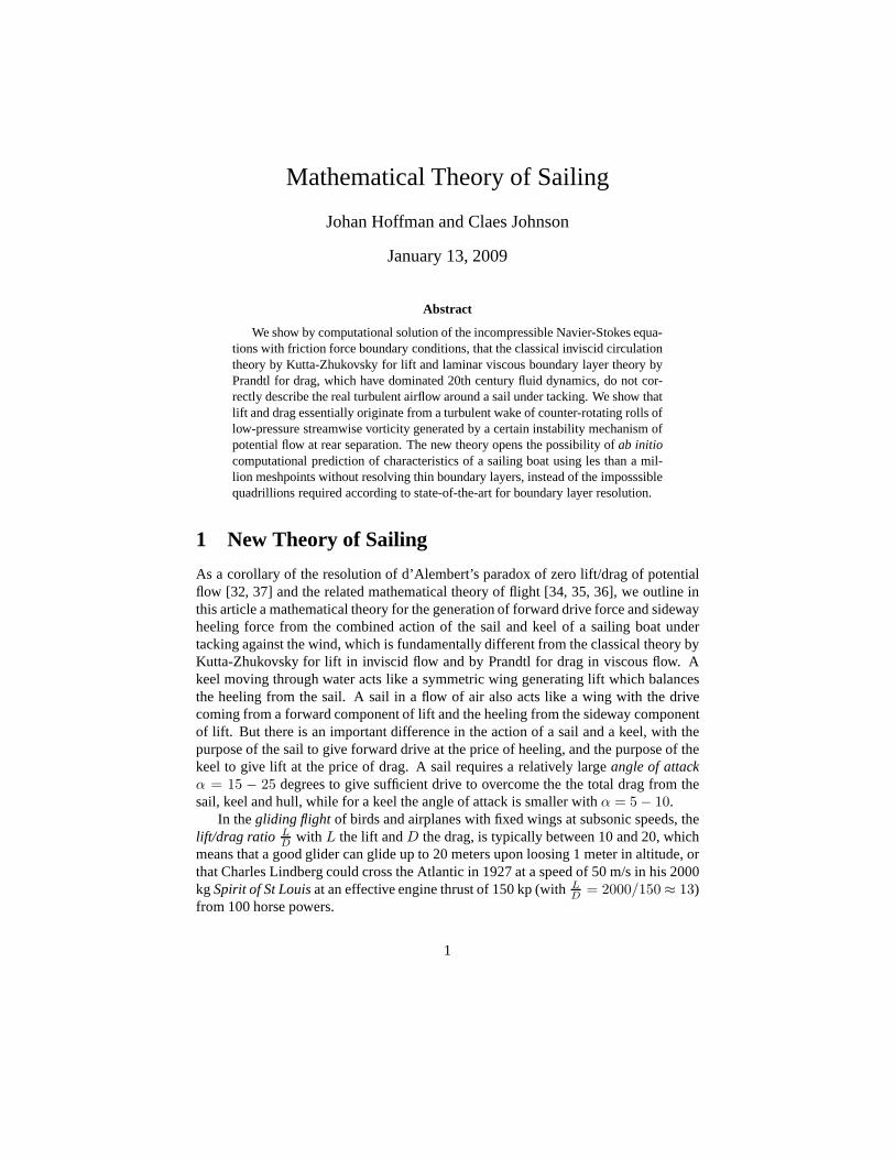
In [34] we gave a mathematical explanation based on a combination of computationand analysis of how a symmetric wing can generateL

D > 10 for 3 < α < 15, whereα is theangle of attack, and maximal lift forα = 20 with L

D ≈ 3 just before stall, asdisplayed in Fig.4. With this basis we give in this note a mathematical explanation ofthe combined action of the sail and keel of a sailing boat under tacking.

We shall find that the different shape of a sail on the windwardside, as comparedto a symmetric wing, allows a crucialLD > 6 − 10 also for the large angle of attackof α ≈ 20 required by a sail. Along the lines of [34], we will give evidence that theturbulent flow around a sail can be seen as a perturbation of zero-lift/drag potential flowresulting from a specific three-dimensional instability mechanism at separation gener-ating a turbulent wake of counter-rotating low-pressure rolls of streamwise vorticity,a mechanism which changes the pressure distribution aroundthe trailing edge so asto produce drive but also heeling. By mathematical analysisand computation we thusidentify the basic mechanism, seen as a modification of zero lift/drag potential flow,generating both drive and heeling in the real turbulent flow around a sail.

On the other hand, we give evidence that the modification by Kutta-Zhukovskyconsisting of large scale two-dimensional circulation around the section of the sail,which is the basic mechanism for lift according to classicaltheory representing state-of-the-art [23, 24], is purely fictional without counterpart in real three-dimensionalturbulent flow. Altogether we thus identify the true mechanism for drive and heelingof sail and keel, which is not captured by classical theory.

0 5 10 15 20 25 300

0.5

1

1.5

2

2.5

3

3.5

0 5 10 15 20 25 300

0.1

0.2

0.3

0.4

0.5

0.6

0.7

0.8

0.9

0 10 20 30 40 50 60 70

2

4

6

8

10

12

14

Figure 1: Lift coefficient and circulation (left), drag coefficient (middle) and lift/dragratio (right) of Naca 0012 wing as functions of angle of attack by G2 computation.

The new theory is based on the incompressible Navier-Stokesequations for slightlyviscous flow with slip (small friction force) boundary conditions as a model of a turbu-lent boundary layer coupling a solid boundary to the free stream flow through a smallskin friction force. We compute turbulent solutions of the Navier-Stokes equations us-ing a stabilized finite element method with a posteriori error control of lift and drag,referred to asGeneral Galerkinor G2, available in executable open source from [20].The stabilization in G2 acts as an automatic turbulence model, and thus offers a modelfor ab initio computational simulation of the turbulent flow around a wingwith theonly input being the geometry of the wing. Computations for asail are under way andwill be presented shortly.

We show in [31, 34] that lift and drag of a wing can be accurately predicted us-ing a couple of hundred thousand mesh points, to be compared with the impossible

2

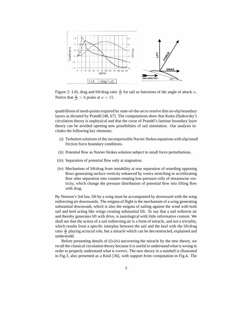
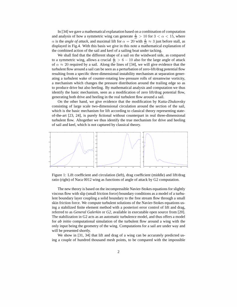
Figure 2: Lift, drag and lift/drag ratioLD for sail as functions of the angle of attackα.Notice thatL

D > 6 peaks atα = 15.

quadrillions of mesh-points required by state-of-the-artto resolve thin no-slip boundarylayers as dictated by Prandtl [48, 67]. The computations show that Kutta-Zhukovsky’scirculation theory is unphysical and that the curse of Prandtl’s laminar boundary layertheory can be avoided opening new possibilities of sail simulation. Our analysis in-cludes the following key elements:

(i) Turbulent solutions of the incompressible Navier-Stokes equations with slip/smallfriction force boundary conditions.

(ii) Potential flow as Navier-Stokes solution subject to small force perturbations.

(iii) Separation of potential flow only at stagnation.

(iv) Mechanism of lift/drag from instability at rear separation of retarding opposingflows generating surface vorticity enhanced by vortex stretching in accelleratingflow after separation into counter-rotating low-pressure rolls of streamwise vor-ticity, which change the pressure distribution of potential flow into lifting flowwith drag.

By Newton’s 3rd law, lift by a wing must be accompanied bydownwashwith the wingredirecting air downwards. The enigma of flight is the mechanism of a wing generatingsubstantial downwash, which is also the enigma of sailing against the wind with bothsail and keel acting like wings creating substantial lift. To say that a sail redirects airand thereby generates lift with drive, is tautological withlittle informative content. Weshall see that the action of a sail redirecting air is a form ofmiracle, and not a triviality,which results from a specific interplay between the sail and the keel with the lift/dragratio L

D playing acrucial role, but a miracle which can be deconstructed, explained andunderstodd.

Before presenting details of (i)-(iv) uncovering the miracle by the new theory, werecall the classical circulation theory because it is useful to understand what is wrong inorder to properly understand what is correct. The new theoryin a nutshell is illustratedin Fig.3, also presented as a Knol [36], with support from computation in Fig.4. The

3

new theory also opens to accurate simulation os sailing in open winds from the side orrear in which case the air flow around the sail is heavily turbulent. We conclude withan account of G2 for the Navier-Stokes equations.

Figure 3: Sail action in a nutshell: Windward high pressure (Hi) and leeward low pres-sure (Lo) from counter-rotating low-pressure rolls of streamwise vortices at leewardseparation (sideview left), and resulting lift L and drag D (topview middle) with angleof attackaoa indicated.

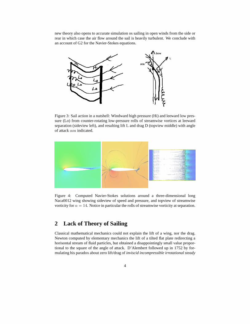
Figure 4: Computed Navier-Stokes solutions around a three-dimensional longNaca0012 wing showing sideview of speed and pressure, and topview of streamwisevorticity for α = 14. Notice in particular the rolls of streamwise vorticity at separation.

2 Lack of Theory of Sailing

Classical mathematical mechanics could not explain the lift of a wing, nor the drag.Newton computed by elementary mechanics the lift of a tiltedflat plate redirecting ahorisontal stream of fluid particles, but obtained a disappointingly small value propor-tional to the square of the angle of attack. D’Alembert followed up in 1752 by for-mulating his paradox about zero lift/drag ofinviscid incompressible irrotational steady

4

flow referred to aspotential flow, indicating that flight is mathematically impossible,or at least inexplicable. To explain flight and sailing d’Alembert’s paradox had to beresolved, and this has only been done recently, after 250 years.

It is natural to expect that today gliding flight is well understood, but surprisinglyone finds that the authority NASA [49] first dismisses three popular theories for lift asbeing incorrect (longer-path, skipping-stone,Venturi/Bernouilli), then vaguely suggestsa trivial flow-by-turning theory and ends with the empty seemingly out of reach:“Totruly understand the details of the generation of lift, one has to have a good workingknowledge of the Euler Equations”. The Plane&Pilot Magazine [52] has the samemessage. In short, state-of-the-art literature [4, 25, 64,66] presents a two-dimensionaltheory from 1903 for lift without drag at small angles of attack in inviscid potentialflow by the mathematicians Kutta and Zhukovsky, called the father of Russian aviation,and another theory for drag without lift in viscous laminar flow from 1904 by thephysicist Prandtl, called the father of modern fluid dynamics, but no theory for liftand drag inthree-dimensional slightly viscous turbulent incompressible flow such asthe flow of air around a wing of a jumbojet at the critical phaseof take-off at largeangle of attack (12 degrees) and subsonic speed (270 km/hour), as evidenced in e.g.[1, 7, 8, 10, 12, 14, 40, 43, 47].

The aero/hydromechanics of sailing is surrounded by even more confusion anddesinformation:

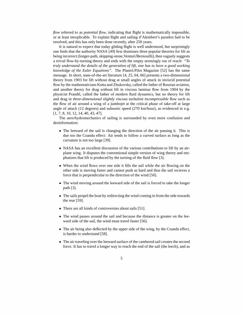
• The leeward of the sail is changing the direction of the air passing it. This isdue too the Coanda effect: Air tends to follow a curved surface as long as thecurvature is not too large [39].

• NASA has an excellent discussion of the various contributions to lift by an air-plane wing. It disputes the conventional simple version of wing theory and em-phasizes that lift is produced by the turning of the fluid flow [3].

• When the wind flows over one side it fills the sail while the air flowing on theother side is moving faster and cannot push as hard and thus the sail recieves aforce that is perpendicular to the direction of the wind [50].

• The wind moving around the leeward side of the sail is forced to take the longerpath [3].

• The sails propel the boat by redirecting the wind coming in from the side towardsthe rear [59].

• There are all kinds of controversies about sails [51].

• The wind passes around the sail and because the distance is greater on the lee-ward side of the sail, the wind must travel faster [56].

• The air being also deflected by the upper side of the wing, by the Coanda effect,is harder to understand [58].

• The air traveling over the leeward surface of the cambered sail creates the secondforce. It has to travel a longer way to reach the end of the sail(the leech), and as

5

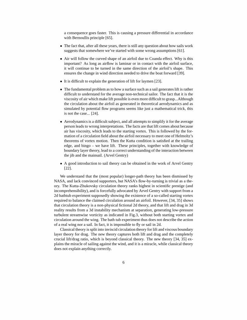
a consequence goes faster. This is causing a pressure differential in accordancewith Bernoullis principle [65].

• The fact that, after all these years, there is still any question about how sails worksuggests that somewhere we’ve started with some wrong assumptions [61].

• Air will follow the curved shape of an airfoil due to Coanda effect. Why is thisimportant? As long as airflow is laminar or in contact with theairfoil surface,it will continue to be turned in the same direction of the airfoil’s shape. Thisensures the change in wind direction needed to drive the boatforward [39].

• It is difficult to explain the generation of lift for laymen [23].

• The fundamental problem as to how a surface such as a sail generates lift is ratherdifficult to understand for the average non-technical sailor. The fact that it is theviscosity of air which make lift possible is even more difficult to grasp...Althoughthe circulation about the airfoil as generated in theoretical aerodynamics and assimulated by potential flow programs seems like just a mathematical trick, thisis not the case... [24].

• Aerodynamics is a difficult subject, and all attempts to simplify it for the averageperson leads to wrong interpretations. The facts are that lift comes about becauseair has viscosity, which leads to the starting vortex. This is followed by the for-mation of a circulation field about the airfoil necessary to meet one of Helmoltz’stheorems of vortex motion. Then the Kutta condition is satisfied at the trailingedge, and bingo – we have lift. These principles, together with knowledge ofboundary layer theory, lead to a correct understanding of the interaction betweenthe jib and the mainsail. (Arvel Gentry)

• A good introduction to sail theory can be obtained in the workof Arvel Gentry[22].

We understand that the (most popular) longer-path theory has been dismissed byNASA, and lack convinced supporters, but NASA’s flow-by-turning is trivial as a the-ory. The Kutta-Zhukovsky circulation theory ranks highestin scientific prestige (andincomprehensibility), and is forcefully advocated by Arvel Gentry with support from a2d bathtub experiment supposedly showing the existence of aso-called starting vortexrequired to balance the claimed circulation around an airfoil. However, [34, 35] showsthat circulation theory is a non-physical fictional 2d theory, and that lift and drag in 3dreality results from a 3d instability mechanism at separation, generating low-pressureturbulent streamwise vorticity as indicated in Fig.3, without both starting vortex andcirculation around the wing. The bath tub experiment thus does not describe the actionof a real wing nor a sail. In fact, it is impossible to fly or sailin 2d.

Classical theory is split into inviscid circulation theoryfor lift and viscous boundarylayer theory for drag. The new theory captures both lift and drag and the completelycrucial lift/drag ratio, which is beyond classical theory.The new theory [34, 35] ex-plains the miracle of sailing against the wind, and it is a miracle, while classical theorydoes not explain anything correctly.

6

3 Kutta-Zhukowsky and Prandtl

It took 150 years before someone dared to challenge the pessimistic mathematical pre-dictions by Newton and d’Alembert, expressed by Lord Kelvinas: “I can state flatlythat heavier than air flying machines are impossible”. In the 1890s the German en-gineer Otto Lilienthal made careful studies of the gliding flight of birds, and designedwings allowing him to make 2000 successful heavier-than-air gliding flights startingfrom a little artificial hill, before in 1896 he broke his neckfalling to the ground af-ter having stalled at 15 meters altitude. The first sustainedpowered heavier-than-airflights were performed by the two brothers Orwille and WilburWright, who on thewindy dunes of Kill Devils Hills at Kitty Hawk, North Carolina, on December 17 in1903, managed to get their 400 kg airplaneFlyer off ground into sustained flight usinga 12 horse power engine.

The undeniable presence of substantial lift now required anexplantion and to thisend Kutta and Zhukovsky augumented inviscid zero-lift potential flow by a large scaletwo-dimensionalcirculation or rotation of air around the wing section causing the ve-locity to increase above and decrease below the wing, thus generating lift proportionalto the angle of attack [66, 64], orders of magnitude larger than Newton’s prediction,but the drag was still zero. Kutta-Zhukovsky thus showed that if there is circulationthen there is lift, which by a scientific community in desperate search for a theory oflift was interpreted as an equivalence:“If the airfoil experiences lift, a circulation mustexist”, [64, 41]. State-of-the-art is described in [5] as:“The circulation theory of lift isstill alive... still evolving today, 90 years after its introduction”.

The modified potential solution is illustrated in Fig.5 indicating zones of low (L)and high (H) pressure, with the switch between high and low pressure at the trailingedge creating lift as an effect of the circulation. Kutta-Zhukovsky suggested that thecirculation around the wing section was balanced by a counter-rotating so-calledstart-ing vortexbehind the wing shown in Fig.5 (right) giving zero total circulation accordingto Kelvin’s theorem. Kutta-Zhukovsky’s formula for lift agreed reasonably well withobservations for long wings and small angles of attack, but not for short wings and largeangles of attack. We will below subject Kutta-Zhukovsky’s theory of lift to a realitytest, and we will find that it in fact is pure fiction, as much fiction as zero-lift potentialflow; the true origin of lift is not large scale two-dimensional circulation around thewing section.

In 1904 the young physicist Ludwig Prandtl took up the challenge of resolvingd’Alembert’s paradox and explaining the origin of drag in the 8 page sketchy articleMotion of Fluids with Very Little Viscosity[53] described in [55] as“one of the mostimportant fluid-dynamics papers ever written”and in [25] as“the paper will certainlyprove to be one of the most extraordinary papers of this century, and probably of manycenturies”. Prandtl suggested that the substantial drag (and lift) of a body movingthrough aslightly viscousfluid like air, possibly could arise from the presence of athin no-slip laminar viscous boundary layer, where the tangential fluid velocity rapidlychanges from zero on the boundary to the free-stream value. Prandtl argued that aflow canseparatefrom the boundary due to anadverse pressure gradientretarding theflow in a laminar boundary layer to form alow-pressure wakebehind the body creatingdrag. This is the official resolution of d’Alembert’s paradox [54, 60, 66, 16], although

7

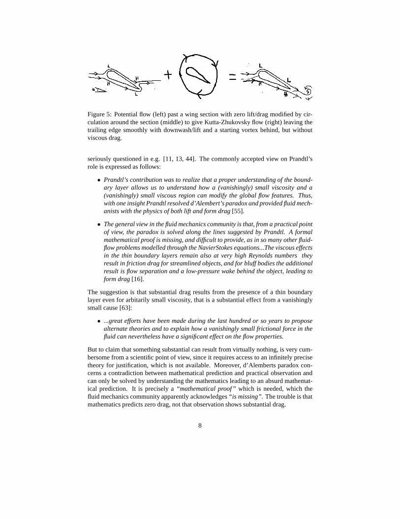
Figure 5: Potential flow (left) past a wing section with zero lift/drag modified by cir-culation around the section (middle) to give Kutta-Zhukovsky flow (right) leaving thetrailing edge smoothly with downwash/lift and a starting vortex behind, but withoutviscous drag.

seriously questioned in e.g. [11, 13, 44]. The commonly accepted view on Prandtl’srole is expressed as follows:

• Prandtl’s contribution was to realize that a proper understanding of the bound-ary layer allows us to understand how a (vanishingly) small viscosity and a(vanishingly) small viscous region can modify the global flow features. Thus,with one insight Prandtl resolved d’Alembert’s paradox andprovided fluid mech-anists with the physics of both lift and form drag[55].

• The general view in the fluid mechanics community is that, from a practical pointof view, the paradox is solved along the lines suggested by Prandtl. A formalmathematical proof is missing, and difficult to provide, as in so many other fluid-flow problems modelled through the NavierStokes equations...The viscous effectsin the thin boundary layers remain also at very high Reynoldsnumbers theyresult in friction drag for streamlined objects, and for bluff bodies the additionalresult is flow separation and a low-pressure wake behind the object, leading toform drag[16].

The suggestion is that substantial drag results from the presence of a thin boundarylayer even for arbitarily small viscosity, that is a substantial effect from a vanishinglysmall cause [63]:

• ...great efforts have been made during the last hundred or soyears to proposealternate theories and to explain how a vanishingly small frictional force in thefluid can nevertheless have a significant effect on the flow properties.

But to claim that something substantial can result from virtually nothing, is very cum-bersome from a scientific point of view, since it requires access to an infinitely precisetheory for justification, which is not available. Moreover,d’Alemberts paradox con-cerns a contradiction between mathematical prediction andpractical observation andcan only be solved by understanding the mathematics leadingto an absurd mathemat-ical prediction. It is precisely a“mathematical proof” which is needed, which thefluid mechanics community apparently acknowledges“is missing”. The trouble is thatmathematics predicts zero drag, not that observation showssubstantial drag.

8

If it is impossible to justify Prandtl’s theory, it can well be possible to disprove it:It suffices to remove the infinitely small cause (the boundarylayer) and still observethe effect (substantial drag). This is what we did in our resolution of d’Alembert’sparadox [32], but we did not remove the viscosity in the interior of the flow, whichcreates turbulent dissipation manifested in drag.

In any case, Prandtl’s resolution of d’Alembert’s paradox took fluid dynamics out ofits crisis in the early 20th century, but led computational aerodynamics into its presentparalysis described by Moin and Kim [48] as follows:

• Consider a transport airplane with a 50-meter-long fuselage and wings with achord length (the distance from the leading to the trailing edge) of about fivemeters. If the craft is cruising at 250 meters per second at analtitude of 10,000meters, about1016 grid points are required to simulate the turbulence near thesurface with reasonable detail.

But computation with1016 grid points is beyond the capacity of any thinkable com-puter, and the only way out is believed to be to designturbulence modelsfor simula-tion with millions of mesh points instead of quadrillons, but this is an open problemsince 100 years. State-of-the-art is decribed in the sequence ofAIAA Drag PredictionWork Shops[17], with however a disappointingly large spread of the 15 participatinggroups/codes reported in the blind tests of 2006. In addition, the focus is on the simplerproblem of transonic compressible flow at small angles of attack (2 degrees) of rele-vance for crusing at high speed, leaving out the more demanding problem of subsonicincompressibleflow at low speed and large angles of attack at take-off and landing,because a work shop on this topic would not draw any participants. Similar difficultiesof computing lift is reported in [41, 42]:

• Circulation control applications are difficult to compute reliably using state-of-the-art CFD methods as demonstrated by the inconsistenciesin CFD predictioncapability described in the 2004 NASA/ONR Circulation Control workshop.

4 Shortcut to Lift an Drag of a Wing

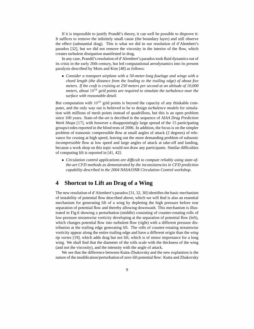
The new resolution of d’Alembert’s paradox [31, 32, 30] identifies the basic mechanismof instability of potential flow described above, which we will find is also an essentialmechanism for generating lift of a wing by depleting the highpressure before rearseparation of potential flow and thereby allowing downwash.This mechanism is illus-trated in Fig.6 showing a perturbation (middle) consistingof counter-rotating rolls oflow-pressure streamwise vorticity developing at the separation of potential flow (left),which changes potential flow into turbulent flow (right) witha different pressure dis-tribution at the trailing edge generating lift. The rolls ofcounter-rotating streamwisevorticity appear along the entire trailing edge and have a different origin than thewingtip vortex[19], which adds drag but not lift, which is of minor importance for a longwing. We shall find that the diameter of the rolls scale with the thickness of the wing(and not the viscosity), and the intensity with the angle of attack.

We see that the difference between Kutta-Zhukovsky and the new explantion is thenature of the modification/perturbationof zero-lift potential flow: Kutta and Zhukovsky

9

Figure 6: Stable physical 3d turbulent flow (right) with lift/drag, generated from po-tential flow (left) by a perturbation at separation consisting of counter-rotating rolls ofstreamwise vorticity (middle), which changes the pressureat the trailing edge generat-ing downwash/lift and drag.

claim that it consists of a global large scale two-dimensional circulation around thewing section, that istransversal vorticityorthogonal to the wing section combined witha transversal starting vortex, while we find that it is a three-dimensional local turbulentphenomenon of counter-rotating rolls of streamwise vorticity at separation, withoutstarting vortex. Kutta-Zhukovsky thus claim that lift comes from global transversalvorticity without drag, while we give evidence that insteadlift is generated by localturbulent streamwise vorticity with drag.

We observe that the real turbulent flow shares the crucial property of potential flowof adhering to the upper surface beyond the crest and thus creating downwash, becausethe real flow is similar to potential flow before separation, and because potential flowcan only separate at a point of stagnation with opposing flowsmeeting in the rear, aswe will prove below.

On the other hand, a flow with a viscous no-slip boundary layerwill (correctly ac-cording to Prandtl) separate on the crest, because in a viscous boundary layer the pres-sure gradient normal to the boundary vanishes and thus cannot contribute the normalacceleration required to keep fluid particles following thecurvature of the boundaryafter the crest, as shown in [33]. It is thus the slip boundarycondition modeling aturbulent boundary layer in slightly viscous flow, which forces the flow to suck to theupper surface and create downwash. This is a feature of incompressible irrotationalslighty viscous flow with slip, thus in particular of potential flow, and is not an effectof viscosity or molecular attractive forces as often suggested under the name of theCoanda effect. This explains why gliding flight is possible for airplanes and largerbirds, because the boundary layer is turbulent and acts likeslip preventing early sep-aration, but not for insects because the boundary layer is laminar and acts like no-slipallowing early separation.

4.1 Mechanisms of Lift and Drag

We have given evidence that the basic mechanism for the generation of lift of a wingconsists of counter-rotating rolls of low-pressure streamwise vorticity generated byinstability at separation, which reduce the high pressure on top of the wing before thetrailing edge of potential flow and thus allow downwash, but which also generate drag.At a closer examination of the quantitative distributions of lift and drag forces around

10

the wing, we discover large lift at the expense of small drag resulting from leading edgesuction, which answers the opening question of of how a wing can generate a lift/dragratio larger than 10.

The secret of flight is in concise form uncovered in Fig. 1 showing G2 computedlift and and drag coefficients of a Naca 0012 3d wing as functions of the angle of attackα, as well as the circulation around the wing. We see that the lift and drag increaseroughly linearly up to 15 degrees, with aLD > 10 for α > 3 degrees, and that lift peaksat stall atα = 20 after a quick increase of drag and flow separation at the leading edge.

We see that the circulation remains small forα less than 10 degrees without con-nection to lift, and conclude that the theory of lift of by Kutta-Zhukovsky is fictionalwithout physical correspondence: There is lift but no circulation. Lift does not origi-nate from circulation.

Inspecting Figs. 7-9 showing velocity, pressure, vorticity, and lift and drag distri-butions over the upper and lower surfaces of the wing (allowing also pitching momentto be computed), we can now, with experience from the above preparatory analysis,identify the basic mechanisms for the generation of lift anddrag in incompressiblehigh Reynolds number flow around a wing at different angles ofattackα: We find tworegimes before stall atα = 20 with different, more or less linear growth inα of bothlift and drag, a main phase0 ≤ α < 15 with the slope of the lift (coefficient) curveequal to0.09 and of the drag curve equal to0.08 with L/D ≈ 14, and a final phase15 ≤ α < 20 with increased slope of both lift and drag. The main phase canbe dividedinto an initial phase0 ≤ α < 4 − 6 and an intermediate phase4 − 6 ≤ α < 15, withsomewhat smaller slope of drag in the initial phase. We now present details of thisgeneral picture.

4.2 Phase 1: 0 ≤ α ≤ 4 − 6

At zero angle of attack with zero lift there is high pressure at the leading edge andequal low pressures on the upper and lower crests of the wing because the flow is essen-tially potential and thus satisfies Bernouilli’s law of high/low pressure where velocityis low/high. The drag is about 0.01 and results from rolls of low-pressure streamwisevorticity attaching to the trailing edge. Asα increases the low pressure below getsdepleted as the incoming flow becomes parallel to the lower surface at the trailing edgefor α = 6, while the low pressure above intenisfies and moves towards the leadingedge. The streamwise vortices at the trailing edge essentially stay constant in strengthbut gradually shift attachement towards the upper surface.The high pressure at theleading edge moves somewhat down, but contributes little tolift. Drag increases onlyslowly because of negative drag at the leading edge.

4.3 Phase 2: 4 − 6 ≤ α ≤ 15

The low pressure on top of the leading edge intensifies to create a normal gradient pre-venting separation, and thus creates lift by suction peaking on top of the leading edge.The slip boundary condition prevents separation and downwash is created with the helpof the low-pressure wake of streamwise vorticity at rear separation. The high pressure

11

at the leading edge moves further down and the pressure belowincreases slowly, con-tributing to the main lift coming from suction above. The netdrag from the uppersurface is close to zero because of the negative drag at the leading edge, known asleading edge suction, while the drag from the lower surface increases (linearly)withthe angle of the incoming flow, with somewhat increased but still small drag slope.This explains why the line to a flying kite can be almost vertical even in strong wind,and that a thick wing can have less drag than a thin.

4.4 Phase 3: 15 ≤ α ≤ 20

This is the phase creating maximal lift just before stall in which the wing partly acts as abluff body with a turbulent low-pressure wake attaching at the rear upper surface, whichcontributes extra drag and lift, doubling the slope of the lift curve to give maximal lift≈ 2.5 atα = 20 with rapid loss of lift after stall.

4.5 Lift and Drag Distribution Curves

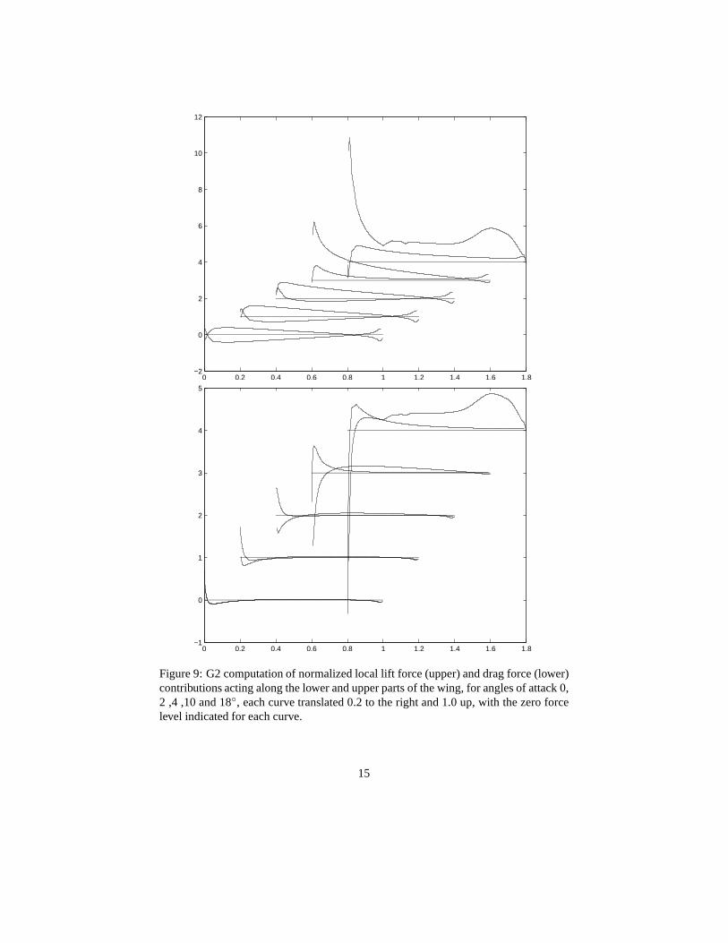
The distributions of lift and drag forces over the wing resulting from projecting thepressure acting perpendicular to the wing surface onto relevant directions, are plottedin Fig.9. The total lift and drag results from integrating these distributions around thewing. In potential flow computations (with circulation according to Kutta-Zhukovsky),only the pressure distribution orcp-distribution is considered to carry releveant infor-mation, because a potential solution by construction has zero drag. In the perspectiveof Kutta-Zhukovsky, it is thus remarkable that the projected cp-curves carry correctinformation for both lift and drag.

The lift generation in Phase 1 and 3 can rather easily be envisioned, while both thelift and drag in Phase 2 results from a (fortunate) intricateinterplay of stability andinstability of potential flow: The main lift comes from uppersurface suction arisingfrom a turbulent boundary layer with small skin friction combined with rear separationinstability generating low-pressure streamwise vorticity, while the drag is kept smallby negative drag from the leading edge. We conclude that preventing transition toturbulence at the leading edge can lead to both decreased lift and increased drag.

4.6 Comparing Computation with Experiment

Comparing G2 computations with about 150 000 mesh points with experiments [26,46], we find good agreement with the main difference that the boost of the lift co-efficient in phase 3 is lacking in experiments. This is probably an effect of smallerReynolds numbers in experiments, with a separation bubble forming on the leadingedge reducing lift at high angles of attack. The oil-film pictures in [26] show surfacevorticity generating streamwise vorticity at separation as observed also in [30, 33].

A jumbojet can only be tested in a wind tunnel as a smaller scale model, and upscal-ing test results is cumbersome because boundary layers do not scale. This means thatcomputations can be closer to reality than wind tunnel experiments. Of particular im-portance is the maximal lift coefficient, which cannot be predicted by Kutta-Zhukovsky

12

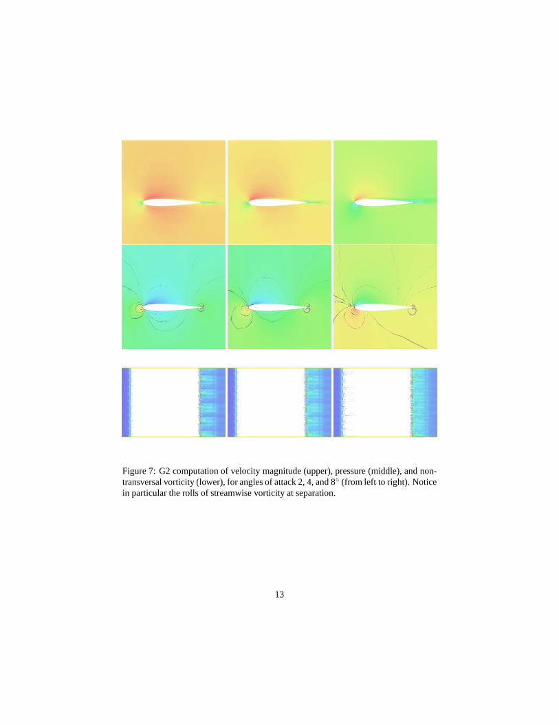
Figure 7: G2 computation of velocity magnitude (upper), pressure (middle), and non-transversal vorticity (lower), for angles of attack 2, 4, and 8 (from left to right). Noticein particular the rolls of streamwise vorticity at separation.

13

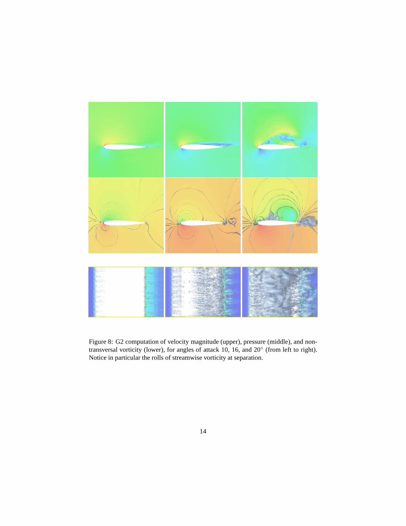
Figure 8: G2 computation of velocity magnitude (upper), pressure (middle), and non-transversal vorticity (lower), for angles of attack 10, 16,and 20 (from left to right).Notice in particular the rolls of streamwise vorticity at separation.

14

0 0.2 0.4 0.6 0.8 1 1.2 1.4 1.6 1.8−2

0

2

4

6

8

10

12

0 0.2 0.4 0.6 0.8 1 1.2 1.4 1.6 1.8−1

0

1

2

3

4

5

Figure 9: G2 computation of normalized local lift force (upper) and drag force (lower)contributions acting along the lower and upper parts of the wing, for angles of attack 0,2 ,4 ,10 and 18, each curve translated 0.2 to the right and 1.0 up, with the zero forcelevel indicated for each curve.

15

nor in model experiments, which for Boeing 737 is reported tobe 2.73 in landing incorrespondence with the computation. In take-off the maximal lift is reported to be1.75, reflected by the rapidly increasing drag beyondα = 16 in computation.

5 Shortcut to New Theory of Sailing

We now explain how the sail and keel of a sailing boat togetherpull the boat forwardin tacking at 35-45 degrees against the wind.

5.1 Key Fact 1: Sail and keel act like wings

Both the sail and keel act like wings generating lift and drag, but the action, geometricalshape and angle of attackaoa of the sail and the keel are somewhat different. Theeffectiveaoa of a sail in tacking is 15-25 degrees and that of a keel 5-10 degrees. Theaoa of the keel is also referred to as theleeway, the difference between the directionthe boat is pointed and the actual direction of travel.

5.2 Key Fact 2: Sail gives forward pull/drive at the price of heeling

The boat is pulled forward by the sail, assumingaoa = 15 with the boom inclined5degrees to the direction of the boat, by the forward drive componentsin(20)L ≈ 0.3Lof the lift L counted perpendicular to the effective wind direction, which is the usualfor a wing. There is also a side (heeling) forcecos(20)L from the sail, which tilts theboat and needs to be balanced by lift from the keel. A sail has less lift than a symmetricwing because the strong concentration of lift at the upper rounded leading edge of thewing, is missing for the sail.

The action of a sail is thus different from that of a wing: A sail gives forward pullat the price of heeling (lift), while a wing gives lift at the price of drag (backward pull).

5.3 Key Fact 3: L

Dof sail > 6 − 10

The drive from liftL is reduced by a component of the dragD counted parallel tothe effective wind direction, with similar contributions from the leeward and windwardside of the sail because the shape is the same. This makes an important difference witha symmetric wing for which the backward pull/drag is larger from the windward sidebecause of the high pressure at the lower leading edge of the wing, as displayed inFig.9.

The net result is a lift/drag ratioLD > 6−10 ataoa = 15−20 for a sail, as indicatedby Fig.2 showing thatLD for a sail peaks ataoa = 15, which reduces the drive to0.2L,Compare with Fig.1 showing thatLD ≈ 3 for a wing ataoa = 20, which would reducethe forward pull/drive to0.1L, which is too small according to:

16

5.4 Key Fact 4: Keel balances heeling at the price of drag

The heeling force from the sail is balanced by lift from the the keel in the oppositedirection. Assuming the lift/drag ratio for the keel is 10 ataoa = 5 − 10, the forwarddrive is then reduced to(0.2−0.1)L = 0.1L, which is used to overcome the drag fromthe hull minus the keel.

Note that with anLD < 3 for the sail, the net forward drive would disappear. Replac-

ing the sail by a wing thus does not seem to be a good idea, because anaoa > 15 is re-quired to get sufficient drive. But a keel like a wing works fine, because anaoa = 5−10is sufficient.

5.5 Key Fact 5: Sail area vs keel area

Assuming that the effective speed relative the air of a sail is 10 m/s ataoa = 15 andthe speed of the keel/boat through the water is 3 m/s ataoa = 5, we find (using that thedensity of water is about 800 times that of air) that the sail area can be up to25 timesthe keel area. In practice, the ratio is typically7 − 9 with a traditional full-keel and10-15 with a modern fin-keel.

5.6 Summary

The shape of a sail is different from that of a wing which givessmaller drag from thewindward side and thus improved drive, while the keel has theshape of a symmetricwing and acts like a wing. A sail withaoa = 15 − 20 gives strong drive at strongheeling with contribution also from the rear part of the sail, like for a wing just beforestall, while the drag is smaller than for a wing.

The LD curve for a sail is different from that of wing: ataoa = 15−20 L

D > 6−10

for a sail, while LD < 3 − 4 for a wing. On the other hand, a keel withaoa = 5 − 10

has LD > 6 − 10. A sail ataoa = 15 − 20 thus gives strong drive at strong heeling

and small drag, which together with a keel ataoa = 5 − 10 with strong lift and smalldrag, makes an efficient combination. This explains why modern designs combine adeep narrow keel acting efficiently for smallaoa, with a broader sail acting efficientlyat a largeraoa.

Using a symmetric wing as a sail would be inefficient, since the lift/drag ratio ispoor at maximal lift ataoa = 15 − 20. On the other hand, using a sail as a wing canonly be efficient at a large angle of attack, and thus is not suitable for cruising at higherspeed and smaller aoa.

6 Navier-Stokes with Force Boundary Conditions

The Navier-Stokes equations for an incompressible fluid of unit density withsmallviscosityν > 0 andsmall skin frictionβ ≥ 0 filling a volumeΩ in R

3 surrounding asolid body with boundaryΓ over a time intervalI = [0, T ], read as follows: Find the

17

velocityu = (u1, u2, u3) and pressurep depending on(x, t) ∈ Ω ∪ Γ × I, such that

u+ (u · ∇)u+ ∇p−∇ · σ = f in Ω × I,∇ · u = 0 in Ω × I,un = g onΓ × I,σs = βus onΓ × I,

u(·, 0) = u0 in Ω,

(1)

whereun is the fluid velocity normal toΓ, us is the tangential velocity,σ = 2νǫ(u) isthe viscous (shear) stress withǫ(u) the usual velocity strain,σs is the tangential stress,f is a given volume force,g is a given inflow/outflow velocity withg = 0 on a non-penetrable boundary, andu0 is a given initial condition. We notice the skin frictionboundary condition coupling the tangential stressσs to the tangential velocityus withthe friction coefficientβ with β = 0 for slip, andβ >> 1 for no-slip. We note thatβ isrelated to the standardskin friction coeffieientcf = 2τ

U2 with τ the tangential stress perunit area, by the relationβ = U

2 cf . In particular,β tends to zero withcf (if U staysbounded).

Concerning the size of the viscosity, we recall that for air thekinematic viscosity(normalized to unit density) is about10−5 (and for water about10−6). Normalizingalso with respect to velocity and length scale, the viscosity is represented by the inverseof the Reynolds number, which in subsonic flight ranges from105 for medium-sizebirds over107 for a smaller airplane up to109 for a jumbojet, for a sail and keel106−7.We are thus considering normalized viscosities in the rangefrom 10−5 to 10−9 to becompared with density, velocity and length scale of unit size. We understand that10−5

is smallcompared to 1, and that10−9 compared to 1 isvery small.Massive evidence indicates that the incompressible Navier-Stokes equations consti-

tute an accurate mathematical model of slightly viscous flowin subsonic aerodynamics.We will show that turbulent solutions can be computed on a laptop for simple geome-tries and on a cluster for complex geometries, with correct mean-value outputs suchas lift, drag and twisting moment of a wing or entire airplane, without resolving thinboundary layers and without resort to turbulence models. This is made possible byusing skin friction force boundary conditions for tangential stresses instead of no-slipboundary conditions for tangential velocities, and because the skin friction is smallfrom a turbulent boundary layer of a fluid with very small viscosity, and because it isnot necessary to resolve the turbulent features in the interior of the flow to physicalscales.

Prandtl insisted on using a no-slip velocity boundary condition with us = 0 on Γ,because his resolution of d’Alembert’s paradox hinged on discriminating potential flowby this condition. On the oher hand, with the new resolution of d’Alembert’s paradox,relying instead on instability of potential flow, we are freeto choose instead a frictionforce boundary condition, if data is available. Now, experiments show [60, 15] thatthe skin friction coefficient decreases with increasing Reynolds numberRe ascf ≈0.07 ∼ Re−0.2, so thatcf ≈ 0.0005 for Re = 1010 andcf ≈ 0.007 for Re = 105.Accordingly we model a turbulent boundary layer by frictionboundary condition witha friction parameterβ ≈ 0.03URe−0.2. For very large Reynolds numbers, we caneffectively useβ = 0 in G2 computation corresponding to slip boundary conditions.

18

We have initiated benchmark computations for tabulating values ofβ (or σs) fordifferent values ofRe by solving the Navier-Stokes equations with no-slip for simplegeometries such as a flat plate, and more generally for different values ofν, U andlength scale, since the dependence seems to be more complex than simply through theReynolds number. Early results are reported in [31] withσs ≈ 0.005 for ν ≈ 10−4 andU = 1, with corresponding velocity strain in the boundary layer104σs ≈ 50 indicatingthat the smallest radius of curvature without separation inthis case could be expectedto be about0.02 [33].

7 Potential Flow

Potential flow(u, p) with velocity u = ∇ϕ, whereϕ is harmonic inΩ and satisfiesa homogeneous Neumann condition onΓ and suitable conditions at infinity, can beseen as a solution of the Navier-Stokes equations for slightly viscous flow with slipboundary condition, subject to

• perturbation of the volume forcef = 0 in the form ofσ = ∇ · (2νǫ(u)),

• perturbation of zero friction in the form ofσs = 2νǫ(u)s,

with both perturbations being small becauseν is small and a potential flow velocityuis smooth. Potential flow can thus be seen as a solution of the Navier-Stokes equationswith small force perturbations tending to zero with the viscosity. We can thus expressd’Alembert’s paradox as the zero lift/drag of a Navier-Stokes solution in the form of apotential solution, and resolve the paradox by realizing that potential flow is unstableand thus cannot be observed as a physical flow.

Potential flow is like an inverted pendulum, which cannot be observed in reality be-cause it is unstable and under infinitesimal perturbations turns into a swinging motion.A stationary inverted pendulum is a fictious mathematical solution without physicalcorrespondence because it is unstable. You can only observephenomena which insome sense are stable, and an inverted pendelum or potentialflow is not stable in anysense.

Potential flow has the following crucial property which partly will be inherited byreal turbulent flow, and which explains why a flow over a wing subject to small skinfriction can avoid separating at the crest and thus generatedownwash, unlike viscousflow with no-slip, which separates at the crest without downwash. We will concludethat gliding flight is possible only in slightly viscous incompressible flow. For simplic-ity we consider two-dimensional potential flow around a cylindrical body such as longwing (or cylinder).

Theorem. Letϕ be harmonic in the domainΩ in the plane and satisfy a homogeneousNeumann condition on the smooth boundaryΓ of Ω. Then the streamlines of the cor-responding velocityu = ∇ϕ can only separate fromΓ at a point of stagnation withu = ∇ϕ = 0.Proof. Letψ be a harmonic conjugate toϕ with the pair(ϕ, ψ) satisfying the Cauchy-Riemann equations (locally) inΩ. Then the level lines ofψ are the streamlines ofϕ

19

and vice versa. This means that as long as∇ϕ 6= 0, the boundary curveΓ will be astreamline ofu and thus fluid particles cannot separate fromΓ in bounded time.

8 Exponential Instability

Subtracting the NS equations withβ = 0 for two solutions(u, p, σ) and(u, p, σ) withcorresponding (slightly) different data, we obtain the following linearized equation forthe difference(v, q, τ) ≡ (u− u, p− p, σ − σ) with :

v + (u · ∇)v + (v · ∇)u + ∇q −∇ · τ = f − f in Ω × I,∇ · v = 0 in Ω × I,v · n = g − g onΓ × I,τs = 0 onΓ × I,

v(·, 0) = u0 − u0 in Ω,

(2)

Formally, withu andu given, this is a linear convection-reaction-diffusion problem for(v, q, τ) with the reaction term given by the3 × 3 matrix∇u being the main term ofconcern for stability. By the incompressiblity, the trace of ∇u is zero, which showsthat in general∇u has eigenvalues with real value of both signs, of the size of|∇u|(with | · | som matrix norm), thus with at least one exponentially unstable eigenvalue.

Accordingly, we expect local exponential perturbation growth of sizeexp(|∇u|t)of a solution(u, p, σ), in particular we expect a potential solution to be illposed. Thisis seen in G2 solutions with slip initiated as potential flow,which subject to residualperturbations of mesh sizeh, in log(1/h) time develop into turbulent solutions. Wegive computational evidence that these turbulent solutions are wellposed, which we ra-tionalize by cancellation effects in the linearized problem, which has rapidly oscillatingcoefficients when linearized at a turbulent solution.

Formally applying the curl operator∇× to the momentum equation of (1), withν = β = 0 for simplicity, we obtain thevorticity equation

ω + (u · ∇)ω − (ω · ∇)u = ∇× f in Ω, (3)

which is a convection-reaction equation in the vorticityω = ∇ × u with coefficientsdepending onu, of the same form as the linearized equation (2), with similar prop-erties of exponential perturbation growthexp(|∇u|t) referred to asvortex stretching.Kelvin’s theorem formally follows from this equation assuming the initial vorticity iszero and∇× f = 0 (andg = 0), but exponential perturbation growth makes this con-clusion physically incorrect: We will see below that large vorticity can develop fromirrotational potential flow even with slip boundary conditions.

9 Energy Estimate with Turbulent Dissipation

The standardenergy estimatefor (1) is obtained by multiplying the momentum equa-tion

u+ (u · ∇)u+ ∇p−∇ · σ − f = 0,

20

with u and integrating in space and time, to get in the casef = 0 andg = 0,

∫ t

0

∫Ω

Rν(u, p) · u dxdt = Dν(u; t) +Bβ(u; t) (4)

whereRν(u, p) = u+ (u · ∇)u + ∇p

is theEuler residualfor a given solution(u, p) with ν > 0,

Dν(u; t) =

∫ t

0

∫Ω

ν|ǫ(u(t, x))|2dxdt

is theinternal turbulent viscous dissipation, and

Bβ(u; t) =

∫ t

0

∫Γ

β|us(t, x)|2dxdt

is theboundary turbulent viscous dissipation, from which follows by standard manip-ulations of the left hand side of (4),

Kν(u; t) +Dν(u; t) +Bβ(u; t) = K(u0), t > 0, (5)

where

Kν(u; t) =1

2

∫Ω

|u(t, x)|2dx.

This estimate shows a balance of thekinetic energyK(u; t) and theturbulent viscousdissipationDν(u; t) + Bβ(u; t), with any loss in kinetic energy appearing as viscousdissipation, and vice versa. In particular,

Dν(u; t) +Bβ(u; t) ≤ K(0),

and thus the viscous dissipation is bounded (iff = 0 andg = 0).Turbulent solutionsof (1) are characterized bysubstantial internal turbulent dissi-

pation, that is (fort bounded away from zero),

D(t) ≡ limν→0

D(uν ; t) >> 0, (6)

which is Kolmogorov’s conjecture[21]. On the other hand, the boundary dissipationdecreases with decreasing friction

limν→0

Bβ(u; t) = 0, (7)

sinceβ ∼ ν0.2 tends to zero with the viscosityν and the tangential velocityus ap-proaches the (bounded) free-stream velocity, which is not in accordance with Prandtl’sconjecture that substantial drag and turbulent dissipation originates from the boundarylayer. Kolmogorov’s conjecture (6) is consistent with

‖∇u‖0 ∼ 1√ν, ‖Rν(u, p)‖0 ∼ 1√

ν, (8)

21

where‖ · ‖0 denotes theL2(Q)-norm withQ = Ω × I. On the other hand, it followsby standard arguments from (5) that

‖Rν(u, p)‖−1 ≤√ν, (9)

where‖ · ‖−1 is the norm inL2(I;H−1(Ω)). Kolmogorov thus conjectures that the

Euler residualRν(u, p) for smallν is strongly (inL2) large, while being small weakly(in H−1).

Altogether, we understand that the resolution of d’Alembert’s paradox of explain-ing substantial drag from vanishing viscosity, consists ofrealizing that the internalturbulent dissipationD can be positive under vanishing viscosity, while the boundarydissipationB will vanish. In contradiction to Prandtl, we conclude that drag does notresult from boundary layer effects, but from internal turbulent dissipation, originatingfrom instability at separation.

10 G2 Computational Solution

We show in [31, 30, 32] that the Navier-Stokes equations (1) can be solved by G2producing turbulent solutions characterized by substantial turbulent dissipation fromthe least squares stabilization acting as an automatic turbulence model, reflecting thatthe Euler residual cannot be made small in turbulent regions. G2 has a posteriori errorcontrol based on duality and shows output uniqueness in mean-values such as lift anddrag [31, 28, 29]

We find that G2 with slip is capable of modeling slightly viscous turbulent flowwith Re > 106 of relevance in many applications in aero/hydro dynamics, includingflying, sailing, boating and car racing, with hundred thousands of mesh points in sim-ple geometry and millions in complex geometry, while according to state-of-the-artquadrillions is required [48]. This is because a friction-force/slip boundary conditioncan model a turbulent blundary layer, and interior turbulence does not have to be re-solved to physical scales to capture mean-value outputs [31].

The idea of circumventing boundary layer resolution by relaxing no-slip boundaryconditions introduced in [28, 31], was used in [9] in the formof weak satisfaction ofno-slip, which however misses the main point of using a forcecondition instead of avelocity condition.

An G2 solution(U,P ) on a mesh with local mesh sizeh(x, t) according to [31],satisfies the following energy estimate (withf = 0, g = 0 andβ = 0):

K(U(t)) +Dh(U ; t) = K(u0), (10)

where

Dh(U ; t) =

∫ t

0

∫Ω

h|Rh(U,P )|2 dxdt, (11)

is an analog ofDν(u; t) with h ∼ ν, whereRh(U,P ) is the Euler residual of(U,P )We see that the G2 turbulent viscosityDh(U ; t) arises from penalization of a non-zero

22

Euler residualRh(U,P ) with the penalty directly connecting to the violation (accord-ing the theory of criminology). A turbulent solution is characterized by substantialdissipationDh(U ; t) with ‖Rh(U,P )‖0 ∼ h−1/2, and

‖Rh(U,P )‖−1 ≤√h (12)

in accordance with (8) and (9).

11 Wellposedness of Mean-Value Outputs

LetM(v) =∫

Qvψdxdt be amean-value outputof a velocityv defined by a smooth

weight-functionψ(x, t), and let(u, p) and(U,P ) be two G2-solutions on two mesheswith maximal mesh sizeh. Let (ϕ, θ) be the solution to thedual linearized problem

−ϕ− (u · ∇)ϕ+ ∇U⊤ϕ+ ∇θ = ψ in Ω × I,∇ · ϕ = 0 in Ω × I,ϕ · n = g onΓ × I,

ϕ(·, T ) = 0 in Ω,

(13)

where⊤ denotes transpose. Multiplying the first equation byu−U and integrating byparts, we obtain the following output error representation[31, ?]:

M(u) −M(U) =

∫Q

(Rh(u, p) −Rh(U,P )) · ϕdxdt (14)

where for simplicity the dissipative terms are here omitted, from which follows the aposteriori error estimate:

|M(u) −M(U)| ≤ S(‖Rh(u, p)‖−1 + ‖Rh(U,P )‖−1), (15)

where the stability factor

S = S(u, U,M) = S(u, U) = ‖ϕ‖H1(Q). (16)

In [31] we present a variety of evidence, obtained by computational solution of thedual problem, that for global mean-value outputs such as drag and lift,S << 1/

√h,

while‖R‖−1 ∼√h, allowing computation of of drag/lift with a posteriori error control

of the output within a tolerance of a few percent. In short, mean-value outputs such aslift amd drag are wellposed and thus physically meaningful.

We explain in [31] the crucial fact thatS << 1/√h, heuristically as an effect of

cancellationrapidly oscillating reaction coefficients of turbulent solutions combinedwith smooth data in the dual problem for mean-value outputs.In smooth potentialflow there is no cancellation, which explains why zero lift/drag cannot be observed inphysical flows.

As an example, we show in Fig.10 turbulent G2 flow around a car with substantialdrag in accordance with wind-tunnel experiments. We see a pattern of streamwisevorticity forming in the rear wake. We also see surface vorticity forming on the hoodtransversal to the main flow direction. We will below discover similar features in theflow of air around a wing.

23

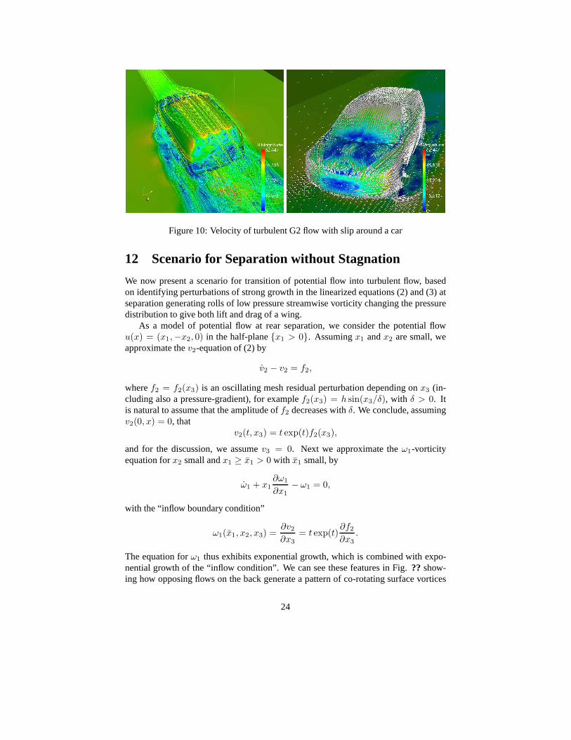
Figure 10: Velocity of turbulent G2 flow with slip around a car

12 Scenario for Separation without Stagnation

We now present a scenario for transition of potential flow into turbulent flow, basedon identifying perturbations of strong growth in the linearized equations (2) and (3) atseparation generating rolls of low pressure streamwise vorticity changing the pressuredistribution to give both lift and drag of a wing.

As a model of potential flow at rear separation, we consider the potential flowu(x) = (x1,−x2, 0) in the half-planex1 > 0. Assumingx1 andx2 are small, weapproximate thev2-equation of (2) by

v2 − v2 = f2,

wheref2 = f2(x3) is an oscillating mesh residual perturbation depending onx3 (in-cluding also a pressure-gradient), for examplef2(x3) = h sin(x3/δ), with δ > 0. Itis natural to assume that the amplitude off2 decreases withδ. We conclude, assumingv2(0, x) = 0, that

v2(t, x3) = t exp(t)f2(x3),

and for the discussion, we assumev3 = 0. Next we approximate theω1-vorticityequation forx2 small andx1 ≥ x1 > 0 with x1 small, by

ω1 + x1∂ω1

∂x1− ω1 = 0,

with the “inflow boundary condition”

ω1(x1, x2, x3) =∂v2∂x3

= t exp(t)∂f2∂x3

.

The equation forω1 thus exhibits exponential growth, which is combined with expo-nential growth of the “inflow condition”. We can see these features in Fig.?? show-ing how opposing flows on the back generate a pattern of co-rotating surface vortices

24

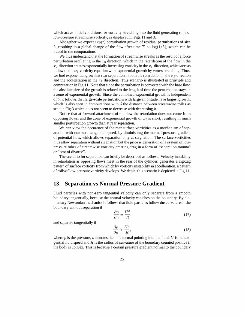
which act as initial conditions for vorticity stretching into the fluid generating rolls oflow-pressure streamwise vorticity, as displayed in Figs.11 and 3.

Altogether we expectexp(t) perturbation growth of residual perturbations of sizeh, resulting in a global change of the flow after timeT ∼ log(1/h), which can betraced in the computations.

We thus understand that the formation of streamwise streaksas the result of a forceperturbation oscillating in thex3 direction, which in the retardation of the flow in thex2-direction creates exponentially increasing vorticity inthex1-direction, which acts asinflow to theω1-vorticity equation with exponential growth by vortex stretching. Thus,we find exponential growth at rear separation in both the retardation in thex2-directionand the accelleration in thex1 direction. This scenario is illustrated in principle andcomputation in Fig.11. Note that since the perturbation is convected with the base flow,the absolute size of the growth is related to the length of time the perturbation stays ina zone of exponential growth. Since the combined exponential growth is independentof δ, it follows that large-scale perturbations with large amplitude have largest growth,which is also seen in computations withδ the distance between streamwise rollss asseen in Fig.3 which does not seem to decrease with decreasingh.

Notice that at forward attachment of the flow the retardationdoes not come fromopposing flows, and the zone of exponential growth ofω2 is short, resulting in muchsmaller perturbation growth than at rear separation.

We can view the occurence of the rear surface vorticities as amechanism of sep-aration with non-zero tangential speed, by diminishing thenormal pressure gradientof potential flow, which allows separation only at stagnation. The surface vorticitiesthus allow separation without stagnation but the price is generation of a system of low-pressure tubes of streamwise vorticity creating drag in a form of “separation trauma”or “cost of divorce”.

The scenario for separation can briefly be described as follows: Velocity instabilityin retardation as opposing flows meet in the rear of the cylinder, generates a zig-zagpattern of surface vorticity from which by vorticity instability in accelleration, a patternof rolls of low-pressure vorticity develops. We depict thisscenario is depicted in Fig.11.

13 Separation vs Normal Pressure Gradient

Fluid particles with non-zero tangential velocity can onlyseparate from a smoothboundary tangentially, because the normal velocity vanishes on the boundary. By ele-mentary Newtonian mechanics it follows that fluid particlesfollow the curvature of theboundary without separation if

∂p

∂n=U2

R(17)

and separate tangentially if∂p

∂n<U2

R, (18)

wherep is the pressure,n denotes the unit normal pointing into the fluid,U is the tan-gential fluid speed andR is the radius of curvature of the boundary counted positive ifthe body is convex. This is because a certain pressure gradient normal to the boundary

25

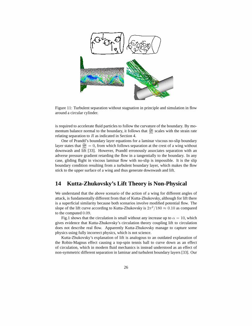
Figure 11: Turbulent separation without stagnation in principle and simulation in flowaround a circular cylinder.

is required to accelerate fluid particles to follow the curvature of the boundary. By mo-mentum balance normal to the boundary, it follows that∂p

∂n scales with the strain raterelating separation toR as indicated in Section 4.

One of Prandtl’s boundary layer equations for a laminar viscous no-slip boundarylayer states that∂p

∂n = 0, from which follows separation at the crest of a wing withoutdownwash and lift [33]. However, Prandtl erronously associates separation with anadverse pressure gradient retarding the flow in a tangentially to the boundary. In anycase, gliding flight in viscous laminar flow with no-slip is impossible. It is the slipboundary condition resulting from a turbulent boundary layer, which makes the flowstick to the upper surface of a wing and thus generate downwash and lift.

14 Kutta-Zhukovsky’s Lift Theory is Non-Physical

We understand that the above scenario of the action of a wing for different angles ofattack, is fundamentally different from that of Kutta-Zhukovsky, although for lift thereis a superficial similarity because both scenarios involve modified potential flow. Theslope of the lift curve according to Kutta-Zhukovsky is2π2/180 ≈ 0.10 as comparedto the computed0.09.

Fig.1 shows that the circulation is small without any increase up toα = 10, whichgives evidence that Kutta-Zhukovsky’s circulation theorycoupling lift to circulationdoes not describe real flow. Apparently Kutta-Zhukovsky manage to capture somephysics using fully incorrect physics, which is not science.

Kutta-Zhukovsky’s explanation of lift is analogous to an outdated explanation ofthe Robin-Magnus effect causing a top-spin tennis ball to curve down as an effectof circulation, which in modern fluid mechanics is instead understood as an effect ofnon-symmetric different separation in laminar and turbulent boundary layers [33]. Our

26

Figure 12: Separation in slightly viscous flow with slip overa smooth hill by generationof surface vorticity. Notice that the flow separates after the crest

results show that Kutta-Zhukovsky’s lift theory for a wing also needs to be replaced.

References

[1] How Airplanes Fly: A Physical Description of Lift, http://www.allstar.fiu.edu/aero/airflylvl3.htm.

[2] Bryon D. Anderson, The Physics of Sailing, Explained, Sheridan House, 2003.

[3] Bryon D. Anderson, The Physics of Sailing, EverydayScientist,http://blog.everydayscientist.com/wp-content/uploads/physics-sailing.pdf,http : //www.sciencedaily.com/videos/2007/1208− physicsofsailing.htm

[4] J. D. Anderson,A History of Aerodynamics, Cambridge Aerospace Series 8, Cam-bridge University Press, 1997.

[5] J D. Anderson, Ludwig Prandtl’s Boundary Layer,http://www.aps.org/units/dfd/resources/upload/prandtlvol58no12p4248.pdf

[6] H. Ashley, Engineering Analysis of Flight Vehicles, Addison-Wesley AerospaceSeries, Addison-Wesley, Reading, Mass., 1974, Sect 4.3.4.

[7] http://www.aviation-history.com/theory/lift.htm

[8] AVweb, http://www.avweb.com/news/airman/183261-1.html.

27

[9] Y. Bazilevs, C. Michler, V.M. Calo and T.J.R. Hughes, Turbulence without Tears:Residual-Based VMS, Weak Boundary Conditions, and Isogeometric Analysis ofWall-Bounded Flows, Preprint 2008.

[10] W. Beaty, Airfoil Lifting Force Misconception Widespread in K-6 Textbooks,Science Hobbyist, http://www.eskimo.com/ billb/wing/airfoil.htm#L1.

[11] Garret Birkhoff,Hydrodynamics: a study in logic, fact and similitude, PrincetonUniversity Press, 1950.

[12] K. Chang, Staying Aloft; What Does Keep Them Up There?, New York Times,Dec 9, 2003.

[13] S. Cowley, Laminar boundary layer theory: A 20th century paradox, Proceedingsof ICTAM 2000, eds. H. Aref and J.W. Phillips, 389-411, Kluwer (2001).

[14] G. M. Craig, Stop Abusing Bernoulli! - How Airplanes Really Fly, RegenerativePress, 1998.

[15] A. Crook, Skin friction estimation at high Reynolds numbers and Reynolds-number effects for transport aircraft, Center for Turbulence Research, 2002.

[16] D’Alembert’s paradox, en.wikipedia.org/wiki/D’Alembert’sparadox.

[17] 3rd CFD AIAA Drag Prediction Workshop, aaac.larc.nasa.gov/tfcab/cfdlarc/aiaa-dpw.

[18] O. Darrigol, World of Flow, A History of hydrodynamics from the Bernouillis toPrandtl, Oxford University Press.

[19] A. Fage and L.F. Simmons, An investigation of the air-flow pattern in the wakeof an airfoil of finite span, Rep.Memor.aero.REs.Coun.,Lond.951, 1925.

[20] The FEniCS Project, www.fenics.org.

[21] U. Frisch, Turbulence: The Legacy of A. N. Kolmogorov. Cambridge UniversityPress, 1995.

[22] fx sails, http://www.fxsails.com/recommendedreadingarticle.php.

[23] A. Gentry, A Review of Modern Sail Theory, Proc. 11th AIAA Symposium onthe Aero/Hydronautics of Sailing, 1981.

[24] A. Gentry, The Application of CFD to Sails, Proc. Symp. on Hydrodynamic Per-formance Enhancement for Marine Applications, 1988.

[25] S. Goldstein, Fluid mechanics in the first half of this century, in Annual Reviewof Fluid Mechanics, Vol 1, ed. W. R. Sears and M. Van Dyke, pp 1-28, Palo Alto,CA: Annuak Reviews Inc.

28

[26] N. Gregory and C.L. O’Reilly, Low-Speed Aerodynamic Characteristics ofNACA 0012 Aerofoil Section, including the Effects of Upper-Surface RoughnessSimulating Hoar Frost, Aeronautical Research Council Reports and Memoranda,http://aerade.cranfield.ac.uk/ara/arc/rm/3726.pdf.

[27] Heikki Hansen, Enhanced Wind Tunnel Techniques and Aerodynamic ForceModels for Yacht Sails, Ph D Thesis, University of Auckland,2006.

[28] J.Hoffman, Simulation of turbulent flow past bluff bodies on coarse meshes usingGeneral Galerkin methods: drag crisis and turbulent Euler solutions, Comp. Mech.38 pp.390-402, 2006.

[29] J. Hoffman, Simulating Drag Crisis for a Sphere using Friction Boundary Condi-tions, Proc. ECCOMAS, 2006.

[30] J. Hoffman and C. Johnson, Blowup of Euler solutions, BIT Numerical Mathe-matics, Vol 48, No 2, 285-307.

[31] J. Hoffman and C. Johnson,Computational Turbulent Incompressible Flow,Springer, 2007, www.bodysoulmath.org/books.

[32] J. Hoffman and C. Johnson, Resolution of d’Alembert’s paradox, Journal ofMathematical Fluid Mechanics, Online First, Dec 10, 2008.

[33] J. Hoffman and C. Johnson, Separation in slightly viscous flow, submitted toPhysics of Fluids.

[34] J. Hoffman and C. Johnson, Mathematical Theory of Flight, submitted to Journalof Mathematical Fluid Mechanics.

[35] Why It Is Posible to Fly, http://knol.google.com/k/claes-johnson/why-it-is-possible-to-fly/yvfu3xg7d7wt/18.

[36] Why It Is Posible to Sail, http://knol.google.com/k/claes-johnson/why-it-is-possible-to-sail/yvfu3xg7d7wt/20.

[37] http://knol.google.com/k/claes-johnson/dalemberts-paradox/yvfu3xg7d7wt/2.

[38] http://knol.google.com/k/claes-johnson/why-it-is-possible-to-fly/yvfu3xg7d7wt/18.

[39] Hoe Sails Work,http : //sail−boats.suite101.com/article.cfm/howsailswork.

[40] HowStuffWorks, http://science.howstuffworks.com/airplane7.htm.

[41] G.S. Jones, J.C. Lin, B.G. Allan, W.E. Milholen, C.L. Rumsey,R.C. Swanson,Overview of CFD Validation Experiments for Circulation Control Applications atNASA.

[42] G.S. Jones, R.D. Joslin, Proceedings of the 2004 NASA/ONR Circulation ControlWorkshop, NASA/CP-2005-213509, June 2005.

29

[43] R. Kunzig, An old, lofty theory of how airplanes fly losessome altitude, Discover,Vol. 22 No. 04, April 2001.

[44] F. W. Lanchester,Aerodynamics, 1907.

[45] Experiments in Aerodynamics, Smithsonian Contributions to Knowledge no. 801,Washinton, DC, Smithsonian Institution.

[46] W. J. McCroskey, A Critical Assessment of Wind Tunnel Results for the NACA0012 Airfoil, NASA Technical Memorandum 10001, Technical Report 87-A-5,Aeroflightdynamics Directorate, U.S. Army Aviation Research and TechnologyActivity, Ames Research Center, Moffett Field, California.

[47] http://web.mit.edu/16.00/www/aec/flight.html.

[48] P. Moin and J. Kim, Tackling Turbulence with Supercomputers, Scientific Amer-ican Magazine, 1997.

[49] http://www.grc.nasa.gov/WWW/K-12/airplane/lift1.html.

[50] The Physics of Sailing, http : //ffden −2.phys.uaf.edu/211fall2002.web.dir/joshpalmer/basic.html.

[51] The Physics of Sailing, http://www.kqed.org/quest/television/the-physics-of-sailing.

[52] http://www.planeandpilotmag.com/aircraft/specifications/diamond/2007-diamond-star-da40-xl/289.html

[53] L. Prandtl, On Motion of Fluids with Very Little, in Verhandlungen des drit-ten internationalen Mathematiker-Kongresses in Heidelberg 1904, A. Krazer, ed.,Teubner, Leipzig, Germany (1905), p. 484. English trans. inEarly Developmentsof Modern Aerodynamics, J. A. K. Ack- royd, B.P. Axcell, A.I.Ruban, eds.,Butterworth-Heinemann, Oxford, UK (2001), p. 77.

[54] L. Prandtl and O Tietjens,Applied Hydro- and Aeromechanics, 1934.

[55] http://www.imechanica.org/node/1477.

[56] QUBSailingClub, http://quis.qub.ac.uk/sailing/techinfo/techintr.htm.

[57] C. Rumsey and R. Wahls, Focussed assessment of state-of-the-art CFD capabil-ities for prediction of subsonic fixed wing aircraft aerodynamics, NASA LangleyResearch Center, NASA-TM-2008-215318.

[58] Sail Theory, http://www.sailtheory.com/index.html.

[59] Sail, Wikipedia, http://en.wikipedia.org/wiki/Sail.

[60] H. Schlichting, Boundary Layer Theory, McGraw-Hill, 1979.

[61] Sailing World Magazine, http://www.arvelgentry.com/magaz/wgaca.pdf.

30

[62] http://www.straightdope.com/columns/read/2214/how-do-airplanes-fly-really.

[63] K. Stewartson, D’Alembert’s Paradox, SIAM Review, Vol. 23, No. 3, 308-343.Jul., 1981.

[64] B. Thwaites (ed),Incompressible Aerodynamics, An Account of the Theory andObservation of the Steady Flow of Incompressible Fluid pas Aerofoils, Wings andother Bodies, Fluid Motions Memoirs, Clarendon Press, Oxford 1960, Dover 1987,p 94.

[65] Basic Sailing Theory, University of Hawaii,http://www.uhh.hawaii.edu/sailing/UHHSailingSite%20folder/UHHSailingSite/SailingTheory1.html

[66] R. von Mises, Theory of Flight, McGraw-Hill, 1945.

[67] D. You and P. Moin, Large eddy simulation of separation over an airfoil withsynthetic jet control, Center for Turbulence Research, 2006.

31